Revisiting Co-Processing for Hash Joins on the Coupled CPU-GPU Architecture

Abstract

Query co-processing on graphics processors (GPUs) has become an effective means to improve the performance of main memory databases. However, the relatively low bandwidth and high latency of the PCI-e bus are usually bottleneck issues for co-processing. Recently, coupled CPU-GPU architectures have received a lot of attention, e.g. AMD APUs with the CPU and the GPU integrated into a single chip. That opens up new opportunities for optimizing query co-processing. In this paper, we experimentally revisit hash joins, one of the most important join algorithms for main memory databases, on a coupled CPU-GPU architecture. Particularly, we study the fine-grained co-processing mechanisms on hash joins with and without partitioning. The co-processing outlines an interesting design space. We extend existing cost models to automatically guide decisions on the design space. Our experimental results on a recent AMD APU show that (1) the coupled architecture enables fine-grained co-processing and cache reuses, which are inefficient on discrete CPU-GPU architectures; (2) the cost model can automatically guide the design and tuning knobs in the design space; (3) fine-grained co-processing achieves up to 53%, 35% and 28% performance improvement over CPU-only, GPU-only and conventional CPU-GPU co-processing, respectively. We believe that the insights and implications from this study are initial yet important for further research on query co-processing on coupled CPU-GPU architectures.

1 Introduction

Query co-processing on GPUs (or Graphics Processing Units) have been an effective means to improve the performance of main memory databases(e.g., [15, 12, 17, 28, 22, 21]). Compared with CPUs, GPUs have rather high memory bandwidth and massive thread parallelism, which is ideal for data parallelism in query processing. Designed as a co-processor, the GPU is usually connected to the CPU with a PCI-e bus. So far, most research studies on GPU query co-processing have been conducted on such discrete CPU-GPU architectures. The relatively low bandwidth and high latency of the PCI-e bus are usually bottleneck issues [15, 12, 28, 21]. GPU co-processing algorithms have to be carefully designed so that the overhead of data transfer on PCI-e is minimized. Recently, hardware vendors have attempted to resolve this overhead with new architectures. We have seen integrated chips with coupled CPU-GPU architectures. The CPU and the GPU are integrated into a single chip, avoiding the costly data transfer via the PCI-e bus. For example, the AMD APU (Accelerated Processing Unit) architecture integrates the CPU and the GPU into a single chip, and Intel released their latest generation Ivy Bridge processor in late April, 2012. These new heterogeneous architectures potentially open up new optimization opportunities for GPU query co-processing. Since hash joins have been extensively studied on both CPUs and GPUs and are one of the most important join algorithms for main memory databases, this paper revisits co-processing for hash joins on the coupled CPU-GPU architecture.

Before exploring the new opportunities by the coupled architecture, let us analyze the performance issues of query co-processing on discrete architectures. A number of hash join algorithms have been developed for CPU-GPU co-processing on the discrete architecture [17, 21, 22]. The data transfer on the PCI-e bus is an inevitable overhead, although it is feasible to reduce this overhead by overlapping computation and data transfer. This data transfer leads to coarse-grained query co-processing schemes. Most studies off-load the entire join to the GPU, and the CPU is usually under-utilized during the join process. On the other hand, co-processing on the discrete architecture under-utilizes the data cache, because the CPU and the GPU have their own caches. This prohibits cache reuse among processors to reduce the memory stall, which is one of the major performance factors for hash joins [1, 27].

By integrating the CPU and the GPU into the same chip, the coupled architecture eliminates the data transfer overhead of the PCI-e bus. Existing query co-processing algorithms (e.g., [21, 22]) can immediately gain this performance improvement. However, a natural question is whether and how we can further improve the performance of co-processing on the coupled architecture. Considering the above-mentioned performance issues of co-processing on discrete architectures, we find that the two hardware features of the coupled architecture lead to significant implications on the effectiveness of co-processing.

Firstly, unlike discrete architectures where the CPU and the GPU have their own memory hierarchy, the CPU and the GPU in the coupled architecture share the same physical main memory. Furthermore, they can share some levels of the cache hierarchy (e.g., the CPU and the GPU in the AMD APU share the L2 data cache). The CPU and the GPU can communicate at the memory (or even cache) speed, and more fine-grained co-processing designs and data sharing are feasible, which are inefficient on the discrete architecture.

Secondly, due to the limited chip area, the GPU in the coupled architecture is usually less powerful than the high-end GPU in discrete architectures (see Table 1 of Section 2). The GPU in the coupled architecture usually cannot deliver a dominant performance speedup as it does in discrete architectures. Therefore, a good co-processing scheme must keep both processors busy as well as carefully assigning workloads to them for the maximized speedup.

In this paper, we revisit co-processing schemes for hash joins on such CPU-GPU coupled architectures. Specifically, we examine both hash joins with and without partitioning, and explore the design space of fine-grained co-processing on the coupled architecture. Additionally, we consider a series of design tradeoffs such as whether the hash table should be shared or separated between the two processors as well as different co-processing granularities. We extend existing cost models to predict the performance of hash joins with different co-processing schemes, and thus guide the decisions on co-processing design space.

We implement all co-processing schemes of hash joins with OpenCL on AMD APU A8 3870K. The major experimental results are summarized as follows.

First, we evaluate the co-processing schemes on the (emulated) discrete architecture in comparison with the coupled architecture, and show that (1) conventional co-processing of hash joins [17, 22] can achieve only marginal performance improvement on the coupled architecture; (2) the coupled architecture enables fine-grained co-processing and cache reuse optimizations, which are inefficient/infeasible on discrete architectures (Section 5.2).

Second, we evaluate the cost model and show that our cost model is able to effectively guide the decision on the optimizations in the design space (Section 5.3).

Third, we evaluate a number of design tradeoffs on the fine-grained co-processing, which are important for the hash join performance (Section 5.4).

Fourth, we evaluate a number of co-processing variants, and show that fine-grained co-processing achieves up to 53%, 35% and 28% performance improvement compared with CPU-only, GPU-only and conventional CPU-GPU co-processing, respectively (Section 5.5).

To the best of our knowledge, this is the first systematic study of hash join co-processing on the coupled architecture. We believe that the insights and implications from this study can shed light on further research of query co-processing on CPU-GPU coupled architectures.

Organization. The remainder of this paper is organized as follows. In Section 2, we briefly introduce background and related work. In Section 3, we revisit fine-grained CPU-GPU co-processing schemes for hash joins. The cost model is described in Section 4. We present the experimental results in Section 5 and conclude in Section 6.

2 Preliminaries and Related Work

We first introduce CPU-GPU architectures and OpenCL, and then review the related work on hash joins.

2.1 Coupled CPU-GPU Architecture

GPUs have emerged as promising hardware co-processors to speedup various applications, such as scientific computing [33] and database operations [17]. With massive thread parallelism and high memory bandwidth, GPUs are suitable for applications with massive data parallelism and high computation intensity.

One hurdle for the effectiveness of CPU-GPU co-processing is that the GPU is usually connected with the CPU with a PCI-e bus, as illustrated in Figure 1 (a). On such discrete architectures, the mismatch between the PCI-e bandwidth (e.g., 4–8 GB/sec) and CPU/GPU memory bandwidth (e.g., dozens to hundreds of GB/sec) can offset the overall performance of CPU-GPU co-processing. As a result, it is preferred to have coarse-grained co-processing to reduce the data transfer on the PCI-e bus. Moreover, as the GPU and the CPU have their own memory controllers and caches (such as L2 data cache), data accesses are in different paths.

(a) Discrete

(b) Coupled

Figure 1: An overview of discrete and coupled CPU-GPU architectures

Recently, vendors have released new coupled CPU-GPU architectures, such as the AMD APU and Intel Ivy Bridge. An abstract view of the coupled architecture is illustrated in Figure 1 (b). The CPU and the GPU are integrated into the same chip. They can access the same main memory space, which is managed by a unified memory controller. Furthermore, both processors share the L2/L3 data cache, which potentially increases the cache efficiency.

Table 1 gives an overview of AMD APU A8-3870K, which is used in our study. We also show the specification of the latest AMD GPU (Radeon HD 7970) in discrete architectures for comparison. The GPU in the coupled architecture has a much smaller number of cores at lower clock frequency, mainly because of chip area limitations. On current AMD APUs, the system memory is further divided into two parts, which are host memory for the CPU and device memory for the GPU. Both of the two memory spaces can be accessed by either the GPU or the CPU through the zero copy buffer. This study stores the data in the zero copy buffer to fully take advantage of co-processing capabilities of the coupled architecture. The current zero copy buffer is relatively small, which can be relaxed in the future coupled CPU-GPU architecture [2].

Table 1: Configuration of AMD Fusion A8-3870K. The last column shows the configuration of AMD Radeon HD 7970 for reference.

	CPU (APU)	GPU (APU)	GPU (Discrete)
# Cores	4	400	2048
Core frequency(GHz)	3.0	0.6	0.9
Zero copy buffer (MB)	512 (shared)		–
Local memory size(KB)	32	32	32
Cache size(MB)	4 (shared)		–

There have been some studies (like MapReduce [6] and key-value stores [19]) on the coupled architecture. Most studies have demonstrated the performance advantage of the coupled architecture over the CPU-only or the GPU-only algorithm. This study focuses on hash joins, and goes beyond existing studies [6, 19] in two major aspects. Firstly, we revisit the design space of hash joins on the coupled architecture and develop a cost model that can guide the decisions for co-processing. We conjecture that the design space and cost models are also applicable to those studies [6, 19]. Secondly, we quantitatively show the advantage of co-processing on the coupled architecture, in comparison with that on the discrete architecture.

2.2 OpenCL

We develop our co-processing schemes based on OpenCL, which is specifically designed for heterogeneous computing. The advantage of OpenCL is that the same OpenCL code can run on both the CPU and the GPU without modification. A vendor-specific compiler is employed to optimize OpenCL to the target architecture. Previous studies (such as [11, 35]) have shown that implementations with OpenCL achieve very close performance to those with native languages such as CUDA and OpenMP on the GPU and the CPU, respectively.

In OpenCL, the CPU and the GPU can be viewed to have the same logical architecture, namely compute device. On the APU, the CPU and the GPU are programmed as two compute devices. A compute device consists of a number of Compute Units (CUs). Furthermore, each CU contains multiple Processing Elements (PEs) running in SIMD style. The piece of code executed by a specific device is called a kernel. A kernel employs multiple work groups for the execution, and each work group contains a number of work items. A work group is mapped to a CU, and multiple work items are executed concurrently on the CU. The execution of a work group on the target architecture is vendor specific. AMD usually executes 64 work items in a wavefront and NVIDIA with 32 work items in a warp. All work items in the same wavefront run in the SIMD manner. In this paper, we use the terminology from AMD.

OpenCL exposes a logical memory hierarchy with three levels, i.e., global memory, local memory and private memory. The global memory is accessible to all work items with high access latency. The small but fast local memory is shared by all work items within the same work group. Furthermore, the smallest private memory is only accessible to a work item with the lowest latency. The logical memory hierarchy is mapped to the physical memory hierarchy of the target processor by the compiler.

2.3 Architecture-aware Hash Joins

Hash joins are considered as the most efficient join algorithm for main memory databases. Fruitful research efforts have been devoted to hash joins in the past decades. Researchers have optimized hash join algorithms in two main categories: for a single hash join [31, 16, 5, 8, 32, 29, 3] and for a pipeline of hash joins [25, 7]. In this study, we focus on a single hash join, which can be the basic building block for a pipeline of hash joins. There are also many studies on parallel hash joins on multi-processor environments(e.g.,  [30, 10]). We focus on the related work on modern architectures.

Memory stalls have been a major performance bottleneck for hash joins in main memory databases [1, 27], because of random memory accesses. New algorithms (either cache-conscious [31, 5] or cache-oblivious [16]) have been developed to exploit data access locality. The other approach [8] is to hide the memory latency with computation by software prefetching techniques.

For multi-core CPUs, memory optimizations continue to be a major research focus. Garcia et al. [13] examined a pipelined hash join implementation. NUMA memory systems have also been investigated [34, 24]. In addition to memory optimizations, there have been studies with architecture-aware tuning and optimizations. Blanas et al. [4] showed that synchronization is also an important factor affecting the overall performance of hash joins on multi-core processors. Ross [29] proposed a hash join implementation based on Cuckoo hashing employing branch instruction elimination and SIMD instructions. Balkesen et al. [3] carefully evaluated hardware-conscious techniques.

In addition to CPUs, new architectures (e.g., network processors [14], cell [29] and GPUs [17, 22]) have also been proposed to improve join performance. Query co-processing on GPUs has received a lot of attentions. By exploiting the hardware feature of GPUs, the performance of hash joins can be significantly improved [17, 22]. There have also been proposals on reducing the PCI-e bus overhead for join co-processing on the GPU. Kaldewey et al. [21] evaluated the join processing on NVIDIA GPUs by adopting UVA (Universal Virtual Addressing). Pirk et al. [28] proposed to exploit the asymmetric memory channels.

Among various hash join algorithms, there are two basic forms: simple hash join and partitioned hash join. These two algorithms have demonstrated very competitive performance on multi-core CPUs and GPUs in many previous studies [4, 22, 17]. Thus, this study will experimentally revisit both of them on the coupled architecture.

3 Hash Join Co-Processing

In the Introduction, we have described the two implications on the effectiveness of co-processing on the coupled architecture. On the coupled architecture, co-processing should be fine-grained, and schedule the workloads carefully to the CPU and the GPU. Moreover, we need to consider the memory specific optimizations for the shared cache architecture and memory systems exposed by OpenCL.

We start by defining the fine-grained step definitions in hash joins. A step consists of computation or memory accesses on a set of input or intermediate tuples. Next, we revisit the design space of co-processing, leading to a number of hash join variants with and without partitioning. Finally, we present the implementation details of some design tradeoffs in memory optimizations and OpenCL-related optimizations.

3.1 Fine-grained Steps in Hash Joins

A hash join operator works on two input relations, $R$ and $S$. We assume that $|R|<|S|$. A typical hash join algorithm has three phases: partition, build, and probe. The partition phase is optional, and the simple hash join does not have a partition phase. We define the fine-grained steps for the simple hash join (SHJ) and the partitioned hash join (PHJ) in Algorithms 1 and 2, respectively. The granularity of our step definition is similar to that in the previous study by Chen et al. [8]. We will discuss other step definitions in Section 3.3.

In SHJ, the build phase constructs an in-memory hash table for $R$. Then in the probe phase, for each tuple in $S$, it looks up the hash table for matching entries. Both the build and the probe phases are divided into four steps, $b_{1}$ to $b_{4}$ and $p_{1}$ to $p_{4}$, respectively. The simple hash join has poor data locality if the hash table cannot fit into the cache. However, a recent study by Blanas et al. [4] showed that SHJ is very competitive to other complex hash join algorithms on the multi-core CPUs, especially with data skew.

We adopt the hash table implementation that has been used in the previous studies [4, 17, 22]. A hash table consists of an array of bucket headers. Each bucket header contains two fields: total number of tuples within that bucket and the pointer to a key list. The key list contains all the unique keys with the same hash value, each of which links a $\mathit{rid}$ list storing the IDs for all tuples with the same key.

Algorithm 1 Fine-grained steps in SHJ

  /*build*/

  for each tuple in $R$ do

     ($b_{1}$) compute hash bucket number;

     ($b_{2}$) visit the hash bucket header;

     ($b_{3}$) visit the hash key lists and create a key header if necessary;

     ($b_{4}$) insert the record id into the $\mathit{rid}$ list;

  /*probe*/

  for each tuple in $S$ do

     ($p_{1}$) compute hash bucket number;

     ($p_{2}$) visit the hash bucket header;

     ($p_{3}$) visit the hash key lists;

     ($p_{4}$) visit the matching build tuple to compare keys and produce output tuple;

Algorithm 2 Fine-grained steps in PHJ

Main Procedure for PHJ:

  /*Partitioning: perform multiple passes if necessary*/

  Partition ($R$);

  Partition ($S$);

  /*Apply SHJ on each partition pair*/

  for each partition pair $R_{i}$ and $S_{i}$ do

     Apply SHJ on $R_{i}$ and $S_{i}$;

Procedure: Partition ($R$)

  for each tuple in $R$ do

     ($n_{1}$) compute partition number;

     ($n_{2}$) visit the partition header;

     ($n_{3}$) insert the $<$key, rid$>$ into partition;

We adopt radix hash join [5] as PHJ in this study. In PHJ, it first splits the input relations $R$ and $S$ into the same number of partitions through a radix partitioning algorithm. The radix partitioning is performed by multiple passes based on a number of lower bits of the integer hash values. The number of passes is tuned according to the memory hierarchy (e.g., TLB and data caches). On each pass of partitioning, the steps are the same, $n_{1}$ to $n_{3}$. We use a structure similar to the hash table to store all the partitions, where a bucket is used to store a partition. Next, PHJ performs SHJ on each partition pair from $R$ and $S$ in Algorithm 1.

We consider a hash join algorithm with multiple series of data-parallel steps (namely step series) separated by barriers. For each input data item (e.g., a tuple or larger-granularity data), it goes through all the steps to generate the result, and data dependency exists between two consecutive steps. We view the step definition with the granularity of one tuple as fine-grained ones. That is, we develop co-processing schemes based on the per-tuple step definitions in Algorithms 1 and 2. An SHJ has two step series, $b_{1}$, …, $b_{4}$ for the build phase and $p_{1}$, …, $p_{4}$ for the probe phase. There is a barrier between the build and the probe phases. Similarly, a PHJ with $g$-pass partitioning has $g$ step series ($n_{1}$, …, $n_{3}$) plus two step series the same as SHJ for joining each partition pair.

3.2 Revisiting Co-processing Mechanisms

We revisit the following co-processing mechanisms, which have their roots in query processing techniques in previous studies [17, 21, 22]. Particularly, we describe the high-level idea of each co-processing mechanism and their strengths and weakness in co-processing on the coupled architecture. Applying those co-processing schemes to SHJ and PHJ creates an interesting design space for co-processing on the coupled architecture. Thus, we summarize a number of hash join variants at the end of this subsection.

In the following description, we consider a general step series with $n$ steps denoted by $s_{1}$, …, $s_{n}$.

Off-loading (OL). In the previous study on GPU-accelerated query processing [17], OL is the major technique to exploit the GPU. For example, the previous study [17] proposed to off-load some heavy operators like joins to the GPU while other operators in the query remain on the CPU. The basic idea of OL on a step series is: the GPU is designed as a powerful massively parallel query co-processor, and a step is evaluated entirely by either the GPU or the CPU. Query processing continues on the CPU until the off-loaded computation completes on the GPU, and vice versa. That is, given a step series $s_{1}$, …, $s_{n}$, we need to decide if $s_{i}$ is performed on the CPU or the GPU.

On the discrete architecture, the PCI-e data transfer overhead is an important consideration for OL. The decision to off-load a step affects the decisions on other steps. As a result, we have to consider $2^{n}$ possible offloading schemes for the step series. In contrast, on the coupled architecture, by eliminating the data transfer overhead, the offloading decision is relatively simple: depending only on the performance comparison of running the steps on the CPU and the GPU.

Data dividing (DD). OL could under-utilize the CPU when the off-loaded computations are being executed on the GPU, and vice versa. As the performance gap between the GPU and the CPU on the coupled architecture is smaller than that on discrete architectures, we need to keep both the CPU and the GPU busy to further improve the performance. Thus, the CPU and the GPU work simultaneously on the same step. We can model the CPU and the GPU as two independent processors, and the problem is to schedule the workload to them. This problem has its root in parallel query processing [9]. One of the most commonly used schemes is to partition the input data among processors, perform parallel query processing on individual processors and merge the partial results from individual processors as the final result. We adopt this scheme to be the data-dividing co-processing scheme (DD) on the coupled architecture. Particularly, given a step series $s_{1}$, …, $s_{n}$, we need to decide a work ratio for the CPU, $r$ ($0\leq r\leq 1$) so that a portion of $r$ of all tuples on the step series are performed on the CPU, and the remainder are performed on the GPU. If $r=0$, DD becomes a CPU-only execution; if $r=1.0$, it becomes a GPU-only execution. To reduce the amount of the intermediate result, each tuple goes through all the steps in a pipelined manner in DD.

The advantage of DD is that we can leverage the parallel query processing techniques in parallel databases to keep both the CPU and the GPU busy. However, DD may still cause under-utilization of the CPU and the GPU. Considering the fact that DD uses coarse-grained workload scheduling, some steps assigned to the CPU actually have higher performance on the GPU, and vice versa. That means, the workload scheduling has to consider the performance characteristics of the CPU and the GPU, and to perform fine-grained scheduling for the optimal efficiency on individual processors.

Pipelined execution (PL). To address the limitations of OL and DD, we consider fine-grained workload scheduling between the CPU and the GPU so that we can capture their performance differences in processing the same workload. For example, the GPU is much more efficient than the CPU on $b_{1}$ and $p_{1}$ whereas $b_{3}$ and $p_{3}$ are more efficient on the CPU. Meanwhile, we should keep both processors busy. Therefore, we leverage the concept of pipelined execution and develop an adaptive fine-grained co-processing scheme for maximizing the efficiency of co-processing on the coupled architecture.

Unlike DD that has the same workload ratios for all steps, we consider the data-dividing approach at the granularity of each step (as illustrated in Figure 2). Within Step $s_{i}$, we have a ratio $r_{i}$ of the tuples assigned to the CPU and the remainder ($1-r_{i}$) assigned to the GPU. This differs from DD as we may have different workload ratios across steps. Intermediate results are generated on two consecutive steps if they have different workload ratios. For given workload ratios, we prefer a longer pipeline (a larger number of steps that a tuple can go through) to reduce the amount of intermediate results. On the other hand, we need to pay attention to the data dependency between steps. If the output data of Step $s_{i}$ is not available for Step $s_{i+1}$, Step $s_{i+1}$ has to be stalled.

To achieve the optimal performance, the suitable workload ratios $r_{i}$ ($1\leq i\leq n$) should adapt to the computational characteristics of the steps. We have developed a cost model to evaluate the performance of the pipelined execution for the given ratios $r_{1}$, …, $r_{n}$ for Steps $s_{1}$, …, $s_{n}$, respectively. Then, we use a simple approach to obtain the suitable ratios for the best estimated performance. Specifically, we consider all the possible ratios at the step of $\delta$ for $r_{i}$ ($1\leq i\leq n$, $0\leq\delta\leq 1$), i.e., $r_{i}$=$\delta$, $2\delta$, $3\delta$, …, $\lfloor\frac{1}{\delta}\rfloor\delta$. For each set of given ratios, we use the cost model to predict the performance, and thus get the suitable workload ratios. In our experiments, we use $\delta=0.02$ as a tradeoff between the effectiveness and the execution time of optimizations.

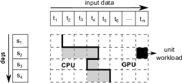
Figure 2: Fine-grained co-processing algorithm on a series of steps.

We can consider OL and DD as special cases for PL. DD is equivalent to PL with all the ratios the same on all steps. OL is equivalent to PL with all the workload ratios being either zero or one.

The co-processing schemes presented above outline an interesting design space for hash joins on the coupled architecture. In this experimental study, we focus on evaluating how those co-processing mechanisms are implemented in SHJ and PHJ.

We apply DD, OL and PL schemes to SHJ and obtain three variants (SHJ-DD, SHJ-OL and SHJ-PL, respectively). For each variant, we consider all $b_{i}$ ($1\leq i\leq 4$) in the build phase and all $p_{i}$ ($1\leq i\leq 4$) in the probe phase as two different step series. There are some tuning parameters, and we use the cost model presented in the next section to determine their suitable values for the best performance.

Some details of those SHJ variants are described as follows: (1) SHJ-DD: It decides two workload ratios, $r_{b}$ and $r_{p}$, $0\leq r_{b},r_{p}\leq 1$, for the build and the probe phases, respectively. For example, in the build phase, a portion of $r_{b}$ of the build table are processed by the CPU to construct the hash table. (2) SHJ-OL: It decides whether each of the steps ($b_{i}$ in the build phase and $p_{i}$ in the probe phase) is performed on the CPU or the GPU. (3) SHJ-PL: It determines the suitable workload ratios for all the steps in the build and the probe phases.

We apply DD, OL and PL schemes to PHJ and obtain three variants (PHJ-DD, PHJ-OL and PHJ-PL, respectively). The idea is the same as the above SHJ variants, except that we consider the steps in each pass of partitioning as a step series.

3.3 Implementations and Design Tradeoffs

There are a few design tradeoffs in memory optimizations and OpenCL-related optimizations, which often have significant impact on the performance of hash joins.

Memory allocator. In the hash join algorithm, dynamic memory allocations are common, including (1) the output buffer for a partition, (2) allocating a new key in the key list, and (3) the join result output. Current OpenCL (version 1.2) does not support dynamic memory allocation inside the kernel. The efficiency in supporting dynamic memory allocations is essential for those operations. Inspired by the previous study [20], we develop a software dynamic memory allocator on a pre-allocated array, and memory requests are dynamically allocated from that array.

A basic implementation of the memory allocator is to use a single pointer marking the starting address of the free memory in an pre-allocated array. The pointer initially points to the starting address of the array. After serving a memory request, the pointer is moved accordingly. We use the atomic operation (specifically atomic_add in our study) to implement a latch for synchronization among multiple requests. Additionally, the latch is applicable at both the local memory and the global memory operations. However, this basic implementation could suffer from the contention of atomic operations, especially for supporting massive thread parallelism on the GPU.

To reduce the contention, we develop an optimized memory allocator. The memory allocation is at the granularity of a block. The block size is a tuning parameter and we will experimentally evaluate its impact in the experiments. The memory allocator maintains a global pointer. The memory request is always made by work item 0 (Thread 0) from a work group, and the global pointer is advanced by one block size. The memory allocator returns one block to the work group. The threads within the work group request memory from the block. It uses a local pointer for synchronization among the threads within the work group. We allocate the local pointer in the local memory to reduce the memory access overhead. Note, the local memory is accessible to all the threads within a work group.

The optimized memory allocator resolves the contention on the GPU. Additionally, the pre-allocation is also beneficial for the CPU. It eliminates many small malloc operations, and reduces the memory allocation overhead on the CPU.

Shared vs. separate hash tables. Cache performance and concurrency are two key factors for the design of hash tables. An important design choice in the build phase is to use a shared hash table or separate hash tables for the CPU and the GPU. Either solution has its own benefits and drawbacks. A shared hash table has better cache performance, since the CPU and the GPU share the data cache on the coupled architecture. Additionally, it uses less memory space in the zero copy buffer. On the other hand, separate hash tables have smaller latch contention between the CPU and the GPU. We experimentally evaluate these two solutions.

Workload divergence. In OpenCL, all work items in the same wavefront run simultaneously in a lockstep. The execution time of a wavefront is equal to the worst execution time of all work items. Workload divergence among work items causes severe penalties in the overall performance of the wavefront. One common source of workload divergence in hash joins is data skew. For example, data skews cause workload divergence in $b_{3}$ in the build phase and $p_{3}$ in the probe phase.

To reduce the workload divergence, we adopt a grouping-based approach in the previous study [18], which is used to reduce the branch divergence of transaction executions on the GPU. In order to reduce the workload divergence, we group the input data according to the amount of workload. Using the probe as an example, the input data are the hash bucket headers given in $b_{2}$, and the amount of workload is represented by the number of keys in the key list. After grouping, the input data with the similar amount of workload are grouped together, and the divergence among the work items in a work group is reduced. The number of groups is tuned for the tradeoff between the grouping overhead and the gain of reduced workload divergence.

Step definitions. So far, we have adopted very fine-grained step definitions for co-processing. Ideally, there are other granularities of defining steps, which can have different memory performance and efficiency of co-processing.

We are particularly interested in evaluating the step definition for PHJ in the previous study [4]. After the partition phase, we have got $P$ partition pairs on $R$ and $S$ ($<$$R_{i}$, $S_{i}$$>$, $0\leq i\leq{P-1}$). The further join processing on $R_{i}$ and $S_{i}$ is performed by one thread. Thus, all the join processing on the $P$ partition pairs on $R$ and $S$ can be viewed as a step, and a partition pair is considered to be the input data item to the step. Thus, the granularity for a step for this co-processing is a SHJ on the partition pair. Note, those SHJs use separate hash tables, which potentially loses the opportunities of cache reuse in our fine-grained PHJ variants.

4 Performance Model

There are a number of parameters (for example, the ratio in the data-dividing scheme) to be determined for the co-processing performance on the coupled architecture. In this section, we develop a cost model to predict the performance of hash joins with co-processing on the coupled architecture, and then use the cost model to determine the suitable values for the parameters.

Cost models for hash joins have been developed in previous studies, e.g., on the CPU [5, 26] and the GPU [15]. Those cost models are highly specialized for the target architectures and the architecture-specific query processing algorithms. For example, the cost model for GPU-based co-processing [15] needs the cost estimation on the PCI-e data transfer. In this study, the implementations on the CPU and the GPU are based on the same OpenCL programs with different input parameters. The CPU and the GPU are abstracted as the same compute device model. Moreover, the CPU and the GPU share the data cache and the main memory without the PCI-e bus on the coupled architecture. It is desirable to have an unified model to estimate the performance of co-processing on both the CPU and the GPU in terms of both computation and memory latency.

Table 2: Notations in the cost model

Notation	Description
$r_{i}$	Workload ratios for the CPU at Step $i$ ($1\leq i\leq\#\mathit{Steps}$)
$x_{i}$	The number of input items (e.g., tuples) at Step $i$ ($1\leq i\leq\#\mathit{Steps}$)
$T$	Total elapsed time of executing the entire step series
$T_{\mathit{XPU}}$	The execution time on the processor $\mathit{XPU}$ ($\mathit{XPU}=\{\mathit{CPU},\mathit{GPU}\}$)
$T^{i}_{\mathit{XPU}}$	The execution time on the processor $\mathit{XPU}$ at Step $i$
$C^{i}_{\mathit{XPU}}$	Computation time at Step $i$
$M^{i}_{\mathit{XPU}}$	Total global memory access time at Step $i$
$D^{i}_{\mathit{XPU}}$	The pipelined delay at Step $i$
$\#\mathit{I}^{i}_{\mathit{XPU}}$	The average number of instructions on $\mathit{XPU}$ per tuple in Step $i$
$\mathit{IPC}_{\mathit{XPU}}$	The peak instruction per cycle on $\mathit{XPU}$

In Section 3, we have identified PL as a basic abstraction for hash join co-processing on the coupled architecture (DD and OL are special cases for PL). This allows us to abstract the common design issues on the cost model for different co-processing schemes. We call this high level abstraction the abstract model. For a specific co-processing algorithm, we obtain its cost model by instantiating the abstract model with profiling and algorithm-specific analytic modelling (e.g., memory optimizations). In the remainder of this section, we first present the abstract model for PL on the coupled architecture, and next use SHJs as an example of instantiating the abstract model.

4.1 The Abstract Model

We model the elapsed time of executing a step series with PL. The step series consists of $n$ steps, with $x_{i}$ input data items on Step $i$ ($1\leq i\leq n$). The cost model predicts the elapsed time of PL with workload ratios $r_{i}$ in Step $i$. The parameters are summarized in Table 2 for reference. Thus, the total elapsed time $T$ is estimated to be the longer execution time of the CPU and the GPU.

$$T=max(T_{\mathit{XPU}}),\mathit{XPU}=\{\mathit{CPU},\mathit{GPU}\}$$ (1)

On each processor, we estimate the execution time to be the total execution time of all steps in the step series. The execution time of Step $i$ ($T^{i}_{\mathit{XPU}}$) is further estimated in three parts: computation time $C^{i}_{\mathit{XPU}}$, global memory access time $M^{i}_{\mathit{XPU}}$ and the pipelined delay $D^{i}_{\mathit{XPU}}$.

$$T_{\mathit{XPU}}=\sum\limits_{i=1}^{n}T^{i}_{\mathit{XPU}}=\sum\limits_{i=1}^{n}(C^{i}_{\mathit{XPU}}+M^{i}_{\mathit{XPU}}+D^{i}_{\mathit{XPU}})$$ (2)

We describe the estimation of each component accordingly.

We estimate the computation time to be the total execution time for all the instructions of the step. We assume an ideal execution pipeline with the optimal IPC on each processor, and a hash join on uniform data distributions.

$$C^{i}_{\mathit{XPU}}=\frac{\#\mathit{I}^{i}_{\mathit{XPU}}\times r_{i}\times x_{i}}{\mathit{IPC}_{\mathit{XPU}}}$$ (3)

To estimate the memory stalls, we adopt a traditional calibration method for the CPU [26] and for the GPU [15], which can estimate the memory stall cost per data item in each step. The basic idea is to measure the memory stall cost, by excluding the caching effects and the thread parallelism. It is suitable to estimate the memory stall costs for both random and sequential accesses. For details on the calibrations and models, we refer readers to the original paper [15, 26]. For different steps, we have instantiated the model with the consideration of their access patterns.

For $D^{i}_{\mathit{XPU}}$, this delay is caused by different workload ratios in the two consecutive steps. Due to data dependency between the two processors, one processor has to synchronize with the other one on Step $i$ if the workload ratios are different on Steps $i$ and $(i-1)$. The delay occurs when the input data for Step $i$ have not been generated from Step $(i-1)$. There are two cases depending on the workload ratio comparison.

Case 1: if $r_{i}>r_{i-1}$, we use Eq. 4. The CPU may encounter delay while the GPU prepares the input data in Step $(i-1)$ for the CPU in Step $i$. The ratio of the GPU time that is not pipelined with the CPU in Step $(i-1)$ is $\frac{1-r_{i}}{1-r_{i-1}}$. By subtracting this amount of time ($T^{i-1}_{GPU}\times\frac{1-r_{i}}{1-r_{i-1}}$) from the total GPU time from Step $1$ to Step $i-1$, we get the time of the GPU from Step $1$ to the end of the pipelined execution area in Step $i-1$. The total CPU time from Step $1$ to the end of pipelined execution area with the GPU in Step $i$ is $\sum\limits_{j=1}^{i}T^{j}_{\mathit{CPU}}$. Therefore, $D^{i}_{CPU}$ is the delay time on the CPU to wait for data generated from the GPU in Step $i-1$, as in Eq. 4. Naturally, if $D^{i}_{CPU}\leq 0$, it is set as 0, meaning there will be no pipelined execution delay.

$$\begin{split}D^{i}_{\mathit{CPU}}=(\sum\limits_{j=1}^{i-1}T^{j}_{\mathit{GPU}}-T^{i-1}_{GPU}\times\frac{1-r_{i}}{1-r_{i-1}})-\sum\limits_{j=1}^{i}T^{j}_{\mathit{CPU}}\end{split}$$ (4)

Case 2: If $r_{i}<r_{i-1}$, we use Eq. 5 to calculate the pipelined execution delay for the GPU in a similar way to Case 1.

$$\begin{split}D^{i}_{\mathit{GPU}}=&\sum\limits_{j=1}^{i-1}T^{j}_{\mathit{CPU}}-(\sum\limits_{j=1}^{i}T^{j}_{\mathit{GPU}}-T^{i}_{\mathit{GPU}}\times\frac{1-r_{i-1}}{1-r_{i}})\end{split}$$ (5)

Finally, as specific to the pipelined co-processing, we need to estimate the cost of intermediate results and the communication cost between the CPU and the GPU. We estimate the cost for two consecutive steps. If they have the same workload ratio, we can ignore the costs on intermediate results and the communication. Otherwise, the amount of intermediate results can be derived from the difference of the workload ratio between the two steps. For Step $i$, the number of intermediate data items is $(r_{i}-r_{i-1})\times x_{i}$, assuming a uniform distribution.

4.2 Model Instantiation

We use SHJs as an example to illustrate the model instantiation. We consider fine-grained co-processing SHJ variants (with the granularity of tuples).

For computation time, the optimal IPC value can be obtained from the hardware specification. The number of instructions for per tuple in each step can be obtained from profiling tools such as AMD CodeXL and AMD APP Profiler. One issue to handle is that the number of instructions per tuple in some steps varies with the workload. For example, the costs of $b_{3}$ and $p_{3}$ depend on the length of the key list. Therefore, we use the number of instructions per key search as the unit cost for that step, and estimate the number of instructions of the step to be the number of instructions per key search multiplied by the average number of keys in the key list.

Next, we calibrate the memory unit cost per tuple with the calibration method [15]. For some steps, the memory unit cost is workload-dependent. We adopt the same approach as profiling the number of instructions discussed above.

Given the above calibrations, we can derive the total cost for different SHJ variants. Here, we use SHJ-DD as an example, and we can derive the cost for other variants similarly. We estimate the performance of SHJ-DD as the total elapsed time of the build phase and the probe phase. Since the estimation of the build phase is similar to the probe phase, we estimate the build phase as follows. We instantiate Eqs. 1–5. In Eq. 2, we set $n=4$, because there are four steps in the build phase. In Eq. 3, the number of instructions is substituted with the profiled result from each step. We then use the calibrated values for each step to get the memory costs, and determine the pipelined execution delay in Eqs. 4 and 5. Thus, we can get the cost for the build phase in Eq. 1.

5 Evaluation

In section, we experimentally evaluate the co-processing scheme for the hash join on the coupled CPU-GPU architecture. Overall, there are four groups of experiments. Firstly, we investigate the overhead of data transfers and other operations of co-processing for the hash join on a discrete CPU-GPU architecture (Section 5.2). Secondly, we evaluate the accuracy of our cost model (Section 5.3). Thirdly, we study the performance impact of the design tradeoffs in co-processing of hash joins (Section 5.4). Finally, we show the end-to-end performance comparison (Section 5.5).

5.1 Experimental Setup

Hardware configuration. We conduct our experiments on a PC equipped with an AMD APU A8-3870K. The hardware specification has been summarized in Table 1.

Data sets. We use the same synthetic data sets as the previous study [4] to evaluate our implementations. Both relations $R$ and $S$ consist of two four-byte integer attributes, namely the record ID and key value. Our default data set size is 16 million tuples with uniform-distributed key values for both relations $R$ and $S$, unless specified otherwise. Both $R$ and $S$ can be considered as basic relations (without compression) in column-oriented databases, or the intermediate relations by extracting the key and record ID from much larger relations in row-oriented databases. We experimentally evaluate the impact of different data sizes. In addition to uniform data sets, we also use skewed data sets and vary the selectivity to show the overall performance comparisons. We created two skewed datasets with $s\%$ of tuples with one duplicate key values: low-skew with $s=10$ and high-skew with $s=25$.

Implementation details. We develop all hash join variants using OpenCL 1.2. The OpenCL configuration including work groups and work items has been tuned to fully utilize the CPU and the GPU capabilities. In addition to co-processing, we also implement CPU-only and GPU-only algorithms. Our implementations have adopted the common practice in the previous implementations [17, 4, 5]. For example, we choose the hash function MurmurHash 2.0 that is also used in the previous study [4], which has a good hash collision rate and low computational overhead.

We compare the discrete and the coupled architectures to investigate the performance issues of discrete architectures. For a fair comparison, we should ideally use the CPU and the GPU that have exactly the same architectures as those in the coupled architecture. However, this may be not always feasible as the coupled architecture advances. Instead, we use the CPU and the GPU on the coupled architecture to emulate the CPU and the GPU on a discrete architecture, and emulate the PCI-e bus data transfer with a delay. This simulation-based approach allows us to evaluate the impact of different processors and PCI-e bus. Unlike real discrete architectures, the CPU and the GPU in the emulated architecture still share the cache. In our experiment, we find that the emulated approach is able to help us to understand the performance issues of the discrete architecture. The delay of one data transfer on PCI-e bus is estimated to be $\mathit{latency}+\frac{\mathit{size}}{\mathit{bandwidth}}$, where $\mathit{size}$ is the data size and $\mathit{latency}$ and $\mathit{bandwidth}$ are the latency and bandwidth of the PCI-e bus, respectively. In our study, we emulate a PCI-e bus with $\mathit{latency}=0.015$ ms and $\mathit{bandwidth}=3$ GB/sec.

On the emulated discrete architecture, we can implement all the hash join variants except PL. Using SHJ-DD as an example, in the build phase, a part of the build table is transferred to the GPU memory before the GPU starts building hash tables. An estimated delay is added so that the GPU starts the build phase later. When the build phase is done, the partial hash table is transferred back to the CPU for a merge operation. The probe phase has a similar process to the build phase. For PL, it is inefficient to implement the fine-grained co-processing on the discrete architecture for two reasons. Firstly, there are much more memory data transfers by exchanging the intermediate results between the CPU and the GPU. Secondly, the data dependency control logic on the GPU memory is difficult to implement on the PCI-e bus. Thus, we use the execution of PL on the coupled architecture to analyse the impact of PL on the discrete architecture, including intermediate results and efficiency of pipelined execution.

5.2 Evaluations on Discrete Architectures

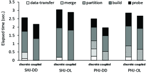
Figure 3: Time breakdown on discrete and coupled architectures

Data transfer and merge overhead. We first study the time breakdown of hash join variants on the discrete architecture. For comparison, we also show the time breakdown on the coupled architecture. Figure 3 shows the time breakdown for the data dividing and off-loading co-processing schemes. On the discrete architecture, the workload ratios for the build and probe phases for SHJ-DD are 25% and 42%, respectively; the workload ratios for the partition, build and probe phases for PHJ-DD are 11%, 26% and 41%, respectively. We can see that the suitable workload ratios vary across different phases. SHJ-OL and PHJ-OL have degraded to be GPU-only, because all the steps on the GPU are faster than those on the CPU (as we will discussed later).

On the discrete architecture, co-processing usually requires explicit data transfer on the PCI-e bus and the merge operation. In the experiments, DD has both kinds of overhead and OL has only the data transfer overhead because OL is essentially GPU-only. Overall, the PCI-e data transfer overhead is 4–10% of the overall execution time. PHJ generally has higher data transfer overhead, since it has one more phase than SHJ. In comparison, this data transfer overhead is eliminated on the coupled CPU-GPU architecture.

The merging operation usually creates a more significant overhead than the data transfer on PCI-e bus (14% and 18% of the overall time in SHJ-DD and PHJ-DD, respectively). While the data transfer overhead on the PCI-e bus can be reduced with advanced overlapping of computation and data transfer, the merge overhead is inherent to DD on the discrete architecture. In comparison, on the coupled architecture, DD uses a shared hash table (as we evaluate in Section 5.4), and the merge overhead is eliminated.

Workload ratios in DD. We study the workload ratios on two different architectures (Figures are omitted due to space limits). Generally, we find that the suitable workload ratios of the CPU on the discrete architectures are higher than those on the coupled architecture. During the data transfer, the CPU can do more useful work for DD. Since the data transfer accounts for 4–10% of the total execution time, the difference is small (smaller than 5%).

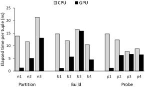
Figure 4: Unit costs for different steps on the CPU and the GPU for PHJ

GPU and CPU processing capabilities for different steps. In order to achieve the efficiency of employing fine-grained co-processing, we need to understand the processing performance of each step on the CPU and the GPU. We measure the performance of each step on the CPU-only and the GPU-only algorithms. Figure 4 shows the average processing time per tuple for different steps in PHJ on the CPU and the GPU. We have observed similar results on SHJ. Overall, the hash value computation can greatly benefit from the GPU acceleration due to its massive data parallelism and computation intensity. Therefore, the GPU can accelerate the hash value computation based steps (i.e., $n_{1}$, $b_{1}$, and $p_{1}$) by more than 15X. Instead, some other operations, such as $b_{3}$ or $p_{3}$, cannot match the GPU architecture features, because of random memory accesses and divergent branches. As a result, the GPU and the CPU have very close performance on those steps. Since different steps may have different performance comparison on the CPU and the GPU, this confirms that a fine-grained co-processing algorithm is essential to better exploit the strength of the CPU and the GPU. Workloads of different steps should be carefully assigned to suitable compute devices. That leads to our further analysis of PL.

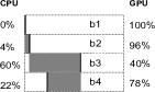
(a) build in SHJ

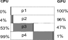
(b) probe in SHJ

Figure 5: Optimal workload ratios of different steps for SHJ-PL on the coupled architecture

(a) partition in PHJ

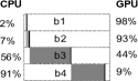
(b) build in PHJ

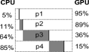
(c) probe in PHJ

Figure 6: Optimal workload ratios of different steps for PHJ-PL on the coupled architecture

Analyzing PL. We analyze the workload ratios of different steps for PL on the coupled architecture to understand the impact of intermediate results and efficiency of pipelined execution. Figures 5 and 6 show the optimal workload ratios of different steps in SHJ-PL and PHJ-PL on the coupled architecture, respectively. Overall, the optimal workload ratios are varied across different steps. The GPU can take all workload ($b_{1}$ in Figure 5(a) and $p_{1}$ in Figure 5(b)), or takes only a very small portion of workload (1% for $p_{4}$ in Figure 5(b)). We have the following two implications.

Firstly, PL can be inefficient on the discrete architecture, since the significant difference in the workload ratios among the steps creates significant overhead in data transfer and pipeline execution. Recall that, in PL, the workload ratio difference between two consecutive steps determines the amount of intermediate results. We use the grey area in the figures to indicate the intermediate results to be generated during the execution of PL. For example, in Figure 5, the CPU only takes 4% workload for $b_{2}$, but takes 60% for $b_{3}$. That requires a transfer of 56% of the output data of $b_{2}$ on the PCI-e bus, if PL runs on the discrete architecture. On the other hand, the overhead of pipelined execution is not shown in the figure. The difference in the workload ratios results in different lengths of pipelines in the execution, which results in workload divergence.

The other implication is that, since the optimal workload ratios vary for different steps, the conventional approach (by offloading the entire join to the GPU) cannot fully exploit the co-processing capabilities from both the CPU and the GPU.

5.3 Cost Model Evaluation

Overall, our cost model can accurately predict the performance of all hash join variants with different tuning parameters, and thus can guide the decision of getting the suitable value. Since the results are similar for both SHJs and PHJs, we focus of the results on SHJs.

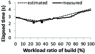
(a) build

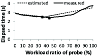
(b) probe

Figure 7: Estimated and measured time for SHJ-DD with workload ratios varied

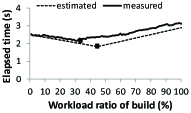
(a) build

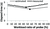
(b) probe

Figure 8: Estimated and measured time for a special case for PL: offloading entire $b_{1}$ and $p_{1}$ to the GPU, and applying data-dividing with the same ratio $r$ to all the other steps. The results are measured by varying $r$.

Figure 7 compares the estimated performance with measured performance for SHJ-DD with the workload ratios varied. The black solid squares in the figures denote the optimal points. It shows that our estimated time is close to the measured time. However, the estimated time is slightly lower than the measured time. One factor to consider is that our cost model does not include the estimation of the lock contention overhead.

PL has a large design space. In general, our estimation can closely predict the performance of PL with different workload ratios. For clarity of presentation, we consider a special case for PL: offloading the entire $b_{1}$ and $p_{1}$ to the GPU, and applying data-dividing with the same ratio $r$ to all the other steps. The results in Figure 8 are measured by varying $r$. In this special case of PL, we see that our prediction is close to the performance varying $r$ and also is able to predict its suitable value.

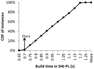
(a) build of SHJ-PL

(b) probe of PHJ-PL

Figure 9: CDF of SHJ-PL (build) and PHJ-PL (probe) with one thousand Monte Carlo simulations

To evaluate our cost model in more details, we perform experiments with Monte Carlo simulations on the workload ratios. Each simulation runs a PL with randomly generated ratio settings. Figure 9 demonstrates the cumulative distribution function (CDF) for the elapsed time of the build phase of SHJ-PL and the probe phase of PHJ-PL with one thousand simulation runs. We also highlight the elapsed time of our approach given by the cost model. The proposed approach is very close to the best performance of the Monte Carlo simulations. For each simulation run, we evaluate the prediction by our model and the measured execution time. The difference is smaller than $15\%$ in most cases.

5.4 Design Tradeoffs on Coupled CPU-GPU Architectures

We evaluate the impact of each tradeoff by varying the setting of that tradeoff while other tradeoffs have already been tuned. Based on them, we optimize the performance of the hash join variants on the target coupled architecture.

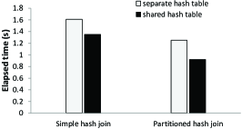
Figure 10: Elapsed time of the build phase in DD with separate and shared hash tables

Separate vs. shared hash table. We first show the elapsed time of build phase of DD with separate and shared hash tables, as shown in Figure 10. SHJ-DD and PHJ-DD with a shared hash table outperform those with separate hash tables by 16% and 26%, respectively. The major benefit of adopting the shared hash table is the elimination of the merging operation (as we have seen in Section 5.2). The other benefit is the improved cache performance due to potential cache reuse on the coupled architecture. The numbers of cache misses of SHJ-DD and PHJ-DD with separate hash tables are 2% and 4% larger than those with shared hash table, respectively. The improvement shows that, on the tested coupled architecture, the concurrency overhead of the shared hash table is compensated by the two major benefits over the separate hash table.

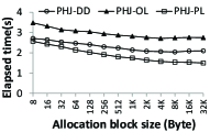
(a) Elapsed time (sec.)

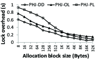
(b) Lock overhead

Figure 11: Elapsed time (left) and lock overhead (right) of PHJ

Optimized memory allocator. We adopt an optimized memory allocator to reduce the number of atomic operations. Figure 11(a) shows the overall time with the memory allocation block size varied in PHJ. We observed similar results on SHJ. Overall, at the beginning, the performance keeps improving when the block size becomes larger. However, the performance remains stable when the block size is larger than 2KB. The suitable block size is set to 2KB in our experiments. The major reason of the performance improvement is the reduction of global memory lock overhead from atomic operations.

To confirm our conclusion, we further study the lock overhead with the block size varied in Figure 11(b) for PHJ. So far, there is no profiling tool to measure the lock overhead directly on the hardware. Therefore, we estimate the lock overhead as the difference of the measured time and estimated time based on our cost model. This is because our cost model does not consider the lock overhead. This back-of-the-envelop approach is simplistic but sufficient to show the trend of the lock overhead for our purpose. As the allocation memory block size increases, the lock overhead decreases significantly for all hash join variants.

Figure 12 compares the performance of hash joins with the basic memory allocator and our optimized memory allocator (denoted as Basic and Ours, respectively). Compared with the Basic allocator, the optimized allocator significantly improves the hash join performance, with up to 36% and 39% improvement on SHJ and PHJ.

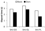
(a) SHJ

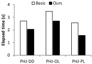
(b) PHJ

Figure 12: Comparison between basic and optimized memory allocators (Basic and Ours, respectively)

Workload divergence. We study the impact of grouping approach on reducing the workload divergence. Our experimental results show that, the grouping approach can improve the overall performance by 5–10% (Figures are omitted due to space interests). The impact on the GPU is larger than that on the CPU, because the GPU hardware executes the wavefront strictly in a SIMD manner and also does not have advanced branch prediction mechanisms like the CPU.

Fine-grained step definition. We study the CPU and the GPU running time for hash joins employing the fine-grained and coarse-grained step definition. We apply PL to the coarse-grained step definition that we discussed in Section 3.3, and denote this co-processing to be PHJ-PL’. Table 3 shows the execution time and the cache performance of PHJ-PL and PHJ-PL’. PHJ-PL’ is much slower than PHJ-PL. As the coarse-grained step definition introduces separate hash tables, PHJ-PL’ has a larger number of cache misses and a higher cache miss ratio than PHJ-PL. This shows the advantage of co-processing with fine-grained steps.

Table 3: Comparison between fine-grained and coarse-grained step definitions in PL

	L2 cache misses ($\times 10^{6}$)	L2 cache miss ratio	Time (s)
PHJ-PL	7	10%	1.6
PHJ-PL’	15	23%	2.2

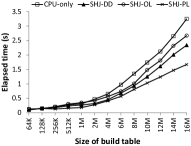
(a) SHJ

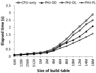
(b) PHJ

Figure 13: Elapsed time comparison on the uniform data set

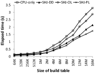
(a) SHJ

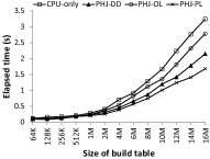
(b) PHJ

Figure 14: Elapsed time comparison on the high-skew data set

5.5 End-to-End Performance Comparison

In this section, we compare end-to-end performance for different hash join variants on the coupled architecture. The OL essentially is a GPU-only implementation, and thus the results for GPU-only are omitted.

Data skew and data size. We first show performance numbers on the uniform, low-skew and high-skew data sets. We fix the probe relation to 16 million tuples and vary the build relation from 64K to 16M tuples. Figures 13 and 14 show the comparison results for uniform and high-skew data sets, respectively. The figures for the low-skew data sets are omitted due to the space limits, and we describe the results in texts. In general, they have similar performance trends on all three data sets. It shows that our co-processing techniques work well on either uniform or skew data sets. The elapsed time of running on high-skew data can be actually comparable to or even lower than that on uniform data. This is mainly because the benefit of data locality in high-skew data compensates the overhead of latches. This point has also been pointed out in the previous study [4]. We have also observed that when the relation size exceeds the cache size (4MB), there is a leap in the running time. Additionally, the performance improvement also scales well with the build relation size. In most cases, exploiting the capabilities of the both the GPU and the CPU (DD and Pipelined) can generate better performance than using only the CPU (CPU-only) or GPU-only (OL). Specifically, the optimized fine-grained pipelined join outperforms the CPU-only and GPU-only implementations by up to 53% and 35%, respectively. Thus, it is important to exploit both the CPU and the GPU on the coupled architecture. Additionally, PL outperforms DD by up to 28%. This confirms the effectiveness of our optimizations on fine-grained co-processing.

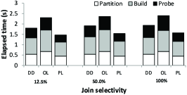
Figure 15: PHJ with join selectivity varied

Join selectivity. We study the impact of join selectivity. Figure 15 shows the results on time breakdown for the join selectivity values of 12.5%, 50% and 100%. For DD and OL, the selectivity only affects the probe phase. As a result, the time for the probe phase becomes slightly longer when the selectivity increases from 12.5 % to 100% for DD (from 0.47 to 0.58 seconds) or OL (from 0.59 to 0.71 seconds). For PL, both the build and probe phases are affected by the join selectivity. However, the performance impact is marginal, because our implementation simply outputs the matching $\mathit{rid}$ pair. When the selectivity increases, there are more chances for workload divergence when probing the hash table.

After studying all hash join variants, we find that PHJ-PL is usually the fastest, which is 2–6% faster than SHJ-PL. Nevertheless, both SHJ-PL and PHJ-PL are very competitive on the coupled architecture on different data sets.

5.6 Summary and Lessons Learnt

We summarize the major findings and lessons learnt from this study and their implications for developing an efficient query processor on the coupled architecture.

Firstly, conventional co-processing of hash joins [17, 22] can achieve only marginal performance improvement on the coupled architecture, since only the data transfer overhead is eliminated (accounting for 4–10% of the total execution time). This calls for the use of fine-grained co-processing on the coupled architecture, instead of coarse-grained co-processing in the previous studies [15, 12, 17]. Moreover, fine-grained co-processing schemes are inefficient on the discrete architecture. It indicates that “one size does not fit all”, and we need to adopt different co-processing schemes between discrete and coupled architectures.

Secondly, fine-grained co-processing on hash joins has an interesting design space. It further increases the number of tuning knobs for hash joins. Automaticity of optimization is feasible which is enabled by our cost model. Going beyond hash joins, we believe that the automaticity could be achieved through integrating the awareness of fine-grained co-processing into query optimizations.

Thirdly, memory optimizations and OpenCL-related optimizations have significant impact on the overall performance of hash join co-processing. Traditional issues like shared vs. separate hash tables remain important on the coupled architecture. More generally, architecture-aware query processing techniques (e.g., [3, 29]) are still relevant to performance optimizations. But their impacts should be carefully studied on the target coupled architecture.

Fourthly, fine-grained co-processing is a must on the coupled architecture, which significantly outperforms the performance of processing on a single processor and the conventional co-processing. It not only keeps both processors busy, but also assigns the suitable workload to them for efficiency. The design space applies to general query processing, and an efficient query processor should expose sufficiently fine-grained data parallelism for scheduling among different processors. Additionally, we conjecture that the design space of co-processing in this study is relevant to not only the coupled CPU-GPU architectures but also other heterogeneous architectures [23].

6 Conclusion

While GPU co-processing has shown significant performance speedups on main memory databases, the discrete CPU-GPU architecture design has hindered the further performance improvement of GPU co-processing. This paper revisits co-processing for hash joins on the coupled CPU-GPU architecture. With the integration of the CPU and the GPU into a single chip, the data transfer via PCI-e bus is eliminated on the coupled architecture. More importantly, the coupled architecture has opened up vast opportunities for improving the performance of co-processing of hash joins, as we have demonstrated in this experimental study. Specifically, we revisit the design space of fine-grained co-processing on hash joins with and without partitioning. We show that the fine-grained co-processing can improve the performance by up to 53%, 35% and 28% over the CPU-only, GPU-only and conventional CPU-GPU co-processing, respectively. This paper represents a key first step in designing efficient query co-processing on coupled architectures. We are developing a full-fledged query processor on the coupled architecture [36].

7 Acknowledgement

The authors would like to thank anonymous reviewers, Qiong Luo and Ong Zhong Liang for their valuable comments. This work is partly supported by a MoE AcRF Tier 2 grant (MOE2012-T2-2-067) in Singapore and an Inter-disciplinary Strategic Competitive Fund of Nanyang Technological University 2011 for “C3: Cloud-Assisted Green Computing at NTU Campus”.

Appendix A More Experimental Results

We present more experimental results, including comparison with a coarse-grained scheduling approach, evaluating hash join performance for data sets larger than zero copy buffer and more detailed studies on latches.

Comparison with A Coarse-Grained Scheduling Approach. For comparison, we have implemented a simple coarse-grained scheduling approach (namely “BasicUnit”). The BasicUnit approach dynamically assigns a chunk of tuples to the CPU or the GPU, and performs the build or probe operations with that chunk on the corresponding processor. Due to the architectural difference between the CPU and the GPU, the chunk size is tuned for the target architecture. Compared with our proposed approach, the BasicUnit approach has a major deficiency: the CPU may perform more non-CPU-optimized tasks than our proposed fine-grained co-processing, and vice versa. We have implemented the suggested approach, and report the results in Figure 16. When both R and S tables have 16M tuples, our proposed approaches (SHJ-PL and PHJ-PL) are 31% and 25% faster than their counterparts using the BasicUnit approach. Besides, although BasicUnit works like DD, the scheduling overhead of BasicUnit results in performance degradation.

We have further investigated the workload ratios of different steps on the CPU and the GPU. Figures 17 and 18 show the results using the BasicUnit approach for SHJ and PHJ, respectively. The ratios are significantly different from the optimal ratios given by our cost model (Figures 5 and 6 in the paper) because the CPU or the GPU has to process the same portion of the workload in all steps of a given phase, resulting in deficiency compared with our fine-grained co-processing.

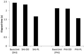
Figure 16: Performance comparison between BasicUnit and fine-grained co-processing algorithms

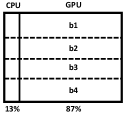
(a) Build

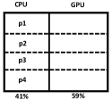
(b) Probe

Figure 17: Workload ratios of different steps for SHJ employing BasicUnit

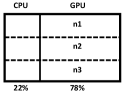
(a) Partition

(b) Build

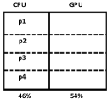
(c) Probe

Figure 18: Workload ratios of different steps for PHJ employing BasicUnit

Large datasets that cannot fit into the zero copy buffer. In the current system, the zero copy buffer size is limited. For larger data sets that cannot fit into the zero copy buffer, we perform the hash join with partitioning. The algorithm is similar to classic hash joins for external memory. Here, we view the zero copy buffer as main memory and other system memory as external memory. Specifically, we partition the build and the probe relations so that the join of a partition pair can fit into zero copy buffer. The partitioning can have multiple passes. In partition phase, a block of tuples from the input relation is partitioned in the zero copy buffer with our current partitioning algorithm. In our experiment, the chunk size is 16 million tuples. Next, we copy the intermediate partitions out from the zero copy buffer to the system memory. After all the inputs are partitioned, we link all the intermediate partitions together to form the result partition pairs. Next, we apply the hash join algorithms proposed in this paper to handle the join in each partition pair.

Figure 19 shows the performance when we vary the number of tuples in both relations $R$ and $S$ from 16M (256MB) to 128M (2GB). We compare different join algorithms on the partition pair, either SHJ-PL or PHJ-PL. PHJ-PL is up to 9% faster than SHJ-PL. We divide the elapsed time into three parts: data copy time, partition time and join time for the time on data transfer between the system memory and zero copy buffer, the time for partitioning and for performing the join on the partition pairs, respectively. There is no data copy time or partition time when $|R|=|S|=16M$, because the entire join can fit into the zero copy buffer. On other cases, partition time is very significant. We obtain the data copy time from AMD CodeAnalyst profiler. The data copy time is around 4% of the total time. Furthermore, both the partition time and the join time increase almost linearly with the size of input tables. It indicates good scalability of our algorithm when the data size is larger than zero copy buffer.

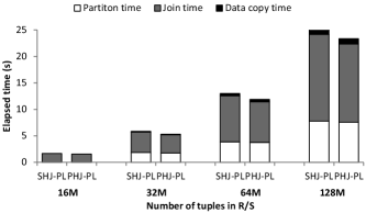
Figure 19: Comparing elapsed time of different join algorithms on each partition pair for large data sets ($|R|=|S|$)

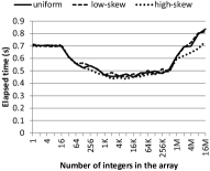
(a) Locking time on the CPU

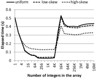
(b) Locking time on the GPU

Figure 20: The performance of micro benchmark on locking overhead on the CPU and the GPU

Locking overhead. We have designed a micro benchmark to study the performance impact of our latch implementation on APU. In the micro benchmark, we first generated an array of $N$ integers and then we used $K$ threads to perform $X$ increments in total on the array, where $X$ is a constant. The increment operation is implemented with our latch. We investigated different data distributions (the notations of “uniform”, “low-skew” and “high-skew” have the same meanings as the experimental setting in the paper). The results are shown in Figure 20, where $N$ ranges from 1 to 16M, $X$ is fixed to be 16M on both the CPU and the GPU, $K$ is fixed to be 8192 and 256 on the GPU and the CPU respectively. For both the CPU and the GPU, the overhead decreases when the data size increases until the input array cannot fit into the cache size (4MB). After that, the execution time of running on the high-skew data is slightly lower than that on the uniform data. This is mainly because of the benefit of data locality in the high-skew data that compensates the overhead of latches. This point has also been pointed out in Section 4.4 of the previous study [4].

References

- [1] A. Ailamaki, D. J. DeWitt, M. D. Hill, and D. A. Wood. Dbmss on a modern processor: Where does time go? In VLDB, 1999.
- [2] AMD Corp. http://amddevcentral.com/afds/pages/default.aspx.
- [3] C. Balkesen, J. Teubner, G. Alonso, and M. T. Oszu. Main-memory hash joins on multi-core cpus: tunning to the underlying hardware. In ICDE, 2013.
- [4] S. Blanas, Y. Li, and J. M. Patel. Design and evaluation of main memory hash join algorithms for multi-core cpus. In SIGMOD, pages 37–48, 2011.
- [5] P. A. Boncz, S. Manegold, and M. L. Kersten. Database architecture optimized for the new bottleneck: Memory access. In VLDB, 1999.
- [6] L. Chen, X. Huo, and G. Agrawal. Accelerating mapreduce on a coupled cpu-gpu architecture. In SC, pages 25:1–25:11, 2012.
- [7] M.-S. Chen, M.-L. Lo, P. S. Yu, and H. C. Young. Using segmented right-deep trees for the execution of pipelined hash joins. In VLDB, pages 15–26, 1992.
- [8] S. Chen, A. Ailamaki, P. B. Gibbons, and T. C. Mowry. Improving hash join performance through prefetching. ACM Trans. Database Syst., 2007.
- [9] D. DeWitt and J. Gray. Parallel database systems: the future of high performance database systems. Commun. ACM, 1992.
- [10] D. J. DeWitt and R. H. Gerber. Multiprocessor hash-based join algorithms. In VLDB, pages 151–164, 1985.
- [11] J. Fang, A. L. Varbanescu, and H. Sips. A comprehensive performance comparison of cuda and opencl. In ICPP, 2011.
- [12] W. Fang, B. He, and Q. Luo. Database compression on graphics processors. Proc. VLDB Endow., pages 670–680, 2010.
- [13] P. Garcia and H. F. Korth. Pipelined hash-join on multithreaded architectures. In DaMoN, pages 1:1–1:8, 2007.
- [14] B. Gold, A. Ailamaki, L. Huston, and B. Falsafi. Accelerating database operators using a network processor. In DaMoN, 2005.
- [15] B. He, M. Lu, K. Yang, R. Fang, N. K. Govindaraju, Q. Luo, and P. V. Sander. Relational query coprocessing on graphics processors. ACM TODS, pages 21:1–21:39, 2009.
- [16] B. He and Q. Luo. Cache-oblivious databases: Limitations and opportunities. ACM Trans. Database Syst., pages 8:1–8:42, 2008.
- [17] B. He, K. Yang, R. Fang, M. Lu, N. Govindaraju, Q. Luo, and P. Sander. Relational joins on graphics processors. In SIGMOD, pages 511–524, 2008.
- [18] B. He and J. X. Yu. High-throughput transaction executions on graphics processors. Proc. VLDB Endow., pages 314–325, 2011.
- [19] T. H. Hetherington and et al. Characterizing and evaluating a key-value store application on heterogeneous cpu-gpu systems. In ISPASS, pages 88–98, 2012.
- [20] C. Hong, D. Chen, W. Chen, W. Zheng, and H. Lin. Mapcg: writing parallel program portable between cpu and gpu. In PACT, pages 217–226, 2010.
- [21] T. Kaldewey, G. Lohman, R. Mueller, and P. Volk. Gpu join processing revisited. In DaMoN, pages 55–62, 2012.
- [22] C. Kim and et al. Sort vs. hash revisited: fast join implementation on modern multi-core cpus. PVLDB, 2009.
- [23] R. Kumar, D. M. Tullsen, and N. P. Jouppi. Core architecture optimization for heterogeneous chip multiprocessors. In PACT, pages 23–32, 2006.
- [24] Y. Li, I. Pandis, R. Mueller, V. Raman, and G. Lohman. Numa-aware algorithms: the case of data shuffling. In CIDR, 2013.
- [25] M.-L. Lo, M.-S. S. Chen, C. V. Ravishankar, and P. S. Yu. On optimal processor allocation to support pipelined hash joins. In SIGMOD, pages 69–78, 1993.
- [26] S. Manegold, P. Boncz, and M. L. Kersten. Generic database cost models for hierarchical memory systems. In VLDB, pages 191–202, 2002.
- [27] S. Manegold, P. A. Boncz, and M. L. Kersten. What happens during a join? dissecting cpu and memory optimization effects. In VLDB, 2000.
- [28] H. Pirk, S. Manegold, and M. Kersten. Accelerating foreign-key joins using asymmetric memory channels. In ADMS, 2011.
- [29] K. Ross. Efficient hash probes on modern processors. In ICDE, pages 1297–1301, 2007.
- [30] D. A. Schneider and D. J. DeWitt. A performance evaluation of four parallel join algorithms in a shared-nothing multiprocessor environment. In SIGMOD, pages 110–121, 1989.
- [31] A. Shatdal, C. Kant, and J. F. Naughton. Cache conscious algorithms for relational query processing. In VLDB, 1994.
- [32] M. Stonebraker and et al. C-store: a column-oriented dbms. In VLDB, pages 553–564, 2005.
- [33] G. Tan, L. Li, S. Triechle, E. Phillips, Y. Bao, and N. Sun. Fast implementation of dgemm on fermi gpu. In SC, 2011.
- [34] J. Teubner and R. Mueller. How soccer players would do stream joins. In SIGMOD, pages 625–636, 2011.
- [35] K. Thouti and S.R.Sathe. Comparison of openmp and opencl parallel processing technologies. IJACSA, pages 56–161, 2012.
- [36] S. Zhang, J. He, B. He, and M. Lu. Omnidb: Towards portable and efficient query processing on parallel cpu/gpu architectures. In PVLDB, pages 1–4, 2013.