Helioseismology of Pre-Emerging Active Regions III: Statistical Analysis

Abstract

The subsurface properties of active regions prior to their appearance at the solar surface may shed light on the process of active region formation. Helioseismic holography has been applied to samples taken from two populations of regions on the Sun (pre-emergence and without emergence), each sample having over 100 members, that were selected to minimize systematic bias, as described in Paper I (Leka et al., 2012). Paper II (Birch et al., 2012) showed that there are statistically significant signatures in the average helioseismic properties that precede the formation of an active region. This paper describes a more detailed analysis of the samples of pre-emergence regions and regions without emergence, based on discriminant analysis. The property that is best able to distinguish the populations is found to be the surface magnetic field, even a day before the emergence time. However, after accounting for the correlations between the surface field and the quantities derived from helioseismology, there is still evidence of a helioseismic precursor to active region emergence that is present for at least a day prior to emergence.

1. Introduction

Models for the formation of solar active regions (AR) tend to fall into one of several classes, largely dependent on the volume in which strong magnetic fields are generated. In one of these, magnetic flux tubes generated near the base of the convection zone become buoyant and rise through the convection zone (for a review see Fan, 2009), with an active region emerging when a flux tube passes through the solar surface. Another possibility is that ARs are formed as the result of the coalescence of magnetic fields generated in the bulk of the convection zone or near the solar surface (Brandenburg, 2005, and references therein). Each of these scenarios has a distinct signature in the velocity of the plasma in the convection zone. Local helioseismology (Gizon & Birch, 2005; Gizon et al., 2010) potentially can be used to determine the subsurface dynamics associated with AR formation, and thus could provide evidence for or against either of these theories. This would also indirectly shed light on the location of the solar dynamo.

Previous studies of AR formation using local helioseismology have tended to focus on only a small number of regions (e.g., Braun, 1995; Chang et al., 1999; Jensen et al., 2001; Zharkov & Thompson, 2008; Kosovichev, 2009; Hartlep et al., 2011; Ilonidis et al., 2011). The small number of regions considered and the lack of a control group of areas of Sun where no active region was emerging make it difficult to identify any subsurface properties unique to the emergence of active regions. The exception to this is the study of Komm et al. (2009, 2011) that considered subsurface flows of a large sample of existing active regions undergoing episodes of magnetic flux emergence, compared with a control group of active regions that had comparatively constant flux. However, this study did not include the pre-emergence stage of active region formation.

The present study is based on applying helioseismic holography (Lindsey & Braun, 2000) to samples of over 100 areas of Sun where an active region subsequently emerged, and an equal number where no active region emerged. The selection of these regions was described in Leka et al. (2013) (Paper I), while an initial analysis of the travel-times inferred from helioseismic holography, focusing on the average travel-time shifts, was presented in Birch et al. (2013) (Paper II). It was found that there are statistically significant differences in the average travel-times, as well as in the surface magnetic flux, between the samples of pre-emergence areas and quiet sun areas. These included a reduction in the mean travel-time shift of a few tenths of a second, as well as spatially antisymmetric features in both the east-west and north-south travel-time differences. The antisymmetric features are qualitatively consistent with what would be expected from a flow converging on the site of emergence, although it appears that it is not a simple converging flow. One possible interpretation is that emergence preferentially occurs at the boundaries between supergranules. In this scenario, the emergence is not at the center of a converging flow, but between neighboring diverging flows. This could also account for the difference in the surface magnetic field, as flux tends to concentrate in the boundaries between supergranules.

As interesting as what was found in Paper II is what was not found: any signature of a strong retrograde flow, or any travel-time shifts greater than of order one second. Simulations of rising flux tubes (e.g., Fan, 2008) predict retrograde flows with magnitudes of order 100 m s^-1, while Ilonidis et al. (2011) found mean travel-time reductions of order 10 s. In both these cases, the results are much larger effects than were found in Paper II, but for layers in the sun significantly below the roughly 20 Mm maximum depth considered here. Thus it may be that there are significant changes in the emergence process between depths of approximately 60 Mm and 20 Mm.

In the present paper, we briefly review the selection of the data, and the analysis performed in the previous papers in this series before proceeding to an analysis of the data based on discriminant analysis. We use the full distribution of the travel-time shifts to determine the relative ability of different parameters to discriminate between the samples of pre-emergence and non-emergence. We compare the ability of a measure of the surface magnetic field to distinguish the samples with the ability of the helioseismic parameters, and examine how the surface field is influencing the helioseismic parameters. An important caveat is that here, as in Paper II, care should be taken in interpreting the nature of the holography travel-time shifts. For example, without modeling, the variation of depth of any flows or other perturbations producing the shifts is not known.

2. The Data and Helioseismic Analysis

The overall design of this study, including the data selection, preparation and treatment, was presented in Paper I. In brief, samples from two populations are considered, “Pre-Emergence” targets (PE) that track a $32\arcdeg\times 32\arcdeg$ patch of the Sun prior to the emergence of a NOAA-numbered active region, and “Non-Emergence” targets (NE) selected for lack of emergence and lack of strong fields in the central portions of the tracked patch. The PE sample size comprises 107 targets obtained between 2001–2007, matched to 107 NE targets drawn from an initially larger sample, and selected further to match the PE distributions in time and observing location on the disk. The emergence time was determined using MDI 96-minute cadence observations of the line of sight magnetic field, no selection was made for minimum-size of the numbered NOAA regions that result and limits were placed to avoid extreme observing angles.

Data for the helioseismology originate from the Global Oscillations Network Group project (GONG; Harvey et al., 1998; Hill et al., 2003); a full GONG day (1664 min) of data prior to the emergence time was tracked, and divided into five time intervals, each 6.4 hr long but starting every 5.3 hr, with just over an hour overlap between them. Table 1 shows how many NE/PE had acceptable duty cycle ($>80$%) for each time interval; once duty cycle is accounted for, the sample sizes are not equal.

Table 1Sample Sizes

Time Interval	time before emergence	#NE	#PE
	(hr)
TI-0	$t_{0}-24.5$	81	89
TI-1	$t_{0}-19.2$	85	88
TI-2	$t_{0}-13.9$	85	89
TI-3	$t_{0}-8.5$	82	87
TI-4	$t_{0}-3.2$	83	86

We measured wave travel-times from each of the time intervals of the GONG data using surface-focusing helioseismic holography (Lindsey & Braun, 2000; Gizon & Birch, 2005), a technique very similar to time-distance helioseismology (Duvall et al., 1993). In particular, the GONG Dopplergrams were first tracked and Postel projected, then phase speed filters were applied. The filters, described in Table 1 of Couvidat et al. (2005), isolate waves with particular ranges in lower turning points; these filters cover the range in lower turning point depths from about 1.4 Mm (filter TD1) to about 23.3 Mm (filter TD11). The full list of depths is given in Table 1 of Paper II. After filtering, center-annulus and center-quadrant local-control correlations were used to measure travel-time shifts. From these, travel-time differences and proxies for the vertical component of the flow vorticity and the horizontal flow divergence were constructed. The result was, for each time interval and each region, a spatial map of the travel-times listed in Table 2.

Table 2Helioseismology and magnetic variables

variable	description
$\delta\tau_{x}$	east-west travel-time difference
$\delta\tau_{y}$	north-south travel-time difference
$\delta\tau_{\rm in}$	annulus-to-center travel-time shift
$\delta\tau_{\rm out}$	center-to-annulus travel-time shift
$\delta\tau_{\rm oi}$	“out minus in” travel-time difference $\delta\tau_{\rm out}-\delta\tau_{\rm in}$
$\delta\tau_{\rm mn}$	mean travel-time shift $[\delta\tau_{\rm out}+\delta\tau_{\rm in}]/2$
$\rm vor$	vertical component of vorticity: $\partial_{x}\delta\tau_{y}-\partial_{y}\delta\tau_{x}$
$\rm div$	horizontal flow divergence: $\partial_{x}\delta\tau_{x}+\partial_{y}\delta\tau_{y}$
$B_{r}$	radial component of (potential) magnetic field

Note. — All measures of the magnetic field are averaged over the corresponding time interval.

In order to reduce the spatial maps to a small number of parameters characterizing each region during each time interval, each travel-time map was spatially averaged over a 45.5 Mm disk, centered at the emergence location for PE. As in Paper II, three weightings were used in the averaging: a uniform weighting, and $\sin\theta$ and $\cos\theta$ weightings, where $\theta$ is the angle measured counter-clockwise from the direction of solar rotation (the $+\hat{\bf x}$ direction). Using this combination of weighting factors makes the analysis sensitive to both spatially symmetric and antisymmetric features in the travel-time maps. To be consistent with Paper II, we will continue to denote the spatial average with an overline, but note that only spatial averages are considered here.

The accompanying magnetic data derive from MDI observations: a potential field was calculated that matches the observed line-of-sight component provided by MDI, hence providing the potential-field approximation of the radial field present over the course of the GONG data, for comparison with the results of the helioseismology. The absolute value of the radial magnetic field was spatially averaged over the same 45.5 Mm disk as the travel-times, and temporally averaged over each time interval. Note that after accounting for duty cycle, the magnetic field variables have different sample sizes than the seismology variables because they were computed from MDI data; only time interval 0 has a sample size not equal to 107, where the NE sample is reduced to 106.

3. Statistical Tests: Discriminant Analysis and Skill Scores

The analysis presented in Paper II suggests that helioseismic holography is able to detect a signature prior to the emergence time as defined in Paper I. To quantify this ability, and in particular to determine whether there is any more information available from the holographic signatures than there is from direct measurements of the surface magnetic field, discriminant analysis (e.g., Kendall et al., 1983) was used. This technique classifies a measurement as belonging to the group with the highest probability density. Provided the probability density is estimated accurately, it maximizes the overall rate of correct classification. In this case, the two groups are the PE and NE regions, and a region would be classified as emerging whenever the probability density estimate for the emerging regions exceeds the probability density estimate for quiet regions, for the specified property of the new region.

For the results presented here, the probability density was estimated using a kernel method with the Epanechnikov kernel and the smoothing parameter set based on its optimum value for a normal distribution (Silverman, 1986). For the average unsigned flux, which is a positive definite quantity, the probability density of the logarithm was estimated. This ensures that the density estimate is zero for values of the flux less than zero, and better captures the typical tail to high values. Example density estimates are presented in §4.

At any randomly selected point on the solar disk, the probability of an active region emerging in a one day window is extremely small. However, for this analysis, the prior probabilities for pre-emergence and non-emergence were set equal. Thus, we are not truly testing the ability of the parameters to predict the emergence of an active region, but rather we are testing whether there is a signal of emergence in the seismic analysis. The advantage to this choice is that it avoids the problem that the presence of even quite a strong signal can be masked by an extremely small prior probability.

The first step in quantifying the performance of the discriminant analysis was to construct a contingency table, as shown in Table 3. From a contingency table, there are many ways to quantify the performance of a classification scheme. Because prior probabilities are assumed to be equal, but the sample sizes are not equal after accounting for the duty cycle (see §2 and Table 1), we use the Peirce skill score (Peirce, 1884), also known as the true skill score, or Hanssen and Kuipers’s discriminant (see Woodcock, 1976, for a comparison of this with other skill scores). It is given by

$${\rm PSS} = {n_{pp}\over n_{p}}-{n_{np}\over n_{n}},$$ (1)

where $n_{pp}$ is the number of regions that were classified by the discriminant analysis to be emergences and did emerge, $n_{p}$ is the number of PE regions, $n_{np}$ is the number of regions that were classified by the discriminant analysis to be non-emergences but did emerge, and $n_{n}$ is the number of NE regions. As expressed above, the Peirce skill score is the probability of detection (hit rate) minus the probability of false detection (false alarm rate). Changing the sample size of events or non-events does not change this score provided the rates have been accurately estimated. Positive values of this skill score indicate improvement of the forecasts over both uniform (unskilled) forecasts and random forecasts (Woodcock, 1976), with a maximum score of $1.0$ for perfect forecasting, while negative scores indicate worse performance than uniform or random forecasts.

Table 3Contingency Table

		Classified
		PE	NE
Observed	PE	$n_{pp}$	$n_{np}$
	NE	$n_{pn}$	$n_{nn}$

To further confirm the independence of the results on the varying sample sizes, the analysis was repeated using only the subset of regions that have good duty cycles for all time intervals. Sample results of this investigation are shown in appendix A. The main result of using this subset is to increase the uncertainty estimates, which is a consequence of the sample sizes being substantially reduced to 45/48 for NE/PE; the significance of the results is thus reduced, but the interpretations remain the same.

An unbiased estimate of the skill score with an error estimate was obtained by using cross-validation (Hills, 1966) and a bootstrap approach (e.g., Efron & Gong, 1983). For each sample (PE and NE), a bootstrap sample was constructed by drawing with replacement from the full sample. That is, a PE (NE) region was selected at random from the full set of PE (NE) regions, and this was repeated $n_{p}$ ($n_{n}$) times to construct a bootstrap sample. Because all the draws are from the full sample, the same region may be drawn more than once, or not at all.

To remove bias, each member of the bootstrap sample was classified by using the remaining $n-1$ points to determine the probability density at the removed point, and repeating for all $n$ points in the sample, from which a contingency table and skill score were constructed. This was repeated for 1000 bootstrap samples, with the mean and standard deviation of the resulting skill scores used to estimate the skill score value and error.

4. Results

To determine the variables with the greatest ability to distinguish between PE and NE regions, the unbiased estimate of the Peirce skill score and its uncertainty from nonparametric discriminant analysis were computed for all the variables in Table 2 for each time interval and phase speed filter (except the magnetic field, for which no filters were used). Table 4 lists all the variables with a skill score of more than 0.27 for each time interval. The results of a Monte-Carlo experiment (appendix B) show that it is very likely that a variable with a skill score of greater than 0.27 can truly differentiate between the populations. This cutoff is arbitrary in the sense that there are variables just below the cutoff that have essentially the same ability to discriminate NE from PE regions as variables that appear in the table. However, skill scores up to at least 0.2 can reasonably be expected due to chance for variables that have no difference between the populations. Thus the threshold chosen means that the variables in the table are ones that are very likely to have a real ability to discriminate; others with real ability may be excluded.

Table 4Best Performing Variables

variable	depth	Peirce SS
	(Mm)
TI-0: time=$t_{0}-24.5$ hr
$\overline{|B_{r}|}$	–	$0.38\pm 0.07$
$\overline{\delta\tau_{y}\sin\theta}^{\dagger}$	2.2	$0.34\pm 0.08$
$\overline{\delta\tau_{y}\sin\theta}^{\dagger}$	3.2	$0.32\pm 0.08$
$\overline{\rm vor\sin\theta}^{\dagger}$	15.7	$0.29\pm 0.09$
$\overline{\rm vor\sin\theta}^{\dagger}$	6.2	$0.27\pm 0.09$
TI-1: time=$t_{0}-19.2$ hr
$\overline{|B_{r}|}$	–	$0.38\pm 0.07$
$\overline{\delta\tau_{y}\sin\theta}$	2.2	$0.29\pm 0.08$
$\overline{\delta\tau_{\rm oi}}$	11.4	$0.28\pm 0.08$
$\overline{\delta\tau_{\rm in}\cos\theta}$	9.5	$0.28\pm 0.09$
TI-2: time=$t_{0}-13.9$ hr
$\overline{|B_{r}|}$	–	$0.41\pm 0.07$
$\overline{\delta\tau_{x}\cos\theta}$	11.4	$0.30\pm 0.09$
$\overline{\rm vor\sin\theta}^{\dagger}$	6.2	$0.29\pm 0.08$
$\overline{\delta\tau_{x}\cos\theta}^{\dagger}$	3.2	$0.29\pm 0.08$
$\overline{\delta\tau_{\rm mn}}$	6.2	$0.27\pm 0.07$
TI-3: time= $t_{0}-8.5$ hr
$\overline{|B_{r}|}$	–	$0.41\pm 0.07$
TI-4: time= $t_{0}-3.2$ hr
$\overline{|B_{r}|}$	–	$0.49\pm 0.06$
$\overline{\delta\tau_{\rm mn}}^{\dagger}$	9.5	$0.44\pm 0.08$
$\overline{\delta\tau_{\rm in}}^{\dagger}$	9.5	$0.36\pm 0.08$
$\overline{\delta\tau_{\rm out}}^{\dagger}$	9.5	$0.36\pm 0.07$
$\overline{\delta\tau_{\rm mn}}^{\dagger}$	20.9	$0.36\pm 0.07$
$\overline{\delta\tau_{\rm mn}}^{\dagger}$	23.3	$0.34\pm 0.08$
$\overline{\delta\tau_{\rm mn}}$	6.2	$0.34\pm 0.07$
$\overline{\delta\tau_{\rm in}}$	20.9	$0.32\pm 0.08$
$\overline{\delta\tau_{\rm out}}$	15.7	$0.30\pm 0.08$
$\overline{\delta\tau_{\rm in}}$	23.3	$0.30\pm 0.08$
$\overline{\delta\tau_{\rm mn}}$	11.4	$0.30\pm 0.08$
$\overline{\delta\tau_{\rm mn}}$	13.3	$0.29\pm 0.08$
$\overline{\delta\tau_{\rm in}}$	11.4	$0.28\pm 0.08$
$\overline{\delta\tau_{x}\cos\theta}^{\dagger}$	3.2	$0.28\pm 0.08$
$\overline{\delta\tau_{\rm mn}}$	15.7	$0.28\pm 0.09$
$\overline{\delta\tau_{\rm out}}$	2.2	$0.28\pm 0.07$
$\overline{\delta\tau_{\rm in}}$	13.3	$0.27\pm 0.08$
$\overline{\delta\tau_{\rm in}}$	15.7	$0.27\pm 0.08$
$\overline{\delta\tau_{y}\sin\theta}^{\dagger}$	2.2	$0.27\pm 0.10$
$\overline{\rm vor\sin\theta}^{\dagger}$	6.2	$0.27\pm 0.08$

Note. — Depth refers to the lower turning point of the waves in the filter used. Time is relative to the emergence time $t_{0}$. Variables marked with a ^† also appear in Table 5, and have significant ability to discriminate the populations after controlling for $\overline{|B_{r}|}$, as discussed in §4.5. A version of Table 4 containing all the variables considered is published in the electronic edition of Barnes et al. (2013).

In each time interval, the variable that is best able to distinguish the PE from the NE regions is the average unsigned field, $\overline{|B_{r}|}$. In the time interval immediately prior to emergence (centered 3.2 hr before the emergence time), the mean travel-time shift in a variety of filters shows significant ability to distinguish PE from NE, as do the center-to-annulus and annulus-to-center travel-times. In almost all the time intervals, antisymmetric-weighted averages of the east-west ($\overline{\delta\tau_{x}\cos\theta}$) and the north-south ($\overline{\delta\tau_{y}\sin\theta}$) travel-time differences measured in filters with shallow lower turning points appear. These same measures are highlighted in Figures 4 and 5 of Paper II, and are interpreted as being consistent with a converging flow. The other variable that appears in multiple time intervals is $\overline{\rm vor\sin\theta}$ in filters with a moderate depth lower turning point. Several other variable and filter combinations appear in only one time interval, such as the difference between the center-to-annulus and the annulus-to-center travel-time, $\overline{\delta\tau_{\rm oi}}$, at moderate depth, and an antisymmetric average of the annulus-to-center travel-time, $\overline{\delta\tau_{\rm in}\cos\theta}$, at moderate depth.

4.1. The Average Unsigned Magnetic Field

The left panel of Figure 1 shows the probability density estimates for the mean unsigned field strength, $\overline{|B_{r}|}$. The peak of the PE distribution is at a slightly higher field strength, and has a substantially longer tail to large values, leading to a substantially higher mean value for the PE sample than for the NE sample. In this case, the large separation of the means is misleading because of the presence of a few strong field PE regions while the distributions of PE and NE for $\overline{|B_{r}|}$ show considerable overlap. The Peirce skill score for this variable is $0.49\pm 0.06$. The discriminant boundary falls at $\overline{|B_{r}|}\approx 13$ G; regions with a stronger average unsigned field strength would be classified as PE.

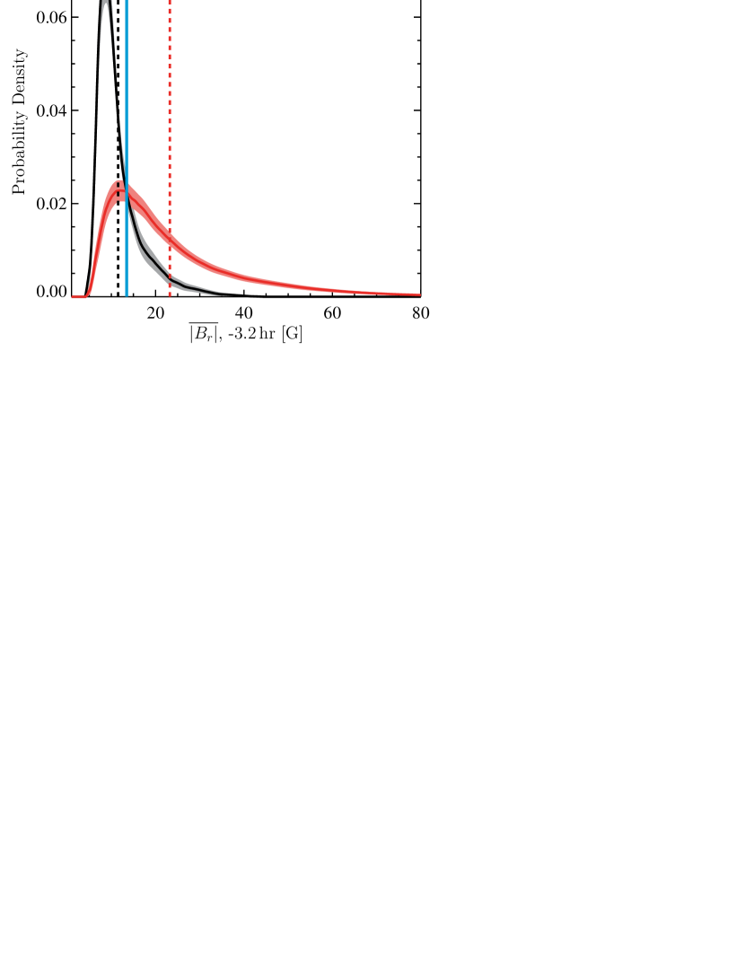
Figure 1.— Nonparametric discriminant analysis for the mean unsigned magnetic flux, $\overline{|B_{r}|}$. Left: probability density estimates for the NE regions (black), and the PE regions (red) in time interval 4, centered 3.2 hr before the emergence time, with the mean of each sample indicated by a vertical dashed line in the corresponding color. The shaded region is a 1-$\sigma$ estimate of the uncertainty. The discriminant boundary, where the two probability density estimates are equal, is indicated by a vertical blue line; an observation to the right of the boundary would be classified as an emergence. There is an obvious difference between the density estimates for the NE and PE regions: the PE distribution has a longer tail to high field strength, but there is also considerable overlap of the distributions. Right: evolution of the Peirce skill score. There is perhaps a weak increase in the performance of $\overline{|B_{r}|}$ closer to the emergence time that is likely due to the onset of emergence during time interval 4 for some regions, but for most of the time intervals shown, the skill score is approximately constant.

The right panel of Figure 1 shows the performance of $\overline{|B_{r}|}$ as a function of time prior to emergence. There is perhaps an increase in the skill score from approximately one day before emergence to a few hours before emergence, but the overall increase is not large in magnitude. Certainly between 24.5 hr and 8.5 hr before emergence, the variations in the skill score are less than the uncertainty; there is a small increase in the last point, 3.2 hr prior to emergence, which is likely to be a result of an incorrect emergence time for some regions, so that surface field is appearing during the final time interval (c.f. Fig. 11 of Paper I).

This constancy in the performance of the unsigned field is largely because the field itself does not evolve substantially over the time in question. Figure 2 (left) shows the field 24.5 hr before emergence versus the field 8.5 hr before emergence. There is an extremely high correlation between the field at the two times (Pearson correlation coefficients $\geq 0.96$) for both the PE and NE regions, and no clear indication of evolution. When considering the change between 24.5 hr and 3.2 hr before emergence (Fig. 2, right), there is some indication of evolution of the field, consistent with there being a few regions for which emergence began in the final six hours before the nominal emergence time (more points lying above and to the left of the blue line). This trend is still weak compared to the variation among the regions considered, as is born out by the small decrease in the correlations (Pearson correlation coefficients $\geq 0.94$). Thus the evolution of the field does not greatly change the ability of the unsigned field to distinguish the PE from the NE.

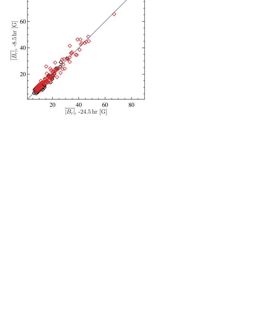
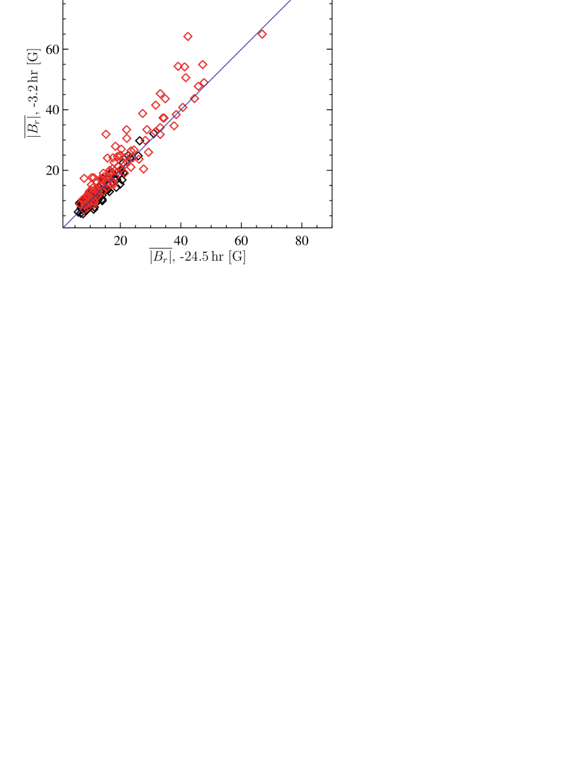
Figure 2.— Left: scatter plot of $\overline{|B_{r}|}$ for the time interval centered 24.5 hr emergence versus the time interval centered 8.5 hr before emergence for NE (black) and PE (red) regions. The Pearson correlation coefficient between the PE at these times is $0.98\pm 0.01$, while for the NE it is $0.96\pm 0.01$. Right: same scatter plot but between 24.5 hr and 3.2 hr before emergence. The correlation coefficients are both slightly lower at $0.95\pm 0.01$ for PE and $0.94\pm 0.01$ for NE, suggesting that much of the evolution of the flux occurs between 8.5 hr and 3.2 hr before emergence, which is consistent with the emergence process beginning (for some regions) during the final six hours before the time of emergence.

The large overlap between the distributions of NE and PE regions shows that there is no clear signature in the surface field when individual regions are considered (c.f. Fig. 2 and 3 of Paper II). However, there was a bias introduced in the selection criteria for the NE compared with the PE: NE regions were required to have magnetic field consistently $<1000$ G (see §3.2 of Paper I), while no such requirement was imposed for PE regions. It may simply be that the difference between the PE and NE samples results from the bias in the selection of NE compared to the PE regions.

It is also possible that there is a small amount of weak magnetic flux present at the surface more than a day prior to the beginning of the clear emergence phase of active regions. This field is indistinguishable from noise in individual MDI magnetograms, but becomes apparent in averaging over large numbers. This could be related to the emergence process, in the form of small amounts of flux arriving at the emergence site prior to the main emergence, as is seen in some simulations (e.g., Cheung et al., 2010; Stein et al., 2011). It could also be related to the known tendency for active regions to emerge in the same locations as prior active regions (e.g., Pojoga & Cudnik, 2002). The latter case would be one example of how the bias manifests from a completely solar cause.

4.2. Measures of the Center-to-Annulus and Annulus-to-Center Travel Times

Immediately prior to emergence, the mean travel-time shift measured in a variety of filters shows a significant ability to distinguish PE from NE regions. The left panel of Figure 3 shows the mean travel-time, $\overline{\delta\tau_{\rm mn}}$, in filter TD5, for time interval 4 (centered 3.2 hr prior to the time of emergence). The NE sample has a mean very close to 0 s, and its distribution is symmetric and peaked close to 0 s, consistent with the differences from 0 s being simply due to noise. The mean of the PE sample is negative and close to the peak in its distribution; the PE distribution is slightly wider than the NE distribution. Although there is a distinct difference visible in the distributions, there is also substantial overlap between the two, as in the $\overline{|B_{r}|}$ case. This is quantified by a Peirce skill score of $0.45\pm 0.08$. Regions with a mean travel-time shift less than the discriminant boundary (at approximately -0.2 s) would be classified as PE, while those above would be classified as NE. That is, negative mean travel-time shifts are associated with emerging regions. Like the average unsigned field, the performance of the mean travel-time shift is better 3.2 hr before emergence than at earlier times (compare Fig. 1, right to Fig. 3, right).

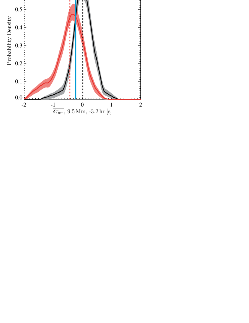
Figure 3.— Nonparametric discriminant analysis for the mean travel-time shift, $\overline{\delta\tau_{\rm mn}}$, in filter TD5, in the same format as Fig. 1. Left: there is an obvious difference between the density estimates for the NE and PE regions in the time interval centered 3.2 hr before the emergence time, with the PE regions typically having negative mean travel-time shifts. Right: the performance of $\overline{\delta\tau_{\rm mn}}$ shows a similar trend to $\overline{|B_{r}|}$, constant for most of the time considered, with an increase at the last time interval, although the skill score is consistently lower for $\overline{\delta\tau_{\rm mn}}$.

The mean travel-time shift is typically reduced in the presence of surface magnetic field (e.g., Lindsey & Braun, 2005; Braun & Birch, 2008). Figure 4 shows the Pearson correlation coefficient between $\overline{\delta\tau_{\rm mn}}$ and $\overline{|B_{r}|}$ as a function of time. The correlation coefficient for the NE regions is generally close to 0, as would be expected if the mean travel-time shifts are simply due to noise, while for the PE regions, the correlation coefficient is negative, with perhaps a weak trend towards a stronger (negative) correlation closer to the emergence time, although there is not a distinct difference between the final time interval prior to emergence and earlier time intervals. It is possible that the difference between the PE and NE regions in $\overline{\delta\tau_{\rm mn}}$ is simply an indirect result of the difference in the surface field. However, it is also possible that there is a signal in $\overline{\delta\tau_{\rm mn}}$ during all the time intervals that is not a result of the surface magnetic field. The influence of the surface field on the travel-times is investigated further in §4.5.

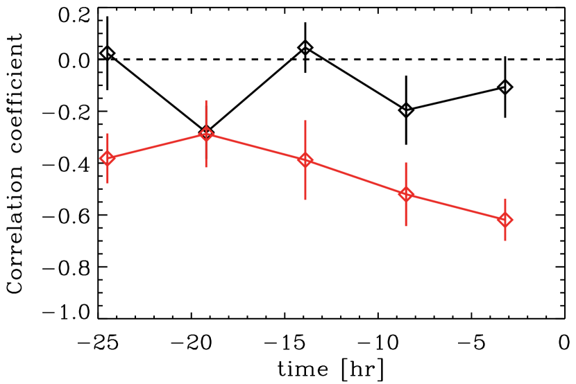
Figure 4.— Pearson correlation coefficient between $\overline{|B_{r}|}$ and $\overline{\delta\tau_{\rm mn}}$ in filter TD5 from a bootstrap method for the NE (black) and PE (red) regions as a function of time. For the NE regions, the correlation coefficient is generally close to zero, as expected. For the PE regions, there is a weak trend towards stronger (negative) correlations at later times.

There are also many instances where $\overline{\delta\tau_{\rm in}}$ and $\overline{\delta\tau_{\rm out}}$ have a skill score only slightly less than $\overline{\delta\tau_{\rm mn}}$ in the same filter. In all time intervals and filters, there is a moderate correlation between $\overline{\delta\tau_{\rm in}}$ and $\overline{\delta\tau_{\rm out}}$. Since $\overline{\delta\tau_{\rm mn}}$ is a linear combination of $\overline{\delta\tau_{\rm in}}$ and $\overline{\delta\tau_{\rm out}}$, it is likely that the slightly better performance of $\overline{\delta\tau_{\rm mn}}$ is simply a result of a better signal to noise ratio than either $\overline{\delta\tau_{\rm in}}$ or $\overline{\delta\tau_{\rm out}}$ considered alone.

4.3. East-West and North-South Travel Times

In Table 4, antisymmetric averages of the east-west and north-south travel-time differences appear most frequently at shallow to moderate depths and earlier time intervals. The left panels of Figure 5 show the distributions of $\overline{\delta\tau_{x}\cos\theta}$ and $\overline{\delta\tau_{y}\sin\theta}$ in filter TD3, centered 24.5 hr before emergence. For both variables, the mean and the peak of the NE distributions lie close to 0 s, while the mean and the peak of the PE distributions are at positive travel-time differences of approximately 1 s. Unlike previous variables considered, there are multiple discriminant boundaries; the boundaries in the tails of the distributions, at large negative values of $\overline{\delta\tau_{x}\cos\theta}$ and large positive values of $\overline{\delta\tau_{y}\sin\theta}$, are likely to be spurious results caused by a few regions having extreme values.

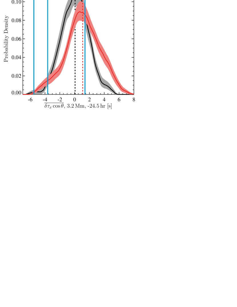
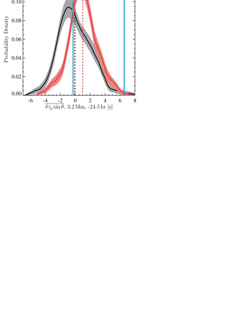
Figure 5.— Nonparametric discriminant analysis for antisymmetric averages of the east-west and north-south travel-time differences, $\overline{\delta\tau_{x}\cos\theta}$ (top) and $\overline{\delta\tau_{y}\sin\theta}$ (bottom) in filter TD3, in the same format as Fig. 1. Left: the density estimates for NE regions for both $\overline{\delta\tau_{x}\cos\theta}$ and $\overline{\delta\tau_{y}\sin\theta}$, 24.5 hr before the emergence time, are peaked close to 0 s, and are fairly symmetric; the density estimates for PE regions are both peaked close to 1 s. Right: given the uncertainties, there is no obvious trend in $\overline{\delta\tau_{x}\cos\theta}$ and only weak evidence for a trend towards worse performance closer to emergence for $\overline{\delta\tau_{y}\sin\theta}$.

The evolution of the skill score (Fig. 5, right) shows that the variations with time are unlikely to be real given the uncertainties in the resulting skill scores, although there is perhaps a trend for worse performance of $\overline{\delta\tau_{y}\sin\theta}$ at times closer to the emergence time. However, this is one example of a variable that, in one time interval, falls above the threshold to be included in Table 4, while in other time intervals, it may be excluded from the table, despite have substantial ability to discriminate PE from NE regions.

The particular combinations that appear, namely $\overline{\delta\tau_{x}\cos\theta}$ and $\overline{\delta\tau_{y}\sin\theta}$, would be expected to have a signal from a converging flow. However, note that only one instance of $\overline{\delta\tau_{\rm oi}}$ appears in this table, and in a filter with a much deeper lower turning point. The relative strength of the signals in $\overline{\delta\tau_{x}\cos\theta}$ and $\overline{\delta\tau_{y}\sin\theta}$ versus the signal in $\overline{\delta\tau_{\rm oi}}$ in general depends on the geometry of the assumed flow; detailed modeling is beyond the scope of the current work. We note, however, that Figure 5 of Paper II shows patterns in the ensemble averages of $\overline{\delta\tau_{x}\cos\theta}$ and $\overline{\delta\tau_{y}\sin\theta}$ with more structure than would be expected for a simple converging flow. As discussed in Paper II, one potential interpretation for the signals in $\overline{\delta\tau_{x}\cos\theta}$ and $\overline{\delta\tau_{y}\sin\theta}$ is a preference for emergence to occur at the boundary between supergranules, so these signals are the result of supergranular flows, not the emergence process itself.

4.4. The Vorticity

The remaining variable appearing multiple times in the list of best parameters is $\overline{\rm vor\sin\theta}$, particularly in filter TD4. Figure 6 (left) shows a small but clear offset in the distributions of the NE and PE regions 24.5 hr before the emergence time, with PE regions more likely to have negative values of $\overline{\rm vor\sin\theta}$ relative to NE regions. As for the variables $\overline{\delta\tau_{x}\cos\theta}$ and $\overline{\delta\tau_{y}\sin\theta}$, this is an example of a variable that, in some time intervals, falls above the threshold to be included in Table 4, while in other time intervals, it is excluded from the table, despite have substantial ability to discriminate PE from NE regions (see Fig. 6, right).

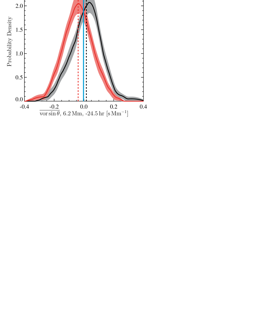
Figure 6.— Nonparametric discriminant analysis for an antisymmetric average of the vertical vorticity, $\overline{\rm vor\sin\theta}$, in filter TD4, in the same format as Fig. 1. Left: 24.5 hr before the emergence time, the density estimate for NE regions has a peak at and a mean value that are slightly positive, while the peak and mean value for the PE distribution are at negative values. Right: given the uncertainties in the skill score, the performance of this variable does not clearly evolve with time.

It is known that surface magnetic fields are associated with a prograde flow (e.g., Zhao et al., 2004). Such a prograde flow would result in the signal seen in $\overline{\rm vor\sin\theta}$, so one explanation for this is that, once again, the difference between the PE and NE regions is a result of the surface magnetic field. To determine whether there is a helioseismic signature of the emergence process not caused by the surface magnetic field, it is important to account for the contribution of the surface field to the differences in the travel-times.

4.5. Matching the Flux Distribution

To investigate the influence of the surface magnetic field on the helioseismic parameters, we selected subsets of the NE and PE regions with matching distributions of average unsigned field, $\overline{|B_{r}|}$, and location on the disk. The approach to this was essentially the same as the selection of the NE regions to match the distributions in position and time of the PE regions described in Paper I: we used simulated annealing to select subsets of PE and NE regions that minimize the integrated absolute value of the difference between nonparametric density estimates for the two distributions. Sixty-five regions from each sample were selected, which resulted in 50–55 regions with good duty cycle in each sample. This was the largest subset for which an integrated absolute difference of no more than about 0.1 could be obtained; the integrated absolute difference of two completely non-overlapping distributions would be 2.

We performed the same analysis as for the full set of regions on these subsets of regions to rank the variables by skill score. We also repeated the Monte Carlo experiment (see appendix B) for these sample sizes. We found that although the maximum skill scores of the helioseismology variables can reasonably be expected when there is no difference in the populations, there is still a preponderance of large skill score values in the helioseismology variables compared to what would be expected from chance. This suggests that some of the helioseismology variables have real ability to discriminate the PE regions from the NE regions, but that it is difficult to determine if any specific variable has any power to discriminate. Because of this, we choose to show variables with Peirce skill scores greater than 0.24 (rather than the 0.27 used for the full samples) in Table 5. This is done to highlight the variables (shaded in the table) that still have large skill scores after the flux matching.

Table 5Best Performing Variables

variable	depth	Peirce SS
	(Mm)
TI-0: time=$t_{0}-24.5$ hr
$\overline{\delta\tau_{y}\sin\theta}^{\dagger}$	3.2	$0.33\pm 0.10$
$\overline{\delta\tau_{y}\sin\theta}^{\dagger}$	2.2	$0.32\pm 0.11$
$\overline{\rm vor\sin\theta}^{\dagger}$	15.7	$0.31\pm 0.12$
$\overline{\delta\tau_{x}}$	20.9	$0.29\pm 0.10$
$\overline{\rm div}$	9.5	$0.27\pm 0.10$
$\overline{\rm vor\sin\theta}^{\dagger}$	6.2	$0.27\pm 0.11$
$\overline{\delta\tau_{x}\cos\theta}$	6.2	$0.24\pm 0.11$
$\overline{\delta\tau_{\rm io}\cos\theta}$	3.2	$0.24\pm 0.11$
TI-1: time=$t_{0}-19.2$ hr
$\overline{\delta\tau_{\rm out}\cos\theta}$	9.5	$0.25\pm 0.10$
$\overline{\rm div\sin\theta}$	15.7	$0.25\pm 0.12$
$\overline{\delta\tau_{\rm in}\cos\theta}$	6.2	$0.25\pm 0.11$
$\overline{\rm vor\sin\theta}$	11.4	$0.25\pm 0.11$
$\overline{\delta\tau_{x}}$	2.2	$0.24\pm 0.11$
$\overline{\delta\tau_{x}\cos\theta}$	9.5	$0.24\pm 0.12$
$\overline{\delta\tau_{\rm in}\cos\theta}$	15.7	$0.24\pm 0.11$
$\overline{\delta\tau_{\rm io}\cos\theta}$	9.5	$0.24\pm 0.10$
$\overline{\delta\tau_{\rm out}}$	3.2	$0.24\pm 0.12$
$\overline{\delta\tau_{x}}$	3.2	$0.24\pm 0.11$
TI-2: time=$t_{0}-13.9$ hr
$\overline{\rm div\cos\theta}$	15.7	$0.36\pm 0.10$
$\overline{\rm vor}$	23.3	$0.30\pm 0.10$
$\overline{\rm vor\sin\theta}^{\dagger}$	6.2	$0.29\pm 0.11$
$\overline{\delta\tau_{x}\cos\theta}$	9.5	$0.26\pm 0.11$
$\overline{\rm div}$	6.2	$0.26\pm 0.11$
$\overline{\delta\tau_{x}\cos\theta}^{\dagger}$	3.2	$0.25\pm 0.12$
$\overline{\delta\tau_{x}}$	15.7	$0.25\pm 0.13$
$\overline{\rm div}$	13.3	$0.24\pm 0.11$
$\overline{\delta\tau_{y}\cos\theta}$	11.4	$0.24\pm 0.12$
$\overline{\delta\tau_{x}\cos\theta}$	15.7	$0.24\pm 0.12$
TI-3: time= $t_{0}-8.5$ hr
$\overline{\rm div}$	11.4	$0.36\pm 0.11$
$\overline{\delta\tau_{x}\cos\theta}$	2.2	$0.26\pm 0.12$
$\overline{\rm vor\cos\theta}$	6.2	$0.25\pm 0.11$
$\overline{\delta\tau_{x}\cos\theta}$	6.2	$0.25\pm 0.12$
$\overline{\delta\tau_{\rm io}\cos\theta}$	1.4	$0.25\pm 0.12$
$\overline{\delta\tau_{x}\cos\theta}$	3.2	$0.25\pm 0.13$
TI-4: time= $t_{0}-3.2$ hr
$\overline{\delta\tau_{\rm mn}}^{\dagger}$	9.5	$0.38\pm 0.09$
$\overline{\rm vor\sin\theta}^{\dagger}$	6.2	$0.33\pm 0.11$
$\overline{\delta\tau_{\rm out}}^{\dagger}$	9.5	$0.30\pm 0.10$
$\overline{\delta\tau_{x}}$	6.2	$0.29\pm 0.11$
$\overline{\delta\tau_{\rm out}\cos\theta}$	13.3	$0.29\pm 0.12$
$\overline{\delta\tau_{\rm in}}^{\dagger}$	9.5	$0.28\pm 0.12$
$\overline{\delta\tau_{\rm mn}}^{\dagger}$	23.3	$0.28\pm 0.12$
$\overline{\rm vor}$	2.2	$0.28\pm 0.11$
$\overline{\delta\tau_{\rm out}\cos\theta}$	9.5	$0.27\pm 0.11$
$\overline{\rm vor\cos\theta}$	23.3	$0.26\pm 0.11$
$\overline{\delta\tau_{\rm io}\cos\theta}$	20.9	$0.25\pm 0.11$
$\overline{\delta\tau_{\rm out}\cos\theta}$	11.4	$0.24\pm 0.11$
$\overline{\delta\tau_{\rm mn}}^{\dagger}$	20.9	$0.24\pm 0.11$
$\overline{\delta\tau_{x}}$	3.2	$0.24\pm 0.13$
$\overline{\delta\tau_{\rm mn}}$	18.2	$0.24\pm 0.10$
$\overline{\delta\tau_{x}\cos\theta}^{\dagger}$	3.2	$0.24\pm 0.12$
$\overline{\delta\tau_{y}\sin\theta}^{\dagger}$	2.2	$0.24\pm 0.13$

Note. — Depth refers to the lower turning point of the waves in the filter used. Time is relative to the emergence time $t_{0}$. Variables marked with a ^† also appear in Table 4. A version of Table 5 containing all the variables considered is published in the electronic edition of Barnes et al. (2013).

Due to the matching of the distributions, $\overline{|B_{r}|}$ has virtually no ability to discriminate between the samples, and thus does not appear anywhere in Table 5. To illustrate how well the distributions match, the distributions of $\overline{|B_{r}|}$ in time interval 0, a day before emergence, are shown in Figure 7, along with the skill score as a function of time. The skill score is consistent with zero in time intervals 0–3, and compared with Figure 1, the PE and NE distributions are very closely matched, with no remaining tail to large values of $\overline{|B_{r}|}$ for the PE sample. The increase in skill score in time interval 4 is likely due to the start of emergence in a few regions.

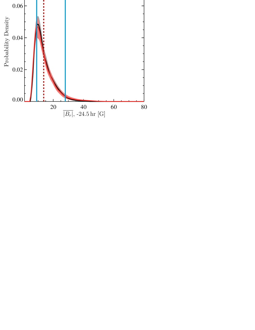
Figure 7.— Nonparametric discriminant analysis for the mean unsigned magnetic flux, $\overline{|B_{r}|}$, for a subset of regions with matched distributions of magnetic flux, in the same format as Fig. 1. By construction of the subset, the distributions of PE and NE regions are closely matched, as seen in the left panel, thus the Peirce skill score is consistent with 0 for time intervals 0–3, as it should be for matched distributions, with a slight increase at the final time interval likely due to the onset of emergence during time interval 4 for some regions.

For most of the variables that are not strongly correlated with the magnetic flux, the skill score values have not changed substantially, but the smaller sample sizes generally lead to larger uncertainties. Almost every filter and depth combination of $\overline{\delta\tau_{x}\cos\theta}$, $\overline{\delta\tau_{y}\sin\theta}$ and $\overline{\rm vor\sin\theta}$ present in Table 4 is also present after flux matching in Table 5, with a similar value of the skill score. For example, in time interval 0, the skill score values $\overline{\delta\tau_{y}\sin\theta}$ and $\overline{\rm vor\sin\theta}$ for the filters found in Table 4 lie in the range $0.27\leq{\rm PSS}\leq 0.34$ for both the full samples and the matched flux subsets. By contrast, the mean travel-time shifts in time interval 4 have consistently lower skill scores for the matched flux subset, indicating that the correlation with the magnetic flux accounts for some of the ability of $\overline{\delta\tau_{\rm mn}}$ (and $\overline{\delta\tau_{\rm in}}$ and $\overline{\delta\tau_{\rm out}}$) to discriminate between PE and NE regions. In addition to the best performing variables for the full samples of PE and NE regions, there are a considerable number of other variables, in a range of filters, present in Table 5. Many of these are likely to be statistical anomalies, with no real ability to discriminate the PE and NE regions.

Figure 8 shows the probability density estimates and the time variation of the skill score for $\overline{\delta\tau_{y}\sin\theta}$ in filter TD3 and for $\overline{\rm vor\sin\theta}$ in filter TD4. Qualitatively, the results are extremely similar to those shown in Figures 5, bottom and 6, where the full sets of regions were included. The distributions are peaked at similar values, with similar widths, leading to discriminant boundaries in approximately the same locations. The main difference is that the uncertainty in the skill score has increased slightly. Thus, the ability of these variables to distinguish PE from NE regions is not a result of a difference in the average unsigned vertical field between the two samples, although it could still be a result of a different aspect of the surface field (e.g., the horizontal field, or small areas of strong vertical field).

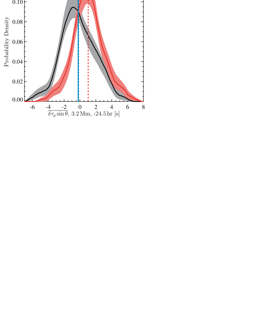
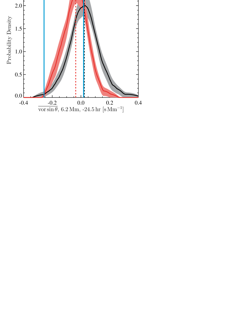
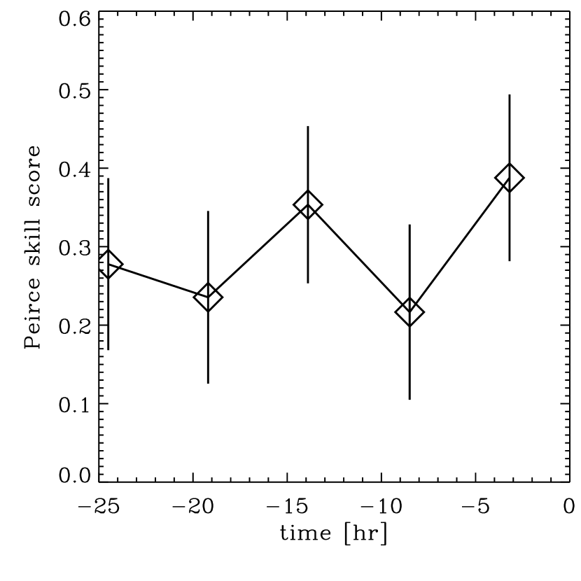
Figure 8.— Nonparametric discriminant analysis for antisymmetric averages of the north-south travel-time differences, $\overline{\delta\tau_{y}\sin\theta}$, in filter TD3 (top), and for the vertical vorticity, $\overline{\rm vor\sin\theta}$, in filter TD4 (bottom), for a subset of regions with matched distributions of average magnetic flux, in the same format as Fig. 1. The results are qualitatively very similar to those seen in Fig. 5 (bottom) and 6 for the full samples. The largest change is an increase in the uncertainties caused by the smaller sample sizes.

5. Discussion

There are statistically significant differences between the properties of the pre-emergence and non-emergence samples that persist, with relatively little change, for at least a day prior to the onset of emergence. However, these differences are small, of order 1 s or less in the travel-time shifts on average, thus none of the variables considered can clearly distinguish an emergence from a non-emergence for any single region (c.f. Figs. 2 and 3 from Paper II). This is quite different from the results of Ilonidis et al. (2011), who found much larger travel-time reductions, although that study considered waves that propagate much deeper than were considered here.

The average unsigned magnetic flux at the surface was the best discriminator between the two samples. This could be a result of the appearance of small amounts of flux at the surface, starting at least one day prior to our definition of emergence time. The MDI instrument is unable to resolve this flux in a single magnetogram, and thus it is only distinguishable when averaging over many regions. Simulations of flux emergence (e.g., Cheung et al., 2010; Stein et al., 2011) do exhibit this type of behavior, thus our investigation shows some support for these simulations.

It is also possible that the ability of the average magnetic flux to distinguish the two samples is a result of a bias in the samples, either of solar origin, or as a result of our selection criteria. Our selection of NE regions (see Paper I) imposed a maximum field strength allowed that was not similarly applied to the PE regions. This could have resulted in a bias between the two samples in the average flux. However, it is also possible that the difference in average flux is a result of the tendency for active regions to emerge in the same location as prior active regions (e.g., Pojoga & Cudnik, 2002), and not directly related to the emergence process.

While such considerations are important if the goal is to use helioseismology to predict the emergence of active regions, our goal is simply to determine if there is a helioseismic signal of emergence. The helioseismic measures that best distinguish the pre-emergence from the non-emergence regions are mean travel-time shifts, particularly immediately prior to emergence, antisymmetric averages of north-south and east-west travel-time differences, and an antisymmetric average of the vertical vorticity. The mean travel-time shifts are correlated with the presence of surface field, and thus may not be related to subsurface properties of the emergence. This was confirmed by the reduced ability of mean travel-time shifts to distinguish PE from NE regions for subsets of the initial samples of PE and NE regions that had matched distributions of average unsigned magnetic flux.

The signals in the north-south and east-west travel-time differences, and the signal in the vertical vorticity appear to not be sensitive to the surface field. Thus, we believe there are differences in the subsurface flows that can be detected by helioseismology prior to the emergence of significant magnetic flux. A converging flow could qualitatively explain the signals seen in the north-south and east-west travel-time differences, but it appears that the flow pattern is not a simple converging flow. A prograde flow below the site of the emergence would produce the observed pattern in the vertical vorticity. This is perhaps related to the “small shearing flow feature” at a depth of 2 Mm described by Kosovichev & Duvall (2008) for AR 10488. There is no clear evidence for a retrograde flow, as would be expected from typical rising flux tube simulations (e.g., Fan, 2008), although these simulations end approximately 20 Mm below the surface. Instead, we found the vertical vorticity to be consistent with a prograde flow, and the difference in north-south travel-time differences is comparable to that in east-west travel-time differences, as would result from a converging flow. Thus our results suggest that the properties of simulated rising flux tubes must change as they approach the surface, at shallower depths than are presently simulated, if this is the mechanism by which active regions form.

As noted in Paper I, there are several ways in which a future investigation could improve on the present method. However, we have already found subtle but significant differences in the helioseismic signals from our samples of pre-emergence and non-emergence regions that suggest a detectable subsurface manifestation of active region formation prior to the appearance of significant surface magnetic flux. Our statistical results place strong constraints on models of active region formation.

Appendix A The Influence of Duty Cycle

Because of the varying duty cycle, some regions are only present in a subset of the time intervals. This could potentially influence the results, if there is a handful of regions (with varying duty cycle) that are easy to classify. To check this, the analysis was repeated for the subset of regions that had a good duty cycle for every time interval. This severely reduces the sample sizes, to 48 and 45 for PE and NE respectively. The main impact of this is an increase in the error bars, which is expected from the reduction in the sample sizes, without greatly changing the results. To illustrate this, the right panels of Figures 1, 3, and 5 have been reproduced in Figure 9 with this subset. All the other plots exhibit the same behavior, thus we believe that this does not affect any of our conclusions.

Figure 9.— Evolution of the Peirce skill score for four variables: top, left: $\overline{|B_{r}|}$, top, right: $\overline{\delta\tau_{\rm mn}}$ in filter TD5, bottom, left: $\overline{\delta\tau_{x}\cos\theta}$ in filter TD3, and bottom, right: $\overline{\delta\tau_{y}\sin\theta}$ in filter TD3. Only regions with good data for all time intervals and seismology variables were used. Compared to the right panels of Figs. 1, 3, 5, in which all available regions were used in each plot, the same trends (or lack of trends) are seen, but with larger uncertainties.

Appendix B Monte-Carlo Experiment

Given the number of variables considered compared to the number of data points, one should ask the question: are these results simply a statistical fluke? To answer this, a Monte Carlo experiment was performed. To represent one variable, two random samples of 85 points (typical of the sample sizes in §4 and Table 4) each were drawn from the same normal distribution. This was repeated for 66,250 variables (50 times the number of active region emergence variables), changing only the random number seed between variables. Nonparametric discriminant analysis was applied to the resulting values, and an unbiased bootstrap estimate of the Peirce skill score was made for each variable. The distribution of the resulting skill scores is shown in Figure 10, left, along with the distribution of the variables considered for active region emergence. Compared with the random variables, there is a preponderance of large skill score values for the emergence variables. Dividing the random variables into 50 sets of size equal to the number of emergence variables shows that the typical maximum skill score achieved is about 0.27, so the probability of getting a skill score greater than that if there is no information in the variable is extremely small. However, the distribution of random variables and of active region emergence variables show considerable overlap below a skill score of about 0.2.

Figure 10.— Probability density of Peirce skill scores from the Monte Carlo experiment (dashed curve) with $1-\sigma$ error estimate (dotted curves) and from the variables considered for active region emergence (solid curve), using a bootstrap estimate. The left panel shows the results for sample sizes of 85; the right panel shows the results for sample sizes of 50. There is a clear tail of the distribution of the active region emergence variables to larger skill scores not present for the random variables, indicating that it is very unlikely that chance alone accounts for the performance of the best variables at distinguishing PE from NE regions. For the sample size of 85, the variables with skill scores above 0.27 almost certainly have a real ability to discriminate between PE and NE regions; for the sample size of 50, it is difficult to determine if any specific helioseismology variable has a real ability to discriminate between PE and NE regions, but the number of helioseismology variables with large skill scores ($\gtrsim 0.2$) suggests that some can discriminate between the two.

To compare with the results when the distribution of magnetic flux was matched between NE and PE regions (§4.5 and Table 5), the experiment was repeated for two random samples of 50 points each. The resulting distribution of skill scores is shown in Figure 10, right. There is still a preponderance of large skill scores for the emergence variables compared to the random variables, but it is less pronounced than for the larger sample size. Again dividing the random variables into 50 sets of size equal to the number of emergence variables shows that the typical maximum skill score achieved is now about 0.34, but was as high as 0.43. In this case, it is no longer possible to determine whether any individual variable has any real ability to discriminate between PE and NE regions. However, it is possible to infer that there are more variables with high skill scores than would be expected from chance alone. The number of variables with skill score $\geq 0.27$ (the value used in Table 4) is 17, compared with an expected number of 11. The chance of getting at least this many variables by chance is approximately 2%. The number of variables with skill score $\geq 0.2$ is 120, compared with an expected number of 86. The chance of getting at least this many variables by chance is less than 2%. Thus there is reason to believe that there is a difference in the helioseismology variables between PE and NE regions.

For the results presented here, the distributions were assumed to be normal, as this is a reasonable approximation to the expected noise distribution. However, to confirm the results, the Monte Carlo experiments were also performed drawing at random from a Cauchy distribution and from a cosine distribution. For the Cauchy distribution, which has longer tails than a normal distribution, the largest skill scores obtained were less than the largest skill scores for the normal distribution. For the cosine distribution, which has shorter tails than a normal distribution, the largest skill scores were very similar to those obtained from the normal distribution. In all cases, there is a clear tail of the distribution of the emergence variables to larger skill scores not present for the random variables, indicating that it is very unlikely that chance alone accounts for the performance of the best variables at distinguishing PE from NE regions.

References

- Birch et al. (2013) Birch, A. C., Braun, D. C., Leka, K. D., Barnes, G., & Javornik, B. 2013, ApJ, 762, 131
- Brandenburg (2005) Brandenburg, A. 2005, ApJ, 625, 539
- Braun (1995) Braun, D. C. 1995, in Astronomical Society of the Pacific Conference Series, Vol. 76, GONG 1994. Helio- and Astro-Seismology from the Earth and Space, ed. R. K. Ulrich, E. J. Rhodes Jr., & W. Dappen, 250
- Braun & Birch (2008) Braun, D. C. & Birch, A. C. 2008, Sol. Phys., 251, 267
- Chang et al. (1999) Chang, H., Chou, D., & Sun, M. 1999, ApJ, 526, L53
- Cheung et al. (2010) Cheung, M. C. M., Rempel, M., Title, A. M., & Schüssler, M. 2010, ApJ, 720, 233
- Couvidat et al. (2005) Couvidat, S., Gizon, L., Birch, A. C., Larsen, R. M., & Kosovichev, A. G. 2005, ApJS, 158, 217
- Duvall et al. (1993) Duvall, Jr., T. L., Jefferies, S. M., Harvey, J. W., & Pomerantz, M. A. 1993, Nature, 362, 430
- Efron & Gong (1983) Efron, B. & Gong, G. 1983, Am. Statist., 37, 36
- Fan (2008) Fan, Y. 2008, ApJ, 676, 680
- Fan (2009) —. 2009, Living Reviews in Solar Physics, 6, 4
- Gizon & Birch (2005) Gizon, L. & Birch, A. C. 2005, Living Reviews in Solar Physics, 2, 6
- Gizon et al. (2010) Gizon, L., Birch, A. C., & Spruit, H. C. 2010, ARA&A, 48, 289
- Hartlep et al. (2011) Hartlep, T., Kosovichev, A. G., Zhao, J., & Mansour, N. N. 2011, Sol. Phys., 268, 321
- Harvey et al. (1998) Harvey, J., Tucker, R., & Britanik, L. 1998, in ESA Special Publication, Vol. 418, Structure and Dynamics of the Interior of the Sun and Sun-like Stars, ed. S. Korzennik, 209
- Hill et al. (2003) Hill, F., Bolding, J., Toner, C., Corbard, T., Wampler, S., Goodrich, B., Goodrich, J., Eliason, P., & Hanna, K. D. 2003, in ESA Special Publication, Vol. 517, GONG+ 2002. Local and Global Helioseismology: the Present and Future, ed. H. Sawaya-Lacoste, 295–298
- Hills (1966) Hills, M. 1966, J. R. Statist. Soc. B, 28, 1
- Ilonidis et al. (2011) Ilonidis, S., Zhao, J., & Kosovichev, A. 2011, Sci, 333, 993
- Jensen et al. (2001) Jensen, J. M., Duvall, Jr., T. L., Jacobsen, B. H., & Christensen-Dalsgaard, J. 2001, ApJ, 553, L193
- Kendall et al. (1983) Kendall, M., Stuart, A., & Ord, J. K. 1983, The Advanced Theory of Statistics, 4th edn., Vol. 3 (New York: Macmillan Publishing Co., Inc)
- Komm et al. (2009) Komm, R., Howe, R., & Hill, F. 2009, Sol. Phys., 258, 13
- Komm et al. (2011) —. 2011, Sol. Phys., 268, 407
- Kosovichev (2009) Kosovichev, A. G. 2009, Space Sci. Rev., 144, 175
- Kosovichev & Duvall (2008) Kosovichev, A. G. & Duvall, Jr., T. L. 2008, in Astronomical Society of the Pacific Conference Series, Vol. 383, Subsurface and Atmospheric Influences on Solar Activity, ed. R. Howe, R. W. Komm, K. S. Balasubramaniam, & G. J. D. Petrie, 59–70
- Leka et al. (2013) Leka, K. D., Barnes, G., Birch, A. C., Gonzalez-Hernandez, I., Dunn, T., Javornik, B., & Braun, D. C. 2013, ApJ, 762, 130
- Lindsey & Braun (2000) Lindsey, C. & Braun, D. C. 2000, Sol. Phys., 192, 261
- Lindsey & Braun (2005) —. 2005, ApJ, 620, 1107
- Peirce (1884) Peirce, C. S. 1884, Sci, 4, 453
- Pojoga & Cudnik (2002) Pojoga, S. & Cudnik, B. 2002, Sol. Phys., 208, 17
- Silverman (1986) Silverman, B. W. 1986, Density Estimation for Statistics and Data Analysis (London: Chapman and Hall)
- Stein et al. (2011) Stein, R. F., Lagerfjärd, A., Nordlund, Å., & Georgobiani, D. 2011, Sol. Phys., 268, 271
- Woodcock (1976) Woodcock, F. 1976, Monthly Weather Review, 104, 1209
- Zhao et al. (2004) Zhao, J., Kosovichev, A. G., & Duvall, Jr., T. L. 2004, ApJ, 607, L135
- Zharkov & Thompson (2008) Zharkov, S. & Thompson, M. J. 2008, Sol. Phys., 251, 369