The Changing Geometry of a Fitness Landscape Along an Adaptive Walk

Abstract.

It has recently been noted that the relative prevalence of the various kinds of epistasis varies along an adaptive walk. This has been explained as a result of mean regression in NK model fitness landscapes. Here we show that this phenomenon occurs quite generally in fitness landscapes. We propose a simple and general explanation for this phenomenon, confirming the role of mean regression. We provide support for this explanation with simulations, and discuss the empirical relevance of our findings.

Corresponding author: Kristina Crona, kcrona@ucmerced.edu

Author Summary

The main result concerns the changing geometry along an adaptive walk in a fitness landscape. An adaptive walk is described by a sequence of genotypes of increasing fitness, where two consecutive genotypes differ by a point mutation. We compare patterns of epistasis, or gene interactions, along adaptive walks. Roughly, epistasis is antagonistic (rather than synergistic) if the double mutant combining two beneficial mutations has lower fitness than expected. In the extreme case that the double mutant has lower fitness than one (or both) of the single mutants, one has sign epistasis. We claim that the further one is along an adaptive walk, the larger the frequency of sign epistasis and the smaller the relative amount of antagonistic epistasis relative to synergistic epistasis. We provide a simple and general argument for our claim, which hence likely applies to empirical fitness landscapes. Our claims can readily be checked by empirical biologists. Potential theoretical progress related to our work includes a better understanding of the role of recombination in evolution.

introduction

Darwinian evolution can be illustrated as an uphill or adaptive walk in a multidimensional landscape, where one dimension (height) corresponds to genotype fitness, and the geometry of the remaining dimensions is determined by the locus–wise mutational distances between the genotypes. The metaphor of a fitness landscape was introduced by (Wright,, 1931), and has been formalized in various ways, see e.g.  Beerenwinkel et al., 2007 b for a discussion. The fitness landscapes we consider here are called genotypic. A very basic type of a fitness landscape is one where mutation at a locus has a uniform effect regardless of the state of the other loci (or background in the usual parlance). In most models, this effect is either additive or multiplicative. Deviations from this basic type occur when the effect on fitness of a mutation at a particular locus is dependent of the state of the other loci. The general term for such background dependence is epistasis. We study how epistasis varies along an adaptive walk in a fitness landscape. The topic is important for understanding how a population adapts after a recent change in the environment. Several empirical studies (e.g. Chou et al.,, 2011; Khan et al.,, 2011) suggest that the adaptation process changes character over time, and the role of epistasis may be critical. The description of the changing form of epistasis given in Draghi and Plotkin, (2013) is the starting point for this work.

To simplify our discussion, we will restrict ourselves to the following model. A fitness landscape consists of all possible genotypes with a finite number of loci, denoted $L$, each biallelic, together with the fitnesses of the genotypes. In this manner, we have a one–to–one correspondence between the set of possible genotypes and the set of bit strings of length $L$. Fitnesses of genotypes are taken to be multiplicative, in the sense that the ratio of fitnesses of one genotype compared to another is the relative reproductive success of the fitter compared to the less fit. In this study, epistasis will be a feature associated with a quadruple of genotypes which differ by at most two loci. When considering such quadruples we will denote one genotype as a base, $ab$, two single mutants $Ab$ and $aB$, and the double mutant $AB$. If it is assumed that $ab$ has lowest fitness of the four, we can represent the fitness relations among the four genotypes by the graphs shown in Figure 1.

Figure 1. Two biallelic loci corresponds to four genotypes. The possible fitness relations between neighbors are illustrated in the graphs, where each arrow points toward the genotype with higher fitness.

Fitness graphs provided an intuitive way of representing a fitness landscape or its parts. The vertices of the fitness graph represent genotypes. Arrows connect mutational neighbors, with the arrow pointing toward the genotype of higher fitness. An adaptive walk can then be viewed as a path in the graph respecting the direction of the arrows. Fitness graphs have been used for displaying empirical data (e.g. De Visser et al.,, 2009; Franke et al.,, 2011), and for deriving theoretical results (Crona et al.,, 2013; Crona,, 2013).

Cases B, C, and D in Figure 1 present a situation where a mutation at one locus changes the direction of the fitness effect of a mutation at the other locus. Quadruples of genotypes which exhibit one of these relationships are said to exhibit sign epistasis, a widely used concept first introduced in Weinreich et al., (2005). For more background relevant in this context, see Poelwijk et al., (e.g. 2007, 2011); Crona et al., (e.g. 2013); Crona, (e.g. 2013). Several studies of empirical fitness landscapes concern antimicrobial drug resistance, where sign epistasis seems to occur for most landscapes where $L\geq 4$ (see e.g. Szendro et al., (2012) for a survey of empirical fitness landscapes.)

The type of non–sign epistasis in case A of Figure 1 is determined by the sign of the quantity $D=w_{AB}w_{ab}-w_{Ab}w_{aB}$, where $w_{ij}$ is the fitness of the genotype $ij$. When $D$ is positive, the quadruple is said to have synergistic epistasis, when negative, antagonistic epistasis. Conceptually, synergistic epistatis occurs when genotype $AB$ has superior fitness to what would be expected under a multiplicative model based on the fitnesses of $ab$, $Ab$, and $aB$, while antagonistic epistasis occurs when $AB$ has inferior fitness to what would be expected. Throughout the paper, we will restrict the descriptions synergistic and antagonistic to non–sign epistasis.

In Draghi and Plotkin, (2013) it was found that the prevalence of the three categories of epistasis undergoes significant change along an adaptive walk, with sign epistasis increasing in frequency as the walk progresses, and antagonistic epistasis decreasing relative to sign epistasis and marginally decreasing relative to synergistic epistasis. The authors discuss the phenomenon in some generality and analyze empirical examples. However, in their explanation, the authors confine themselves to NK models (e.g. Kauffman and Levin,, 1987; Kauffman and Weinberger,, 1989), and their arguments are dependent of the details of how NK models are defined and constructed.

The goal of this study is to investigate this phenonomen among a more general class of fitness landscapes, and provide an explanation independent of model specific assumptions. We appreciate that the classical models, including the NK model are valuable for testing ideas. However, explanations independent of structural assumptions on the landscapes are desirable, especially since it is unclear how relevant the classical models are for empirical fitness landscapes.

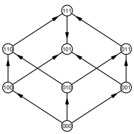
Figure 2. A fitness graph for three loci.

Results

We consider two types of fitness landscapes in our simulations: NK models and “Rough Mt. Fuji” models (e.g. Aita and Husimi,, 1996; Aita et al.,, 2000; Franke et al.,, 2011). The precise definition of both types of landscapes are found in the Appendix. Briefly, the fitnesses of genotypes in an NK landscape are determined by the fitness contribution of each locus. The fitness contribution of each locus is a stochastic function of its own state plus the state of K other loci which are fixed in advance. When K = 0, the landscape is purely multiplicative (or additive, depending on our choice of model), and (in the multiplicative case) would have no epistasis. At the other extreme, when K=N-1, the fitnesses of genotypes are mutually independent, leading to abundant epistasis.

The so called Rough Mt. Fuji models are constructed by starting with a purely additive or multiplicative model, where each allele contributes a fixed, equal amount, independent of background. The determinate fitnesses obtained this way are then perturbed by random noise. See the appendix for further details on the construction of Rough Mt. Fuji landscapes. In this study we confine ourselves to additive Rough Mt. Fuji landscapes, though we note that simulations performed with multiplicative Rough Mt. Fuji models (and which are not reported in this study) support the conclusions below. We fine tune the relative magnitudes of random noise and fixed additive contribution with a parameter, thereby allowing us to vary Rough Mt. Fuji landscapes in a manner analogous to varying NK models with the choice of K.

We will be concerned with the properties of adaptive walks in our fitness landscapes. We will assumes the asymptotic condition of Strong–Selection–Weak–Mutation (SSWM for short) (Gilliespie,, 1983, 1984; Maynard Smith,, 1970). It is assumed that the evolving population remains genetically monomorphic outside of very short time intervals, during which a new beneficial mutation sweeps to fixation. Given a genotype $g_{0}$, population genetics theory shows that if the selection coefficients of the fitter mutational neighbors $g_{1},\,g_{2},\,\ldots,\,g_{L}$ of $g_{0}$ are $s_{1},\,s_{2},\,\ldots,\,s_{L}$, respectively, then the probability of $g_{i}$ going to fixation is

$$\frac{s_{i}}{\sum_{i=1}^{n}\,s_{i}}.$$

(It should be noted that we are sweeping under the rug the fact that strictly speaking this formula is appropriate only when the magnitudes of the second or higher powers of the $s_{i}$ are negligible.) For more background about the SSWM assumption, as well as the fixation probability described, see Orr, (2002).

An adaptive walk, then, can be viewed as a stochastic path in a fitness landscape, starting at an initial genotype and ending at a genotype with locally maximal fitness. For every two steps in such a walk, three genotypes are traversed, which can be denoted, in order, $ab$, $Ab$ ,and $AB$. (Note that we are no longer assuming the minimality of $ab$ as was done in Figure 1.) These genotypes are complemented by $aB$, and the type and magnitude of epistasis for the quadruple can be determined by their fitnesses. Note that the configuration in Figure 1  D has no relevance for adaptive walks, and makes no appearance in subsequent calculations.

In Draghi and Plotkin, (2013), it was noted that the relative frequencies of sign, antagonistic, and synergistic epistasis varied along adaptive walks. Our aim is to explore this phenomenon more closely. What are the relative frequencies of sign, antagonistic, and synergistic epistasis?

In our notation, we assume that three genotypes ab, AB and AB are traversed in some adaptive walk, so that

$$w_{ab}<w_{Ab}<w_{AB},$$

and consequently $w_{aB}$ determines the type of epistasis (again, we do not assume that $w_{ab}$ is minimal). These assumptions hold for the remainder of this paper. The possibilities are that $w_{aB}$ is ranked first, second, third or fourth in terms of fitness relative to the other three genotypes. When ranked first or fourth, the quadruple has sign epistasis, and not so when ranked second or third. This fact will be used repeatedly.

We start with a preliminary observation. In the special case where fitnesses of mutational neighbors are identically and independently distributed, such as in an NK landscape with $K=N-1$, and where the genotypes are chosen randomly, the probabilities that $w_{aB}$ is ranked first, second, third or fourth are readily calculated. Indeed, the probabilities are equal, since the fitness of a paticular genotype is independent of mutational neighbors. Consequently sign epistasis occurs with frequency $0.5$.

Similarly, consider a randomly chosen quadruple but in landscapes where the fitness of mutational neighbors are correlated, as in NK landscapes with $K<N-1$. Then we expect the frequency of sign epistasis to decrease relative to the case of uncorrelated fitness. This expectation is confirmed by simulations, the results of which are found in the Appendix. The parameter ${\it slope}$ in the Rough Mt. Fuji models is positively associated with correlation between mutational neighbors. (See Appendix.) The simulation results thus confirm the expectation of lower sign epistasis in landscapes with correlated mutational neighbors.

The results of our simulations confirm Draghi and Plotkin, (2013), namely that the further one is along an adaptive walk, the larger the frequency of sign epistasis and the smaller the relative amount of antagonistic epistasis relative to synergistic epistasis. Significantly, a similar evolution of relative frequencies occurs in the Rough Mt. Fuji landscapes. It is clear that a more general explanation for this phenomenon is desirable, since Rough Mt. Fuji fitness landscapes are not defined in terms of locus–by–locus fitness contributions.

We hypothesize that the observed evolution of epistasis along adaptive walks is merely the familiar statistical phenomenon of regression to the mean. This explanation was suggested in Draghi and Plotkin, (2013) as well. However, the authors’ arguments are restricted to the details of the NK model. We offer here a simpler and more general explanation.

We begin with an intuitive explanation for the phenomenon we seek to explain. This will be followed by evidence from simulations that support our argument. We consider the type of epistasis that would be found with respect to a quadruple of genotypes $ab$, $Ab$, $aB$, and $AB$, where $ab$, $Ab$, and $AB$ form three subsequent genotypes in an adaptive walk.

Informally, the following extreme example will clarify important mechanisms. Suppose that $ab$ belongs to the highest fitness percentile among genotypes in the fitness landscape. For uncorrelated fitness, the expected frequency of sign epistasis would be at least 99 percent. Indeed, one would get $w_{aB}<w_{ab}$ in 99 percent of the cases. Similarly, for correlated fitness one would many times get $w_{aB}<w_{ab}$ as well, provided there is sufficiently much noise in the landscape. This is because a mean regression effect will tend to ”pull” $aB$ below $w_{ab}$, since $ab$ belongs to the highest fitness percentile.

After the informal example, we now go over the different possibilities for the quadruple of genotypes in some detail. We will compare low and high fitness of $ab$ with the ”null” condition where $ab$ is randomly chosen. If we impose the condition that $ab$ has lower fitness relative to the mean fitness of the landscape, then it is likely that $Ab$ and $AB$ will have lower fitness than would have been expected if $ab$ had been randomly chosen (unless the fitness landscape is uncorrelated, of course), though the likelihood of large jumps in the adaptive walk may return $AB$ to more typical fitness levels. To the extent $w_{aB}$ is determined by a stochastic component independent of $w_{ab}$, $w_{Ab}$, and $w_{AB}$, mean regression implies that it is more likely that $w_{ab}<w_{aB}$ than in the case where $ab$ is randomly chosen without condition from the fitness landscape. Note that the imposed condition of relatively low $w_{ab}$ biases the probability toward non-sign epistasis relative to the “null” condition. Furthermore, within the region of non–sign epistasis, the bias toward $w_{aB}>w_{ab}$ relative in the null situation results in a higher probability that $D=w_{AB}w_{ab}-w_{aB}w_{Ab}$ is negative, leading to a bias toward antagonistic epistasis. (One may ask about the possibility of sign epistasis where $w_{aB}>w_{AB}$. However, the fact that $w_{ab}$ is low, does not necessarily mean that $w_{AB}$ is low, as explained. In summary, we have all reasons to believe that the decrease of cases of sign epistasis where $w_{aB}<w_{ab}$ outweighs a possible increase of sign epistasis where $w_{aB}>w_{AB}$, relative the ”null” condition.)

Conversely, when an adaptive walk reaches $ab$ after a number of steps, and continues to $Ab$ followed by $AB$, it is highly likely $ab$, $Ab$, and $AB$ have high fitness relative to the mean fitness of the fitness landscape. To the extent that $w_{aB}$ is determined by a stochastic component independent of $w_{ab}$, $w_{Ab}$, and $w_{AB}$, mean regression implies that $w_{aB}<w_{ab}$ is more likely than would be the case when $ab$ is randomly chosen without condition. Furthermore, within the interval of non–sign epistasis, the quantity $D=w_{AB}w_{ab}-w_{aB}w_{Ab}$ is biased upward toward positive values, thus leading to a higher proportion of synergistic epistasis to antagonistc epistasis. We conclude that the changing balance of types of epistasis along an adaptive walk is not due to any intrinsic feature of adaptive walks per se, but rather the result of traversing from lower to higher fitnesses. Late stage adaptive walks are “walking along a ridge”, implying more sign epistasis.

In summary, the pattern of changing epistasis along an adaptive walk is driven by mean regression due to the fitnesses of $ab$, $Ab$, and $AB$ and the uncorrelated component of the fitness of $aB$.

Finally, we stress that the observed phenomenon relies on an important asymmetry between $w_{ab}$ being far below the mean, and far above the mean. Indeed, the quantity $|w_{AB}-w_{ab}|$ is expected to be relatively large for very low $w_{ab}$, and relatively small for very high $w_{ab}$. In particular, this asymmetry helps explain why one expects a prevalence of sign epistasis when $ab$ has high fitness.

Figure 3 depicts the patterns of epistasis along adaptive walks. The patterns agree well with our intuitive description. The figure concerns the NK landscape with parameters $N=15$ and $K=1$. See the Appendix for a complete description of our simulations of adaptive walks.

Figure 3. According our simulations, the patterns of epistasis change along adaptive walks as displayed. The graph depicts NK landscapes with parameters $N=15$ and $K=1$.

The case of high$w_{ab}$ is illustrated somewhat crudely in Figure 5. The blue arrows form part of an adaptive walk, and the three vertices they connect correspond to $ab$, $Ab$, and $AB$ above. If we assume that $ab$ has higher than average fitness, then when the fitness of genotype $aB$ has an uncorrelated component there is a bias toward $w_{ab}>w_{aB}$, leading to sign epistasis.

We buttressed our intuitive argument above by examining the results of simulated fitness landscapes and adaptive walks. The results of these simulations are attached as a supplement to this article. If our explanation above is correct, two results should emerge from our simulations. One, if random quadruples of genotypes as shown in Figure 1 are sampled in a stratified fashion from different fitness quartiles of the landscape, then the frequencies of sign, antagonistic, and synergistic epistasis should change their relative proportions from the lowest quartile to the highest quartile as they do along an adaptive walk. They do, as can be seen in Figure 4 and in the Appendix. (To clarify, we sampled $ab$ so that $w_{ab}$ belongs to the specified quartile. We did not impose any condition on $Ab$ and $AB$, except that $w_{ab}<w_{Ab}<w_{AB}$).

Two, if we simulate adaptive walks under the condition of equal probabilities among all mutational neighbors, the rate at which fitness increases should be slowed, and therefore the frequencies of types of epistasis should change at a slower pace than they do in a weighted probability model. They do, as can be discerned by comparing the figures with equally weighted probabilities, to the figures with probabilities weighted according to the SSWM model (see the Appendix).

Figure 4. Random quadruples were sampled in a stratified fashion, where $w_{ab}$ belongs to the specified fitness quartile. The frequencies of sign, antagonistic, and synergistic epistasis should change their relative proportions from the lowest quartile to the highest quartile as they do along an adaptive walk.

Further support for our proposed explanation was obtained by simulating 1000 $NK$ landscapes with $N=15$ and $K=10$. The result, summarized in Figure 6, confirm our assertions.

For each landscape, a genotype with relatively low fitness was chosen as the initial genotype of an adaptive walk (see Appendix for details). Figure 6 summarizes the important features of the results of the simulations. In caption A, $2.5\%-97.5\%$ percentile intervals are shown for the first($ab$), second($Ab$), and third($AB$) genotype of the adaptive walk. The fourth interval corresponds to the complementary genotype $aB$. The ranges of the intervals show a bias toward non-sign epistasis. The blue ”control” interval corresponds to randomly selected genotypes.

Conversely, in caption B, $2.5\%-97.5\%$ percentile intervals are shown for the fourth($ab$), fifth($Ab$), and sixth($AB$) genotypes visited on an adaptive walk. Again, the fourth interval corresponds to $aB$. In this case, the bias is toward high frequency of sign epistasis.

In both cases, the role of mean regression in driving the nature of epistasis along adaptive walks is apparent. s 7 and 8 represent partial views of one simulation as described above. Even here, the bias toward or away from sign epistasis depending on the stage of the adaptive walk is apparent.

We have compared equal weights, and adaptive walks under the SSWM assumption. For more background and results regarding lengths of walks, we refer to Macken and Perelson, (1989); Flyvbjerg and Lautrup, (1992) for equal weights, and Orr, (2002) for the SSWM case.

As a final remark, the study of epistasis as described was restricted to pairwise interactions. It would be interesting to extend the study to higher order interaction, and for instance to consider shapes as defined in the geometric theory of gene interactions (Beerenwinkel et al., 2007 a, ; Beerenwinkel et al., 2007 b, ).

Figure 5. Assume that the adaptive steps, colored blue, connect three genotypes with relavatively high fitness. Most connecting arrows point toward the starting point, as well as the end point of the adaptive steps. Note that due to the high fitness of the genotypes along the adaptive walk, the arrows emanating from the fourth genotype in the quadruple are more likely to point outward. The result in such a case is sign epistais.

Figure 6. 1000 adaptive walks simulated on NK landscapes with N=15 and K=10. For each walk, the starting genotype $ab$ was randomly drawn to have relatively low fitness (see Appendix for details). A. Intervals covering fitnesses between the 2.5 and the 97.5 percentiles are shown for the first (ab), second ($Ab$), and third ($AB$) genotypes in randomly generated adaptive walks, with dots indicating the medians. The genotype $aB$ is the remaining genotype in the quadruple as shown in Figure 1. The blue “Control” interval corresponds to randomly selected genotypes. The skew visible in the ab interval is due to the fact that the initial genotype of a fitness walk is drawn from a lower tail distribution. B. Intervals for the fourth, fifth, and sixth genotypes in randomly generated adaptive walks. The increased fitness of the aB genotypes in B relative to that of A is due to the fact that $K=10<14$, and thus there is some correlation between neighboring genotypes. In both diagrams, the dependency of sign epistasis on regression to the mean is apparent.

Empirical support and applications

As mentioned in the introduction, empirical data seem to support the “mean regression” hypothesis exposited herein. We add further support with the following empirical results from investigations of the TEM-family of $\beta$-lactamases (Goulart et al.,, 2013). The TEM-enzymes are associated with resistance to several $\beta$-lactame antibiotics, including penicillins. TEM beta-lactamases have been found in Escherichia coli, Klebsiella pneumoniae and other Gram-negative bacteria. TEM-1 is considered the wild-type, and approximately 200 mutant variants have been found clinically, (see e.g. the record from the Lahey Clinic http://www.lahey.org/Studies/temtable.asp).

For the 4-tuple mutant TEM-85 (L15F, R164S, E240K, T265M) the two fitness landscapes defined by Cefotaxime and Ceftazidime had mutational trajectories (i.e. adapative walks) from TEM-1 to TEM-85. For Cefotaxime there were three trajectories to TEM-85, and for Ceftazidime one trajectory. We calculated the epistasis in the last two steps, as well as in the first two steps, of the four trajectories. Fitness differences of mutational neighbors were not always statistically significant in the study, resulting in cases of “possible” sign epistasis. The results for the last two steps were two cases of sign epistasis, and two cases of possible sign epistasis. The results for the first two steps were two cases of possible sign epistasis, and two cases of no epistasis. These findings seem to support our hypothesis, though we must refrain from drawing any sweeping conclusions based on a small data set.

Generally speaking, there are two types of empirical studies of evolution, direct and indirect. A direct study is concerned with an evolving population, where mutations are observed as they occur. Examples of this are a population evolved in a laboratory or the stages of an HIV infection due to drug resistance conferring mutations. The second type of study is indirect. An investigator attempts to create a catalog of genotypes with the potential of being part of an adaptive walk. As an example, a strain of bacteria that is highly resistant to a particular antibiotic treatment may differ from the wild-type by $n$ amino acid substitutions in a relevant enzyme. The investigator in an indirect study will attempt to produce and study all $2^{n}-2$ intermediate mutational stages. It is non-trivial to relate direct and indirect studies. One wishes to infer the fitness landscape from an evolving population. Conversely, one would like to predict evolution from indirect studies. As observed in Draghi and Plotkin, (2013), epistasis may influence path choice for evolving populations, and path choice has an impact on epistasis. Consequently, it may be difficult to infer the fitness landscape from a direct study.

As for the converse, it may seem straightforward to predict evolution from a fitness landscape. However, a practical difficulty arises; namely, the information one has in an indirect study is often restricted to the fitness rankings of the genotypes, with no quantitative measurements of fitness. Consequently, one has very little knowledge of the probabilities of evolutionary trajectories, even if the fitness graph is known.

At issue here is the fact that examining epistasis in fitness graphs and evolving populations may lead to results which seem at odds. It is a priori not clear if patterns of epistasis along adaptive walks are easily predicted from fitness graphs. In addition to being used for confirming the robusticity of our results, we included the equally weighted adaptive walks (see the Appendix) to reflect the point of view of the results of an indirect study, where only the fitness rankings of the genotypes in the landscape are discovered, and thus there is no a priori knowledge of the appropriate weights to be assigned to the various paths evolution may follow.

The pattern of epistasis was broadly held across the two classes of fitness landscapes considered here, across a range of parameters for these landscapes, and across the weighted versus the unweighted versions discussed above. (The main difference we could find was pace in which proportions of epistasis changed, which is easily explained by the fact that the rate of fitness increase is slower in the equally weighted walk.) If we consider the equally weighted case as corresponding to indirect studies, and the weighted case to direct studies, then it is interesting to note while the rate of change of the proportions varies, the general pattern does not. Naturally it would be interesting to further investigate the relation between direct and indirect studies of adaptation.

Discussion

The nature of epistasis varies along an adaptive walk. This observation has been made in simulations, and has support in some empirical studies. We have argued that mean regression is a simple and general explanation for this phenomenon. We support this explanation with simulations carried out on two classes of fitness landscapes, with varying parameters. While our simulations were restricted to two classes, our argument should extend to any fitness landscape where genotypes vary to any degree independently to each other.

We considered two types of adaptives walks; those with probability weight corresponding to those used in the SSWM model, and those with equal probability weights. The similarity of the results suggests that the pattern of epistasis found along an adaptive walk is not a result of any specific property of adaptive walks generated according to the SSWM model. This result is also relevant for relating direct and indirect studies as defined above.

Further support for our assertion was obtained by sampling genotypic quadruples of mutational neighbors from simulated fitness landscapes at different fitness quartiles. The resulting pattern of increasing sign epistasis and decreasing antagonistic to synergistic ratio at higher fitnesses relative to lower fitnesses reinforces our assertion that the same phenomenon seen along adaptive walks depends on mean regression, and does not depend on any intrinsic properties of adaptive walks per se.

It should be pointed out that confidence intervals and issues with statistical power were ignored in this article. For each set of parameters, we simulated $10,\!000$ fitness landscapes with an adaptive walk. It can be seen from the figures in the Appendix that for most types of landscapes the number of adaptive walks which evolve to an $m$th genotype before hitting a local optimum decreases quite significantly with $m$ after approximately the four steps. Naturally, the low number of adaptive walks which attain higher steps may raise concerns of statistical power. Nevertheless, despite this possible shortcoming, we feel that the general pattern is clear enough.

Our main observation has important consequences for interpretations of empirical data. Consider any fitness landscape where there is a well defined wild-type, and some beneficial single mutants. For instance, the fitness landscape may be associated with antimicrobial drug resistance. Some recent papers consider prevalence of sign epistasis, and related questions for such landscapes, where the wild-type is used as a starting point (for a survey article, see Szendro et al., (e.g 2012)

Our result demonstrate that there are two factors that influence the prevalence of sign epistasis [even for a given parametric model]. The first is the degree of additivity in the landscape. The second is the fitness of the wild-type. Ideally, a study should therefore estimate wild-type fitness as well as additivity in the landscape. Roughly, one can estimate wild-type fitness from the proportion of single mutants which are more fit than the wild-type among all mutational neighbors of the wild-type (see e.g. Crona et al., (2013) for more comments).

We have argued that our main observation holds for empirical fitness landscapes. Most aspects of adaptation are sensitive for epistasis. In particular, a serious analysis of recombination, requires a fine-scaled understanding of epistasis.

Finally, our study was restricted to pairwise interactions. It would be interesting to extend the arguments given here to higher order interactions among loci.

Figure 7. A depiction of the fourth (yellow), fifth, sixth, seventh, and eighth genotype of an adaptive walk in an NK landscape, with $N=15$ and $K=10$. Only loci affected by mutation during the five adaptive steps are shown in the genotype labels, and the genotypes shown are restricted to those that differ from the initial genotype only at the five affected loci. The fitness of each genotype is also shown. The adaptive walk is colored blue, while the opposing arrows in each quadruple are colored red. Note the dominance of sign epistasis along the adaptive walk. The ridge-like quality of the adaptive walk is clear from the high proportion of “in” arrows emanating from the evolved genotypes.

Figure 8. A depiction with a description analogous to Figure 7, but in contrast, the yellow colored genotype is the initial genotype of the adaptive walk. Note the lower frequency of sign epistasis along the walk as compared to Figure 7.

Materials and Methods

Throughout this study, loci were considered to be bi–allelic, with alleles $0$ and $1$ for each locus. All of the fitness landscapes had 15 loci.

The NK model is classical. The so–called Rough Mt. Fuji model has been explored.

Some of the features of our fitness landscapes were peculiar for this study, so we will summarize briefly in this appendix how they were constructed.

For the NK fitness landscapes, the contribution of each locus is a function of the allele at the locus itself as well as the alleles at $K$ randomly chosen additional loci, or w

$$w_{j}=w_{j}(l_{j},l_{j_{1}},l_{j_{2}},\ldots,l_{j_{K}}),\quad j=1,2,\ldots,N;\quad l_{i}=0,1$$

The fitness of a particular genotype $l_{1}l_{2}\ldots l_{N}$ is then the geometric mean of the individual loci contributions:

(1) $$w(l_{1}l_{2}l_{3}\ldots l_{N})=\left(\prod_{j=1}^{N}\,w_{j}(l_{j},l_{j_{1}},l_{j_{2}},\ldots l_{j_{K}})\right)^{1/N},\quad l_{i}=0,1$$

For each of the possible values of $w_{j}$, we sampled independently from a uniform distribution over the interval $[0.05,1]$. The $0.05$ floor was used to prevent overly large fitness coefficients.

Since calculating the fitness of each genotype in an NK landscape proved computationally time–consuming, we determined the fitness quartiles theoretically as follows. Since the logarithm of the right hand side of (1) is the mean of $N$ identically distributed independent variables, by way of central limit theorem we approximated the distribution of fitnesses using a Gaussian distribution. The quartile boundaries were then determined from this approximation. Some test simulations showed this to be a reasonably accurate approximation.

To explore fully the changing nature of epistasis along an adaptive walk, for the initial genotype we sampled from genotypes with fitness below the mean minus 1.5 standard deviations according to the theoretical approximation. This corresponds (again, theoretically) to the $0.067$ quantile of the distribution.

Our Rough Mt. Fuji fitness landscapes were constructed in the spirit of their namesakes in the wider literature. At first, each genotype is assigned a deterministic fitness component given as follows:

$$\mathit{slope}\cdot\frac{\textit{\# of loci in '1' state}}{N}$$

where slope is a pre–determined fixed parameter. To each of these deterministic values a random value drawn from a uniform distribution on $[0,1]$ is added.

$$\mathit{slope}\cdot\frac{\textit{\# of loci in '1' state}}{N}+RN_{genotype}$$

Finally, we applied a linear transformation making the minimum and maximum fitnesses $0.05$ and $1$ respectively. Note that by our construction the “expected” fitness difference between the genotypes $000\ldots 0$ and $111\ldots 1$ will be $0.95\cdot{\it slope}$. The parameter slope determined the relative contributions of the deterministic component and the noise component in the landscape, with high values of slope implying a low ratio of noise component to deterministic component.

Since the computation of empirical quantiles was feasible for Rough Mt. Fuji landscapes, we used them for determining quartile boundaries and selecting initial genotypes. The latter were selected from those genotypes with fitnesses among the bottom $0.067$, as they were chosen in the $NK$ landscape case, but in this case using the empirical quantile rather than the theoretical quantile.

All simulations were coded in the programming language R.

Appendix

Table Key

In each diagram, the relative proportions are given for antagonistic, synergistic, and sign epistasis as defined in the main article. The proportions represented are among those quadruples which had epistasis. Figures 1–8 are the results of the “stratified” sampling as described in the main text. The proportions rerpresented in the “All” column are the result of 10000 simulations. Each quartile column, labeled Q1 through Q4 is the result of 2500 simulations each. In Figures 9–24, 10,000 fitness landscapes are simulated. In each, an initial genotype is selected in the manner described in the appendix. An adaptive walk is then simulated. Upon reaching the third genotype in the walk, the epistasis is calculated for that genotype and the previous two. This first calculation corresponds to Step 1 in the horizontal axis. The relative proportions of subsequent calculations of epistasis are recorded in Step 2, Step 3, etc. The meaning of the parameters used in generating the fitness landscapes is discussed in Materials and Methods.

References

- Aita and Husimi, (1996) Aita, T., Husimi, Y. (1996). Fitness spectrum among random mutants on Rough Mt. Fuji-type fitness landscape. J Theor Biol.182(4):469-85.
- Aita et al., (2000) Aita, T., Uchiyama, H., Inaoka, T., Nakajima, M., Kokubo, T. and Husimi, Y. (2000). Analysis of a local fitness landscape with a model of the rough Mt. Fuji-type landscape: application to prolyl endopeptidase and thermolysin. Biopolymers54(1): 64-79.
- (3) Beerenwinkel, N., Pachter, L. and Sturmfels, B. (2007). Epistasis and shapes of fitness landscapes. Statistica Sinica 17:1317–1342.
- (4) Beerenwinkel, N., Pachter, L., Sturmfels, B., Elena, S. F. and Lenski, R. E. (2007). Analysis of epistatic interactions and fitness landscapes using a new geometric approach. BMC Evolutionary Biology 7:60.
- Chou et al., (2011) Chou, H.H., Chiu, H.C., Delaney, N.F., Segre, D., Marx, C.J. (2011). Diminishing returns epistasis among beneficial mutations decelerates adaptation. Science 332:1190–1192.
- Crona, (2013) Crona, K. (2013) Graphs, polytopes and fitness landscapes (book Chapter), Springer, Chapter 7, 177-206. Recent Advances in the Theory and Application of Fitness Landscapes (A. Engelbrecht and H. Richter, eds.). Springer Series in Emergence, Complexity, and Computation, 2013. Springer, Chapter 7, 177-206.
- Crona et al., (2013) Crona, K., Patterson, D., Stack, K., Greene, D., Goulart, C., Mahmudi, M., Jacobs, S. D., Kallman, M. and Barlow, M. (2013) A quantification of theory-data incompatibility for fitness landscapes. arXiv:1303.3842
- Crona et al., (2013) Crona, K., Greene, D. and Barlow, M. (2013). The peaks and geometry of fitness landscapes. J. Theor. Biol. 317: 1–13.
- De Visser et al., (2009) De Visser, J. A. G. M., Park, S.C. and Krug, J.( 2009). Exploring the effect of sex on empirical fitness landscapes. The American Naturalist.
- Draghi and Plotkin, (2013) Draghi, J. A. and Plotkin, J. B. (2013). Selection biases the prevalence and type of epistasis along adaptive trajectories. Evolution doi: 10.1111/evo.12192.
- Flyvbjerg and Lautrup, (1992) Flyvbjerg, H. and Lautrup, B. (1992) Evolution in a rugged fitness landscape Physical Review A 6714-6723.
- Franke et al., (2011) Franke, J., Klözer, A., de Visser, J.A.G.M. and Krug., J. (2011). Evolutionary Accessibility of Mutational Pathways. PLoS Comput Biol 7(8): e1002134. doi:10.1371/journal.pcbi.1002134.
- Gilliespie, (1983) Gillespie, J. H. (1983). A simple stochastic gene substitution model. Theor. Pop. Biol. 23 : 202–215.
- Gilliespie, (1984) Gillespie, J. H. (1984). The molecular clock may be an episodic clock. Proc. Natl. Acad. Sci. USA 81 : 8009–8013.
- Goulart et al., (2013) Goulart, C. P., Mentar, M., Crona, K., Jacobs, S. J., Kallmann, M., Hall, B. G., Greene D., Barlow M. (2013). Designing antibiotic cycling strategies by determining and understanding local adaptive landscapes. PLoS ONE 8(2): e56040. doi:10.1371/journal.pone.0056040.
- Kauffman and Levin, (1987) Kauffman, S. A. and Levin, S. (1987). Towards a general theory of adaptive walks on rugged landscapes. J. Theor. Biol 128:11–45.
- Kauffman and Weinberger, (1989) Kauffman, S. A. and Weinberger, E.D. (1989). The NK model of rugged fitness landscape and its application to maturation of the immune response. J. Theor. Biol.;141:211–245.
- Khan et al., (2011) Khan AI, Dinh DM, Schneider D, Lenski RE, Cooper TF (2011) Negative epistasis between beneficial mutations in an evolving bacterial population. Science 332:1193–1196.
- Macken and Perelson, (1989) Macken, C. and Perelson, A. S. (1989). Protein Evolution on Rugged Landscapes. Proc Natl Acad Sci U S A. 6191-6195.
- Orr, (2002) Orr, H. A. (2001) The population genetics of adaptation: the adaptation of DNA sequences.Evolution 56:1317-1330.
- Maynard Smith, (1970) Maynard Smith, J. (1970). Natural selection and the concept of protein space. Nature 225:563–64.
- Poelwijk et al., (2007) Poelwijk, F.J., Kiviet, D. J., Weinreich, D. M. and Tans, S.J. (2007). Empirical fitness landscapes reveal accessible evolutionary paths. Nature 445:383–386.
- Poelwijk et al., (2011) Poelwijk, F. J., Sorin, T.-N., Kiviet, D. J. and Tans, S. J. (2011). Reciprocal sign epistasis is a necessary condition for multi-peaked fitness landscapes. J. Theor. Biol. Mar 7; 272(1):141–4.
- R Core Team, (2013) R Core Team (2013). R: A Language and Environment for Statistical Computing. R Foundation for Statistical Computing, Vienna, Austria. URL: http://www.R-project.org/.
- Karline Soetaert (2013) Soetart, Karline (2013). diagram: Functions for visualising simple graphs (networks), plotting flow diagrams. R package version 1.6.1. URL: http://CRAN.R-project.org/package=diagram.
- Szendro et al., (2012) Szendro, I. G., Schenk, M. F., Franke, J. Krug, J. and de Visser J. A. G. M. (2013). Quantitative analyses of empirical fitness landscapes J. Stat. Mech. P01005.
- Weinreich et al., (2005) Weinreich, D. M., Watson R. A. and Chao, L. (2005). Sign epistasis and genetic constraint on evolutionary trajectories. Evolution 59, 1165–1174.
- Wright, (1931) Wright, S. (1931). Evolution in Mendelian populations. Genetics, 16 97–159.