Covariant extrinsic gravity and the geometric origin of dark energy
Abstract
We construct the covariant or model independent induced Einstein-Yang-Mills field equations on a 4-dimensional brane embedded isometrically in an D-dimensional bulk space, assuming the matter
fields are confined to the brane. Applying this formalism to cosmology, we derive the generalized Friedmann equations. We derive the density parameter of dark
energy in terms of width of the brane, normal curvature radii and the number
of extra large dimensions. We show that dark energy could actually
be the manifestation of the local extrinsic shape of the brane. It is shown that
the predictions of this model are in good agreement with observation if we
consider an 11-dimensional bulk space.
Keywords: Extrinsic induced gravity; Extra dimensions; FLRW cosmology; Dark
energy.
PACS numbers: 04.20.-q; 04.50.-h; 95.36.+x; 98.80.-k
1 Introduction
One of the most sensational discoveries of the past decade is that the expansion of the Universe is speeding up. This observation finds support in the luminosity measurements of high redshift supernovae [1] and measurements of degree-scale anisotropies in the CMB [2]. General relativity leads to a deceleration of the expansion for the Universe if filled with cold matter or radiation. Since the expansion is speeding up, we are faced with two possibilities: The first is that 70 percent of the energy density of the Universe exists in a form with large negative pressure, called dark energy. The other possibility is that general relativity breaks down on the cosmological scales and should be modified or replaced with a more complicated theory. Various forms of modification of gravity have been proposed to explain the late time acceleration of the Universe. In an interesting development, Deffayet, Dvali and Gabadadze [3] demonstrated that the presence of the 4D Ricci scalar term in the action functional for the brane can lead to a late time acceleration [4]. The possibility that branes can naturally produce a solution to unsolved problems in gravity and cosmology, such as dark energy will generate a great boost aside from being a significant achievement in the theory and a good verification of the extra dimensions idea. With all the success that brane gravity models have achieved major weak points exist as follows;
-
•
The nature of phenomenological model building most of these theories have.
-
•
Most of the developments are specific to particular models. For example, this has given the wrong impression that the brane program is necessarily a 5D theory based on the AdS5 or Ricci flat bulk.
-
•
The geometric mechanism, like Kaluza-Klein (KK) and multidimensional gravitational models, for unification of fundamental forces, using group of isometries of non-compact bulk space is not well developed.
The general theory of relativity provides a geometric description of gravitational fields. After Einstein work, physicists have been looking for a classical unified field theory (UFT) which would describe other fundamental interactions in terms of geometric concepts of spacetime. The first attempt to set up such a UFT using the concept of adding spacelike extra dimension was that of Kaluza and Klein [5]. In KK and its multidimensional extensions the extra dimensions form a compact coset space for a given gauge group and a maximal subgroup . Consequently coordinate transformations associated with the compact manifold can be interpreted as gauge transformations.
In brane scenarios the restriction on the size of the extra dimension is weaker. Standard model and matter fields are confined to some hypersurface embedded in the bulk space. To achieve geometrical unification it is enough to consider an -dimensional brane with compact coset space embedded in -dimensional bulk space [6]. The basic difficulties of such brane models, like the original KK multidimensional theories, are the compactification of internal space, the problem of vacuum stability for the ground state, the large fermion masses which appear in nonzero modes [7] and the gauge fields appearing as the dimensional reduction are not confined to the brane and can propagate in the bulk [8]. To avoid some of the problems mentioned we need to find another geometrical origin for the gauge group of Maxwell-Yang-Mills interactions.
-
•
A simplifying assumption has been to consider the brane as highly thin. This approximation is assumed to be valid as long as the energy scales are much smaller than the energy scales related to the inverse thickness of the brane, or at distance scales much bigger than the thickness of the brane [9].
Most of the studies are restricted to thin brane models where the standard model matter fields are infinitely localized on a brane with delta-like distribution. This kind of models can, however, be only treated as an approximation since the most fundamental underlying theory (like string and quantum gravity theories) would have a minimum length scale. Also as we know, for confined standard model matter fields we have “hadron barrier” which could be encountered. Such barrier could arise because all hadrons couple via the strong interaction to low mass mesons [10]. Hence the minimum size of any physical system containing nucleons cannot be appreciably less than the range of the strong interactions [11]. The final point to note is that in thin brane approximation, in approaching the brane usually self-interactions of gravitons are divergent and consequently the justification of confined matter interactions is impossible. Consideration of a brane thickness in such models is an essential ingredient to play the role of an effective UV cut-off [12].
-
•
The main difficulty in applying a junction condition is that it is not unique. Other forms of junction conditions exist, so that different conditions may lead to different physical results [13]. Furthermore, these conditions cannot be used in the presence of more than one noncompact extra dimension.
- •
In refs. [16] and [17], the authors proposed a cosmological model for a brane embedded in a bulk space with arbitrary large extra dimensions where the matter fields are confined to the brane. As a result, an extra term in the Friedmann equation appeared that may be interpreted as the X-matter, providing a possible phenomenological explanation for the acceleration of the Universe. In this paper, we have studied the covariant (model independent) induced Einstein-Yang-Mills field equations on a 4-dimensional brane embedded isometrically in D-dimensional bulk space. The embedding is a necessity to make the Riemann curvature more consistent with the purpose of distinguishing a curved space-time from the flat space of Special Relativity. Indeed, Riemann mentions in his historical paper that his curvature cannot distinguish between a plane or a cylinder or a cone. This problem (which is in fact a topological problem in the sense of shape) was left open and a solution of it was presented by Schläfli in 1871, based on the reasoning that the local curvature cannot be an absolute concept as Riemann proposed. The curvature as a notion of shape is a relative concept, which is valid only when we have a second object to compare. Therefore, Schläfli suggested the isometric embedding of a manifold into another, so that we could always compare the curvature of that manifold with the curvature of the embedding space. The isometric condition is to guarantee that the metric of the embedded manifold is induced by the background. In our model, the extrinsic curvature plays the role of an independent field in describing dark energy. In fact, to have a common origin for the gravitational and Yang-Mills interactions we need a bulk space and consequently, the Israel junction conditions are not applicable. Also, to include the thickness of the brane we use the Nash’s theorem for perturbations of the submanifolds [18], where the extrinsic curvature and twist vector fields also play a dynamical role. Nash showed that any Riemannian geometry can be generated by a continuous sequence of infinitesimal deformations defined by the extrinsic curvature. Some popular brane-world models use M-theory motivations and use additional postulates such as a symmetry across the brane as in the Randall-Sundrum models [19]. This symmetry was not considered in this paper as essential since the symmetry breaks the regularity of the embedding, thus preventing the use of the perturbation mechanism of Nash’s theorem.
2 The geometrical aspects of model
2.1 Locally and isometrically embedding of spacetime
An effective Einstein-Hilbert action functional for the spacetime embedded in a -dimensional ambient (bulk) space may be derived from the action
| (1) |
where is the bulk space energy scale and is the Lagrangian of matter fields confined to the brane with thickness . This means that we no longer treat the confined energy-momentum tensor as a singular source, but rather as some smooth distribution along thickness of brane [20]. Variation of action (1) respect to the bulk metric with signature we obtain Einstein field equations on the bulk 111Greek indices run from 0 to 3, small case Latin indices run from 4 to and large Latin indices run from 0 to . Units so that are used throughout this work.
| (2) |
where is the bulk gravitational constant and is the confined matter energy-momentum tensor. The confinement hypothesis states that standard model matter fields are trapped to the brane with thickness . On the other hand, TeV gravitons can propagate on the bulk space freely. To construct geometrical properties of the model, we start with the local isometric embedding structure, consistent with differential structure of Einstein field equations (2).
To obtain a local and isometric embedding, consider the -dimensional Lorentzian bulk space with local coordinates , endowed with a metric . Further, consider in a submanifold with local coordinates and induced metric . We can then construct an adopted coordinate system in the bulk space which includes the local coordinates of submanifold as , where are extrinsic or extra coordinates. In such a condition the submanifold is defined by . Therefore, the isometric local embedding of a given spacetime with induced metric in an arbitrary bulk , is given by differential maps
| (3) |
Also, the vectors
| (7) |
form a basis of tangent and normal vector spaces respectively at each point of , where small Latin indices denotes extra dimensions and denotes the components of unit vector fields orthogonal to the and also normal to each other in direction of the extra coordinates . Consequently, differential map satisfies embedding equations
| (13) |
where , correspond to two possible signature of each extra dimension [25]. Note that these equations define the normal vector fields only up to . If we define the brane projections of covariant derivative of bulk space with , where is the covariant derivative compatible with , then the projected gradients of bases vectors can be decomposed with respect to the bases vectors which are the generalizations of well-known Gauss-Weingarten equations
| (17) |
where are the connection coefficients compatible with induced metric , is the extrinsic curvature (second fundamental form) of the brane
| (18) |
and is the extrinsic twist potential (third fundamental form) defined by
| (19) |
In geometric language, the presence of twist potential tilts the embedded family of submanifolds with respect to the normal vector . It is easy to show that if the bulk space has certain Killing vector fields then transform as the component of a gauge vector field under the group of isometries of the bulk [26]. Note that in our model the gauge potential can only be present if the dimension of the bulk space is equal to or greater than six , because according to (19) the twist vector fields are antisymmetric under the exchange of extra coordinate indices and .
The Lie algebra generators of are
| (20) |
and the killing vector basis of the space generated by extra dimensions are
| (21) |
A straightforward calculations show that
| (22) |
where the structure constants are
| (23) |
2.2 Geometrical structure of thick brane model
In most of brane models with single extra non compact dimension a simplifying assumption has been made to consider the brane hypersurface as extremely thin. Let us now consider a thick brane of thickness . For simplicity we will restrict ourselves to the case of constant . One way to generate such thick brane is to deform the background spacetime in such a way that it remains compatible with confinement. The embedding functions defined in (13) are differentiable and regular as required by local differentiable embedding. This follows from Nash’s embedding theorem which requires that the embedding functions of the deformed submanifold are represented by convergent positive power series [22]. According to Nash’s theorem any submanifold can be generated by a continuous sequence of small perturbations of an arbitrarily given submanifold. Although it was later generalized to pseudo Riemannian manifolds in [18]. Nash’s perturbative approach to embedding can be also described by introducing a small perturbation parameter, , along an arbitrary direction , which is parameterized by [23]. Hence, starting with the perturbation of the embedding map (1) along an arbitrary transverse direction , we obtain the coordinates of a point not necessarily on
| (31) |
where denotes the Lie derivative. The tangential projection of can always be identified with the action of brane diffeomorphism which will subsequently be ignored. Also, one can insert additional simplification by taking the norm of equal to . Hence, we can consider a general deformation along the normal vectors parameterized by extra dimensions . Consequently perturbation along orthogonal direction will be [23]
| (35) |
where denotes a small perturbation parameter. Thence the deformed embedding will be
| (39) |
where . Consequently, the set of define a Gaussian coordinate system for the bulk space in the vicinity of . The line element of bulk space in the vicinity of brane is . Now by substituting Eq. (39) in the expression for the line element, the metric of bulk space in the Gaussian coordinates will be
| (42) |
where
| (46) |
represents the metric of the brane with thickness . As one can see, equation (42) has the similar appearance to the KK metric where plays the role of the Yang-Mills potentials [24]. In fact the embedding paradigm suggests another similarity; the extrinsic shape of the brane in the neighbourhood of any of its points is determined with normal curvature [25]
| (47) |
The extreme values of normal curvature are calculated by the homogeneous equations
| (48) |
where are the curvature radii of the original brane for each principal direction and for each normal [27]. Equation (48) admits a non trivial solution for curvature directions when
| (49) |
It follows that the metric of deformed brane (46) becomes singular
at the solution of (48). Consequently according to the (42)
the metric of the bulk space also become singular at the points determined by
this solutions.
Therefore, at each point of there is a bounded coordinate
space in the normal direction generated with smallest value of the curvature radii. Hence according to the Einstein tube construction, we may associate to each point of brane a closed space generated by the normal curvature
radii.
Consequently, even though the bulk space is not compact, the local shape of the brane generates a local structure line .
Now in order to reduce the action stated in Eq. (1) in the brane, various
geometrical properties of the bulk space in the vicinity of the brane needs
to be obtained; this procedure is as follows.
Equation (39) leads to define the reference frames of the perturbed
geometry as
| (53) |
and the tangent and normal vectors to the perturbed brane respectively by
| (57) |
Hence, the embedding equations of the perturbed brane will be
| (63) |
Then the projected gradients of bases vectors can be decomposed with respect to the bases vectors which are the generalizations of Gauss-Weingarten equations for the perturbed brane
| (67) |
where are the connection coefficients compatible with induced metric , is the extrinsic curvature of the perturbed brane and . Now using the Koszul formula
| (71) |
the Gauss-Weingarten equations (67) and the fact that the commutator of two tangent vectors no longer vanishes
| (72) |
one can easily obtain the components of connection and extrinsic curvature
| (78) |
and
| (82) |
where
| (86) |
denote the total covariant (gauge covariant) derivative and horizontal lift of the base vector fields respectively. Now the geometric meaning of the second fundamental form (82) is quite clear: its symmetric part shows that the second fundamental form propagates in the bulk. The antisymmetric part is proportional to a Yang-Mills gauge field, which really can be thought of as a kind of curvature. The integrability conditions for the deformed brane are the Gauss, Codazzi and Ricci equations, respectively
| (87) |
| (88) |
| (89) |
where denotes the covariant derivative defined as
| (90) |
and is the Riemann tensor of the deformed brane
| (96) |
It is worth noticing that the Riemann tensor of the deformed brane is a reducible tensor. Again using Koszul formula we obtain
| (100) |
which helps us to obtain the remaining group of higher dimensional Riemann tensor components
| (101) |
| (102) |
| (103) |
| (104) |
| (105) |
Hence, the reduction of the Riemann tensor of the bulk space provides a generalization of the Gauss, Codazzi and Ricci equations and remaining components. Contraction of the Gauss equation (87), using equations (101) and(104) gives the Ricci scalar
| (111) |
As was mentioned earlier, the physical space on the bulk space is restricted to the Einstein tube.
3 Induced gravitational field equations on a thick brane
Now if we assume a flat bulk space with all extra dimensions being spacelike , then may be taken to be the -sphere
| (112) |
with radius . Consequently by inserting
| (113) |
and equation (111) into the action functional (2) and remembering the confinement hypothesis (matter and gauge fields are confined to the brane with thickness while gravity could propagate in the bulk space up to the curvature radii with the geometry of ) we obtain
| (119) |
where . Hence, the relation between the fundamental scale and the Planck scale will be
| (120) |
On the other hand, with an eye on the Lagrangian density of the Yang-Mills field [28]
| (121) |
the last part of (119) gives
| (122) |
where are the gauge couplings, and the index labels the simple subgroups of the gauge group. The positive constant depends on the representation symmetry group but dos not depend on the generators of Lie algebra. In adjoint representation, it can be calculated from [28]
| (123) |
Equations (23) and (123) immediately give
| (124) |
The induced gravitational “constant” is dependent on the normal curvature radii and consequently is not constant. This implies violation of the strong equivalence principle (SEP) on the brane. In scalar-tensor theories of gravity the gravitational constant having a dimension of length squared emerges through a cosmological background value of the scalar field. Also in KK and multidimensional gravitational theories with compact extra dimensions, gravitational constant is a function of the scale factor of the extra dimensions. While in our approach the extra dimensions are not compact and emerge through external shape of the brane. Equations (120) and (122) immediately give us the following fundamental relation between normal curvature radii, thickness of the brane, number of extra dimensions and Planck’s mass
| (125) |
Note that if , the above equation reduces to the equivalent relation in KK gravity [29]. To obtain the induced field equations, we only have to write the Einstein’s field equations (2) in the Gaussian frame of the bulk space. After some calculations one can obtain three sets of field equations
| (137) |
In most general cases, without assuming the existence of matter fields in the bulk space, the confinement hypothesis states that
| (143) |
The field equations (137) are equivalent to the Einstein field equations (2) representing any regular perturbation in the domain of the brane width. To establish effective induced gravitational equations for a observer living in the brane, the material (143) and geometrical quantities are defined as an average over the thickness of the brane. Hence to obtain the field equations for the covariant thick brane world model, it is sufficient to integrate field equations (137) along extra dimensions. Consequently, using (143) and (120), in the first approximation the field equations will be
| (144) |
| (145) |
| (148) |
where is the induced Einstein tensor, is the Yang-Mills energy-momentum tensor
| (149) |
and is a conserved quantity defined as
| (153) |
with direct consequence that the product of gravitational “constant” and the induced energy-momentum tensor for confined matter and Yang-Mills fields are conserved.
| (154) |
It is worth stating that the gravitational “constant” () is obtained from Eq. (120), where the curvature radius on the LHS of Eq. (120) is resulted from Eq. (49). Hence Eq. (49) plays an auxiliary role on the field equations. The extrinsic curvature can be calculated from Eqs. (145) and (153). In addition, the twist potential can be obtained from Eq. (154). Equation (148) puts a restriction on the twisting vector fields. In fact by determining the trace of Eq. (144) which gives the Ricci scalar, and plugging it in Eq (148), we have
| (155) |
Note that this is not a differential equation, but is only a restriction on the twisting vector field. This is equivalent to the equations obtained for the KK theory when the scale factor of compact space is constant, see Ref. [29]. To construct an Einstein-Yang-Mills-Scalar theory similar to the KK theory (where the LHS of equation (148) plays the role of source term) it is enough to consider a brane model with non-constant thickness. In this paper we considered a brane model for a weak field approximation with constant thickness for brane to illustrate how the extrinsic shape of brane can explain the late time acceleration of the universe.
4 The FLRW brane
4.1 Induced field equations on FLRW brane
Phenomenological fluid models of dark energy are difficult to motivate. Usually such models are unstable under perturbations, since the adiabatic speed of sound is imaginary for negative
| (156) |
Hence for constant and negative values of the model is physically not viable. In what follows we will construct a geometrical fluid with constant as a replacement of the phenomenological fluid.
First, we will analyze the influence of the extrinsic curvature terms on a FLRW Universe when all extra dimensions are spacelike. Also for simplicity, we assume that the twisting vector fields vanish. Recall that the standard FLRW line element is spatially homogeneous and isotropic which can be written as
| (157) |
where is the cosmic scale factor and is or , corresponding to the closed, open, or flat Universes. To be consistent with symmetries of the embedded FLRW Universe, the energy-momentum tensor, , must be diagonal. Hence, in the simplest realization, we have
| (163) |
where is the pressure along the extra dimensions. The general solution of equations (145) is
| (167) |
where are arbitrary functions of the cosmic time , and is the Hubbel parameter. The symmetries of spacetime encourage to assume that the functions are considered as equal; . If we set and , the components of defined in (153) will be
| (171) |
where . It can be directly verified that the conservation of is satisfied trivially without bringing up a new differential equation for obtaining . To obtain gravitational constant, it is necessary to obtain the extrinsic curvature radii of FLRW Universe from equation (49). One can easily show
| (175) |
Thence, if we assume , the normal curvature radii will be
| (176) |
Therefore according to (120) the induced gravitational “constant” is not actually a true constant and dependents on the local normal radii of the FLRW submanifold as
| (177) |
where is the present value of and
| (178) |
is the gravitational constant at the present epoch. Note that the behaviour of near a spacetime singularity depends on the topological nature of that singularity. In the point-like singularity (like FLRW case) all values of tend to zero so that also tends to zero. Therefore by inserting (171) and (177) into (144), the Friedmann equations will be
| (182) |
Also Eq. (155) gives
| (183) |
which shows that the pressure along the thickness of brane is proportional to the pressure and energy density of ordinary matter. In fact, Eq. (183) is due to the constant thickness of the brane. indicates the is an affect of constant thickness of brane. In general the RHS of this equation is proportional to the dynamics of thickness, and consequently the LHS is a source for the dynamics of the thickness. Our assumption on the constancy of thickness hence gives a simple restriction on the pressure component of the confined matter fields along the extra dimensions. Also the modified conservation of the energy-momentum tensor (154) plus equation of state for prefect fluid implies
| (184) |
where by inserting (177) on it gives
| (185) |
The Friedmann equations (182) depends on the radial bending function which remains arbitrary and dose not have a corresponding differential equation. The field equations in (145) are first order partial differential equations and do not determine uniquely the components of the extrinsic curvature. According to (18), the extrinsic curvature is dependent on the metrical structure and embedding functions . Therefore, the components of the extrinsic curvature can be calculated uniquely when the metrics of bulk and brane spaces are uniquely specified. In brane models, we have only one non-compact extra dimension, where by using the junction conditions one can obtain the components of extrinsic curvature. But here we have more than one extra dimension and consequently it is impossible to obtain the extrinsic curvature with the same methods. Hence to obtain the components of extrinsic curvature we need extra assumptions or conditions. For example if we assume that the SEP is confirmed on the brane, the gravitational constant would be really a constant and therefore the curvature radii will be fixed. This makes the bending function to be constant. Note that it has been also stated that the extrinsic curvature may satisfies the external Gupta’s equations [30] as extra condition. In Friedmann equations (182), practically we need the curvature radii not the extrinsic curvature components.
According to relation (177) the gravitational constant is a function of cosmic time and consequently the SEP is violated on the brane. The SEP comprises two assumption: that the weak equivalence principle holds, and that all local experiments (gravitational or non-gravitational) are independent of where and when in the Universe they are performed. If SEP holds on the FLRW brane, then must be constant or equivalently the brane will be umbilic. Furthermore, one experiment is not sufficient to test the SEP; at last two experiments are needed at two different times. Hence what is physically relevant is .
Using equation (177) we have
| (186) |
Several constraints on the local rate of change of using observation of lunar occultations and eclipses, gravitational lensing, evolution of the Sun, planetary and lunar radar-ranging measurements, Viking landers or data from the binary pulsar PSR 1913+16 have been obtained up to now. Among these measurements, the last one provided the most reliable upper bound [31]
| (187) |
On the other hand, the best upper bound has been obtained using helioseismological data [32]
| (188) |
At cosmological distances the best upper bound comes from the Hubble diagram of distant type Ia supernovae [33]
| (189) |
All these upper bounds are negative and shows that in the simplest model may vary as [34]
| (190) |
where is a small positive dimensionless constant. This assumption with (186) leads us to
| (191) |
Inserting (191) into (182), the Freidmann equations will be
| (195) |
4.2 The acceleration universe
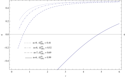
For a rough estimate consider a spatially flat brane composed of cold dark matter. In this case, the deceleration parameter reads
| (196) |
where
| (200) |
The critical case , describes a coasting cosmology instead of being supported by K-matter [35]. It is also interesting that even negative values of are allowed for dust filled Universe, since the case can be satisfied if which is in line with recent measurements using Type Ia supernovae. The deceleration parameter as a function of the redshift for some selected values of the number of the extra dimensions, , are displayed in Fig. 1. It is of some interest to determine the redshift of the deceleration-acceleration transition predicted to exist in our model. If we set (see equation (215)), the transition redshift from cosmic deceleration to acceleration for a bulk space will be which is in good agreement with the recent observations [36].
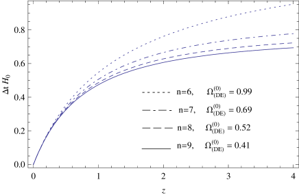
Also the lookback time, , in this model (flat case) will be
| (201) |
which shows the difference between the age of the Universe at the present epoch and when a light ray at redshift was emmited. Choosing in (201) we have the present age of the Universe. The lookback time curves as a function of the redshift for some selected values of the number of the extra dimensions, , are displayed in Fig. 2.
Note that the geometric term obtained in (171) can be rewritten as
| (202) |
One can define the corresponding perfect fluid energy-momentum tensor with geometric origin as
| (208) |
where and are the energy density and the pressure of the extrinsic dark fluid respectively, with the equation of state parameter
| (209) |
Therefore, it seems that from the point of view of a observer, the effect of the extrinsic shape of a brane looks like a perfect fluid with negative pressure.
The current value of the normal curvature radii of the FLRW Universe using (125) will be
| (210) |
which by inserting into (200) gives the current value of the density parameter of dark energy as
| (211) |
The width of the brane , can be taken as a fundamental length related to the minimum size of the confined standard model interactions, where in the present cosmological settings, should be taken as localized baryonic matter (nucleons). In the strong interactions physics, it is widely believed that coupling to the lowest mass mesons determines the localization size of hadrons to be in the manner first described by Yokawa [10]. Further evidence in support of the idea that all hadrons, e.g. nucleons, couple strongly to low mass mesons is the fact that pions are the principal secondary component in high-energy collisions [37]. Also, as we know, the strong coupling of hadrons to light mesons is a general phenomena. These considerations, together with Gell-Mann’s totalitarian principle lead Bahcall and Frantschi to the concept of “hadron barrier”: The minimum size of any system containing a nucleon cannot then be appreciably less than the range of the strong interaction of pions with nucleons i.e. [38]. Therefore, the minimum measurable length over which matter fields can be localized on the brane is of the order of their Compton wavelength of pion [39]. Also it is close to the radius of confinement, holding gluons and quarks inside hadrons [40]. Hence one may assume the width of the brane is of order of the Compton wavelength of the pion , or in a better approximation, the overlap of the quark and antiquark wave-functions in the pion, called the decay constant [41] (all hadrons have a size ). Therefore we set
| (212) |
and , the strong interaction pion-nucleon coupling “constant” [42]. Also, the best fit from the Planck temperature data with Planck lensing gives [43]. Hence the normal curvature radii at the present epoch will be
| (213) |
In 1921, Kaluza suggested to unify the gravitational and electromagnetic interaction within the framework of a five multidimensional gravity theory. The fifth coordinate was made invisible through the cylinder condition: it was assumed that in the fifth direction, the world curled up into a cylinder of very small radius (Planck’s length). In modern extension of KK ideas, the extra dimensions can be large and sometimes non-compact and the typical length of the extra dimensions will be of order [44]. For , the radius of internal space will be of order cm. This is approximately the diameter of the solar system, quite unsuitable as an internal dimension. On the other hand if , we obtain the sub-millimeter size for the internal space. According to (213), the normal radii (a reasonable distance in the bulk space for gravity) of brane in our model is of order of the Hubble distance, like Deffayet, Dvali and Gabadadze model [3]. Also the density parameter of dark energy becomes
| (214) |
Besides the BBN bound, namely
| (215) |
is also comparable with inequalities (187)-(190) help us to estimate .
The energy density of dark energy at the present epoch will be
| (217) |
Let us point out that, nearly half a century ago, an interpretation of the cosmological constant through vacuum energy density was pioneered by Zeldovich [45]. He conjectured
| (218) |
where is the cosmological constant and is close to the pion mass. Note that, the Zeldovich conjecture predicts a constant vacuum energy density, while equation (217) (which is an amendment to his conjecture) indicates a dark energy density which is not constant but changes with the expansion of the Universe.
In the following table, we find the density parameter of dark energy, age of the Universe and state parameter of dark energy for some specific number of extra dimensions.
Table (I)
| n | Age of Universe | ||
|---|---|---|---|
| 6 | 0.99 | 28.80 Gyr | -0.9989 |
| 7 | 0.69 | 13.73 Gyr | -0.9990 |
| 8 | 0.52 | 12.09 Gyr | -0.9992 |
| 9 | 0.41 | 11.35 Gyr | -0.9993 |
As one can see in table (I), the case of ( bulk space) is particularly interesting. The contribution of baryonic and cold dark matters is nothing for , . On the other hand, observations do not agree with the theoretically obtained value of the age of Universe and density parameter for . While for , not only the density fraction, age of the Universe and the equation of state parameter are in good agreement with observations and results of the Planck temperature data with Planck lensing [43], but also they have the maximum possible values. The spacial case of ambient space not only is in agreement with observations but also has deeper geometrical meaning in our model. As was mentioned in the third item of introduction, one of our goals in this paper was to find a geometrical mechanism for unification of fundamental forces, using the group of isometries of the non-compact ambient space. As shown in [46], we need at least seven non-compact extra dimensions to realize the standard Model group . The question of the true dimensionality of the world is surely one of the deepest questions that one can possibly ask in physics. Strong motivation for considering space as multidimensional comes from theories which incorporate gravity in a reliable manner; string theory and M-theory. As we know, to facilitate the construction of supersymmetry and supergravity Lagrangians, we need spacetime which is now recognized as the low energy effective description of M-theory [47]. Also to construct consistent superstring theories, the requirement is a spacetime. M-theory is an extension of superstring theory, where proponents believe that the theory unifies all five string theories. The idea is the unique supersymmetric theory in , with its low-entropy matter content and interactions fully determined, and can be obtained as the strong coupling limit of type IIA string theory because a new dimension of space emerges as the coupling constant increases [48]. As we know, the various superstring theories are related by dualities which allow the description of an object in one string model to be related to the description of a different object in another one. These dualities imply that each of string theories is a different manifestation of a single underlying M-theory. All in all, one may conclude that perhaps the real “home” of string theory is not , but possibly M-theory which could be reduced down to supergravity as well as string theory.
5 Concluding remarks
We have derived the covariant gravitational equations of a brane world model embedded isometrically in a bulk space with arbitrary number of dimensions. The extrinsic shape of the brane has a fundamental role in our approach. It makes a similarity between KK gravity and modern embedding program. Also the induced gravitational constant depends on the extrinsic shape of our Universe. The gravitational model thus obtained was then applied to cosmology. Assuming the FLRW spacetime embedded isometrically in a bulk space with arbitrary spacelike extra dimensions, we have re-derived the generalized Friedmann equations. The obtained field equations contain the geometric fluid with its properties related to the extrinsic shape of the brane via the gravitational “constant”. Hence, from point of view of a confined observer, (which does not have access to the extra dimensions), the late time acceleration of the Universe looks like as the effect of some phenomenological dark fluid.
6 Acknowledgements
We thank H. R. Sepangi and M. D. Maia for comments and suggestions.
References
- [1] S. Perlmutter, G. Aldering, G. Goldhaber, et al. Astrophys. J. 517 (1999) 565; A.G. Riess, A.V. Filippenko, et al. Astron. J. 116 (1998) 1009.
- [2] D.N. Spergel, et al. (WMAP), Astrophys. J. Suppl. 148 (2003) 175.
- [3] C. Deffayet, G. Dvali and G. Gabadadze, Phys. Rev. D 65 (2002) 044023; C. Deffayet, S.J. Landau, J. Raux, M. Zaldarriaga and P. Astier, Phys. Rev. D 66 (2002) 024019.
- [4] G. Dvali and G. Gabadadze, Phys. Rev. D 63 (2001) 065007; C. Deffayet, Phys. Lett. B 502 (2001) 199.
- [5] T. Kaluza, Sitzungber, Preass Akad. Wiss. Berlin Math. Phys. K1 (1921) 966; O. Klein, Z. Phys. 37 (1926) 895.
- [6] T. Han, J. D. Lykken and R. Zhang, Phys. Rev. D 59 (1999) 105006; G. Papadopoulos and P. K. Townsend, Phys. Lett. B 393 (1997) 59; M. Cvetic, H. Lu and C. N. Pope, J. Math. Phys. 42 (2001) 3048.
- [7] N. Arkani-Hamed and M. Schmaltz, Phys. Rev. D 61 (2000) 033005.
- [8] A. Neronov, Phys. Rev. D 64 (2001) 044018.
- [9] P. Mounaix and D. Langlois, Phys. Rev. D 65 (2002) 103523; S. Khakshournia, Gen. Relativ. Gravit. 40 (2008) 1791; V. Dzhunushaliev, V. Folomeev, K. Myrzakulov and R. Myrzakulov, Gen. Relativ. Gravit. 41 (2009) 131; R. Casadio, B. Harms and O. Micu, Phys. Rev. D 82 (2010) 044026.
- [10] H. Yokawa, Proc. Phys. Math. Soc. Jpn. 17 (1935) 48.
- [11] D.F. Falla and P.T. Landsberg, Nuovo Cimento B 106 (1991) 669.
- [12] V. Dzhunushaliev, V. Folomeev and M. Minamitsuji, Rept. Prog. Phys. 73 (2010) 066901 [arXiv:0904.1775 [gr-qc]].
- [13] R. A. Battye and B. Carter, Phys. Lett. B 509 (2001) 331.
- [14] M. Fairbairn and A. Goobar, Phys. Lett. B 642 (2006) 432; R. Maartens and E. Majerotto, Phys. Rev. D 74 (2006) 023004; U. Alam and V. Sahni, Phys. Rev. D 73 (2006) 084024; Y.S. Song and I. Sawicki and W. Hu, Phys. Rev. D 75 (2007) 064003.
- [15] A. Nicolis and R. Rattazzi, J. High Energy Phys. 0406 (2004) 059; M.A. Luty, M. Porrati and R. Rattazzi, J. High Energy Phys. 0309 (2003) 029.
- [16] M.D. Maia, E.M. Monte, J.M.F. Maia and J.S. Alcaniz, Class. Quantum Grav. 22 (2005) 1623.
- [17] M. Heydari-Fard, M. Shirazi, S. Jalalzadeh and H.R. Sepangi, Phys. Lett. B 640 (2006) 1.
- [18] J. Nash, Ann. Maths., 63 (1956) 20; R. Greene, Memoirs Amer. Math. Soc. 97, (1970).
- [19] L. Randall and R. Sundrum, Phys. Rev. Lett. 83 (19946909) .
- [20] B. Carter, R.A. Battye and J.P. Uzan, Comm. Matt. Phys., 235 (2003) 289.
- [21] E.M. Monte and M.D. Maia, J. Math. Phys. 37 (1996) 1972.
- [22] M.D. Maia, Int. J. Mod. Phys. A, 26 (2011) 3813.
- [23] M.D. Maia and W. Mecklenburg, J. math. Phys. 25 (1984) 3047; M.D. Maia, A.J.S. Capistrano, and D. Muller, Int. J. Mod. Phys. D 18 (2009) 1273; M.D. Maia, arXiv:0811.3835v1; A.J.S. Capistrano, and P.I. Odon, Cen. Eur. J. Phys 9 (2010) 189.
- [24] M.D. Maia, Class. Quant. Grav. 6 (1989) 173; K. Akama and T. Hattori, Mod. Phys. Lett. A 15 (2000) 2017.
- [25] L.P. Eisenhart, Riemannian Geometry Princeton U. P. Princeton, N. J. (1966).
- [26] S. Jalalzadeh, B. Vakili and H.R. Sepangi, Phys. Scr. 76 (2007) 122.
- [27] E. Kreyszig, Differential Geometry, Dover Publications, Inc., New York (1991).
- [28] F. Scheck, Classical Field Theory, Graduate Texts in Physics, Springer-Verlag Berlin Heidelberg (2012).
- [29] J.M. Overduin and P.S. Wesson, Phys. Rept. 283 (1997) 303.
- [30] M. D. Maia, A. J. S. Capistrano, J. S. Alcaniz, E. M. Monte, Gen. Rel. Grav. 43 (2011) 2685.
- [31] T. Damour, G.W. Gibbons and J.H. Taylor, Phys. Rev. Lett., 61 (1988) 1151.
- [32] D.B. Guenther, L.M. Krauss and P. Demarque, ApJ, 498 (1998) 871.
- [33] E. Gaztañaga, E. García-Berro, J. Isern, E. Bravo and I. Domínguez, Phys. Rev. D 65 (2001) 023506.
- [34] R.W. Hellings, et al., Phys. Rev. Lett. 51 (1983) 1609.
- [35] E.W. Kolb, ApJ, 344 (1989) 543.
- [36] R. Giostri, M. Vargas dos Santos, I. Waga, R. R.R. Reis, M.O. Calvão, B.L. Lago, JCAP 03 (2012) 027.
- [37] B. Yu. Bushnin, et al. Phys. Lett. B 29 (1969) 48.
- [38] J.N. Bahcall and S. Frautschi, Astrophys. J. 170 (1971) L81.
- [39] K. Nakamura, et al. (Particle Data Group), J. Phys. G, 37 (2010) 075021.
- [40] L.B. Okun, Elementary Particle Physics, Nauka, Moscow (1986).
- [41] J.L. Rosner and S. Stone, arXiv:1201.2401.
- [42] B.L. Ioffe and A.G. Oganesian, Phys. Rev. D 57, (1998) R6590; S.L. Zhu, W.Y.P. Hwang and Y.B.P. Dai, Phys. Rev. C 59 (1999) 442.
- [43] P. Ade, et al. (Planck Collaboration) (2013), arXiv:1303.5076.
- [44] N. Arkani-Hamed, et al, Phys. Lett. B 429 (1998) 263; Phys. Rev. Lett 84 (2000) 586.
- [45] Y.B. Zeldovich, Sov. Phys. Usp. 11 (1968) 381; Y. B. Zeldovich, Sov. Phys. Usp. 24 (1981) 216.
- [46] P. Maraner and J.K. Pachos, Annals Phys. 323 (2008) 2044.
- [47] E. Witten, Nucl. Phys. B 443 (1995) 85; P. Horava and E. Witten, Nucl. Phys. B460 (1996) 506; Nucl. Phys. B 475 (1996) 94.
- [48] J.H. Schwarz, Phys. Lett. B 367 (1996) 97.