CollegeOrDept University PhilosophiæDoctor (PhD) Madrid Junio de 2013

Dynamical Yukawa Couplings

Glossary
CKM - Cabibbo-Kobayashi-Maskawa [quark mixing matrix]
CP - Parity and Charge conjugation
EFT - Effective Field Theory
EWSB - Electroweak Symmetry Breaking
FCNC - Flavour Changing Neutral Current
FSB - Flavour Symmetry Breaking
$\mathcal{G}$ - Gauge Group of the Standard Model: $SU(3)_{c}\times SU(2)_{L}\times U(1)_{Y}$
$\mathcal{G}_{\mathcal{F}}$ - Flavour Group: $U(n_{g})^{5}\times O(n_{g})$
$\mathcal{G}_{\mathcal{F}}^{\not{A}}$ - Explicitly Axial Symmetry Breaking case Flavour Group: $SU(n_{g})^{5}\times SO(n_{g})$
GIM - Glashow-Iliopoulos-Maiani [mechanism]
HP - Hierarchy Problem
IH - Inverted Hierarchy
$J$ - Jacobian of the change of coordinates from the physical parameters to the invariants
LHC - Large Hadron Collider
ME - Modelo Estándar
$n_{g}$ - Number of fermion generations
NH - Normal Hierarchy
PJ - Problema de la Jerarquía
PMNS - Pontecorvo-Maki-Nakagawa-Sakata [lepton mixing matrix]
QFT - Quantum Field Theory
QCD - Quantum Chromodynamics
RESE - Rotura Espontánea de Simetría Electrodébil
SM - Standard Model
$\mathcal{Y}$ - Flavour scalar fields in the bi-fundamental representation
$\chi$ - Flavour scalar fields in the fundamental representation

1 Objetivo y motivación

El campo de física de partículas se encuentra actualmente en un punto crucial. La exploración del mecanismo de rotura espontánea de simetría electrodébil (RESE) en el gran colisionador de hadrones (LHC) ha desvelado la presencia de un bosón que se asemeja al escalar de Higgs (1, 2) dada la precisión de los datos experimentales disponibles (3, 4). La descripción del Modelo Estándar (ME) de la generación de masas (5, 6, 7) ha demostrado ser acertada y la auto-interacción del bosón de Higgs que desencadena la RESE es ahora la quinta fuerza de la naturaleza, junto con la gravedad, el eletromagnetismo la interacción débil y la fuerte.

Esta nueva fuerza, como el resto de las fuerzas cuantizadas, varía en intensidad dependiendo de la escala a la que se la examine, pero al contrario que la fuerza débil o fuerte, esto plantea un problema (8) ya que a una escala de alta energía o corta distancia del orden de $10^{-12}fm$ el mecanismo de RESE se desestabilizaría, pues el acoplo cuártico se cancelaría (9, 10). Dicho problema podría ser resuelto por la introducción de nueva física, lo cual conduce a otra cuestión teórica, el Problema de la Jerarquía (PJ). Cualquier tipo de nueva física que se acople a la partícula de Higgs produce genéricamente una contribución radiativa al término de masa de dicho bosón del orden de la nueva escala, lo que significaría que la escala electrodébil es naturalmente cercana a la escala de física más alta que interacciona con los campos del ME. Las propuestas para solucionar este problema pueden ser clasificadas en soluciones de física perturbativa, siendo el paradigma la supersimetría, y ansazts de dinámica fuerte. Supersimetría es una elegante simetría entre bosones y fermiones que implica cancelaciones sistemáticas entre las contribuciones radiativas bosónicas y fermiónicas al término de masa del Higgs. Por otro lado la hipótesis de que el bosón de Higgs sea un estado ligado producido por nueva dinámica fuerte implica que el mecanismo de RESE del ME es simplemente una descripción efectiva que debe ser completada por una teoría más fundamental. Todas estas hipótesis suponen naturalmente nueva física a la escala del TeV y están siendo testeadas de manera decisiva en el LHC.

En el frente cosmológico la interacción gravitatoria ha sido la fuente de nuevos desafíos en física de partículas. El universo está expandiéndose aceleradamente, algo que en cosmología estándar requiere la presencia de “energía oscura”, una energía de vacío cuya presión negativa provoca que el universo se ensanche con velocidad creciente. Estimaciones naif en la teoría estándar de la contribución a este tipo de energía difieren del valor observado 120 órdenes de magnitud, un hecho que muestra enfáticamente nuestra ignorancia sobre la naturaleza de la energía oscura. Cosmología y astrofísica proporcionaron la sólida evidencia de materia extra no bariónica en el universo, llamada ‘materia oscura”, como otra muestra experimental no explicable en el ME. Hay un activo programa experimental para la búsqueda de materia oscura en este dinámico sector de física de partículas. La tercera evidencia de nueva física en cosmología proviene de un hecho muy familar del mundo visible: está constituido de mucha mas materia que antimateria, y aunque el ME proporciona una fuente de exceso de partículas sobre antipartículas el resultado no es suficiente para explicar la proporción observada.

La parte de nueva física que concierne más de cerca al ME es el hecho de que los neutrinos han demostrado ser masivos. La evidencia de masa de neutrinos proveniente de los datos de oscilación es una de las selectas evidencias de nueva física mas allá del ME. En este sector la búsqueda de violación leptónica de conjugación de carga y paridad (CP), transiciones de sabor de leptones cargados y la relación fundamental entre neutrinos y antineutrinos; su carácter Majorana o Dirac, tienen ambiciosos programas experimentales que producirán resultados en los próximos años.

Para completar la lista de desafíos en física de partículas, deben ser mencionados la tarea pendiente de la cuantización de gravedad y el presente pobre entendimiento del vacío de QCD representado en el problema-$\theta$.

El tema de esta tesis es un problema horizontal: el puzle de sabor. La estructura de sabor del espectro de partículas está conectada en la teoría estándar a la RESE, y las masas de los neutrinos son parte esencial de este puzle. Éstos son temas que han sido tratados en el trabajo del estudiante de doctorado en otro contexto: la fenomenología de sabor en el caso de dinámica fuerte de RESE (11, 12), la determinación del Lagrangiano bosónico general en el mismo contexto (13) y la fenomenología de sabor de un modelo para masas de neutrinos (14) han formado parte del programa de doctorado del candidato. El tema central de esta tesis es sin embargo la exploración de una posible explicación a la estructura de sabor (15, 16, 17, 18).

El principio gauge puede ser señalado como la fuente creadora de progreso en física de partículas, bien entendido y elegantemente implementado en el ME. Por el contrario el sector de sabor permanece durante décadas como una de las partes peor entendidas del ME. El ME muestra la estructura de sabor de una manera paramétrica, dejando sin respuesta preguntas como el origen de la fuerte jerarquía en masas de fermiones o la presencia de grandes angulos de mezcla de sabor para leptones en constraste con la pequeña mezcla del sector de quarks; éstas preguntas conforman el conocido como puzle de sabor. Dicho puzle permanece por lo tanto como una cuestión fundamental sin respuesta en física de partículas.

La principal guía en este trabajo es el uso de simetría para explicar el puzle de sabor. La simetría, que juega un papel central en nuestro entendimiento en física de partículas, es empleada en esta tesis para entender la estructura de sabor. Un número variado de simetrías han sido postuladas con respecto a este problema (19, 20, 21, 22, 23, 24, 25, 26, 27, 28, 29, 30). En este estudio la simetría será seleccionada como la mayor simetría continua global posible en la teoría libre . La elección está motivada por las exitosas consequencias fenomenológicas de selectionar la susodicha simetría en el caso de la hipótesis de Violación Mínima de Sabor (23, 26, 27, 28, 29), un campo en el que el autor también a trabajado (29). Debe ser destacado que los diferentes orígenes posibles para la masa de los neutrinos resultan en distintas simetrías de sabor en el sector leptónico; de especial relevancia es la elección del carácter Dirac o Majorana. En cualquiera de los casos la simetría de sabor no es evidente en el espectro, luego debe estar escondida. En este trabajo el estudio de rotura espontánea de la simetría de sabor para leptones y quarks será desarrollado con énfasis en el resultado natural contrastado con la estructura observada en la naturaleza. Se mostrará como la diferencia entre quarks y leptones en la estructura de sabor resultante, en particular los ángulos de mezcla, se origina en la naturaleza Majorana o Dirac de los fermiones.

En el presente análisis, el criterio de naturalidad será la regla para decidir si la solución propuesta es aceptable o introduce puzles mas complicados que los que resuelve. Es relevante por lo tanto la acepción de naturalidad, siguiendo el criterio de t’Hooft, todos los parámetros adimensionales no restringidos por una simetría deben ser de orden uno, mientras que todos los parámetros con dimesiones deben ser del orden de la escala de la teoría. Exploraremos por lo tanto en qué casos este criterio permite la explicación de la estructura de masas y angulos de mezcla.

Respecto a las diferentes partes de nueva física involucradas conviene distinguir tres escalas distintas i) la escala de RESE establecida por la masa del bosón W, ii) un escala posiblemente distinta de sabor, denotada $\Lambda_{f}$ y característica de la nueva física responsable de la estructura de sabor, iii) la escala efectiva de violación de numero leptónico $M$ responsable de las masas de los neutrinos, en el caso de que éstas sean de Majorana.

2 Aim and Motivation

The field of particle physics is presently at a turning point. The exploration of the mechanism of electroweak symmetry breaking (EWSB) at the LHC has unveiled the presence of a boson with the characteristics of the Higgs scalar (1, 2) given the precision of presently available data (3, 4). The Standard Model (SM) description of mass generation (5, 6, 7) has proven successful, and the Higgs self-interaction that triggers EWSB stands now as the fifth force in nature, after gravity, electromagnetism, weak and strong interactions.

This new force, as every other quantized force in nature, varies in strength depending on the scale at which it is probed but, unlike for strong or weak forces, this poses a problem (8) as at a high energy or short distance scale of order $10^{-12}fm$ the mechanism of electroweak symmetry breaking would be destabilized since the coupling of this force vanishes (9, 10). This problem could be solved by the introduction of new physics which brings the discussion to another theoretical issue, the Hierarchy Problem. The point is that any new physics that couples to the Higgs particle produces generically a radiative contribution to the Higgs mass term of order of the new mass scale, which would mean that the electroweak scale is naturally close to the highest new physics scale that couples to the SM fields. Proposals to address this problem can be classified in perturbative physics solutions, the paradigm being supersymmetry, and strong dynamics ansatzs. Supersymmetry is an elegant symmetry between bosons and fermions that implies systematic cancellations among the contributions to the Higgs mass term of these two types of particles. On the other hand the hypothesis of the Higgs boson being a bounded state produced by new strong dynamics implies that the mechanism of electroweak symmetry breaking of the SM is just an effective description to be completed by a more fundamental theory. All these hypothesis involve new physics at the TeV scale and are being crucially tested at the LHC.

In the cosmology front, the gravitational interaction has been the source of new challenges in particle physics. The universe is accelerating, something that in standard cosmology requires the presence of “Dark Energy”: a vacuum energy whose negative pressure makes the universe expand with increasing rate. Naive estimates of the contribution to this type of energy from the standard theory are as far off from the observed value as $120$ orders of magnitude, a fact that emphatically reflects our ignorance of the nature of Dark Energy. Furthermore cosmology together with astrophysics brought the solid piece of evidence of extra matter in the universe which is not baryonic, the so called “Dark Matter” as another experimental evidence not explainable within the Standard Model. There is an active experimental program for the search of Dark Matter in this lively sector of particle physics. The third piece of evidence of new physics in cosmology stems from one very familiar fact of the visible universe: it is made out of much more matter than antimatter, and even if the SM provides a source for particle over antiparticle abundance in cosmology, this is not enough to explain the ratio observed today.

The evidence of new physics that concerns more closely the Standard Model is the fact that neutrinos have shown to be massive. The data from oscillation experiments revealed that neutrinos have mass, a discovery that stands as one of the selected few sound pieces of evidence of physics beyond the SM. In this sector the search for leptonic CP violation, charged lepton generation transitions and most of all the fundamental relation among neutrino particles and antiparticles; their Majorana or Dirac nature, are exciting and fundamental quests pursued by ambitious experimental programs.

To complete the list of challenges in particle physics, it shall be mentioned that there is the pending task of the quantization of gravity and the present poor understanding of the vacuum of QCD embodied in the $\theta$ problem.

The focus of this project is a somehow horizontal problem: the flavour puzzle, which is constituted by the mass and mixing pattern of the known elementary fermions. The flavour structure of the particle spectrum is connected in the standard theory to EWSB, and the masses of neutrinos are an essential part of the flavour puzzle. EWSB and neutrino masses have been subject of study in a different context for the PhD candidate: the flavour phenomenology in a strong EWSB realization (11, 12), the determination of the general bosonic Lagrangian in the same scheme (13) and the flavour phenomenology of a neutrino mass model (14) are part of the author’s work. The focus of this write-up is nonetheless on the exploration of a possible explanation of the flavour pattern developed in Refs. (15, 16, 17, 18).

The gauge principle can be singled out as the driving engine of progress in particle physics, well understood and elegantly realized in the SM. In contrast the flavour sector stands since decades as the less understood part of the SM. The SM displays the flavour pattern merely parametrically, leaving unanswered questions like the origin of the strong hierarchy in fermion masses or the presence of large flavour mixing in the lepton sector versus the little overlap in the quark sector. The flavour puzzle stays therefore a fundamental open question in particle physics.

The main guideline behind this work is the use of symmetry to address the flavour puzzle. Symmetry, that plays a central role in our understanding of particle physics, is called here to explain the structure of the flavour sector. A number of different symmetries have been postulated with respect to this problem (19, 20, 21, 22, 23, 24, 25, 26, 27, 28, 31, 29, 30). Here the symmetry will be selected as the largest possible continuous global symmetry arising in the free theory . This choice is motivated by the successful phenomenological consequences of selecting this symmetry, as in the case of the Minimal Flavour Violation (MFV) ansatz (23, 26, 27, 28, 31, 29), a field to which the author has also contributed (29). It must be underlined that the different possible origins of neutrino masses result in different flavour symmetries in the lepton sector; of special relevance is the choice of Majorana or Dirac nature. The flavour symmetry in any case is not evident in the spectrum, ergo it must be somehow hidden.

In this dissertation the study of the mechanism of flavour symmetry breaking for both quark and leptons will be carried out with emphasis on its natural outcome in comparison with the observed flavour pattern. It will be shown how the difference between quark and leptons in the resulting flavour structure, in particular mixing, stems from the Majorana or Dirac nature of fermions.

In the analysis presented here, naturalness criteria shall be the guide to tell whether the implementation is acceptable or introduces worse puzzles than those it solves. A relevant issue is what will be meant by natural; following ’t Hooft’s naturalness criteria, all dimensionless free parameters not constrained by a symmetry should be of order one, and all dimensionful ones should be of the order of the scale of the theory. We will thus explore in which cases those criteria allow for an explanation of the pattern of mixings and mass hierarchies.

As for the different physics involved in this dissertation, there will be three relevant scales; i) the EWSB scale set by the $W$ mass and which in the SM corresponds to the vacuum expectation value (vev) $v$ of the Higgs field; ii) a possible distinct flavour scale $\Lambda_{f}$ characteristic of the new physics underlying the flavour puzzle; iii) the effective lepton number violation scale $M$ responsible for light neutrinos masses, if neutrinos happen to be Majorana particles.

3 Introduction

As all pieces of the Standard Model fall into place when confronted with experiment, the last one being the discovery of a Higgs-like boson at the LHC (1, 2), one cannot help but stop and wonder at the theory that the scientific community has carved to describe the majority of phenomena we have tested in the laboratory. This theory comprises both the forces we have been able to understand at the quantum level and the matter sector. The former shall be briefly reviewed first.

3.1 Forces of the Standard Model

Symmetries have shed light in numerous occasions in particle physics, in particular the understanding of local space-time or gauge symmetries stands as the deepest insight in particle physics. The gauge principle, at the heart of the SM, is as beautifully formulated as powerful and predictive for describing how particles interact through forces. The SM gauge group,

$$\mathcal{G}=SU(3)_{c}\times SU(2)_{L}\times U(1)_{Y}\,,$$ (3.1)

encodes the strong, weak and electromagnetic interactions and describes the spin 1 (referred to as vector-boson) elementary particle content that mediate these forces. The strong interactions concern those particles that transform under $SU(3)_{c}$ with $c$ standing for color, and are the subject of study of quantum chromodynamics (QCD). The electroweak sector $SU(2)_{L}\times U(1)_{Y}$ comprises the weak isospin group $SU(2)_{L}$ and the abelian hypercharge group $U(1)_{Y}$ which reduce to the familiar electromagnetic gauge group and Fermi interaction below the symmetry breaking scale. This part of the theory is specified, in the unbroken phase, given the group and the coupling constants of each subgroup, here $g_{s}$ for $SU(3)_{c}$, $g$ for $SU(2)_{L}$ and $g^{\prime}$ for $U(1)_{Y}$ at an energy scale $\mu$. This information is enough to know that 8 vector-boson mediate the strong interaction, the so-called gluons, and that 4 vector bosons enter the electroweak sector: the $Z,W^{\pm}$ and the photon.

The implementation of the gauge principle in a theory that allows the prediction of observable magnitudes as cross sections, decay rates etc. makes use of Quantum Field Theory (QFT). In the canonical fashion we write down the Lagrangian density denoted $\mathscr{L}$, that for the pure gauge sector of the Standard Model reads:

$$\mathscr{L}_{gauge}=-\frac{1}{2}\mbox{Tr}\left\{G^{\mu\nu}G_{\mu\nu}\right\}-\frac{1}{2}\mbox{Tr}\left\{W^{\mu\nu}W_{\mu\nu}\right\}\,-\frac{1}{4}B^{\mu\nu}B_{\mu\nu},$$ (3.2)

where and $\mu$ and $\nu$ are Lorentz indexes and $G_{\mu\nu},W_{\mu\nu}$ and $B_{\mu\nu}$ stand for the field strengths of $SU(3)_{c}\,,\,SU(2)_{L}$ and $U(1)_{Y}$ respectively. This part of the Lagrangian describes forces mediators and these mediators self-interaction. The field strengths are defined through the covariant derivatives:

$$D_{\mu}=\partial_{\mu}+ig_{s}\frac{\lambda_{i}}{2}G_{\mu}^{i}+ig\frac{\sigma_{i}}{2}W^{i}_{\mu}+ig^{\prime}Q_{Y}B_{\mu}\,,$$ (3.3)

with Gell-Mann matrices $\lambda_{i}$ as generators of color transformations, Pauli matrices $\sigma_{i}$ as weak isospin generators, and $Q_{Y}$ is the hypercharge of the field that the covariant derivative acts on. $G_{\mu}^{i}$ denote the 8 gluons, $W^{i}_{\mu}$ the three weak isospin bosons and $B_{\mu}$ the hypercharge mediator. The photon ($A_{\mu}$) and $Z$ are the usual combination of neutral electroweak bosons: $Z_{\mu}=\cos\theta_{W}W_{\mu}^{3}-\sin\theta_{W}B_{\mu}$, $A_{\mu}=\sin\theta_{W}W_{\mu}^{3}+\cos\theta_{W}B_{\mu}$ and the weak angle, $\tan\theta_{W}=g^{\prime}/g$. In terms of the covariant derivatives the field strengths are defined as:

$$G_{\mu\nu}=-\frac{i}{g_{s}}\,\left[D_{\mu},D_{\nu}\right]\,,\quad W_{\mu\nu}=-\frac{i}{g}\,\left[D_{\mu},D_{\nu}\right]\,,\quad B_{\mu\nu}=-\frac{i}{g^{\prime}}\,\left[D_{\mu},D_{\nu}\right]\,,$$ (3.4)

where the covariant derivative acts on a fundamental or unit-charge implicit object of the corresponding gauge subgroup. However the fact that the $W$ and $Z$ spin-1 bosons are massive requires of the introduction of further bosonic fields in the theory. This brings the discussion to the electroweak breaking sector. Masses are not directly implementable in the theory as bare or “hard” mass terms are not allowed by the gauge symmetry. The way the SM describes acquisition of masses is the celebrated Brout-Englert-Higgs mechanism (5, 6, 7), a particularly economic description requiring the addition of a $SU(2)_{L}$ doublet spin-0 boson (scalar), denoted $H$. This bosonic field takes a vev and its interactions with the rest of fields when expanding around the true vacuum produce mass terms for the gauge bosons. The interaction of this field with the gauge fields is given by its transformation properties or charges, reported in table 3.1, the masses produced for the $W$ and $Z$ boson being in turn specified by the vev of the field $\left\langle H\right\rangle\equiv(0,v/\sqrt{2})^{T}$ together with the coupling constants $g$ and $g^{\prime}$.

	$SU(3)_{c}$	$SU(2)_{L}$	$U(1)_{Y}$
$H$	1	2	1/2

Table 3.1: The Higgs field charges under $\mathcal{G}$

This vev is acquired via the presence of the quartic coupling of the Higgs, the fifth force, and the negative mass term. These two pieces conform the potential that triggers EWSB and imply the addition of two new parameters to the theory, explicitly:

$$\mathscr{L}_{H}=\left(D_{\mu}H\right)^{\dagger}D^{\mu}H-\lambda\left(H^{\dagger}H-\frac{v^{2}}{2}\right)^{2}\,.$$ (3.5)

where the $v$ is the electroweak scale $v\simeq 246$GeV and $\lambda$ the quartic coupling of the Higgs, which can be extracted from the measured Higgs mass $\lambda=m_{h}^{2}/(2v^{2})\simeq 0.13$. Note that the potential, the second term above, has the minimum at $\left\langle H^{\dagger}H\right\rangle=v^{2}/2$.

As outlined in the previous section, the Higgs could be elementary or composite; the paradigm of composite bosons are pions, understood through the Goldstone theorem. In the pions chiral Lagrangian the relevant scale is the pion decay constant $f_{\pi}$ associated to the strong dynamics, in the analogy with a composite Higgs the scale is denoted $f$ which, unlike in technicolor (32, 33, 34), in Composite Higgs Models (35, 36, 37, 38, 39) is taken different from the electroweak vev $v$. In the limit in which these two scales are close, a more suitable parametrization of the Higgs is, alike to the exponential parametrization of the $\sigma$-model,

$$\left(\tilde{H}\,,\,H\right)=U\,\frac{\left\langle h\right\rangle+h}{\sqrt{2}}\,,\qquad\qquad U^{\dagger}U=UU^{\dagger}=1\,,$$ (3.6)

where $\tilde{H}=i\sigma_{2}H^{*}$ with $\sigma_{2}$ the second Pauli matrix in weak isospin space. $U$ is a $2\times 2$ unitary matrix which can be thought of as a space-time dependent element of the electroweak group and consequently absorbable in a gauge transformation while $\left\langle h\right\rangle+h$ is the constant “radial” component plus the physical bosonic degree of freedom, both invariant under a gauge transformation. The value of $\left\langle h\right\rangle$ is fixed by $v$ and $f$.

In this way gauge invariance of the corrections to Eq. 3.5 concerns the dimensionless $U$ matrix and its covariant derivatives whereas the series in $H/f$ can be encapsulated in general dimensionless functions $\mathcal{F}[(\left\langle h\right\rangle+h)/f]$ different for each particular model.

Since both $U$ and $\mathcal{F}$ are dimensionless, the expansion is in powers of momentum (derivatives) over the analogous of the chiral symmetry breaking scale (40, 41). The Lagrangian up to chiral dimension 4 in this scheme for the bosonic sector was given in (13) and the flavour phenomenology in this scenario was studied in (11, 12) as part of the authors work that however does not concern the discussion that follows.

3.2 Matter Content

The course of the discussion leads now to the matter content of the Standard Model. Completing the sequence of intrinsic angular momentum, between the spin 1 vector bosons and the spin 0 scalars, the spin $1/2$ ultimate constituents of matter, the elementary fermions, are placed. These fermions constitute what we are made of and surrounded by. Their interactions follow from their transformation properties under the gauge group. Quarks are those fermions that sense the strong interactions and are classified in three types according of their electroweak interactions; a weak-isospin doublet $Q_{L}$ and two singlets $U_{R},D_{R}$ . Leptons do not feel the strong but only the electroweak interaction and come in two shapes; a doublet $\ell_{L}$, and a singlet $E_{R}$ of $SU(2)_{L}$. The explicit transformation properties of the fermions are reported in table 3.2.

	$SU(3)_{c}$	$SU(2)_{L}$	$U(1)_{Y}$
$Q_{L}$	3	2	1/6
$U_{R}$	3	1	2/3
$D_{R}$	3	1	-1/3
$\ell_{L}$	1	2	-1/2
$E_{R}$	1	1	-1

Table 3.2: Fermion content of the SM - Transformation properties under the gauge group $\mathcal{G}$.

The subscripts $L$ and $R$ refer to the two irreducible components of any fermion; left and right-handed. Right-handed fermions, in the limit of vanishing mass, have a spin projection on the direction of motion of $1/2\hbar$ whereas left-handed fermions have the opposite projection, $-1/2\hbar$. These two components are irreducible in the sense that they are the smallest pieces that transform in a closed form under the Lorentz group with a spin $1/2$. The explicit description of the interaction of fermions with gauge fields is read from the Lagrangian;

$$\mathscr{L}_{matter}=i\sum_{\psi=Q_{L}}^{E_{R}}\overline{\psi}\not{D}\psi\,,$$ (3.7)

where $\not{D}=\gamma_{\mu}D^{\mu}$ and $\gamma_{\mu}$ are the Dirac matrices.

There is a discreet set of representations for the non-abelian groups ($SU(3)_{c}$ and $SU(2)_{L}$): the fundamental representation, the adjoint representation etc. All fermions transform in the simplest non-trivial of them: the fundamental representation, hereby denoted $N$ for $SU(N)$. For the abelian part, the representation (charge) assignation can be a priori any real number normalized to one of the fermion’s charges, e.g. $E_{R}$. There is however yet another predictive feature in the SM connected to the gauge principle: the extra requirement for the consistency of the theory of the cancellation of anomalies or the conservation of the symmetry at the quantum level imposes a number of constraints. These constraints, for one generation, are just enough to fix all relative $U(1)_{Y}$ charges, leaving no arbitrariness in this sector of the SM.

Let us summarize the simpleness of the Standard Model up to this point; we have specified a consistent theory based on local symmetry described by 4 coupling constants for the 4 quantized forces of nature, a doublet scalar field acquiring a vev $v$ and a matter content of 5 types of particles whose transformation properties or “charges” are chosen from a discreet set.

There is nonetheless an extra direction perpendicular to the previous which displays the full spectrum of fermions explicitly, that is, the flavour structure. Each of the fermion fields in table 3.2 appears replicated three times in the spectrum with wildly varying masses and a connection with the rest of the replicas given by a unitary mixing matrix. Explicitly:

$$Q_{L}^{\alpha}\,= \left\{\left(\begin{array}[]{c}u_{L}\\ d_{L}\end{array}\right)\,,\,\left(\begin{array}[]{c}c_{L}\\ s_{L}\end{array}\right)\,,\,\left(\begin{array}[]{c}t_{L}\\ b_{L}\end{array}\right)\right\}, U_{R}^{\alpha}= \left\{u_{R},c_{R},t_{R}\right\},$$ (3.14)

$$\ell_{L}^{\alpha}\,= \left\{\left(\begin{array}[]{c}\nu^{e}_{L}\\ e_{L}\end{array}\right)\,,\,\left(\begin{array}[]{c}\nu^{\mu}_{L}\\ \mu_{L}\end{array}\right)\,,\,\left(\begin{array}[]{c}\nu^{\tau}_{L}\\ \tau_{L}\end{array}\right)\right\}, D_{R}^{\alpha}= \left\{d_{R},s_{R},b_{R}\right\},$$ (3.21)

$$E_{R}^{\alpha}= \left\{e_{R},\mu_{R},\tau_{R}\right\}\,,$$ (3.22)

where e stands for the electron, $\mu$ for the muon, $\tau$ for the $\tau$-lepton, $u$ for the up quark, $d$ for the down quark, $c$ for charm, $s$ for strange, $b$ for bottom and $t$ for the top quark. The flavour structure is encoded in the Lagrangian,

$$\mathscr{L}_{fermion-mass}=-\overline{Q}_{L}Y_{U}\tilde{H}U_{R}-\overline{Q}_{L}Y_{D}HD_{R}-\overline{\ell}_{L}Y_{E}E_{R}H+h.c.+\mathcal{L}_{\nu-mass}\,,$$ (3.23)

where the $3\times 3$ matrices $Y_{U},Y_{D},Y_{E}$ have indices in flavour space.

3.2.1 Neutrino Masses

The character of neutrino masses is not yet known, however if we restrict to the matter content we have observed so far, the effective field theory approach displays a suggestive first correction to the SM. Effective field theory, implicit when discussing the Higgs sector, is a model independent description of new physics implementing the symmetries and particle content present in the known low energy theory. Corrections appear in an expansion of inverse powers of the new physics scale $M$. This generic scheme yields a remarkably strong result, at the first order in the expansion the only possible term produces neutrino Majorana masses after EWSB:

$$\mathscr{L}^{d=5}=\frac{1}{M}\mathcal{O}^{W}+h.c.\equiv\frac{1}{M}\overline{\ell}_{L}^{\alpha}\tilde{H}\,c_{\alpha\beta}\,\tilde{H}^{T}\ell_{L}^{c,\beta}+h.c.\,,$$ (3.24)

where $c$ is a matrix of constants in flavour space. This operator, known as Weinberg’s Operator (42), violates lepton number however this does not represent a problem since lepton number is an accidental symmetry of the SM, the fundamental symmetries are the gauge symmetries. As to what is the theory that produces this operator, there are three possibilities corresponding to three different fields as mediators of this interaction: the type I (43, 44, 45), II (46, 47, 48, 49, 50) and III (51, 52) seesaw models. The mediator could transform as a fermionic singlet of the Standard Model (type I), a scalar triplet of $SU(2)_{L}$ (type II) and a fermionic triplet of $SU(2)_{L}$ (type III) diagrammatically depicted in Fig. 3.1.

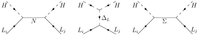
Figure 3.1: The three types of seesaw model - The three mediator fields that can produce the Weinberg Operator at low energies are the fermion singlet ($N$), the scalar triplet ($\Delta_{L}$) and the fermion triplet ($\Sigma$). In this figure $L$ stands for the lepton doublets $\ell_{L}$.

Here we will select the type I seesaw model which introduces right-handed neutrinos in analogy with the rest of fermions. These particles are perfect singlets under the Standard Model, see table 3.3, something that allows for their Majorana character which is transmitted to the left-handed neutrinos detected in experiment through the Yukawa couplings.

	$SU(3)_{c}$	$SU(2)_{L}$	$U(1)_{Y}$
$N_{R}$	1	1	0

Table 3.3: Right-handed neutrino charges under the SM group

The complete Lagrangian for the fermion masses is therefore:

$$\mathscr{L}_{fermion-mass}=\mathscr{L}_{Yukawa}+\mathscr{L}_{Majorana}\,,$$ (3.25)

$$\mathscr{L}_{Yukawa}= -\overline{Q}_{L}Y_{U}\tilde{H}U_{R}-\overline{Q}_{L}Y_{D}HD_{R}-\overline{\ell}_{L}Y_{E}E_{R}H-\overline{\ell}_{L}Y_{\nu}\tilde{H}N_{R}+h.c.\,,$$ (3.26)

$$\mathscr{L}_{Majorana}= -\overline{N}_{R}^{c}\frac{M}{2}N_{R}+h.c.\,,$$ (3.27)

where $M$ is a symmetric $3\times 3$ matrix and $N_{R}$ stands for the right-handed neutrinos which now also enter the sum of kinetic terms of Eq. 3.7. The limit in which the right-handed neutrino scale $M$ is much larger than the Dirac scale $Y_{\nu}v$ yields as first correction after integration of the heavy degrees of freedom the Weinberg Operator with the constants $c_{\alpha\beta}$ in Eq. 3.24 being $c_{\alpha\beta}=(Y_{\nu}Y_{\nu}^{T})_{\alpha\beta}/2$.

3.2.2 The Flavour Symmetry

If the gauge part was described around the gauge group one can do the same, if only formally a priori, for the flavour side. A way to characterize it is then choosing the largest symmetry that the free theory could present given the particle content and orthogonal to the gauge group, this symmetry is that of the group (23, 26, 27):

$$\qquad\qquad\qquad\qquad\qquad\mathcal{G_{F}}=\mathcal{G}_{\mathcal{F}}^{q}\times\mathcal{G}_{\mathcal{F}}^{l}\,,$$

$$\mathcal{G}_{\mathcal{F}}^{q}= SU(3)_{Q_{L}}\times SU(3)_{U_{R}}\times SU(3)_{D_{R}}\times U(1)_{B}\times U(1)_{A^{U}}\times U(1)_{A^{D}}\,,$$ (3.28)

$$\mathcal{G}_{\mathcal{F}}^{l}= SU(3)_{\ell_{L}}\times SU(3)_{E_{R}}\times O(3)_{N}\times U(1)_{L}\times U(1)_{A^{l}}\,,$$ (3.29)

It is clear that each $SU(3)$ factor corresponds to the different gauge representation fields which do not acquire mass in the absence of interactions. Right-handed neutrinos have however a mass not arising from interactions, but present already in the free Hamiltonian. Given this fact the largest symmetry possible in this sector is $O(3)$ for the degenerate case:

$$M=|M|I_{3\times 3}\,,$$ (3.30)

which is imposed here. The symmetry selected here can alternatively be defined as that arising, for the right-handed neutrino mass matrix of the above form, in the limit $\mathscr{L}_{Yukawa}\rightarrow 0$.

There is an ambiguity in the definition of the lepton sector symmetry and indeed other definitions are present in the literature (28, 29), in particular for the $N_{R}$ fields a $U(3)_{N_{R}}$ symmetry is selected if the symmetry is identified with the kinetic term of the matter fields. This option leads to a complete parallelism from the symmetry point of view for leptons and quarks and would consequently lead to similar outcomes in an unsuccessful scenario (18).

Under the non-abelian part of $\mathcal{G_{F}}$ the matter fields transform as detailed in table 3.4 and the abelian charges are given in table 3.5. In the non-abelian side one can identify $U(1)_{B}$ as the symmetry that preserves baryon number and $U(1)_{L}$ as lepton number which is broken in the full theory here considered. The remaining $U(1)_{A}$ symmetries are axial rotations in the quark and lepton sectors.

	$SU(3)_{Q_{L}}$	$SU(3)_{U_{R}}$	$SU(3)_{D_{R}}$	$SU(3)_{\ell_{L}}$	$SU(3)_{E_{R}}$	$O(3)_{N_{R}}$
$Q_{L}$	3	1	1	1	1	1
$U_{R}$	1	3	1	1	1	1
$D_{R}$	1	1	3	1	1	1
$\ell_{L}$	1	1	1	3	1	1
$E_{R}$	1	1	1	1	3	1
$N_{R}$	1	1	1	1	1	3

Table 3.4: Representation of the fermion fields under the non-abelian part of $\mathcal{G_{F}}$

	$U(1)_{B}$	$U(1)_{A^{U}}$	$U(1)_{A^{D}}$	$U(1)_{L}$	$U(1)_{A^{l}}$
$Q_{L}$	1/3	1	1	0	0
$U_{R}$	1/3	-1	0	0	0
$D_{R}$	1/3	0	-1	0	0
$\ell_{L}$	0	0	0	1	1
$E_{R}$	0	0	0	1	-1
$N_{R}$	0	0	0	0	0

Table 3.5: Representation of the fermion fields under the abelian part of $\mathcal{G_{F}}$

$\mathscr{L}_{Yukawa}$ is however non vanishing and encodes the flavour structure, our present knowledge about it being displayed in Eqs. 3.31-3.46. The masses for fermions range at least 12 orders of magnitude and the neutrinos are a factor $10^{6}$ lightest than the lightest charged fermion, something perhaps connected to their possible Majorana nature. Neutrino masses are not fully determined, only the two mass squared differences and and upper bound on the overall scale are known. The fact that one of the mass differences is only known in absolute value implies that not even the hierarchy is known, the possibilities being Normal Hierarchy (NH) $m_{\nu_{1}}<m_{\nu_{2}}<m_{\nu_{3}}$ and Inverted Hierarchy (IH) $m_{\nu_{3}}<m_{\nu_{1}}<m_{\nu_{2}}$.

The mixing shape for quarks is close to an identity matrix, with deviations given by the Cabibbo angle $\lambda_{c}$, whereas mixing angles are large in the lepton sector corresponding to all entries of the same order of magnitude in the mixing matrix. In the lepton sector the CP phase $\delta$ and the Majorana phases, if present, are yet undetermined. Altogether, our present knowledge of the flavour structure is encoded in the following data,

$$m_{d} =4.8^{+0.7}_{-0.3}\,\mbox{MeV}\,, m_{s} =95\pm 5\,\mbox{MeV}\,, m_{b} =4.18\pm 0.03\,\mbox{GeV}\,,$$ (3.31)

$$m_{u} =2.3^{+0.7}_{-0.5}\,\mbox{MeV}\,, m_{c} =1.275\pm 0.025\,\mbox{GeV}\,, m_{t} =173.5\pm 0.8\,\mbox{GeV}\,,$$ (3.32)

$$m_{e} =0.510998928\pm 0.000000011\,\mbox{MeV}\,,$$ (3.33)

$$m_{\mu} =105.6583715\pm 0.0000035\,\mbox{MeV}\,,$$ (3.34)

$$m_{\tau} =1.776.82\pm 0.16\,\mbox{GeV}\,,$$ (3.35)

$$\sum_{i}m_{\nu_{i}} \leq 0.28\,\mbox{eV}\,, \Delta m_{\nu_{12}}^{2} =7.5^{+0.2}_{-0.2}10^{-5}\,\mbox{eV}^{2}\,, |\Delta m_{\nu_{23}}^{2}| =2.42^{+0.04}_{-0.07}10^{-3}\,\mbox{eV}^{2}\,,$$ (3.36)

$$V_{CKM}=\left(\begin{array}[]{ccc}1-\lambda_{c}^{2}/2&\lambda_{c}&A\lambda_{c}^{3}\left(\rho-i\eta\right)\\ -\lambda_{c}&1-\lambda_{c}^{2}/2&A\lambda_{c}^{2}\\ A\lambda_{c}^{3}\left(1-\rho-i\eta\right)&-A\lambda_{c}^{2}&1\\ \end{array}\right)+\mathcal{O}(\lambda_{c}^{4})$$ (3.39)

$$A\lambda_{c}^{3}\left(\rho+i\eta\right)\equiv\frac{A\lambda_{c}^{3}\left(\bar{\rho}+i\bar{\eta}\right)\sqrt{1-A^{2}\lambda_{c}^{4}}}{\sqrt{1-\lambda_{c}^{2}}\left(1-A^{2}\lambda_{c}^{4}(\bar{\rho}+i\bar{\eta})\right)}\,,\qquad\lambda_{c}=0.22535\pm 0.00065\,,$$ (3.40)

$$A=0.811^{+0.022}_{-0.012}\,,\qquad\bar{\rho}=0.131^{+0.026}_{-0.013}\,,\qquad\bar{\eta}=0.345^{+0.013}_{-0.014}\,,$$ (3.41)

$$U_{PMNS}=\left(\begin{array}[]{ccc}c_{12}c_{13}&s_{12}c_{13}&s_{13}e^{-i\delta}\\ -s_{12}c_{23}-c_{12}s_{23}s_{13}e^{i\delta}&c_{12}c_{23}-s_{12}s_{23}s_{13}e^{i\delta}&s_{23}c_{13}\\ s_{12}s_{23}-c_{12}c_{23}s_{13}e^{i\delta}&-c_{12}s_{23}-s_{12}c_{23}s_{13}e^{i\delta}&c_{23}c_{13}\\ \end{array}\right)e^{i\alpha_{1}\lambda_{3}+i\alpha_{2}\lambda_{8}}\,,$$ (3.45)

$$\theta_{12}=33^{+0.88}_{-0.78}\,{}^{\circ}\qquad\theta_{23}=40-50\,^{\circ}\qquad\theta_{13}=8,66^{+0.44}_{-0.46}\,{}^{\circ}\,,$$ (3.46)

where the quark data is taken from (53), the neutrino parameters from (54, 55), Majorana phases $\alpha_{1}$ and $\alpha_{2}$, are encoded in the exponentials of the Gell-Mann matrices of Eq. 3.46, and $\Delta m_{\nu_{ij}}^{2}=m_{\nu_{j}}^{2}-m_{\nu_{i}}^{2}$.

The question arises of what becomes of the anomaly cancellation conditions now that the flavour structure has been made explicit. The conditions are still fixing the relative hypercharges of all generations provided all masses are different, all mixing angles nontrivial and Majorana masses for the right-handed neutrinos.

Comparison of the flavour and gauge sector will be useful for the introduction of the research subject of this thesis. First, the ratio of certain parameters of the gauge sector, namely hypercharges, cannot take arbitrary values but are fixed due to constraints for the consistency of the theory, while the values for the flavour parameters seem all to be equally valid, at least from the point of view of consistency and stability. This brings to a second point, the inputs that are arbitrary in the gauge sector, $g_{s},g,g^{\prime},\lambda$ are smaller but of $\mathcal{O}(1)$ at the typical scale of the theory $\sim M_{Z}$, whereas masses span over $6$ orders of magnitude for charged leptons and including neutrinos the orders of magnitude escalate to $12$.

Because of gauge invariance particles are fitted into representations of the group, such that the dimension of the representation dictates the number of particles. There are left-handed charged leptons and left-handed neutrinos to fit a fundamental representation of $SU(2)_{L}$, could it be that something alike happens in the flavour sector? That is, is there a symmetry behind the flavour structure?

If this is the case, the symmetry that dictates the representation is not evident at the scale we are familiar with, so it should somehow be hidden; we can tell an electron from a muon because they have different masses. But the very same thing happens for $SU(2)_{L}$, we can tell the neutrino from the electron as the electroweak symmetry is broken.

This comparison led neatly to the study carried out. We shall assume that there is an exact symmetry behind the flavour structure, and if so necessarily broken at low energies; a breaking that we will effectively describe via a flavour Higgs mechanism. It is the purpose of this dissertation to study the mechanism responsible for the breaking of such flavour symmetry in the search for a deeper explanation of the flavour structure of elementary particles.

4 Flavour Physics

4.1 Flavour in the Standard Model $+$ type I Seesaw Model

The model that serves as starting point in our discussion is the Standard Model with the addition of the type I seesaw model to account for neutrino masses, the widely accepted as simplest and most natural extension with lepton number violation. This chapter will be concerned with flavour phenomenology and the way it shapes the flavour structure of new physics at the TeV scale, aiming at the understanding from a bottom up approach of the sources of flavour violation. The way in which the flavour symmetry is violated in the theory here considered is indeed quite specific and yields sharp experimental predictions that we shall examine next.

The energies considered in this chapter are below the electroweak scale, such that the Lagrangian of Eq.  3.25, assuming $M\gg v$, after integrating out the heavy right-handed neutrinos reads

$$\mathscr{L}_{fermion-mass}= -\overline{Q}_{L}Y_{U}\tilde{H}U_{R}-\overline{Q}_{L}Y_{D}HD_{R}+h.c.$$

$$-\overline{\ell}_{L}Y_{E}E_{R}H-\overline{\ell}_{L}\tilde{H}\frac{Y_{\nu}Y_{\nu}^{T}}{2M}\tilde{H}^{T}\ell^{c}_{L}+h.c.+\mathcal{O}\left(\frac{1}{M^{2}}\right)$$ (4.1)

where we recall that the flavour symmetry here considered sets $M_{ij}=M\delta_{ij}$, a case that shall not obscure the general low energy characteristics of a type I seesaw model whereas it simplifies the discussion. The flavour symmetry in this model is only broken by the above Lagrangian, including $1/M^{n}$ corrections. In full generality the Yukawa matrices can be written as the product of a unitary matrix, a diagonal matrix of eigenvalues and a different unitary matrix on the right end. In the case of the light neutrino mass term, it is more useful to consider the whole product $Y_{\nu}Y_{\nu}^{T}$ which is a transpose general matrix and therefore decomposable in a unitary matrix and a diagonal matrix. Explicitly, this parametrization for the Yukawa couplings reads:

$$Y_{U} =\mathcal{U}^{U}_{L}\mathbf{y}_{U}\,\mathcal{U}^{U}_{R}\,, Y_{D} =\mathcal{U}^{D}_{L}\mathbf{y}_{D}\,\mathcal{U}^{D}_{R}\,,$$ (4.2)

$$Y_{E} =\mathcal{U}^{E}_{L}\mathbf{y}_{E}\,\mathcal{U}^{E}_{R}\,, Y_{\nu}Y_{\nu}^{T} =\mathcal{U}^{\nu}_{L}\hat{\mathbf{y}}_{\nu}^{2}\,\mathcal{U}^{\nu T}_{L}\,,$$ (4.3)

where $\mathcal{U}^{U,D,E,\nu}_{L,R}$ are the unitary matrices and $\mathbf{y}_{U,D,E}$ and $\hat{\mathbf{y}}_{\nu}$ the diagonal matrices containing the eigenvalues of charged fermion Yukawa matrices and $Y_{\nu}Y_{\nu}^{T}$ respectively. Even if the symmetry is broken, the rest of the SM and type I seesaw Lagrangian stays invariant under a transformation under the group $\mathcal{G_{F}}$ of the fermion fields. In particular the rotations:

$$Q_{L} \rightarrow\mathcal{U}_{L}^{D}Q_{L}\,, D_{R} \rightarrow\mathcal{U}_{R}^{D\dagger}D_{R}\,, U_{R} =\mathcal{U}^{R\dagger}_{R}U_{R}\,,$$ (4.4)

$$\ell_{L} \rightarrow\mathcal{U}_{L}^{E}\ell_{L}\,, E_{R} \rightarrow\mathcal{U}_{R}^{E\dagger}E_{R}\,,$$ (4.5)

simplify the Yukawa matrices in Eqs. 4.2,4.3 after substitution in Eq. 4.1 to,

$$Y_{U} =\mathcal{U}^{D\dagger}_{L}\,\mathcal{U}^{U}_{L}\mathbf{y}_{U}\,, Y_{D} =\mathbf{y}_{D}\,,$$ (4.6)

$$Y_{E} =\mathbf{y}_{E}\,, Y_{\nu}Y_{\nu}^{T} =\mathcal{U}^{E\dagger}_{L}\mathcal{U}^{\nu}_{L}\,\hat{\mathbf{y}}_{\nu}^{2}\,\mathcal{U}^{\nu T}_{L}\mathcal{U}^{E*}_{L}\,,$$ (4.7)

which allows to define:

$$V_{CKM}^{\dagger} \equiv\mathcal{U}^{D\dagger}_{L}\,\mathcal{U}^{U}_{L}\,, U_{PMNS} \equiv\mathcal{U}^{E\dagger}_{L}\mathcal{U}^{\nu}_{L}\,,$$ (4.8)

$$\mathbf{y}_{U} =\mbox{Diag}\left(y_{u},y_{c},y_{t}\right)\,, \mathbf{y}_{D} =\mbox{Diag}\left(y_{d},y_{s},y_{b}\right)\,,$$ (4.9)

$$\hat{\mathbf{y}}_{\nu} =\mbox{Diag}\left(\hat{y}_{\nu_{1}},\hat{y}_{\nu_{2}},\hat{y}_{\nu_{3}}\right)\,, \mathbf{y}_{E} =\mbox{Diag}\left(y_{e},y_{\mu},y_{\tau}\right)\,,$$ (4.10)

with $V_{CKM}$ being the usual quark mixing matrix and $U_{PMNS}$ the analogous in the lepton side; the first encodes three angles and one CP-odd phase and the second two extra complex Majorana phases on top the the equivalent of the previous 4 parameters. The connection of the eigenvalues with masses will be made clear below.

There are a few things to note here. The right handed unitary matrices $\mathcal{U}_{R}^{U,D,E}$ are irrelevant, the appearance of the irreducible mixing matrix in both sectors is due to the simultaneous presence of a Yukawa term for both up and down-type quarks involving the same quark doublet $Q_{L}$, and the neutrino mass term and charged lepton Yukawa where the lepton doublet $\ell_{L}$ appears. Were the mass terms to commute there would be no mixing matrix. Were the weak isospin group not present to bind together $u_{L}$ with $d_{L}$ and $\nu_{L}$ with $e_{L}$ there would not either be mixing matrix. Weak interactions in conjunction with mass terms violate flavour. Although mixing matrices are there and nontrivial it is useful to have in mind these considerations to remember how they arise.

After EWSB the independent rotation of the two upper components of the weak isospin doublets,

$$U_{L} \rightarrow V_{CKM}^{\dagger}\,U_{L}\,, \nu_{L} \rightarrow U_{PMNS}\,\nu_{L}\,,$$ (4.11)

takes to the mass basis yielding the Yukawa couplings diagonal,

$$\mathscr{L}_{fermion-mass}= -\frac{y_{\alpha}\,\left(v+h\right)}{\sqrt{2}}\,\overline{U}_{L}^{\alpha}U_{R}^{\alpha}-\frac{y_{i}\,\left(v+h\right)}{\sqrt{2}}\,\overline{D}_{L}^{i}D_{R}^{i}$$ (4.12)

$$-\frac{y_{\beta}\left(v+h\right)}{\sqrt{2}}\,\overline{E}_{L}^{\beta}E_{R}^{\beta}-\frac{\hat{y}_{\nu_{j}}^{2}\left(v+h\right)^{2}}{4M}\,\overline{\nu}_{L}^{j}\nu_{L}^{c\,,j}+h.c.\,,$$ (4.13)

were $h$ is the physical Higgs boson, the unitary gauge has been chosen and hereby greek indices run over up-type quark and charged lepton mass states and latin indixes over down-type quark and neutrino mass states, see Eqs. 4.9,4.10.

We read from the above that the masses for the charged fermions are $m_{\alpha}=y_{\alpha}v/\sqrt{2}=y_{\alpha}\times 174$GeV whereas for neutrinos $m_{\nu_{i}}=\hat{y}_{\nu_{i}}^{2}v^{2}/(2M)$. The values of masses then fix the Yukawa eigenvalues for the charged fermions to be:

$$\left\{y_{t}\,,\,y_{c}\,,\,y_{u}\right\}= \,\left\{1.0\,,\,7.3\times 10^{-3}\,,\,1.3\times 10^{-5}\right\}\,,$$ (4.14)

$$\left\{y_{b}\,,\,y_{s}\,,\,y_{d}\right\}= \,\left\{2.4\times 10^{-2}\,,\,5.5\times 10^{-4}\,,\,2.7\times 10^{-5}\right\}\,,$$ (4.15)

$$\left\{y_{\tau}\,,\,y_{\mu}\,,\,y_{e}\right\}= \,\left\{1.0\times 10^{-2}\,,6.0\times 10^{-4}\,,\,2.9\times 10^{-6}\right\}\,,$$ (4.16)

whereas for neutrinos only the mass squared differences are know and the upper bound of Eq. 3.36 sets $\hat{y}_{\nu}^{2}v^{2}/M\lesssim$ eV. The values for the Yukawa eigenvalues of the charged fermions display quantitatively the hierarchies in the flavour sector since, as dimensionless couplings of the theory, they are naturally expected of $\mathcal{O}(1)$, something only satisfied by the top Yukawa. The smallness of the eigenvalues is nonetheless stable under corrections since in the limit of vanishing Yukawa eigenvalue a chiral symmetry arises, which differentiates this fine-tuning from the Hierarchy Problem.

The rest of the Lagrangian does not notice the rotation in Eq. 4.11 except for the couplings of weak isospin $+1/2$ and $-1/2$ particles:

$$\mathscr{L}_{CC}=i\frac{g}{\sqrt{2}}\overline{U}_{L}V_{CKM}\not{W}^{+}D_{L}+i\frac{g}{\sqrt{2}}\overline{\nu}_{L}U_{PMNS}^{\dagger}\not{W}^{+}E_{L}+h.c.\,.$$ (4.17)

The rest of couplings, which involve neutral gauge bosons, are diagonal in flavour, to order $1/M^{2}$. The flavour changing source has shifted therefore in the mass basis to the couplings of fermions to the $W^{\pm}$ gauge bosons. This is in accordance with the statement of the need of both weak isospin and mass terms for flavour violation.

This process allows to give a physical definition of the unitary matrices entering the Yukawa couplings: mixing matrices parametrize the change of basis from the interaction to the mass basis. This is a more general statement than the explicit writing of Yukawa terms or the specification of the character of neutrino masses.

The absence of flavour violation in neutral currents implies the well known and elegant explanation of the smallness of flavour changing neutral currents (FCNC) of the Glashow-Iliopoulos-Maiani (GIM) mechanism (57). All neutral current flavour processes are loop level induced and suppressed by unitarity relations to be proportional to mass differences and mixing parameters, an achievement of the standard theory that helped greatly to its consolidation. At the same time this smallness of flavour changing neutral currents stands as a fire proof for theories that intend to extend the Standard Model, as we shall see next.

4.2 Flavour Beyond the Standard Model

The flavour pattern of elementary particles has been approached in a number of theoretical frameworks aiming at its explanation. Shedding light in a problem as involved as the flavour puzzle has proven not an easy task. Proposed explanations are in general partial, in particular reconciling neutrino flavour data with quark and charged lepton hierarchies in a convincing common framework is a pending task in the authors view.

In the following a number of the proposed answers to explain flavour are listed,

• Froggat -Nielsen theories. The introduction of an abelian symmetry $R$ under which the different generation fermions with different chirality have different charges and that is broken by the vev of a field $\left\langle\phi_{0}\right\rangle$ can explain the hierarchies in the flavour pattern (20). In this set-up there are extra chiral fermions at a high scale with a typical mass $\Lambda_{f}$ such that the magnitude $\epsilon=\left\langle\phi_{0}\right\rangle/\Lambda_{f}$ controls the breaking of the abelian symmetry $R$. Interactions among the different fermions are mediated by the field $\phi_{0}$ at the high scale and its acquisition of a vev at the low scale implies factors of $\epsilon^{a_{i}+b_{j}}$ for the coupling of different flavour and chirality fermions $\Psi_{L_{i}}$, $\Psi_{R_{j}}$ with charges $R_{L_{i}}=b_{i}$ and $R_{R_{j}}=-a_{j}$ normalized to the charge of $\phi_{0}$ ($R_{\phi_{0}}=1$). The mass matrix produced in this way contains hierarchies among masses controlled by $m_{i}/m_{j}\sim\epsilon^{a_{i}-a_{j}+b_{i}-b_{j}}$ whereas angles are given by $U_{ij}\sim(m_{i}/m_{j})^{C_{ij}}\gtrsim(m_{i}/m_{j})$. This symmetry based argument stands as one of the simplest and most illuminating approaches to the flavour puzzle.

• Discrete symmetries discrete symmetries were studied as possible explanations for the flavour pattern in the quark sector, e.g. (58), but the main focus today is on the lepton mixing pattern. The values of the atmospheric and solar angles motivated proposals of values for the angles given by simple integer ratios like the tri-bimaximal mixing pattern (59) ($\theta_{23}=\pi/4\,,\,\theta_{12}=$arcsin$(1/\sqrt{3})\,,\,\theta_{13}=0$) . These patterns were later shown to be obtainable with breaking patterns of relatively natural discrete symmetries like $A_{4}$(60, 61, 62) or $S_{4}$ (63, 64). A discrete flavour treatment of both quarks and leptons requires generally of extra assumptions like distinct breaking patterns in distinct fermion sectors which have to be kept separate, see e.g. (65, 66). These models though are now in tension with the relatively large reactor angle and new approaches are being pursued (67, 68). This approach has the advantage of avoiding Goldstone bosons when breaking the discrete symmetry but the drawback of the ambiguity in choosing the group.

• Extra Dimensions The case of extra dimension offers a different explanation for the hierarchy in masses. In Randall-Sundrum models (69, 70) the presence of two 4d branes in a 5 dimensional space induces a metric with an overall normalization or warp factor that is exponentially decreasing with the fifth dimension and that offers an explanation of the huge hierarchy among the Planck and EW scale in terms of $\mathcal{O}(1)$ fundamental parameters. When the fermions are allowed to propagate in the fifth dimension, rather than being confined in a brane, their profile in the fifth dimension determined by the warp factor and a bulk mass term provides exponential factors for the Yukawa couplings as well, offering an explanation of the flavour pattern in terms of $\mathcal{O}(1)$ fundamental or 5th dimensional parameters (71, 72). In large extra dimensions theories, submilimiter new spacial directions can provide geometrical factors to explain the hierarchy problem (73). In this scenario, if we live on a “fat” brane in which the fermion profiles are localized, the mixing among generations is suppressed by the overlap of this profiles rather than symmetry arguments (74, 75, 76). In the extradimensional paradigm in general therefore the explanation of the hierarchies in flavour is found in geometry rather than symmetry.

• Anarchy The possibility of the flavour parameters being just random numbers without any utter reason has been also explored (77, 78), and even if the recent measurement of a “large” $\theta_{13}$ lepton mixing angle favors this hypothesis for the neutrino mass matrix (79), the strongly hierarchical pattern of masses and mixing of charged fermions is not natural in this framework.

These models introduce in general new physics coupled to the flavour sector of the Standard Model, which means modifying the phenomenological pattern too. This observation applies to other models as well: any new physics that couples to the SM flavour sector will change the predictions for observables and shall be contrasted with data. This is examined next.

4.3 Flavour Phenomenology

Once again the effective field theory is put to use,

$$\mathscr{L}=\mathscr{L}_{SM}+\frac{1}{M}\mathcal{O}^{W}+\sum\frac{c_{i}}{\Lambda_{f}^{2}}\mathcal{O}^{i}+\mathcal{O}(1/\Lambda_{f}^{3})$$ (4.18)

This Lagrangian describes the Standard Model theory, represented by the first term, plus new physics corrections in a very general manner encoded in the two next terms. The first correction in Eq. 4.18 is the Weinberg Operator of Eq. 3.24 which has already been examined and taken into account. The next corrections have a different scale $\Lambda_{f}$ motivated by naturalness criteria. In this category we include the operators that do not break lepton number nor baryon number, listed in (80) and only recently reduced to the minimum set via equations of motion (81). Therefore they need not be suppressed by the lepton number violation scale $M$. There are nonetheless contributions of $1/M^{2}$ in Eq. 4.18, but these are too small for phenomenological purposes after applying the upper bound from neutrino masses. Let us note that in certain seesaw models the lepton number and flavour scales are separated (82, 83, 84, 85, 86), such that their low energy phenomenology falls in the description above (87, 88). As a concrete example of a modification to the SM a possible operator at order $1/\Lambda_{f}^{2}$ is:

$$c_{6}\,\mathcal{O}^{6}=c_{\alpha\beta\sigma\rho}\bar{Q}_{L}^{\alpha}\gamma_{\mu}Q_{L}^{\beta}\bar{Q}_{L}^{\sigma}\gamma^{\mu}Q_{L}^{\rho}\,,$$ (4.19)

where greek indices run over different flavours and the constants $c_{\alpha\beta\sigma\rho}$ are the coefficients different in general for each flavour combination.

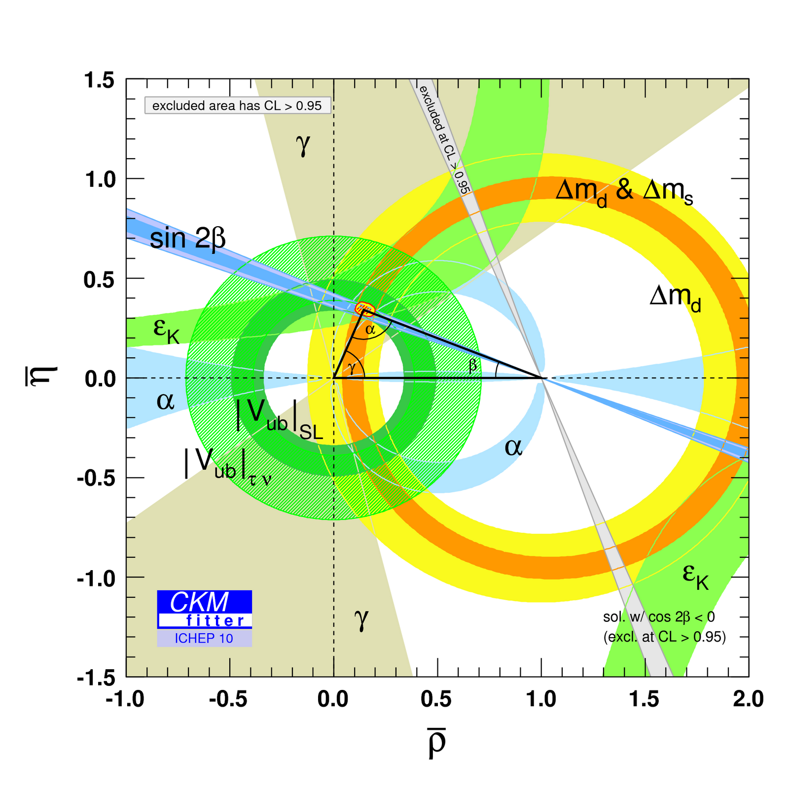
Figure 4.1: Experimentally allowed regions for the CKM mixing parameters $\bar{\rho}$ and $\bar{\eta}$ - The overlap of the experimentally allowed regions extracted from kaon and B-meson observables in the $\bar{\rho}-\bar{\eta}$ plane, mixing parameters defined in Eq. 3.41, shows the good agreement of the SM with the flavour data.

The modification induced by this term in observable quantities can be computed and compared with data. A wide and ambitious set of experiments has provided the rich present amount of flavour data; from the precise branching ratios of B mesons in B factories to the search for flavour violation in the charged lepton sector, all the D and K meson observables, and if we include CP violation, the stringent electric dipole moments.

Contrast of the experimental data with expectations has led, in most occasions, to a corroboration of the Standard Model in spite of new physics, and at times certain hints of deviations from the standard theory raised hopes (a partial list is (89, 90, 91)) that either were washed away afterwards, or stand as of today inconclusive. It is the case then that no clear proof of physics other than the SM and neutrino masses driving flavour data has been found.

Indeed the data has been not only enough to determine the flavour parameters of the SM but also to impose stress tests on the theory, all faintlessly passed. Fig. 4.1 shows how all experimentally allowed regions in the mixing parameter plane of $\bar{\rho}-\bar{\eta}$, variables defined in Eq. 3.41, meet around the allowed value.

Operator	Bounds on $\Lambda_{f}$ (TeV)	Bounds on $c$ ($\Lambda_{f}=1$TeV)	Observables
	$c=1$                $c=i$	$\mathfrak{Re}(c)$                 $\mathfrak{Im}(c)$
$\left(s_{L}\gamma_{\mu}d_{L}\right)^{2}$	$9.8\times 10^{2}\,\,\,\,\,\,1.6\times 10^{4}$	$9.0\times 10^{-7}\,\,\,\,\,\,3.4\times 10^{-9}$	$\Delta m_{K},\epsilon_{K}$
$(s_{R}d_{L})(s_{L}d_{R})$	$1.8\times 10^{4}\,\,\,\,\,\,3.2\times 10^{5}$	$6.9\times 10^{-9}\,\,\,\,\,\,2.6\times 10^{-11}$	$\Delta m_{K},\epsilon_{K}$
$(c_{L}\gamma_{\mu}u_{L})^{2}$	$1.2\times 10^{3}\,\,\,\,\,\,2.9\times 10^{3}$	$5.6\times 10^{-7}\,\,\,\,\,\,1.0\times 10^{-7}$	$\Delta m_{D};|q/p|;\phi_{D}$
$(c_{R}u_{L})(c_{L}u_{R})$	$6.2\times 10^{3}\,\,\,\,\,\,1.5\times 10^{4}$	$5.7\times 10^{-8}\,\,\,\,\,\,1.1\times 10^{-8}$	$\Delta m_{D};|q/p|;\phi_{D}$
$(b_{L}\gamma_{\mu}d_{L})^{2}$	$6.6\times 10^{2}\,\,\,\,\,\,9.3\times 10^{2}$	$2.3\times 10^{-6}\,\,\,\,\,\,1.1\times 10^{-6}$	$\Delta m_{B_{d}};S_{\Psi K_{S}}$
$(b_{R}d_{L})(b_{L}d_{R})$	$2.5\times 10^{3}\,\,\,\,\,\,3.6\times 10^{3}$	$3.9\times 10^{-7}\,\,\,\,\,\,1.9\times 10^{-7}$	$\Delta m_{B_{d}};S_{\Psi K_{S}}$
$(b_{L}\gamma_{\mu}s_{L})^{2}$	$1.4\times 10^{2}\,\,\,\,\,\,2.5\times 10^{2}$	$5.0\times 10^{-5}\,\,\,\,\,\,1.7\times 10^{-5}$	$\Delta m_{B_{s}};S_{\Psi\Phi}$
$(b_{R}s_{L})(b_{L}s_{R})$	$4.8\times 10^{2}\,\,\,\,\,\,8.3\times 10^{2}$	$8.8\times 10^{-6}\,\,\,\,\,\,2.9\times 10^{-6}$	$\Delta m_{B_{s}};S_{\Psi\Phi}$
$F^{\mu\nu}\bar{\mu}_{R}\sigma_{\mu\nu}e_{L}$	$6.1\times 10^{4}\,\,\,\,\,\,6.1\times 10^{4}$	$2.7\times 10^{-10}\,\,\,\,\,\,2.7\times 10^{-10}$	$\mu\rightarrow e\gamma$
$(\mu_{L}\gamma_{\mu}e_{L})(u_{L}\gamma_{\mu}u_{L})$	$4.9\times 10^{2}\,\,\,\,\,\,4.9\times 10^{2}$	$4.1\times 10^{-6}\,\,\,\,\,\,4.1\times 10^{-6}$	$\mu\rightarrow e(Ti)$
$(\mu_{L}\gamma_{\mu}e_{L})(d_{L}\gamma_{\mu}d_{L})$	$5.4\times 10^{2}\,\,\,\,\,\,5.4\times 10^{2}$	$3.5\times 10^{-6}\,\,\,\,\,\,3.5\times 10^{-6}$	$\mu\rightarrow e(Ti)$

Table 4.1: Bounds on the different operators, see text for details.

The absence of new physics evidence translates in bounds on the new physics scale, reported in table 4.1. When placing the bounds, the magnitude that is constrained is the combination $c/\Lambda_{f}^{2}$ as is the one appearing in the Lagrangian of Eq. 4.18. Naturalness criteria points at constants $c$ of $\mathcal{O}(1)$, a case reported in table 4.1 both for CP conservation $c=1$ (second column) and CP violation $c=i$ (third column). On the other hand if the scale is fixed at the TeV then the constants have severe upper bounds as the fourth and fifth columns in table 4.1 show. The quark bounds are taken from (92) whereas the lepton data is taken from (93, 94) and computed with the formulae of (14).

4.4 Minimal Flavour Violation

The bounds on new physics place a dilemma: either giving up new physics till the thousands of TeVs scale and with it the possibility of any direct test in laboratories, or assume that the flavour structure of new physics is highly non-generic or fined-tuned.

A solution to this dichotomy is the celebrated Minimal Flavour Violation scheme (26, 27, 28, 29) which is predictive, realistic, model independent and symmetry driven. The previous section showed that flavour phenomenology at present is explained by the SM plus neutrino masses solely, this is to say that the mass terms contain all the known flavour structure and ergo determine the flavour violation. The conclusion is that the mass terms are the only source for all flavour and CP violation data at our disposal. The minimality assumption of MFV is to upgrade this source to be the only one in physics Beyond the Standard Model at low energies.

In the absence of the mass terms the theory presents a symmetry which is formally conserved if the sources of flavour violation are assigned transformation properties, given in table 4.2 for the present realization.

	$SU(3)_{Q_{L}}$	$SU(3)_{U_{R}}$	$SU(3)_{D_{R}}$	$SU(3)_{\ell_{L}}$	$SU(3)_{E_{R}}$	$O(3)_{N_{R}}$
$Y_{U}$	3	$\bar{3}$	1	1	1	1
$Y_{D}$	3	1	$\bar{3}$	1	1	1
$Y_{E}$	1	1	1	$3$	$\bar{3}$	1
$Y_{\nu}$	1	1	1	$3$	$1$	3

Table 4.2: Spurious transformations of the Yukawa couplings under $\mathcal{G}_{\mathcal{F}}$

The formal restoration of the flavour symmetry applied in the effective field theory set-up determines the flavour constants which shall be such as to form flavour invariant combinations with the matter fields and built out of the sole sources of flavour violation at low energies, the Yukawas. The previous operator will serve as example now:

$$c_{6}\,\mathcal{O}^{6}=\bar{Q}_{L}^{\alpha}\left(Y_{U}Y_{U}^{\dagger}\right)_{\alpha\beta}\gamma_{\mu}Q_{L}^{\beta}\bar{Q}_{L}^{\sigma}\left(Y_{U}Y_{U}^{\dagger}\right)_{\sigma\rho}\gamma^{\mu}Q_{L}^{\rho}\,.$$ (4.20)

where the transformations listed in Tables 3.4 , 4.2 leave the above construction invariant. The Yukawa couplings, can be written as in Eqs. 4.6 , 4.8 , 4.9 and therefore all parameters entering the example of Eq. 4.20 are known; they are just masses and mixings.

It should be underlined that MFV is not a model of flavour and the value of the new dynamical flavour scale $\Lambda_{f}$ is not fixed, however the suppression introduced via the flavour parameters makes this scale compatible with the TeV, see (95) for a recent analysis. What it does predict is precise and constrained relations between different flavour transitions.

5 Spontaneous Flavour Symmetry Breaking

The previous chapter illustrated how the entire body of flavour data can be explained through a single entity, the mass terms. This has been shown to be the only culprit of flavour violation. If we pause and look at the previous sentence, it is interesting to see how the jargon itself already assumes that there is something to be violated and implicitly a breaking idea. It has been shown that the symmetry of the matter content of the free theory here considered is the product of the gauge and flavour symmetries; $\mathcal{G}\times\mathcal{G_{F}}$, and that Yukawa terms do not respect $\mathcal{G_{F}}$. Subgroups of this group could also be considered, here the full $\mathcal{G_{F}}$ is adopted in the general case, although in certain cases the axial abelian factors $U(1)_{A}$ will be dropped. The case of conservation of the full $\mathcal{G_{F}}$ group is also denoted axial conserving case, whereas assuming that the $U(1)_{A}$ symmetries are not exact will constitute the explicitly axial breaking case $\mathcal{G}_{\mathcal{F}}^{\not{A}}\sim SU(3)^{5}\times SO(3)$. In all cases the full non-abelian group is considered.

The ansatz of MFV showed the usefulness of assigning spurious transformation properties to the Yukawa couplings and having a formal flavour conservation at the phenomenological level. It is only natural to take the next step and assume the flavour symmetry is exact at some high energy scale $\Lambda_{f}$ and the Yukawa couplings are the remains of fields that had real transformations properties under this symmetry. The underlying idea of dynamical Yukawa couplings is depicted in Fig. 5.1 which resembles similar diagrams in Froggat-Nielsen theories. The basic assumption is indeed already present in the literature; for example in the first formulation of MFV by Chivukula and Georgi (23), the Yukawa couplings corresponded to a fermion condensate. It should be mentioned that a flavour breaking mechanism with different continuos non-abelian groups than the here considered has been explored in the quark (19, 96, 97, 98, 25) and lepton (99, 100, 101) sectors, whereas the invariant pieces needed to construct a potential were made explicit and analyzed for quarks and the group $\mathcal{G}_{\mathcal{F}}^{q}$ in Refs. (102, 99, 100). The quantum corrections to the work of Ref. (15) were studied in Refs. (103, 104).

The analysis of a two generation case will serve as illustration and guide in the next chapter, for this reason it is useful and compact to introduce $n_{g}$ for the number of generations. The straight-forward generalization of the flavour group is then:

$$\qquad\qquad\qquad\qquad\qquad\qquad\mathcal{G_{F}}=\mathcal{G}_{\mathcal{F}}^{q}\times\mathcal{G}_{\mathcal{F}}^{l}\,,$$

$$\mathcal{G}_{\mathcal{F}}^{q}= SU(n_{g})_{Q_{L}}\times SU(n_{g})_{U_{R}}\times SU(n_{g})_{D_{R}}\times U(1)_{B}\times U(1)_{A^{U}}\times U(1)_{A^{D}}\,,$$ (5.1)

$$\mathcal{G}_{\mathcal{F}}^{l}= SU(n_{g})_{\ell_{L}}\times SU(n_{g})_{E_{R}}\times O(n_{g})_{N}\times U(1)_{L}\times U(1)_{A^{l}}\,.$$ (5.2)

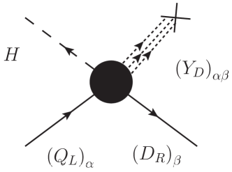
Figure 5.1: Yukawa Couplings as vevs of flavour fields -

5.1 Flavour Fields Representation

The starting point is rendering the Yukawa interaction explicitly invariant under the flavour symmetry. At the scale $\Lambda_{f}$ of the new fields responsible for flavour breaking, the Yukawa couplings will be dynamical themselves, implying the mass dimension of the Yukawa Operator is now $>4$.

Scalar Flavour Fields in the Bi-Fundamental

In the effective field theory expansion, the leading term is dimension 5:

$$\mathscr{L}_{Yukawa}=\overline{Q}_{L}\dfrac{\mathcal{Y}_{D}}{\Lambda_{f}}D_{R}H+\overline{Q}_{L}\dfrac{\mathcal{Y}_{U}}{\Lambda_{f}}U_{R}\tilde{H}+\overline{\ell}_{L}\dfrac{\mathcal{Y}_{E}}{\Lambda_{f}}E_{R}H+\overline{\ell}_{L}\dfrac{\mathcal{Y}_{\nu}}{\Lambda_{f}}N_{R}\tilde{H}+h.c.\,,$$ (5.3)

where there is the need to introduce the cut-off scale $\Lambda_{f}$, the scalar fields $\mathcal{Y}_{D}$, $\mathcal{Y}_{U}$, $\mathcal{Y}_{E}$ and $\mathcal{Y}_{\nu}$ are dynamical fields in the bi-fundamental representation as detailed in tables 5.1,5.2,

	$SU(n_{g})_{Q_{L}}$	$SU(n_{g})_{U_{R}}$	$SU(n_{g})_{D_{R}}$	$U(1)_{B}$	$U(1)_{A^{U}}$	$U(1)_{A^{D}}$
$\mathcal{Y}_{U}$	$n_{g}$	$\bar{n}_{g}$	1	0	2	1
$\mathcal{Y}_{D}$	$n_{g}$	1	$\bar{n}_{g}$	0	1	2

Table 5.1: $\mathcal{G}_{\mathcal{F}}^{q}$ representation of the quark sector bi-fundamental scalar fields for $n_{g}$ fermion generations

	$SU(n_{g})_{\ell_{L}}$	$SU(n_{g})_{E_{R}}$	$O(n_{g})_{N_{R}}$	$U(1)_{L}$	$U(1)_{A^{l}}$
$\mathcal{Y}_{E}$	$n_{g}$	$\bar{n}_{g}$	1	0	2
$\mathcal{Y}_{\nu}$	$n_{g}$	1	$n_{g}$	1	1

Table 5.2: $\mathcal{G}_{\mathcal{F}}^{l}$ representation of the lepton sector bi-fundamental scalar fields for $n_{g}$ fermion generations

and the relation to ordinary Yukawas is:

$$Y_{D}\equiv\dfrac{\left\langle\mathcal{Y}_{D}\right\rangle}{\Lambda_{f}}\,,\qquad\quad Y_{U}\equiv\dfrac{\left\langle\mathcal{Y}_{U}\right\rangle}{\Lambda_{f}}\,,\qquad\quad Y_{E}\equiv\dfrac{\left\langle\mathcal{Y}_{E}\right\rangle}{\Lambda_{f}}\,,\qquad\quad Y_{\nu}\equiv\dfrac{\left\langle\mathcal{Y}_{\nu}\right\rangle}{\Lambda_{f}}\,.$$ (5.4)

This case is hereby labeled bi-fundamental scenario, and the fields can be thought of as matrices whose explicit transformation is:

$$\mathcal{Y}_{U}(x) \xrightarrow{\mathcal{G_{F}}}\Omega_{Q_{L}}\mathcal{Y}_{U}(x)\,\Omega_{U_{R}}^{\dagger}\,, \mathcal{Y}_{D}(x) \xrightarrow{\mathcal{G_{F}}}\Omega_{Q_{L}}\mathcal{Y}_{D}(x)\,\Omega_{D_{R}}^{\dagger}\,,$$ (5.5)

$$\mathcal{Y}_{E}(x) \xrightarrow{\mathcal{G_{F}}}\Omega_{\ell_{L}}\mathcal{Y}_{E}(x)\,\Omega_{E_{R}}^{\dagger}\,, \mathcal{Y}_{\nu}(x) \xrightarrow{\mathcal{G_{F}}}\Omega_{\ell_{L}}\mathcal{Y}_{\nu}(x)\,O_{N_{R}}^{T}\,,$$ (5.6)

$\Omega_{\psi}$ ($O_{N_{R}}$) being a unitary (real orthogonal) matrix of the corresponding $\mathcal{G_{F}}$ subgroup: $\Omega_{\psi}\Omega_{\psi}^{\dagger}=\Omega_{\psi}^{\dagger}\Omega_{\psi}=1$, $\psi=Q_{L}\,...\,E_{R}$ ($O_{N_{R}}O_{N_{R}}^{T}=O_{N_{R}}^{T}O_{N_{R}}=1$).

Scalar Flavour Fields in the Fundamental

The next order in the effective field theory is a $d=6$ Yukawa operator, involving generically two scalar fields in the place of the Yukawa couplings,

$$\mathscr{L}_{Yukawa}=\overline{Q}_{L}\frac{\chi_{D}^{L}\chi_{D}^{R\dagger}}{\Lambda_{f}^{2}}D_{R}H+\overline{Q}_{L}\frac{\chi_{U}^{L}\chi_{U}^{R\dagger}}{\Lambda_{f}^{2}}U_{R}\tilde{H}+\overline{\ell}_{L}\frac{\chi_{E}^{L}\chi_{E}^{R\dagger}}{\Lambda_{f}^{2}}E_{R}H+\overline{\ell}_{L}\frac{\chi_{\nu}^{L}\chi_{\nu}^{R\dagger}}{\Lambda_{f}^{2}}N_{R}\tilde{H}\,,$$ (5.7)

which provide the following relations between Yukawa couplings and vevs:

$$Y_{D}\equiv\dfrac{\left\langle\chi_{D}^{L}\chi_{D}^{R\dagger}\right\rangle}{\Lambda_{f}^{2}}\,,\qquad Y_{U}\equiv\dfrac{\left\langle\chi_{U}^{L}\chi_{U}^{R\dagger}\right\rangle}{\Lambda_{f}^{2}}\,,\qquad Y_{E}\equiv\dfrac{\left\langle\chi_{E}^{L}\chi_{E}^{R\dagger}\right\rangle}{\Lambda_{f}^{2}}\,,\qquad Y_{\nu}\equiv\dfrac{\left\langle\chi_{\nu}^{L}\chi_{\nu}^{R\dagger}\right\rangle}{\Lambda_{f}^{2}}\,,\qquad$$ (5.8)

The simplest assignation of charges or transformation properties of these fields is to consider each of them in the fundamental representation of a given $SU(3)_{\psi}$ subgroup as specified in tables 5.3 , 5.4.

	$SU(n_{g})_{Q_{L}}$	$SU(n_{g})_{U_{R}}$	$SU(n_{g})_{D_{R}}$	$U(1)_{B}$	$U(1)_{A^{U}}$	$U(1)_{A^{D}}$
$\chi^{L}_{U}$	$n_{g}$	1	1	0	1	1
$\chi^{L}_{D}$	$n_{g}$	1	1	0	1	1
$\chi^{R}_{U}$	1	$n_{g}$	1	0	-1	0
$\chi^{R}_{D}$	1	1	$n_{g}$	0	0	-1

Table 5.3: Representation of the quark sector fundamental scalar fields for $n_{g}$ fermion generations

	$SU(n_{g})_{\ell_{L}}$	$SU(n_{g})_{E_{R}}$	$O(n_{g})_{N_{R}}$	$U(1)_{L}$	$U(1)_{A^{l}}$
$\chi^{L}_{E}$	$n_{g}$	1	1	0	1
$\chi^{L}_{\nu}$	$n_{g}$	1	1	0	1
$\chi^{R}_{E}$	1	$n_{g}$	1	0	-1
$\chi^{R}_{N}$	1	1	$n_{g}$	0	0

Table 5.4: Representation of the lepton sector fundamental scalar fields for $n_{g}$ fermion generations

These fields are then complex $n_{g}$-vectors whose transformation under the flavour group is just a unitary or real rotation; $\chi_{\psi}\xrightarrow{\mathcal{G_{F}}}\Omega_{\psi}\chi_{\psi}\,,\,\chi_{N}^{R}\xrightarrow{\mathcal{G_{F}}}O_{N_{R}}\chi_{N}^{R}$. From the group theory point of view this is the decomposition in the irreducible pieces needed to build up invariant Yukawa operators, and as we shall see their properties translate into an easy and clear extraction of the flavour structure.

The third case of a Yukawa operator of mass dimension 7 could arise from a condensate of fermionic fields $Y\sim\left\langle\overline{\Psi}\Psi\right\rangle/\Lambda_{f}^{3}$ (23), or as the product of three scalar fields. In both cases the simplest decomposition falls trivially into one of the previous or the assignation of representations is an otherwise unnecessarily complicated higher dimensional one.

Notice that realizations in which the Yukawa couplings correspond to the vev of an aggregate of fields, rather than to a single field, are not the simplest realization of MFV as defined in Ref. (26), while still corresponding to the essential idea that the Yukawa spurions may have a dynamical origin.

Finally, another option of dependence of the Yukawa couplings on the dynamical fields is an inverse one:

$$Y_{D}\equiv\dfrac{\Lambda_{f}}{\left\langle\mathcal{Y}_{D}\right\rangle}\,,\qquad Y_{U}\equiv\dfrac{\Lambda_{f}}{\left\langle\mathcal{Y}_{U}\right\rangle}\,,\qquad Y_{E}\equiv\dfrac{\Lambda_{f}}{\left\langle\mathcal{Y}_{E}\right\rangle}\,,\qquad Y_{\nu}\equiv\dfrac{\Lambda_{f}}{\left\langle\mathcal{Y}_{\nu}\right\rangle}\,.$$ (5.9)

a case in which the vev of the field rather than the scale $\Lambda_{f}$ entering the relation is the larger one. This interesting case arises in models of gauged flavour symmetry (105, 106, 107), in which the anomaly cancellation requirements call for the introduction of fermion fields, whose interaction in a renormalizable Lagrangian with the scalar fields and ordinary fermions suffice to constitute a self consistent theory that after the integration of the heavy states yields the relation above. The transformation properties of the fields are the same as in the bi-fundamental case.

For simplicity in the group decomposition and since they appear as the two leading terms in the effective field theory approach, we will focus the analysis here in the fundamental and bi-fundamental cases, or the dimension 5 and 6 Yukawa operators, the former nonetheless also applies to relation 5.9.

5.2 The Scalar Potential

The way in which the scalar fields $\mathcal{Y}\,,\,\chi$ acquire a vev is through a scalar potential. This potential must be invariant under the gauge group of the SM $\mathcal{G}$ and the flavour group $\mathcal{G_{F}}$. The study is focused on the potential constituted by the flavour fields only, even if there might be some mixing with the singlet combination $H^{\dagger}H$ of the Higgs field, an exploration of this last case can be found in (108) in which the flavour scalar fields are postulated as Dark Matter. Resuming, the coupling with the Higgs doublet would add to the hierarchy problem but make no difference in the determination of the flavour fields minimum since the mass scale of the latter is taken larger than the Higgs vev: $\Lambda_{f}^{2}\gg v^{2}$.

The goal of this work is therefore to address the problem of the determination and analysis of the general $\mathcal{G_{F}}$-invariant scalar potential and its minima for the flavour scalar fields denoted above by $\mathcal{Y}$ and $\chi$. The central question is whether it is possible to obtain the SM Yukawa pattern - i.e. the observed values of quark masses and mixings- with a “natural” potential.

It is worth noticing that the structure of the scalar potentials constructed here is more general than the particular effective realization in Eqs. 5.4 and 5.8 and it would apply also for Eq. 5.9 as it relies exclusively on invariance under the symmetry $\mathcal{G_{F}}$ and on the flavour field representation, bi-fundamental or fundamental.

This observation is relevant, because the case of gauged flavour symmetry leading to Eq. 5.9 addresses two problems that this approach has. Namely the presence of Goldstone bosons as a result of the spontaneous breaking of a continuous symmetry and the constraints placed on the presence of new particles carrying flavour and inducing potentially dangerous FCNC effects.

The Goldstone bosons in a spontaneously broken flavour gauge symmetry are eaten by the flavour group vector bosons which become massive. These particles even if massive would induce dangerous flavour changing processes which we expect to be suppressed by their scale. The case of gauged flavour symmetries is however such that the inverse relation of Yukawas of Eq. 5.9 translates also to the particle masses, so that the new particles inducing flavour changing in the lightest generations are the heaviest in the new physics spectrum (109). These two facts conform a possible acceptable and realistic scenario where to embed the present study.

5.2.1 Generalities on Minimization

The variables in which we will be minimizing are the parameters of the scalar fields modulo a $\mathcal{G_{F}}$ transformation. The discussion of which are those variables in the bi-fundamental case is familiar to the particle physicist: they are the equivalent of masses and mixing angles. Indeed we can substitute in Eq. 5.4 the explicit formula for the Yukawas, Eqs. 4.6 -4.10, and express the variables of the scalar field at the minimum in terms of flavour parameters.

The equation obtained in this way is the condition of the vev of the scalar fields fixing the masses and mixings that are measured. It is not clear at all though that a spontaneous breaking mechanism can yield the very values that Yukawas actually have. To find this out the minimization of the potential has to be completed, such that for the next two chapters masses and mixing will be treated as variables roaming all their possible range. The question is whether at the minimum of the potential these variables can take the values corresponding to the known spectrum and if so to which cost.

The $\mathcal{G_{F}}$ invariants, out of which the potential is built, will be denoted generically by $I_{j}$, while $y_{i}$ stand for the physical variables of the scalar fields connected explicitly to masses and mixing. Let us call $n$ the number of physical parameters that suffice to describe the general vev of the flavour fields, that is to say there are $n$ variables $y_{i}\,,i=1,2,...,n$.

A simple result is that there are $n$ independent invariants $I_{j}$, since the inversion of the relation of the latter in terms of the variables allows to express any new invariant $I^{\prime}$ in terms of the independent set $\{I_{j}\}$; $I^{\prime}=I^{\prime}(y_{i})=I^{\prime}(y_{i}(I_{j}))$.

In terms of the set of invariants $\{I_{j}\}$ the stationary or extremal points of the potential, among them the true vacuum, are the solutions to the equation,

$$\sum_{j}\frac{\partial I_{j}}{\partial y_{i}}\frac{\partial V}{\partial I_{j}}=0\,,$$ (5.10)

where $V$ stands for the general potential. These $n$ equations will fix the $n$ parameters. One can regard this array of equations as a matrix $J_{ij}=\partial I_{j}/\partial y_{i}$, which is just the Jacobian of the change of “coordinates” $I_{j}=I_{j}(y_{i})$, times a vector $\partial V/\partial I_{j}$.

This system, if the Jacobian has rank $n$, has only the solution of a null vector $\partial V/\partial I_{j}=0$, which is the case for example for the Higgs potential of the SM.

When the Jacobian has rank smaller than $n$, the system of Eqs. 5.10 simplifies to a number of equations equal to the rank of the Jacobian. The extreme case would be a rank 0 Jacobian, which is the trivial, but always present, symmetry preserving case. This link of the smallest rank with the largest symmetry can be extended; indeed in general terms the reduction of the rank implies the appearance of symmetries left unbroken. A conjectured theorem by Michel and Radicati (97, 96), translated to the notation used here, states that the maximal unbroken subgroup cases, given the fields that break the symmetry, are insured an stationary point when the values of the fields are confined to a compact region. N. Cabibbo and L. Maiani completed the study of an explicit example of the above theorem (19) while introducing the tool of the Jacobian analysis as it is used in this thesis together with a geometrical interpretation outlined next.

For a geometric comprehension of the reduction of the Jacobian’s rank the manifold of possible values for the invariants can be considered, hereby denoted $I$-manifold. The $I$-manifold can be embedded in a $n$-$th$ dimensional real space $\mathcal{R}^{n}$. Whenever the Jacobian has reduced rank there exist one or more directions in which a variation in the parameters $y$ has 0 variation in the I-manifold, let us denote this displacement $\delta y_{i}$, then this statement reads,

$$\delta I_{j}=\sum_{i}\frac{\partial I_{j}}{\partial y_{i}}\,\delta y_{i}=0\,.$$ (5.11)

This direction is the normal to a boundary of the $I$-manifold, as displacements in this direction are not allowed.The further the rank is reduced the more reduced is the dimension of this boundary. Those points for which the rank was reduced the most while still triggering symmetry breaking, will be denoted singular here; they are the maximal unbroken symmetry cases.

In the general case one can expect to have a combination of both, reduced rank of the Jacobian and potential-dependent solutions. In this sense the present study adds to the work of Refs. (19, 97, 96) two points through the study of an explicit general potential: i) we will be able to determine under what conditions the singular points (or maximal unbroken configurations) correspond to absolute minima; ii) the exploration of the general case will reveal whether other than singular minima are allowed or not. It is in any case worth examining first the Jacobian, as it is done in the next chapters.

Another relevant issue is the number of invariants that enter the potential. If one is to stop the analysis at a given operator’s dimensionality as it is customary in effective field theory some of the invariants are left out. Does this mean that there are parameters left undetermined by the potential, i. e. flat directions? We shall see that these flat directions are related to the presence of unbroken symmetries and therefore are unphysical, so rather than the potential in such cases being unpredictive is quite the opposite, it imposes symmetries in the low energy spectrum.

6 Quark Sector

This chapter will concern the analysis of flavour symmetry breaking in the quark sector through the study of the general potential in both the bi-fundamental and fundamental representation cases.

6.1 Bi-fundamental Flavour Scalar Fields

At a scale above the electroweak scale and around $\Lambda_{f}$ we assume that the Yukawa interactions are originated by a Yukawa operator with dimension $=5$ as made explicit in Eq. 5.3, the connection to masses and mixing of the new scalar fields given in Eqs. 4.6,4.9,5.4. The analysis of the potential for the bi-fundamental scalar fields is split in the two and three generation cases.

6.1.1 Two Family Case

The discussion of the general scalar potential starts by illustrating the two-family case, postponing the discussion of three families to the next section. Even if restricted to a simplified case, with a smaller number of Yukawa couplings and mixing angles, it is a very reasonable starting-up scenario, that corresponds to the limit in which the third family is decoupled, as suggested by the hierarchy between quark masses and the smallness of the CKM mixing angles $\theta_{23}$ and $\theta_{13}$. In this section, moreover, most of the conventions and ideas to be used later on for the three-family analysis will be introduced.

The number of variables that suffice for the description of the physical degrees of freedom of the scalar fields $\mathcal{Y}$ is the starting point of the analysis. Extending the bi-unitary parametrization for the Yukawas given in the first terms of Eq. 4.2 to the scalar fields and performing a $\mathcal{G_{F}}$ rotation as in Eq. 5.5, the algebraic objects left are a unitary matrix, and two diagonal matrices of eigenvalues. Out of the 4 parameters of a general unitary $2\times 2$ matrix, three are complex phases which can be rotated away via diagonal phase rotations of $\mathcal{G_{F}}$. The remaining variables are therefore an angle in the mixing matrix and 4 eigenvalues arranged in two diagonal matrices: a total of $n=5$ following the notation introduced. This is nothing else than the usual discussion of physical parameters in the Yukawa couplings, applicable to the flavour fields since the underlying symmetry is the same.

The explicit connection of scalar fields variables and flavour parameters is,

$$\left\langle\mathcal{Y}_{D}\right\rangle=\Lambda_{f}\mathbf{y}_{D}=\Lambda_{f}\left(\begin{array}[]{cc}y_{d}&0\\ 0&y_{s}\\ \end{array}\right),\quad \left\langle\mathcal{Y}_{U}\right\rangle=\Lambda_{f}V_{C}^{\dagger}\mathbf{y}_{U}=\Lambda_{f}V_{C}^{\dagger}\left(\begin{array}[]{cc}y_{u}&0\\ 0&y_{c}\\ \end{array}\right),\,$$ (6.5)

where

$$V_{C}=\left(\begin{array}[]{cc}\cos\theta_{c}&\sin\theta_{c}\\ -\sin\theta_{c}&\cos\theta_{c}\\ \end{array}\right),$$ (6.8)

is the usual Cabibbo rotation among the first two families.

From the transformation properties in Eq. 5.5, it is straightforward to write the list of independent invariants that enter in the scalar potential. For the case of two generations that occupies us now, five independent invariants can be constructed respecting the whole $\mathcal{G}_{\mathcal{F}}^{q}$ group (102, 99):

$$I_{U}= \mbox{Tr}\left(\mathcal{Y}_{U}\mathcal{Y}_{U}^{\dagger}\right)\,, I_{D}= \mbox{Tr}\left(\mathnormal{\mathcal{Y}_{D}}\mathcal{Y}_{D}^{\dagger}\right)\,,$$ (6.9)

$$I_{U^{2}}= \mbox{Tr}\left(\mathcal{Y}_{U}\mathcal{Y}_{U}^{\dagger}\mathcal{Y}_{U}\mathcal{Y}_{U}^{\dagger}\right)\,, I_{D^{2}}= \mbox{Tr}\left(\mathcal{Y}_{D}\mathcal{Y}_{D}^{\dagger}\mathcal{Y}_{D}\mathcal{Y}_{D}^{\dagger}\right)\,,$$ (6.10)

$$I_{UD}= \mbox{Tr}\left(\mathcal{Y}_{U}\mathcal{Y}_{U}^{\dagger}\mathcal{Y}_{D}\mathcal{Y}_{D}^{\dagger}\right)\,.$$ (6.11)

The vevs of these invariants expressed in terms of masses and mixing angles are:

$${I_{U}}=\Lambda_{f}^{2}\,(y_{u}^{2}+y_{c}^{2})\,,\qquad\qquad\qquad{I_{D}}=\Lambda_{f}^{2}\,(y_{d}^{2}+y_{s}^{2})\,,$$ (6.12)

$$I_{U^{2}}=\Lambda_{f}^{4}\,(y_{u}^{4}+y_{c}^{4})\,,\qquad\qquad\qquad I_{D^{2}}=\Lambda_{f}^{4}\,(y_{d}^{4}+y_{s}^{4})\,,$$ (6.13)

$${I_{UD}}=\Lambda_{f}^{4}\left[\left(y_{c}^{2}-y_{u}^{2}\right)\left(y_{s}^{2}-y_{d}^{2}\right)\cos 2\theta_{c}+\left(y_{c}^{2}+y_{u}^{2}\right)\left(y_{s}^{2}+y_{d}^{2}\right)\right]/2\,.$$ (6.14)

The previous counting of parameters made use of the full $\mathcal{G}_{\mathcal{F}}^{q}$ group; the absence of $U(1)_{A}$ factors does not allow for overall phase redefinitions and therefore in the explicitly axial breaking case ($\mathcal{G}_{\mathcal{F}}^{\not{A},q}\sim SU(n_{g})^{3}$) two more parameters appear: the overall phases of the scalar fields. In the axial breaking case therefore the number of variables is $n=7$.

This case allows for two new invariants of dimension 2,

$$\begin{array}[]{ll}I_{\tilde{U}}=\det\left(\mathcal{Y}_{U}\right)\,,&\qquad I_{\tilde{D}}=\det\left(\mathnormal{\mathcal{Y}_{D}}\right)\,,\\[5.69054pt] \end{array}$$ (6.15)

the two extra parameters appearing in this case are the complex phase of the determinant for each $\mathcal{Y}$ field.

The two complex determinants together with the previous 5 operators of Eq. 6.9-6.11 add up to 9 real quantities which points to two invariants being dependent on the rest. Indeed the Cayley-Hamilton relation in 2 dimensions reads:

$$\mbox{Tr}\left(\mathcal{Y}_{U}\mathcal{Y}_{U}^{\dagger}\mathcal{Y}_{U}\mathcal{Y}_{U}^{\dagger}\right)= \mbox{Tr}\left(\mathcal{Y}_{U}\mathcal{Y}_{U}^{\dagger}\right)^{2}-2\det\left(\mathcal{Y}_{U}\right)\det\left(\mathcal{Y}_{U}^{\dagger}\right),$$ (6.16)

$$\mbox{Tr}\left(\mathcal{Y}_{D}\mathcal{Y}_{D}^{\dagger}\mathcal{Y}_{D}\mathcal{Y}_{D}^{\dagger}\right)= \mbox{Tr}\left(\mathcal{Y}_{D}\mathcal{Y}_{D}^{\dagger}\right)^{2}-2\det\left(\mathcal{Y}_{D}\right)\det\left(\mathcal{Y}_{D}^{\dagger}\right).$$ (6.17)

The two determinants in terms of the variables read:

$$\begin{array}[]{l}{I_{\tilde{U}}}=\Lambda_{f}^{2}\,y_{u}\,y_{c}\,e^{i\phi_{U}}\,,\qquad\qquad\qquad I_{\tilde{D}}=\Lambda_{f}^{2}\,y_{d}\,y_{s}e^{i\phi_{D}}\,.\end{array}$$ (6.18)

The symmetry matters for the outcome of the analysis, so we shall make clear the differences in the choices of preserving the axial $U(1)$’s or not.

Notice that the mixing angle appears in both cases exclusively in $I_{UD}$, which is the only operator that mixes the up and down flavour field sectors. This is as intuitively expected: the mixing angle describes the relative misalignment between the up and down sectors basis. Eq. 6.14 shows that the degeneracy in any of the two sectors makes the angle unphysical, or, in terms of the scalar fields and flavour symmetry, reabsorvable via a $\mathcal{G}_{\mathcal{F}}^{q}$ rotation.

Since there is one mixing parameter only in this case this invariant is related to all possible invariants describing mixing, in particular the Jarlskog invariant for two families,

$$4\mathcal{J}=4\det\left(\left[Y_{U}Y_{U}^{\dagger},Y_{D}Y_{D}^{\dagger}\right]\right)=\left(\sin{2\theta_{c}}\right)^{2}\left(y_{c}^{2}-y_{u}^{2}\right)^{2}\left(y_{s}^{2}-y_{d}^{2}\right)^{2}\,,$$

is related to $I_{UD}$ via

$$\dfrac{1}{\Lambda_{f}^{4}}\dfrac{\partial}{\partial\theta_{c}}\mbox{Tr}\left(\mathcal{Y}_{U}\mathcal{Y}_{U}^{\dagger}\mathnormal{\mathcal{Y}_{D}}\mathnormal{\mathcal{Y}_{D}}^{\dagger}\right)=-2\sqrt{\mathcal{J}}\,.$$ (6.19)

The lowest dimension invariants that characterize symmetry breaking unmistakably are $I_{U}$ and $I_{D}$. Indeed for $\left\langle I_{U}\right\rangle\neq 0$ or $\left\langle I_{D}\right\rangle\neq 0$, $\mathcal{G}_{\mathcal{F}}^{q}$ is broken, whereas if $\left\langle I_{U}\right\rangle=\left\langle I_{D}\right\rangle=0$, $\mathcal{G}_{\mathcal{F}}^{q}$ remains unbroken. These invariants though only contain information on the overall scale of the breaking and make no distinction on hierarchies among eigenvalues. $I_{U,D}$ can be thought of as radii whose value gives no information on the “angular” variables. These variables can be chosen as the differences in eigenvalues, and their value at the minimum will fix the hierarchies among the different generations. The invariants that will determine these hierarchies will therefore be those of Eqs. 6.10, 6.11.

6.1.1.1 The Jacobian

The Jacobian of the change of coordinates from the variables to the invariants of Eqs.  6.9 ,6.11 is a $n\times n$ matrix. We are interested in the determinant for the location of the regions of reduced rank, or boundaries of the I-manifold (17). For this purpose we observe that the Jacobian has the shape:

$$J=\left(\begin{array}[]{ccc}\partial_{\mathbf{y}_{U}}I_{U^{n}}&0&\partial_{\mathbf{y}_{U}}I_{UD}\\ 0&\partial_{\mathbf{y}_{D}}I_{D^{n}}&\partial_{\mathbf{y}_{D}}I_{UD}\\ 0&0&\partial_{\theta_{c}}I_{UD}\end{array}\right)\equiv\left(\begin{array}[]{ccc}J_{U}&0&\partial_{\mathbf{y}_{U}}I_{UD}\\ 0&J_{D}&\partial_{\mathbf{y}_{D}}I_{UD}\\ 0&0&J_{UD}\end{array}\right)\,.$$ (6.20)

where $I_{U^{n}}$ ($I_{U^{n}}$) stands for the set of invariants composed of $\mathcal{Y}_{U}$ ($\mathcal{Y}_{D}$) only and $\mathbf{y}_{U,D}$ are defined in Eq. 6.5. This structure of the Jacobian implies that the determinant simplifies to:

$$\det{J}=\det J_{U}\det J_{D}\det J_{UD}\,,$$ (6.21)

which is a result extensible to the 3 generation case. The third factor of this product reads:

$$\det J_{UD}=\sin{2\theta_{c}}\left(y_{c}^{2}-y_{u}^{2}\right)\left(y_{d}^{2}-y_{s}^{2}\right)\,,$$ (6.22)

which signals $\theta_{c}=0,\pi/2$ as boundaries, both of them corresponding to no mixing, we will examine this further in the next section. For the following analysis we select the $\theta_{c}=0$ solution for illustration.

• Axial Conserving Case: $\mathcal{G}_{\mathcal{F}}^{q}\sim U(n_{g})^{3}$ - The set of invariants in Eq. 6.12 , 6.13 yields:

  $$J_{U}=\partial_{\mathbf{y}_{U}}\left(\mbox{Tr}\left(\mathcal{Y}_{U}\mathcal{Y}_{U}^{\dagger}\right)\,,\,\mbox{Tr}\left(\mathcal{Y}_{U}\mathcal{Y}_{U}^{\dagger}\mathcal{Y}_{U}\mathcal{Y}_{U}^{\dagger}\right)\right)=\left(\begin{array}[]{cc}2y_{u}&4y_{u}^{3}\\ 2y_{c}&4y_{c}^{3}\\ \end{array}\right)\,,$$ (6.23)

  and

  $$J_{D}=\partial_{\mathbf{y}_{D}}\left(\mbox{Tr}\left(\mathcal{Y}_{D}\mathcal{Y}_{D}^{\dagger}\right)\,,\,\mbox{Tr}\left(\mathcal{Y}_{D}\mathcal{Y}_{D}^{\dagger}\mathcal{Y}_{D}\mathcal{Y}_{D}^{\dagger}\right)\right)=\left(\begin{array}[]{cc}2y_{d}&4y_{d}^{3}\\ 2y_{s}&4y_{s}^{3}\\ \end{array}\right)\,,$$ (6.24)

  so that:

  $$\det J_{U}=8\,y_{c}y_{u}(y_{c}^{2}-y_{u}^{2})\,,\qquad\qquad\det J_{D}=8\,y_{s}y_{d}(y_{s}^{2}-y_{d}^{2})\,.$$ (6.25)

  The present case allows for explicit illustration of the connection of boundaries of the I-manifold and vanishing of the Jacobian. The invariants satisfy in general:

  $$\frac{1}{2}I_{U}^{2}\leq I_{U^{2}}\leq I_{U}^{2}\,,\qquad\qquad\frac{1}{2}I_{D}^{2}\leq I_{D^{2}}\leq I_{D}^{2}\,.$$ (6.26)

  The saturation of the inequalities above occurs at the boundaries. It is now easy to check via substitution of Eqs. 6.13,6.14 in Eq. 6.26 that the upper bound is satisfied for $y_{u,d}=0$ and the lower bound for $y_{c,s}=y_{u,d}$; the two possibilities of canceling Eqs. 6.25.

  The solutions encoded in this case can be classified according to the symmetry left unbroken,

  1. $\mathcal{G}_{\mathcal{F}}^{q}\rightarrow U(1)_{V}^{2}\times U(1)_{A}^{2}$   Hierarchical spectrum for both up and down sectors

     $$\mathcal{Y}_{D}=\Lambda_{f}\left(\begin{array}[]{cc}0&0\\ 0&y^{\prime}\\ \end{array}\right)\,,\qquad\qquad\mathcal{Y}_{U}=\Lambda_{f}\left(\begin{array}[]{cc}0&0\\ 0&y\\ \end{array}\right)\,.$$ (6.27)

  2. $\mathcal{G}_{\mathcal{F}}^{q}\rightarrow U(1)_{V}^{2}\times U(1)_{A}$

     • Degenerate down quarks, hierarchical up quarks,

       $$\mathcal{Y}_{D}=\Lambda_{f}\left(\begin{array}[]{cc}y^{\prime}&0\\ 0&y^{\prime}\\ \end{array}\right)\,,\qquad\qquad\mathcal{Y}_{U}=\Lambda_{f}\left(\begin{array}[]{cc}0&0\\ 0&y\\ \end{array}\right)\,.$$ (6.28)

     • Degenerate up quarks, hierarchical down quarks,

       $$\mathcal{Y}_{D}=\Lambda_{f}\left(\begin{array}[]{cc}0&0\\ 0&y^{\prime}\\ \end{array}\right)\,,\qquad\qquad\mathcal{Y}_{U}=\Lambda_{f}\left(\begin{array}[]{cc}y&0\\ 0&y\\ \end{array}\right)\,.$$ (6.29)

  3. $\mathcal{G}_{\mathcal{F}}^{q}\rightarrow SU(2)_{V}\times U(1)_{B}$   Down and Up quarks degenerate

     $$\mathcal{Y}_{D}=\Lambda_{f}\left(\begin{array}[]{cc}y^{\prime}&0\\ 0&y^{\prime}\\ \end{array}\right)\,,\qquad\qquad\mathcal{Y}_{U}=\Lambda_{f}\left(\begin{array}[]{cc}y&0\\ 0&y\\ \end{array}\right)\,.$$ (6.30)

  The notation is such that $U(1)_{V}$ denote generation number and $U(1)_{A}$ chiral rotations within a generation, explicitly:

  $$U(1)_{V} \,:\,\Bigg{\{}\begin{array}[]{cccc}U(1)_{c+s}:&\left(\begin{array}[]{c}c_{L}\\ s_{L}\\ \end{array}\right)\rightarrow e^{ia}\left(\begin{array}[]{c}c_{L}\\ s_{L}\\ \end{array}\right),&c_{R}\rightarrow e^{ia}c_{R}\,,&s_{R}\rightarrow e^{ia}s_{R}\,,\\[8.53581pt] U(1)_{u+d}:&\left(\begin{array}[]{c}u_{L}\\ d_{L}\\ \end{array}\right)\rightarrow e^{ia}\left(\begin{array}[]{c}u_{L}\\ d_{L}\\ \end{array}\right),&u_{R}\rightarrow e^{ia}u_{R}\,,&d_{R}\rightarrow e^{ia}d_{R}\,,\\ \end{array}$$ (6.41)

  $$U(1)_{A}: \Bigg{\{}\begin{array}[]{ccc}U(1)_{u_{A}}:&\left(\begin{array}[]{c}u_{L}\\ d_{L}\\ \end{array}\right)\rightarrow e^{ia}\left(\begin{array}[]{c}u_{L}\\ d_{L}\\ \end{array}\right),&u_{R}\rightarrow e^{-ia}u_{R}\,,\\[8.53581pt] U(1)_{d_{A}}:&\left(\begin{array}[]{c}u_{L}\\ d_{L}\\ \end{array}\right)\rightarrow e^{ia}\left(\begin{array}[]{c}u_{L}\\ d_{L}\\ \end{array}\right),&d_{R}\rightarrow e^{-ia}d_{R}\,.\\ \end{array}$$ (6.52)

  

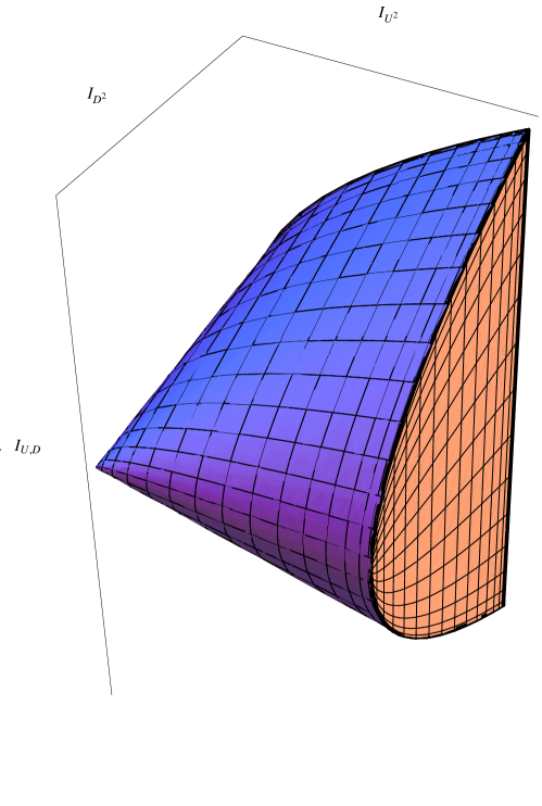
  Figure 6.1: I-manifold spanned by $\mathcal{G}_{\mathcal{F}}^{q}$ invariants built with $\mathcal{Y}_{U,D}$ for fixed $I_{U}$ , $I_{D}$ and 2 quark generations - The boundaries of this manifold correspond to configurations of flavour fields that leave and unbroken symmetry. The vertex to the left is associated to degenerate up and down sectors and a $U(2)$ symmetry. The upper and lower vertexes on the right correspond to a $U(1)^{4}$ symmetry, hierarchical up and down sectors and mixing angle vanishing or $\pi/2$ respectively. The parabola joining these two last points seen (unseen) on the figure corresponds to hierarchical up (down) sector and $0$ or $\pi/2$ mixing angle leaving an $U(1)^{3}$ unbroken symmetry. These vertexes and parabolae are the only configurations that the renormalizable potential allows for.

  Summarizing, the total Jacobian determinant is:

  $$\det J=-64\,y_{u}y_{d}y_{s}y_{c}\,\sin{2\theta_{c}}\left(y_{c}^{2}-y_{u}^{2}\right)^{2}\left(y_{s}^{2}-y_{d}^{2}\right)^{2}\,$$ (6.53)

  and the two largest subgroups of $\mathcal{G}_{\mathcal{F}}^{q}$ are $U(2)$ and $U(1)^{4}$ associated to two singular points: the vertex point of the Fig. 6.1 and the upper corner of the same figure respectively.

• Explicitly axial breaking case: $\mathcal{G}_{\mathcal{F}}^{\not{A},q}\sim SU(n_{g})^{3}$ - The invariants differ in this case and so do the Jacobians:

  $$J_{U}=\partial_{y}\left(\mbox{Tr}\left(\mathcal{Y}_{U}\mathcal{Y}_{U}^{\dagger}\right)\,,\,\det\mathcal{Y}_{U}\right)=\left(\begin{array}[]{cc}2y_{u}&y_{c}\\ 2y_{c}&y_{u}\\ \end{array}\right)\,,$$ (6.54)

  and

  $$J_{D}=\partial_{y}\left(\mbox{Tr}\left(\mathcal{Y}_{D}\mathcal{Y}_{D}^{\dagger}\right)\,,\,\det\mathcal{Y}_{D}\right)=\left(\begin{array}[]{cc}2y_{d}&y_{s}\\ 2y_{s}&y_{d}\\ \end{array}\right)\,,$$ (6.55)

  so that

  $$\det J_{U}=2(y_{u}^{2}-y_{c}^{2})\,,\qquad\qquad\det J_{D}=2(y_{d}^{2}-y_{s}^{2})\,,$$ (6.56)

  and the single solution associated to the pattern $\mathcal{G}_{\mathcal{F}}^{q}\rightarrow SU(2)_{V}\times U(1)_{B}$ survives since now no axial symmetry is present from the beginning. The single boundary in this case as opposed to the axial preserving case can be identified in the general inequalities:

  $$|I_{\tilde{U}}|\leq\frac{1}{2}I_{U}\,,\qquad\qquad|I_{\tilde{D}}|\leq\frac{1}{2}I_{D}\,,$$ (6.57)

  which are saturated for degenerate masses only $y_{c,s}=y_{u,d}$.

  The third invariant related to the phase $\phi_{U,D}$ can be taken to be $\mbox{Arg}\left(\det\mathcal{Y}_{U,D}\right)$, which is no other than the variable itself. Then this part of the Jacobian is block diagonal and constant, such that the determinant of the Jacobian stays the same.

  Altogether the Jacobian determinant is:

  $$\det J=-4\sin{2\theta_{c}}\,\left(y_{c}^{2}-y_{u}^{2}\right)^{2}\left(y_{s}^{2}-y_{d}^{2}\right)^{2}\,,$$ (6.58)

  and the only maximal subgroup is $U(2)_{V}$.

6.1.1.2 The Potential at the Renormalizable Level

The study of the Jacobian helped identify simple solutions in which some subgroup of $\mathcal{G}_{\mathcal{F}}^{q}$ was left unbroken corresponding to boundaries of the I-manifold. This analysis will serve as guide in the evaluation of the general scalar potential at the renormalizable level and the set of minima it allows for. The following study will reveal features obscured in the Jacobian method and will give further insight about the possible configurations and the role of unbroken symmetries. In particular it will reveal which of the above extrema (boundaries) correspond to minima and whether the potential allows for solutions outside of the boundaries and of what kind.

Axial preserving case: $\mathcal{G}_{\mathcal{F}}^{q}\sim U(n_{g})^{3}$

The most general renormalizable potential invariant under the whole flavour symmetry group $\mathcal{G}_{F}^{q}$ can be written in a compact manner by means of the introduction of the array:

$$X\equiv \left(I_{U},I_{D}\right)^{T}=\left(\mbox{Tr}\left(\mathcal{Y}_{U}\mathcal{Y}_{U}^{\dagger}\right),\mbox{Tr}\left(\mathcal{Y}_{D}\mathcal{Y}_{D}^{\dagger}\right)\right)^{T}\,,$$ (6.59)

in terms of which:

$$V^{(4)}= -\mu^{2}\cdot X+X^{T}\cdot\lambda\cdot X+g\,\mbox{Tr}\left(\mathcal{Y}_{U}\mathcal{Y}_{U}^{\dagger}\mathcal{Y}_{D}\mathcal{Y}_{D}^{\dagger}\right)$$

$$+h_{U}\mbox{Tr}\left(\mathcal{Y}_{U}\mathcal{Y}_{U}^{\dagger}\mathcal{Y}_{U}\mathcal{Y}_{U}^{\dagger}\right)+h_{D}\mbox{Tr}\left(\mathcal{Y}_{D}\mathcal{Y}_{D}^{\dagger}\mathcal{Y}_{D}\mathcal{Y}_{D}^{\dagger}\right)\,,$$ (6.60)

where $\lambda$ is a $2\times 2$ real symmetric matrix, $\mu^{2}$ a real 2-vector and $h_{U,D},g$ three real parameters: a total of 8 parameters enter this potential. Strict naturalness criteria would require all dimensionless couplings $\lambda$, $h_{U,D}$ and $g$ to be of order $1$, and the dimensionful $\mu$-terms to be of the same order of magnitude of $\Lambda_{f}$ but below to ensure the EFT convergence. The evaluation of the possible minima will reveal next nonetheless that even relaxing this condition the set of possible vacua is severely restricted.

Although it is not the full solution to the minimization procedure, let us consider in a first step and for illustration the first two terms in 6.60, taking the limit $g,h_{U,D}\rightarrow 0$. We can rewrite this part, if the matrix $\lambda$ is invertible as:

$$-\mu^{2}\cdot X+X^{T}\cdot\lambda\cdot X=\left(X-\frac{1}{2}\lambda^{-1}\cdot\mu^{2}\right)^{T}\lambda\left(X-\frac{1}{2}\lambda^{-1}\cdot\mu^{2}\right)-\mu^{2}\cdot\frac{\lambda^{-1}}{4}\cdot\mu^{2}$$ (6.61)

which is the generalization of a mexican-hat potential for two invariants. It is clear that if the “vector” $\frac{1}{2}\lambda^{-1}\cdot\mu^{2}$ takes positive values the minimum would set:

$$\left(\begin{array}[]{c}I_{U}\\ I_{D}\\ \end{array}\right)=\Lambda_{f}^{2}\left(\begin{array}[]{c}y_{c}^{2}+y_{u}^{2}\\ y_{s}^{2}+y_{d}^{2}\\ \end{array}\right)=\frac{1}{2}\lambda^{-1}\cdot\mu^{2}$$ (6.62)

This equation sets the order of magnitude of the Yukawa couplings as $y\sim\mu/(\Lambda_{f}\sqrt{\lambda})$, which signals the ratio of the mass scale of the scalar fields and the high scale $\Lambda_{f}$. For generic values of $\mu^{2}$ and $\lambda$ nonetheless the Yukawa magnitude of up and down quarks would be the same, so that the two entries of $\lambda^{-1}\cdot\mu^{2}$ should accommodate certain tuning, in the two family case under consideration it would imply a $\mathcal{O}(10\%)$ ratio $y_{s}/y_{c}\simeq 10^{-1}=\sqrt{(\lambda^{-1}\mu^{2})_{U}}/\sqrt{(\lambda^{-1}\mu^{2})_{D}}.$. However let us recall here that for simplicity the coupling of the up and down scalar fields in the Yukawa operators were assumed the same, but if we were to extend this case to a two Higgs doublet scenario for example, the value of $\tan\beta$ could make this tuning disappear. As shown next, it is the hierarchies within each up and down sector that the potential is unavoidably responsible for in this scheme.

For the complete minimization the extension of the above is simple, the effect of the invariants left out $I_{U,D,UD}$ adds up to a modified $\lambda$ as shown in the appendix, Sec. 10.1.

The stepwise strategy for minimization starts with the minimization in those variables that appear less often in the potential, so that after solving in their minima equations the left-over potential no longer depends on them. Then the next variable which appears less often is selected and the process iterated again in this matrioska like fashion.

The starting point is then the angle variable, appearing in one invariant only, then follows the minimization of a variable independent from Tr$(\mathcal{Y}_{U,D}^{\dagger}\mathcal{Y}_{U,D})$, which appears most often in the potential. The variables used in particular can be taken to be the differences of eigenvalues Tr$(\mathcal{Y}_{U,D}(-\sigma_{3})\mathcal{Y}_{U,D}^{\dagger})=\Lambda_{f}^{2}\left(y_{c,s}^{2}-y_{u,d}^{2}\right)$. The values of these variables will determine the hierarchy among the different generations, whereas Tr$(\mathcal{Y}_{U,D}\mathcal{Y}_{U,D}^{\dagger})$ will have an impact on the overall magnitude of the Yukawas.

This method dictates therefore that we start with the mixing angle, that appears in the single invariant $I_{UD}$. The equation for the angle is,

$$\dfrac{\partial V^{(4)}}{\partial\theta_{c}}=g\dfrac{\partial{{I_{UD}}}}{\partial\theta_{c}}=-g\,\Lambda_{f}^{4}\sin{2\theta_{c}}\left(y_{c}^{2}-y_{u}^{2}\right)\left(y_{s}^{2}-y_{d}^{2}\right)=0\,.$$ (6.63)

The minimum of the scalar potential thus occurs for $\sin\theta_{c}=0$ or $\cos\theta_{c}=0$, for non-degenerate quark masses, which is the only case in which the angle makes physical sense. For determining which of these options is selected and to provide a very useful and general understanding of the minimization in unitary matrices parameters, the Von Neumann trace inequality for positive definite hermitian matrices is here reproduced:

Let two hermitian positive definite $j\times j$ matrices A and B have eigenvalues of moduli $\alpha_{1}\leq\alpha_{2}\leq...\leq\alpha_{j}$ and $\beta_{1}\leq\beta_{2}\leq...\leq\beta_{j}$ respectively, then the following inequality holds:

$$\sum_{i=1}^{j}\alpha_{j+1-i}\,\beta_{i}\leq\mbox{Tr}\left(A\,B\right)\leq\sum_{i=1}^{j}\alpha_{i}\beta_{i}\,.$$ (6.64)

The usefulness of this inequality is that it tells us that, considering the eigenvalues at a fixed value and varying the rest of parameters in the matrix, that is, the mixing parameters in the unitary matrices, the extrema are found for trivial unitary matrices. The inequality applied in the case of the invariant $I_{UD}$:

$$y_{u}^{2}y_{s}^{2}+y_{d}^{2}y_{c}^{2}\leq\mbox{Tr}\left(V_{C}^{\dagger}\mathbf{y}_{U}^{2}\,V_{C}\,\mathbf{y}_{D}^{2}\right)\leq y_{u}^{2}y_{d}^{2}+y_{s}^{2}y_{c}^{2}\,.$$ (6.65)

The two extrema are indeed given by the two solutions for the angle in Eq. 6.63. Which of these two is selected depends nonetheless on the sign of the coefficient in front of the invariant in the potential:

• $g>0$ The potential is minimized when $I_{UD}$ is minimized, which through Eq. 6.65 corresponds to:

  $$V_{C}=\left(\begin{array}[]{cc}0&1\\ 1&0\\ \end{array}\right)\,,\qquad\theta_{c}=\pi/2\,,$$ (6.66)

  and the situation is such that the charm quark would couple only to the down type quark and the up to the strange, in an ‘inverted hierarchy” scenario.

• $g<0$ The potential is minimized when $I_{UD}$ is maximized, so Eq. 6.65 determines:

  $$V_{C}=\left(\begin{array}[]{cc}1&0\\ 0&1\\ \end{array}\right)\,,\qquad\theta_{c}=0\,,$$ (6.67)

  This case is closer to reality, now the Cabibbo angle is set to 0 and the charm only couples to the strange quark, and the up to the down.

One can check that both these configurations leave an invariant $U(1)_{V}^{2}$ as defined in Eq. 6.41.

All in all, the straightforward lesson that follows from Eq. 6.63 is that, given the mass splittings observed in nature, the scalar potential for bi-fundamental flavour fields does not allow mixing at the renormalizable level.

The next step is the minimization in eigenvalues differences. The first relevant point is that only the invariants $I_{U^{2}},I_{D^{2}},I_{U,D}$ of Eqs. 6.13-6.14 depend on the differences of eigenvalues squared; this is explicit in Eq. 6.14 for $I_{UD}$ whereas for $I_{U^{2},D^{2}}$,

$$I_{U^{2}}= \Lambda_{f}^{4}\left(y_{u}^{4}+y_{c}^{4}\right)=\frac{\Lambda_{f}^{4}}{2}\left((y_{u}^{2}+y_{c}^{2})^{2}+(y_{u}^{2}-y_{c}^{2})^{2}\right)\,,$$ (6.68)

$$I_{D^{2}}= \Lambda_{f}^{4}\left(y_{d}^{4}+y_{s}^{4}\right)=\frac{\Lambda_{f}^{4}}{2}\left((y_{d}^{2}+y_{s}^{2})^{2}+(y_{d}^{2}-y_{s}^{2})^{2}\right)\,.$$ (6.69)

All these invariants appear linearly in the potential, Eq. 6.60.

Before entering the different possible solutions for the hierarchy of eigenvalues, a intuitive view of the potential behavior is given to identify the solution which is relevant phenomenologically.

When the operators in Eq. 6.13 have negative coefficients in Eq. 6.60. ($h_{U,D}<0$) the potential diminishes towards the hierarchical configuration, which maximizes $I_{U^{2},D^{2}}$ and minimizes $-|h_{U,D}|\,I_{U^{2},D^{2}}$. In the case of $I_{UD}$ after we substitute in Eq. 6.14 and subsequently in Eq. 6.60 the two possible solutions for the mixing at the minimum for each sign of $g$, Eqs. 6.66,6.67. The term left does no longer depend on the angle but it does depend on the product of mass differences:

$$V\supset gI_{U,D}\Big{|}_{\left\langle\theta_{c}\right\rangle}=\frac{\Lambda_{f}^{4}}{2}\left[g\left(y_{c}^{2}+y_{u}^{2}\right)\left(y_{s}^{2}+y_{d}^{2}\right)-|g|\left(y_{c}^{2}-y_{u}^{2}\right)\left(y_{s}^{2}-y_{d}^{2}\right)\right]\,,$$ (6.70)

such that it always pushes towards the hierarchical configuration for both up and down type quarks. Therefore for negative $h_{U,D}$ and $g$ the minimum will correspond to a hierarchical mass configuration without mixing. For the resemblance of nature this configuration (associated to case 1 of Eq. 6.27 in the Jacobian analysis) is a good first approximation: only the heaviest family is massive so that $y_{u}=y_{d}=0$ and the mixing is vanishing.

For completeness all the possible minima and their connection to the potential parameters are listed below (again for $g<0$):

• In this configuration a strong hierarchy arises,

  $$\mathcal{Y}_{D}=\Lambda_{f}\left(\begin{array}[]{cc}0&0\\ 0&y_{s}\\ \end{array}\right)\,,\qquad\qquad\mathcal{Y}_{U}=\Lambda_{f}\left(\begin{array}[]{cc}0&0\\ 0&y_{c}\\ \end{array}\right)\,,$$ (6.71)

  which presents an unbroken symmetry $\mathcal{G}_{\mathcal{F}}^{q}\rightarrow U(1)_{V}^{2}\times U(1)_{A}^{2}$ and is just case 1 in the Jacobian analysis, see 6.27.

• This case forbids mass for the up quark

  $$\mathcal{Y}_{D}=\Lambda_{f}\left(\begin{array}[]{cc}y_{d}&0\\ 0&y_{s}\\ \end{array}\right)\,,\qquad\qquad\mathcal{Y}_{U}=\Lambda_{f}\left(\begin{array}[]{cc}0&0\\ 0&y_{c}\\ \end{array}\right)\,,$$ (6.72)

  whereas the mass difference in the down sector is set by the relation

  $$\frac{y_{s}^{2}-y_{d}^{2}}{y_{s}^{2}+y_{d}^{2}}=\frac{-g}{2h_{D}}\frac{I_{U}}{I_{D}}\,,$$ (6.73)

  and the breaking pattern is $\mathcal{G}_{\mathcal{F}}^{q}\rightarrow U(1)_{V}^{2}\times U(1)_{A}$.

• The analogous of case II for massless down quark reads:

  $$\mathcal{Y}_{D}=\Lambda_{f}\left(\begin{array}[]{cc}0&0\\ 0&y_{s}\\ \end{array}\right)\,,\qquad\qquad\mathcal{Y}_{U}=\Lambda_{f}\left(\begin{array}[]{cc}y_{u}&0\\ 0&y_{c}\\ \end{array}\right)\,,$$ (6.74)

  $$\frac{y_{c}^{2}-y_{u}^{2}}{y_{c}^{2}+y_{u}^{2}}=\frac{-g}{2h_{D}}\frac{I_{D}}{I_{U}}\,,$$ (6.75)

  and again $\mathcal{G}_{\mathcal{F}}^{q}\rightarrow U(1)_{V}^{2}\times U(1)_{A}$.

• Finally a completely degenerate scenario is possible in region IV

  $$\mathcal{Y}_{D}=\Lambda_{f}\left(\begin{array}[]{cc}y^{\prime}&0\\ 0&y^{\prime}\\ \end{array}\right)\,,\qquad\qquad\mathcal{Y}_{U}=\Lambda_{f}\left(\begin{array}[]{cc}y&0\\ 0&y\\ \end{array}\right)\,,$$ (6.76)

  having now that the potential triggers $\mathcal{G}_{\mathcal{F}}^{q}\rightarrow SU(2)_{V}\times U(1)_{B}$ This scenario is very far from reality, but listed for completeness, and the analogous of case 3 and Eq. 6.30 in the Jacobian analysis.

These regions are shown in the $h_{U}-h_{D}$ plane in fig. 6.2.

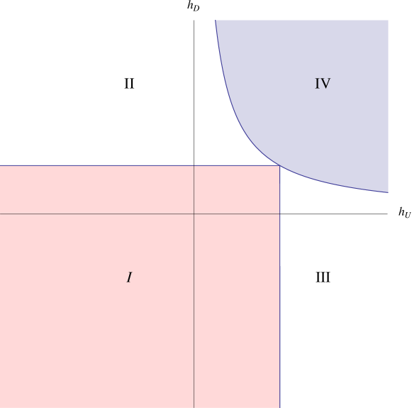
Figure 6.2: Regions for the different quark mass configurations allowed at the absolute minimum in the $h_{U}-h_{D}$ plane for $g<0$ - I is the region that yields a hierarchical spectrum for both up and down sectors. II (III) presents a hierarchical up (down) spectrum and region IV results in degenerate up and down sectors. See appendix, Sec. 10.1 for details.

Note that the cases found here are not quite the same as the ones found in the Jacobian analysis. Case 2.a (Eq. 6.28) and 2.b (Eq. 6.29) are only present in the limiting case $g\rightarrow 0$ of II (Eqs. 6.72,6.73) and III (Eqs. 6.74,6.75), so those are fine tuned cases. The reason for this is found in the symmetries, indeed cases 2.a and II and 2.b and III have the same symmetry, so from this point of view there is nothing special on having two eigenvalues degenerate in one sector when in the other sector one entry is 0. The connection of the up and down sector is due to the common group transformation properties under $SU(3)_{Q_{L}}$ of $\mathcal{Y}_{U,D}$ and indeed this correlation disappears if the mixing invariant is neglected $g\rightarrow 0$, as can be checked on Eqs. 6.73,6.75.

The singular point solutions, I and IV, are present as the absolute minima under certain conditions detailed in the appendix (10.1) but are not the only possibilities.

Explicitly axial breaking case: $\mathcal{G}_{\mathcal{F}}^{\not{A},q}\sim SU(n_{g})^{3}$

The set-up will change with the introduction of the determinants in Eq. 6.15 when choosing to violate $U(1)_{A^{U}}\times U(1)_{A^{D}}$ explicitly. By making use of the analogous of $X$ in this case,

$$\tilde{X}= \left(I_{U},I_{D},I_{\tilde{U}},I_{\tilde{D}}\right)^{T}$$ (6.77)

$$= \left(\mbox{Tr}\left(\mathcal{Y}_{U}\mathcal{Y}_{U}^{\dagger}\right),\mbox{Tr}\left(\mathcal{Y}_{D}\mathcal{Y}_{D}^{\dagger}\right),\det\left(\mathcal{Y}_{U}\right)\,,\,\det\left(\mathcal{Y}_{D}\right)\ \right)^{T}\,,$$ (6.78)

the potential reads:

$$V^{(4)}=-\tilde{\mu}^{2}\cdot\tilde{X}+\tilde{X}^{T}\cdot\tilde{\lambda}\cdot\tilde{X}+h.c.+g\,I_{UD}$$ (6.79)

where $\lambda$ is a matrix and $\mu^{2}$ a 4-vector, the entries of these two structures are complex when they involve the determinants. The number of parameters has increased now to 15 (out of which 9 are complex), since the flavour symmetry is less restrictive. Nonetheless the phases of the determinants are variables not observable at low energies and their minimization is of no interest here; suffice then to assume that they are set to their minimum values. One can then effectively consider all parameters in Eq. 6.79 real.

Parallel to the axial conserving case we have that, in the limit $g\rightarrow 0$, the minimum sets

$$\left\langle\tilde{X}\right\rangle=\frac{1}{2}\tilde{\lambda}^{-1}\cdot\tilde{\mu}^{2}\,,$$ (6.80)

if the entries of such vector are in the inside of the I-manifold. This now requires two conditions in the entries of $\tilde{\lambda}^{-1}\cdot\tilde{\mu}^{2}/2$. First, the two first entries have to be positive, since $I_{U,D}$ contained in $\tilde{X}$ are always positive; second, the condition of Eq. 6.57 must be satisfied by the associated entries of $\tilde{\lambda}^{-1}\cdot\tilde{\mu}^{2}$. If this second condition is not realized the minimum is at the boundary, that is, $I_{U}=2|I_{\tilde{U}}|$ ($I_{D}=2|I_{\tilde{D}}|$) or equivalently $y_{u}=y_{c}$ ($y_{d}=y_{s}$).

Note also that in this case the solutions I, II and III are not present just like cases 2.a and 2.b were not either in the Jacobian analysis.

These considerations together with the distinct symmetries from which they arise lead to propose an ansatz for the explanation of the hierarchy among the two generations of quarks.

First, we consider the whole $\mathcal{G}_{\mathcal{F}}^{q}$ group, so that determinants are forbidden and the minimum is in region I where the up and down are massless at this order. Then, introduction of a small source of breaking of the $U(1)_{A}$’s would allow for the appearance of determinant terms in the potential with a naturally small coefficient since it is constrained by a symmetry, and whose impact is to produce small masses for the light family.

This set-up is qualitatively explainable from symmetry considerations. In the axial preserving case the solution of hierarchical masses was present but the explicit breaking of the axial symmetry does not allow for such solutions. This means that a small perturbation on the axial symmetry breaking direction produces a small shift in the light quark masses.

6.1.1.3 The Potential at the Non-Renormalizable Level

The scalar potential at the renormalizable level in the axial preserving case allows for solutions with a strong hierarchy for both sectors of quarks, that can be perturbed via a small breaking of the axial $U(1)_{A^{U},\,A^{D}}$ to displace the minimum and lift the zero masses of the lightest quarks. The Cabibbo angle was unavoidably set to 0. In this section we explore whether non-renormalizable terms in the potential may complete the picture and produce a small Cabibbo angle.

Consider the addition of non-renormalizable operators to the scalar potential, $V^{(i>4)}$. It is interesting to notice that this does not require the introduction of new invariants beyond those in Eqs. 6.9-6.11: all higher order traces and determinants can in fact be expressed in terms of that basis of five “renormalizable” invariants.

The lowest higher dimensional contributions to the scalar potential have dimension six. At this order, the only terms involving the mixing angle are

$$V^{(6)}\supset\dfrac{1}{\Lambda_{f}^{2}}\left(\alpha_{U}I_{UD}I_{U}+\alpha_{D}I_{UD}I_{D}+\tilde{\alpha}_{U}I_{UD}I_{\tilde{U}}+\tilde{\alpha}_{D}I_{UD}I_{\tilde{D}}\right)\,.$$ (6.81)

These terms, however, show the same dependence on the Cabibbo angle previously found in Eq. (6.63) and, consequently, they can simply be absorbed in the redefinition of the lowest order parameter $g$. To find a non-trivial angular structure it turns out that terms in the potential of dimension eight (or higher) have to be considered, that is

$$V^{(8)}\supset\frac{\alpha}{\Lambda_{f}^{4}}I_{UD}^{2}\,,$$ (6.82)

with which the possibility of a mexican hat-like potential for $I_{UD}$ becomes possible

$$V^{(8)}\supset\frac{\alpha}{\Lambda_{f}^{4}}\left(I_{UD}-\frac{g}{2\alpha}\Lambda_{f}^{4}\right)^{2}\,,$$ (6.83)

which would set

$$\sin^{2}\theta\simeq\dfrac{g}{2\,y^{2}_{c}y^{2}_{s}\alpha}\,.$$ (6.84)

Using the experimental values of the Yukawa couplings $y_{s}$ and $y_{c}$, a realistic value for $\sin\theta$ can be obtained although at the price of assuming a highly fine-tuned hierarchy between the dimensionless coefficients of $d=4$ and $d=8$ terms, $g/\alpha\sim 10^{-10}$, that cannot be naturally justified in an effective Lagrangian approach.

The conclusion is therefore that mixing is absent in a natural 2 generation quark case.

6.1.2 Three Family Case

In this section we extend the approach discussed in the previous section to the three-family case. The two bi-triplets scalars $\mathcal{Y}_{U,D}$ transform explicitly under the flavour symmetry $\mathcal{G}_{F}^{q}$, as in Eq. 5.5 and the Yukawa Lagrangian is the same as that in Eq. 5.3. Once the flavons develop a vev the flavour symmetry is broken and one should recover the observed fermion masses and CKM matrix given by Eq. 5.4.

While most of the procedure follows the steps of the 2 generation case, a few differences shall be underlined. First, the number of variables and therefore independent invariants differs. As in the two family case, we can absorb three unitary matrices with $\mathcal{G_{F}}$ rotations to leave two diagonal matrices with 3 eigenvalues each and a unitary matrix. The latter contains three angles and 6 phases; diagonal complex phase transformations allow to eliminate 5 of these, so that the unitary matrix contains 4 physical parameters. In total 10 parameters describe the axial preserving case. This resembles closely the usual discussion of physical flavour parameters as expected.

The higher number of variables implies that the set of invariants extends beyond mass dimension 4 and therefore not all of them will be present at the renormalizable level.

The list of invariants now reads (102, 99):

$$I_{U} =\mbox{Tr}\left[\mathcal{Y}_{U}\mathcal{Y}_{U}^{\dagger}\right]\,, I_{D} =\mbox{Tr}\left[\mathcal{Y}_{D}\mathcal{Y}_{D}^{\dagger}\right]\,,$$ (6.85)

$$I_{U^{2}} =\mbox{Tr}\left[\left(\mathcal{Y}_{U}\mathcal{Y}_{U}^{\dagger}\right)^{2}\right]\,, I_{D^{2}} =\mbox{Tr}\left[\left(\mathcal{Y}_{D}\mathcal{Y}_{D}^{\dagger}\right)^{2}\right]\,,$$ (6.86)

$$I_{U^{3}} =\mbox{Tr}\left[\left(\mathcal{Y}_{U}\mathcal{Y}_{U}^{\dagger}\right)^{3}\right]\,, I_{D^{3}} =\mbox{Tr}\left[\left(\mathcal{Y}_{D}\mathcal{Y}_{D}^{\dagger}\right)^{3}\right]\,,$$ (6.87)

these first 6 invariants depend only on eigenvalues while the following 4 contain mixing too,

$$I_{U,D} =\mbox{Tr}\left[\mathcal{Y}_{U}\mathcal{Y}_{U}^{\dagger}\mathcal{Y}_{D}\mathcal{Y}_{D}^{\dagger}\right]\,, I_{U,D^{2}} =\mbox{Tr}\left[\mathcal{Y}_{U}\mathcal{Y}_{U}^{\dagger}\left(\mathcal{Y}_{D}\mathcal{Y}_{D}^{\dagger}\right)^{2}\right]\,,$$ (6.88)

$$I_{U^{2},D} =\mbox{Tr}\left[\mathcal{Y}_{U}\mathcal{Y}_{U}^{\dagger}\left(\mathcal{Y}_{D}\mathcal{Y}_{D}^{\dagger}\right)^{2}\right]\,, I_{(U,D)^{2}} =\mbox{Tr}\left[\left(\mathcal{Y}_{U}\mathcal{Y}_{U}^{\dagger}\mathcal{Y}_{D}\mathcal{Y}_{D}^{\dagger}\right)^{2}\right]\,.$$ (6.89)

Explicitly these invariants read:

$$I_{U} =\Lambda_{f}^{2}\sum y_{\alpha}^{2}\,, I_{D} =\Lambda_{f}^{2}\sum y_{i}^{2}\,,$$ (6.90)

$$I_{U^{2}} =\Lambda_{f}^{4}\sum y_{\alpha}^{4}\,, I_{D^{2}} =\Lambda_{f}^{4}\sum y_{i}^{4}\,,$$ (6.91)

$$I_{U^{3}} =\Lambda_{f}^{6}\sum y_{\alpha}^{6}\,, I_{D^{6}} =\Lambda_{f}^{6}\sum y_{i}^{6}\,,$$ (6.92)

$$I_{U,D} =\Lambda_{f}^{4}\sum y_{\alpha}^{2}V_{\alpha i}y_{i}^{2}V^{*}_{\alpha i}\,, I_{U,D^{2}} =\Lambda_{f}^{6}\sum y_{\alpha}^{2}V_{\alpha i}y_{i}^{4}V^{*}_{\alpha i}\,,$$ (6.93)

$$I_{U^{2},D} =\Lambda_{f}^{6}\sum y_{\alpha}^{4}V_{\alpha i}y_{i}^{2}V^{*}_{\alpha i}\,, I_{(U,D)^{2}} =\Lambda_{f}^{8}\sum\,y_{\alpha}^{2}\,V_{\alpha i}\,y_{i}^{2}\,V_{\beta i}^{*}\,y_{\beta}^{2}\,V_{\beta j}\,y_{j}^{2}\,V_{\alpha j}^{*}\,,$$ (6.94)

In the explicitly axial breaking case two complex phases add to the previous number of parameters so that 12 altogether conform the total. In this case the determinants

$$I_{\tilde{U}} =\det\left(\mathcal{Y}_{U}\right)\,, I_{\tilde{D}} =\det\left(\mathcal{Y}_{D}\right)\,,$$ (6.95)

substitute the invariants in Eq. 6.87 since they are connected through the relations:

$$\mbox{Tr}\left(\left(\mathcal{Y}_{U}^{\dagger}\mathcal{Y}_{U}\right)^{3}\right)= \frac{3}{2}\mbox{Tr}\left(\left(\mathcal{Y}_{U}^{\dagger}\mathcal{Y}_{U}\right)^{2}\right)\mbox{Tr}\left(\mathcal{Y}_{U}^{\dagger}\mathcal{Y}_{U}\right)$$

$$-\frac{1}{2}\left(\mbox{Tr}\left(\mathcal{Y}_{U}^{\dagger}\mathcal{Y}_{U}\right)\right)^{3}+3\det\mathcal{Y}_{U}\det\mathcal{Y}_{U}^{\dagger}$$ (6.96)

$$\mbox{Tr}\left(\left(\mathcal{Y}_{D}^{\dagger}\mathcal{Y}_{D}\right)^{3}\right)= \frac{3}{2}\mbox{Tr}\left(\left(\mathcal{Y}_{D}^{\dagger}\mathcal{Y}_{D}\right)^{2}\right)\mbox{Tr}\left(\mathcal{Y}_{D}^{\dagger}\mathcal{Y}_{D}\right)$$

$$-\frac{1}{2}\left(\mbox{Tr}\left(\mathcal{Y}_{D}^{\dagger}\mathcal{Y}_{D}\right)\right)^{3}+3\det\mathcal{Y}_{D}\det\mathcal{Y}_{D}^{\dagger}$$ (6.97)

and they read in terms of the variables,

$$I_{\tilde{U}} =\Lambda_{f}^{3}e^{i\phi_{U}}\prod y_{\alpha}\,, I_{\tilde{D}} =\Lambda_{f}^{3}e^{i\phi_{U}}\prod y_{i}\,,$$ (6.98)

which makes clear that the determinants of the fields change to mass dimension 3 in the present 3 family case.

6.1.2.1 The Jacobian

The study of the Jacobian is developed next. The Jacobian has an structure as in Eq. 6.20. For the mass terms the analysis was first carried out in (19, 110), while for the mixing we refer to (17).

Let’s turn first to the mixing Jacobian $J_{UD}$. We know that 4 parameters suffice to describe the mixing. Rather than choosing a parametrization for $V_{CKM}$, let us use the properties of a unitary matrix, substituting Eq. 6.5 in $I_{U,D}$:

$$\Lambda_{f}^{-4}I_{U,D} = \sum_{\alpha,i}^{3}y_{\alpha}^{2}\,V_{\alpha i}\,y_{i}^{2}\,V_{\alpha i}^{*}\,,$$ (6.99)

$$= \sum_{\alpha,i}^{3,2}y_{\alpha}^{2}V_{\alpha i}\left(y_{i}^{2}-y_{b}^{2}\right)V_{\alpha i}^{*}+y_{b}^{2}\sum_{\alpha}y_{\alpha}^{2}\,,$$ (6.100)

$$= \sum_{\alpha,i}^{2}\left(y_{\alpha}^{2}-y_{t}^{2}\right)V_{\alpha i}\left(y_{i}^{2}-y_{b}^{2}\right)V_{\alpha i}^{*}\,,+y_{b}^{2}\sum_{\alpha}y_{\alpha}^{2}+y_{t}^{2}\sum_{i}y_{i}^{2}\,,$$ (6.101)

where the terms independent of mixing elements are irrelevant for the analysis and will not be kept in the following. Note that what is achieved in using the unitarity relations is to rewrite the invariant in terms of 4 mixing elements, namely $|V_{ud}|,|V_{us}|,|V_{cd}|$ and $|V_{cs}|$. The choice of these 4 is of course to one’s discretion; we can choose other 4 by removing the $\alpha^{\prime}th$ row and the $i^{\prime}th$ column of $V_{CKM}$.

The same procedure for $I_{U,D^{2}}$ and $I_{U^{2},D}$ yields:

$$\Lambda_{f}^{-6}I_{U,D^{2}} =\sum_{\alpha,i}^{2}\left(y_{\alpha}^{2}-y_{t}^{2}\right)V_{\alpha i}\left(y_{i}^{2}+y_{b}^{2}\right)\left(y_{i}^{2}-y_{b}^{2}\right)V_{\alpha i}^{*}+\cdots\,,$$ (6.102)

$$\Lambda_{f}^{-6}I_{U^{2},D} =\sum_{\alpha,i}^{2}\left(y_{\alpha}^{2}+y_{t}^{2}\right)\left(y_{\alpha}^{2}-y_{t}^{2}\right)V_{\alpha i}\left(y_{i}^{2}-y_{b}^{2}\right)V_{\alpha i}^{*}+\cdots\,,$$ (6.103)

whereas $I_{(U,D)^{2}}$ is more involved:

$$\Lambda_{f}^{-8}I_{(U,D)^{2}}=\sum_{\alpha,\beta,i,j}^{3}\,\left(y_{\alpha}^{2}-y_{t}^{2}\right)\,V_{\alpha i}\,\left(y_{i}^{2}-y_{b}^{2}\right)\,V_{\beta i}^{*}\,\left(y_{\beta}^{2}-y_{t}^{2}\right)\,V_{\beta j}\,\left(y_{j}^{2}-y_{b}^{2}\right)\,V_{\alpha j}^{*}+\cdots\,,$$ (6.104)

this equation differs from the square of $I_{U,D}$, in terms in which $\beta\neq\alpha$ and $i\neq j$, which implies they are all proportional to 4 different mass differences:

$$\Lambda_{f}^{-8}I_{(U,D)^{2}} = \left(\sum_{\alpha,i}^{3}y_{\alpha}^{2}\,V_{\alpha i}\,y_{i}^{2}\,V_{\alpha i}^{*}\right)^{2}-2\left(y_{u}^{2}-y_{t}^{2}\right)\left(y_{c}^{2}-y_{t}^{2}\right)\left(y_{d}^{2}-y_{b}^{2}\right)\left(y_{s}^{2}-y_{b}^{2}\right)$$ (6.105)

$$\times\left(V_{ud}V_{cs}-V_{us}V_{cd}\right)\left(V^{*}_{ud}V^{*}_{cs}-V^{*}_{us}V^{*}_{cd}\right)\,.$$

The first part is not relevant as it is a function of a previously categorized invariant. The second though, has a peculiar dependence on the mixing parameters. To rewrite it in terms of the four independent parameters chosen here the following relation is used:

$$\det\left(V\right)\det\left(V^{*}\right)=\sum_{\alpha,i}^{2}V_{\alpha i}V_{\alpha i}^{*}-\left(V_{ud}V_{cs}-V_{us}V_{cd}\right)\left(V^{*}_{ud}V^{*}_{cs}-V^{*}_{us}V^{*}_{cd}\right)=1\,.$$ (6.106)

Resuming, the 4 independent pieces of the invariants:

$$I^{\prime}_{U,D} =\sum_{\alpha,i}\left(y_{\alpha}^{2}-y_{t}^{2}\right)\left(y_{i}^{2}-y_{b}^{2}\right)V_{\alpha i}V_{\alpha i}^{*}\,,$$ (6.107)

$$I^{\prime}_{U,D^{2}} =\sum_{\alpha,i}\left(y_{\alpha}^{2}-y_{t}^{2}\right)\left(y_{i}^{2}+y_{b}^{2}\right)\left(y_{i}^{2}-y_{b}^{2}\right)V_{\alpha i}V_{\alpha i}^{*}\,,$$ (6.108)

$$I^{\prime}_{U^{2},D} =\sum_{\alpha,i}\left(y_{\alpha}^{2}+y_{t}^{2}\right)\left(y_{\alpha}^{2}-y_{t}^{2}\right)\left(y_{i}^{2}-y_{b}^{2}\right)V_{\alpha i}V_{\alpha i}^{*}\,,$$ (6.109)

$$I^{\prime}_{(U,D)^{2}} =\prod_{\beta}\left(y_{\beta}^{2}-y_{t}^{2}\right)\prod_{j}\left(y_{j}^{2}-y_{b}^{2}\right)\sum_{\alpha,i}^{2}V_{\alpha i}V_{\alpha i}^{*}\,,$$ (6.110)

build up the Jacobian

$$J_{UD}=\frac{\partial I^{\prime}}{\partial|V_{\alpha,i}|}\propto\left(\begin{array}[]{cccc}|V_{ud}|&\left(y_{d}^{2}+y_{b}^{2}\right)|V_{ud}|&\left(y_{u}^{2}+y_{t}^{2}\right)|V_{ud}|&\left(y_{c}^{2}-y_{t}^{2}\right)\left(y_{s}^{2}-y_{b}^{2}\right)|V_{ud}|\\[2.84526pt] |V_{us}|&\left(y_{s}^{2}+y_{b}^{2}\right)|V_{us}|&\left(y_{u}^{2}+y_{t}^{2}\right)|V_{us}|&\left(y_{c}^{2}-y_{t}^{2}\right)\left(y_{d}^{2}-y_{b}^{2}\right)|V_{us}|\\[2.84526pt] |V_{cd}|&\left(y_{d}^{2}+y_{b}^{2}\right)|V_{cd}|&\left(y_{c}^{2}+y_{t}^{2}\right)|V_{cd}|&\left(y_{u}^{2}-y_{t}^{2}\right)\left(y_{s}^{2}-y_{b}^{2}\right)|V_{cd}|\\[2.84526pt] |V_{cs}|&\left(y_{s}^{2}+y_{b}^{2}\right)|V_{cs}|&\left(y_{c}^{2}+y_{t}^{2}\right)|V_{cs}|&\left(y_{u}^{2}-y_{t}^{2}\right)\left(y_{d}^{2}-y_{b}^{2}\right)|V_{cs}|\end{array}\right)$$ (6.111)

where the proportionality constant is different for each row, namely the product $\left(y_{\alpha}^{2}-y_{t}^{2}\right)\left(y_{i}^{2}-y_{b}^{2}\right)$. The determinant of $J_{UD}$ is

$$\det\left(J_{UD}\right)= \left(y_{u}^{2}-y_{t}^{2}\right)\left(y_{t}^{2}-y_{c}^{2}\right)\left(y_{c}^{2}-y_{u}^{2}\right)\left(y_{d}^{2}-y_{b}^{2}\right)\left(y_{b}^{2}-y_{s}^{2}\right)\left(y_{s}^{2}-y_{d}^{2}\right)$$

$$\times|V_{ud}||V_{us}||V_{cd}||V_{cs}|$$ (6.112)

The analysis has turned out to be as simple as it could be. The determinant vanishes if any of the mass differences does, or if any of the entries of $V_{CKM}$ vanishes. The rank is reduced the most for three vanishing mixing elements, which corresponds to (a permutation of) the identity.

Next, the analysis of the invariants containing eigenvalues solely is presented; the axial breaking case was analyzed in (19) but is reproduced here for completeness.

• Axial conserving case: $\mathcal{G}_{\mathcal{F}}^{q}\sim U(n_{g})^{3}$. The Jacobians are in this case,

  $$J_{U}=\partial_{\mathbf{y}_{U}}\left(\mbox{Tr}\,\mathcal{Y}_{U}\mathcal{Y}_{U}^{\dagger}\,,\,\mbox{Tr}\,(\mathcal{Y}_{U}\mathcal{Y}_{U}^{\dagger})^{2}\,,\,\mbox{Tr}\,(\mathcal{Y}_{U}\mathcal{Y}_{U}^{\dagger})^{3}\right)=\left(\begin{array}[]{ccc}2y_{u}&4y_{u}^{3}&6y_{u}^{5}\\[5.69054pt] 2y_{c}&4y_{c}^{3}&6y_{c}^{5}\\[5.69054pt] 2y_{t}&4y_{t}^{3}&6y_{t}^{5}\\[5.69054pt] \end{array}\right)\,,$$ (6.113)

  and

  $$J_{D}=\partial_{\mathbf{y}_{D}}\left(\mbox{Tr}\,\mathcal{Y}_{D}\mathcal{Y}_{D}^{\dagger}\,,\,\mbox{Tr}\,(\mathcal{Y}_{D}\mathcal{Y}_{D}^{\dagger})^{2}\,,\,\mbox{Tr}\,(\mathcal{Y}_{D}\mathcal{Y}_{D}^{\dagger})^{3}\right)=\left(\begin{array}[]{ccc}2y_{d}&4y_{d}^{3}&6y_{d}^{5}\\[5.69054pt] 2y_{s}&4y_{s}^{3}&6y_{s}^{5}\\[5.69054pt] 2y_{b}&4y_{b}^{3}&6y_{b}^{5}\\[5.69054pt] \end{array}\right),$$ (6.114)

  so that:

  $$\det J_{U}=48\,y_{c}y_{u}y_{t}(y_{u}^{2}-y_{c}^{2})(y_{c}^{2}-y_{t}^{2})(y_{u}^{2}-y_{t}^{2})\,,$$ (6.115)

  $$\det J_{D}=48\,y_{d}y_{s}y_{b}(y_{d}^{2}-y_{s}^{2})(y_{s}^{2}-y_{b}^{2})(y_{d}^{2}-y_{b}^{2})\,.$$ (6.116)

  There are now 6 possibilities to cancel each determinant above with ordered eigenvalues. These can be shorted in those who reduce the rank of the Jacobian to 2,

  $$\mathcal{Y}\sim\left(\begin{array}[]{ccc}0&0&0\\ 0&y&0\\ 0&0&y^{\prime}\\ \end{array}\right),\quad\left(\begin{array}[]{ccc}y&0&0\\ 0&y&0\\ 0&0&y^{\prime}\\ \end{array}\right),\quad\left(\begin{array}[]{ccc}y&0&0\\ 0&y^{\prime}&0\\ 0&0&y^{\prime}\\ \end{array}\right),$$ (6.117)

  and those that yield a rank 1 Jacobian

  $$\mathcal{Y}\sim\left(\begin{array}[]{ccc}0&0&0\\ 0&0&0\\ 0&0&y\\ \end{array}\right),\quad\mathcal{Y}\sim\left(\begin{array}[]{ccc}0&0&0\\ 0&y&0\\ 0&0&y\\ \end{array}\right),\quad\mathcal{Y}\sim\left(\begin{array}[]{ccc}y&0&0\\ 0&y&0\\ 0&0&y\\ \end{array}\right).$$ (6.118)

  These configurations correspond to boundaries which can also be extracted from the general inequalities:

  $$I_{U^{3}}\geq \frac{I_{U}}{2}\left(3I_{U^{2}}-I_{U}^{2}\right)$$ (6.119)

  $$\left(3I_{U^{2}}-I_{U}^{2}\right)^{3}\geq 2\left(9I_{U^{3}}-9I_{U^{2}}I_{U}+2I_{U}^{3}\right)^{2}$$ (6.120)

  and analogously for the down-type invariants. The different boundaries are depicted in Fig. LABEL:BoundariesGraphU(3).

  

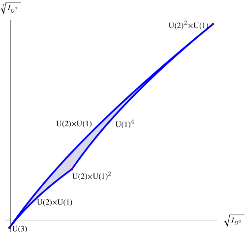
  Figure 6.3: I-manifold spanned by $\mathcal{G}_{\mathcal{F}}^{q}$ invariants built with $\mathcal{Y}_{U}$ for fixed $I_{U}$ and 3 quark generations - The study of the shape of the allowed region for the invariants $I_{U^{2}}$, $I_{U^{3}}$ reveals the different possible unbroken symmetries at the vacuum.

  We will not list all the possible combinations of the up and down sector configurations but display the three that result in the largest dimension maximal unbroken subgroups or singular points:

  1. $\mathcal{G}_{\mathcal{F}}^{q}\rightarrow SU(3)_{V}\times U(1)_{B}$   Down and Up quark sectors degenerate

     $$\mathcal{Y}_{U}=\Lambda_{f}\left(\begin{array}[]{ccc}y&0&0\\ 0&y&0\\ 0&0&y\\ \end{array}\right)\,,\qquad\quad\mathcal{Y}_{D}=\Lambda_{f}\left(\begin{array}[]{ccc}y^{\prime}&0&0\\ 0&y^{\prime}&0\\ 0&0&y^{\prime}\\ \end{array}\right)\,.$$ (6.121)

  2. $\mathcal{G}_{\mathcal{F}}^{q}\rightarrow U(2)^{3}\times U(1)_{t+b}$   Down and Up quark sectors hierarchical

     $$\mathcal{Y}_{U}=\Lambda_{f}\left(\begin{array}[]{ccc}0&0&0\\ 0&0&0\\ 0&0&y\\ \end{array}\right)\,,\qquad\quad\mathcal{Y}_{D}=\Lambda_{f}\left(\begin{array}[]{ccc}0&0&0\\ 0&0&0\\ 0&0&y^{\prime}\\ \end{array}\right)$$ (6.122)

  3. $\mathcal{G}_{\mathcal{F}}^{q}\rightarrow U(2)^{2}\times U(1)^{2}$   Two massive degenerate and one massless fermion for up-type quarks and hierarchical down sector or vice versa.

     $$\mathcal{Y}_{U}=\Lambda_{f}\left(\begin{array}[]{ccc}y&0&0\\ 0&y&0\\ 0&0&0\\ \end{array}\right)\,,\qquad\quad\mathcal{Y}_{D}=\Lambda_{f}\left(\begin{array}[]{ccc}0&0&0\\ 0&0&0\\ 0&0&y^{\prime}\\ \end{array}\right)$$ (6.123)

• Explicitly axial breaking case: $\mathcal{G}_{\mathcal{F}}^{\not{A},q}\sim SU(n_{g})^{3}$ The Jacobians read

  $$J_{U}=\partial_{y}\left(\det\mathcal{Y}_{U}\,,\,\mbox{Tr}\,\mathcal{Y}_{U}\mathcal{Y}_{U}^{\dagger}\,,\,\mbox{Tr}\,(\mathcal{Y}_{U}\mathcal{Y}_{U}^{\dagger})^{2}\right)=\left(\begin{array}[]{ccc}y_{c}y_{t}&2y_{u}&4y_{u}^{3}\\[5.69054pt] y_{t}y_{u}&2y_{c}&4y_{c}^{3}\\[5.69054pt] y_{u}y_{c}&2y_{t}&4y_{t}^{3}\\[5.69054pt] \end{array}\right)\,,$$ (6.124)

  $$J_{D}=\partial_{y}\left(\det\mathcal{Y}_{D}\,,\,\mbox{Tr}\,\mathcal{Y}_{D}\mathcal{Y}_{D}^{\dagger}\,,\,\mbox{Tr}\,(\mathcal{Y}_{D}\mathcal{Y}_{D}^{\dagger})^{2}\right)=\left(\begin{array}[]{ccc}y_{b}y_{s}&2y_{d}&4y_{d}^{3}\\[5.69054pt] y_{d}y_{b}&2y_{s}&4y_{s}^{3}\\[5.69054pt] y_{s}y_{d}&2y_{b}&4y_{b}^{3}\\[5.69054pt] \end{array}\right)\,,$$ (6.125)

  and the determinant of each Jacobian is

  $$\det J_{U}=8(y_{u}^{2}-y_{c}^{2})(y_{c}^{2}-y_{t}^{2})(y_{u}^{2}-y_{t}^{2})\,,$$ (6.126)

  $$\det J_{D}=8(y_{d}^{2}-y_{s}^{2})(y_{s}^{2}-y_{b}^{2})(y_{d}^{2}-y_{b}^{2})\,,$$ (6.127)

  from where we see that the first case in 6.117 is no longer a solution. For this case the analogous of Fig. LABEL:BoundariesGraphU(3) was first shown in (19).

6.1.2.2 The Potential at the Renormalizable Level

The following study will determine which of the different unbroken symmetries (boundaries) are respected (possible) at the different minima of the potential. The renormalizable scalar potential will contain formally the same independent invariants as in the two generation case: however these invariants now depend on a higher number of variables.

Axial preserving case: $\mathcal{G}_{\mathcal{F}}^{q}\sim U(n_{g})^{3}$

The most general scalar potential at the renormalizable level in this case is just the same formally as for the 2 family case: Eq. 6.60, using the vector X as defined in 6.59. Next, the results of the minimization process are presented.

First the Von Neumann trace inequality allows for the automatic minimization of the mixing term, so that two options arise:

$$g<0\,,\quad V_{CKM}=\left(\begin{array}[]{ccc}1&0&0\\ 0&1&0\\ 0&0&1\\ \end{array}\right)\,;\quad\quad g>0\,,\quad V_{CKM}=\left(\begin{array}[]{ccc}0&0&1\\ 0&1&0\\ 1&0&0\\ \end{array}\right).$$ (6.128)

The first is a good approximation to reality, whereas the second one would result in the top quark coupled only to the down type quark. These solutions leave an invariant generation number $U(1)^{3}_{V}$ defined as in Eq. 6.41 for generic values of masses.

The two possibilities above are a reduced number of the various permutation matrices that the Jacobian analysis singled out. This means that the potential selects some of these boundaries, concretely those that order in an inverse or direct manner the mass eigenstates of up and down sectors.

With the same procedure as for the two family case we next minimize in the variables that will determine the hierarchy. These are now the two possible eigenvalue differences in the up sector and another two in the down sector.

The potential is formally the same as in the 2 family case and let us note the “map” of Fig. 6.2 is drawn in terms of invariant magnitudes, as detailed in Sec. 10.1, such that the dimension of the matrices involved does not enter the computation. In this sense we expect the same map, as it will turn out (but only for $g<0$). It is only left to determine what are the hierarchies in these regions.

We can anticipate, focusing on the contrast with the observed flavour pattern, that a hierarchical solution corresponding to region I of Fig. 6.2 where only the heaviest family is massive and the mixing matrix is the identity is a natural possible solution. The intuitive way to guess the presence of this solution follows the argument of the two family case in the region of negative $h_{U,D}$ and $g$. The resemblance with nature in this case is good in a first sketch; top and bottom are much heavier than the rest of quarks and the mix little ($\sim\lambda_{c}^{2}$) with them.

For completeness the set of vacua is listed next for the realistic case of mixing ($g<0$):

• In this region the equivalent of the hierarchical configuration is now the case of vanishing of the lightest 4 eigenvalues,

  $$\mathcal{Y}_{D}=\Lambda_{f}\left(\begin{array}[]{ccc}0&0&0\\ 0&0&0\\ 0&0&y_{b}\\ \end{array}\right)\,,\qquad\quad\mathcal{Y}_{U}=\Lambda_{f}\left(\begin{array}[]{ccc}0&0&0\\ 0&0&0\\ 0&0&y_{t}\\ \end{array}\right)\,,$$ (6.129)

  and an unbroken $U(2)^{3}\times U(1)_{t+b}$.

• In this case we have a hierarchical Yukawa for the up sector while the two lightest down-type eigenvalues are equal:

  $$\mathcal{Y}_{D}=\Lambda_{f}\left(\begin{array}[]{ccc}y&0&0\\ 0&y&0\\ 0&0&y_{b}\\ \end{array}\right)\,,\qquad\quad\mathcal{Y}_{U}=\Lambda_{f}\left(\begin{array}[]{ccc}0&0&0\\ 0&0&0\\ 0&0&y_{t}\\ \end{array}\right)\,,$$ (6.130)

  $$y_{s}=y_{d}=y\,,\qquad\qquad\frac{y_{b}^{2}-y^{2}}{y_{b}^{2}+2y^{2}}=\frac{-g}{2h_{D}}\frac{I_{U}}{I_{D}}\,,$$ (6.131)

  leaving an unbroken an $U(2)_{V}\times U(2)_{U_{R}}\times U(1)_{t+b}$.

• III The analogous of the previous case for the up sector is

  $$\mathcal{Y}_{D}=\Lambda_{f}\left(\begin{array}[]{ccc}0&0&0\\ 0&0&0\\ 0&0&y_{b}\\ \end{array}\right)\,,\qquad\quad\mathcal{Y}_{U}=\Lambda_{f}\left(\begin{array}[]{ccc}y^{\prime}&0&0\\ 0&y^{\prime}&0\\ 0&0&y_{t}\\ \end{array}\right)\,,$$ (6.132)

  $$y_{c}=y_{u}=y\,,\qquad\qquad\frac{y_{t}^{2}-y^{\prime 2}}{y_{t}^{2}+2y^{\prime 2}}=\frac{-g}{2h_{U}}\frac{I_{D}}{I_{U}}\,,$$ (6.133)

  with an unbroken $U(2)_{V}\times U(2)_{D_{R}}\times U(1)_{t+b}$.

• IV Finally the degenerate case is simply

  $$\mathcal{Y}_{D}=\Lambda_{f}\left(\begin{array}[]{ccc}y&0&0\\ 0&y&0\\ 0&0&y\\ \end{array}\right)\,,\qquad\quad\mathcal{Y}_{U}=\Lambda_{f}\left(\begin{array}[]{ccc}y^{\prime}&0&0\\ 0&y^{\prime}&0\\ 0&0&y^{\prime}\\ \end{array}\right)\,,$$ (6.134)

  respecting a $U(3)_{V}$ symmetry.

Note that none of the solutions have a single vanishing eigenvalue, so that only the case I could be a good approximation to reality. It is the case that the potential being the same as for two families, the picture of possible vacua in Fig. 6.2 is the same, only the unbroken symmetry is different, but the maximal that we could choose (96, 97).

This is not the situation for $g>0$, in such case we expect new solutions like $\mathcal{Y}_{U}\sim$Diag$(0,y,y^{\prime})\,,\,\mathcal{Y}_{D}\sim$Diag$(y^{\prime\prime},0,0)$, which even if having an inverted hierarchy could be worth exploring.

Explicitly axial breaking case: $\mathcal{G}_{\mathcal{F}}^{\not{A},q}\sim SU(n_{g})^{3}$

The potential is now:

$$V^{(4)}= -\mu^{2}\cdot X+X^{T}\cdot\lambda\cdot X+g\,\mbox{Tr}\left(\mathcal{Y}_{U}\mathcal{Y}_{U}^{\dagger}\mathcal{Y}_{D}\mathcal{Y}_{D}^{\dagger}\right)+h_{U}\mbox{Tr}\left(\mathcal{Y}_{U}\mathcal{Y}_{U}^{\dagger}\mathcal{Y}_{U}\mathcal{Y}_{U}^{\dagger}\right)$$

$$+h_{D}\mbox{Tr}\left(\mathcal{Y}_{D}\mathcal{Y}_{D}^{\dagger}\mathcal{Y}_{D}\mathcal{Y}_{D}^{\dagger}\right)+\left(\tilde{\mu}_{U}\det\mathcal{Y}_{U}+\tilde{\mu}_{D}\det\mathcal{Y}_{D}+h.c.\right)\,.$$ (6.135)

The determinants appear only linearly in this case such that the minimization in the complex phase simplifies, for example in the case of the up-type flavour field:

$$\tilde{\mu}_{U}\det\mathcal{Y}_{U}+h.c.=|\tilde{\mu}_{U}||\det\mathcal{Y}_{U}|2\cos(\phi_{U}+\phi_{\tilde{\mu}})\rightarrow\cos(\left\langle\phi+\phi_{\tilde{\mu}}\right\rangle)=-1$$ (6.136)

so that we can consider effectively a positive determinant, $\det\mathcal{Y}_{U}>0$, and a negative coefficient, $\tilde{\mu}_{U}<0$, see (15).

The inclusion of determinants will not change the possibilities listed as I , II , III , IV, since all of these configurations are also boundaries in this case. In other words, part of the symmetries in the solutions above are still left after removing the $U(1)_{A^{U},A^{D}}$ factors, namely $SU(2)_{D_{R},E_{R}}$. This did not happen in the two family case as the unbroken symmetry was $``U(1)"$ rather than $``U(2)"$. Note however that a solution like $\mathcal{Y}\sim$Diag$(0,y^{\prime},y)$ can be perturbed by $U(1)_{A^{U},A^{D}}$ breaking terms to produce a small third eigenvalue.

6.1.2.3 The Potential at the Non-Renormalizable Level

The first issue to deal with in this case is the fact that the order of magnitude of the Yukawa eigenvalues is set by the ratio $y\sim\mu/(\Lambda_{f}\sqrt{\lambda})$ which implies for the top Yukawa that the vev of the field $\mu/\sqrt{\lambda}$ is around the scale $\Lambda_{f}$ signaling a bad convergence of the EFT. To cope with this first it is noted that the top Yukawa runs down with energy whereas the relation $y\sim\mu/(\Lambda_{f}\sqrt{\lambda})$ does not determine the overall scale $\Lambda_{f}$. For energies of the order of $10^{8}$ GeV (9) the top Yukawa is already smaller than the weak coupling constant allowing the usual expansion in EFT.

The case in which the two scales are of the same order can nonetheless formally be treated in the same sense as the non-linear $\sigma$-model, see also (111) in this regard. First the isolation in a single invariant of the problematic terms is accomplished by the set of invariants; $\{\,I_{U},I_{U^{2}}-\left(I_{U}\right)^{2},I_{U^{3}}-\left(I_{U}\right)^{3}\,\}$ instead of Eqs. 6.85-6.87, such that the latter two are suppressed by one power of the second highest eigenvalue: $y_{c}^{2}$. Terms in $I_{U}$ can be summed in a generic function in the potential $F\left(I_{U}/\Lambda_{f}^{2}\right)\equiv F(y_{t}^{\prime 2})$ where $y_{t}^{\prime}$ stands for the highest eigenvalue of $\mathcal{Y}_{U}$, different from the top Yukawa since the connection with Yukawas has also to be revisited

$$Y_{U}=\frac{\mathcal{Y}_{U}}{\Lambda_{f}}+\sum_{i}c_{i}\frac{\mathcal{Y}_{U}\left(\mathcal{Y}_{U}^{\dagger}\mathcal{Y}_{U}\right)^{i}}{\Lambda_{f}^{2i+1}}\simeq V_{CKM}^{\dagger}\left(\begin{array}[]{ccc}y_{u}&0&0\\ 0&y_{c}&0\\ 0&0&f(y_{t}^{\prime})\\ \end{array}\right).$$ (6.137)

The relation of $y_{t}^{\prime}$ with the top Yukawa coupling is then $y_{t}=f(y_{t}^{\prime})$. Then substitution in the function $F$ yields the potential as a function of the top Yukawa coupling $F(f^{-1}(y_{t}))$. This means certainly a loss in predictivity since the introduced functions $F\,,\,f$ are general, however for the present discussion it suffices that $F(f^{-1}(x))$ has a minimum at $x\simeq 1$.

In either case and to conclude this discussion, the symmetry arguments used to identify the possible vacua hold the same in this “strong interacting” scenario.

One interesting point is the possibility of non-renormalizable operators correcting the pattern of the renormalizable potential. It is a priori either a fine-tuned option like in the two family case or unsuccessful since the configurations are protected by a large unbroken symmetry. The intuitive reason for this is that for perturbations to displace the minimum they must create a small tilt in the potential via linear dependence on the deviations from the 0-order solution; however non-renormalizable terms contain high powers of eigenvalues and therefore the corrections they introduce are not linear in the perturbations.

6.2 Flavour Scalar Fields in the Fundamental

In the simplest case from the group theory point of view, each Yukawa corresponds to two scalar fields $\chi$ transforming in the fundamental representation and the Yukawa Operator has dimension 6. This approach would a priori allow to introduce one new field for each $SU(n_{g})$ component of the flavour symmetry: three fields. However, such a minimal setup leads to an unsatisfactory realization of the flavour sector as no physical mixing angle is allowed. The situation changes qualitatively, though, if two $SU(n_{g})_{Q_{L}}$ fundamental representations are introduced, one for the up and one for the down quark sectors, the field content is detailed in table 5.3.

Before discussing the potential, inspection of Eq. 5.8 will illuminate the road ahead. The hypothesis now is that Yukawas are built out of two fundamental representations. In linear algebra terms, the Yukawa matrix is made out of two vectors. This is of course a very strong assumption on the structure of the matrix. First and foremost such a matrix has rank 1, so that by construction, there is one single eigenvalue per up and down sector different from 0. Note that this statement is independent of the number of generations and the scalar potential. The situation is then a good starting approximation for a hierarchical spectrum.

Second, the number of variables in the flavour fields will now not be the same as low energy flavour observables. The scalar fields are fundamental and can be thought of as complex vectors that are “rotated” under a flavour symmetry transformation. The only physical invariants that can be associated to such vectors are the moduli and, if they live in the same space, their relative angles. Altogether the list of independent invariants and therefore physical variables describing the fields is,

$$Z=\left\{\chi_{U}^{L\dagger}\chi_{U}^{L}\,,\qquad\chi_{U}^{R\dagger}\chi_{U}^{R}\,,\qquad\chi_{D}^{L\dagger}\chi_{D}^{L}\,,\qquad\chi_{D}^{R\dagger}\chi_{D}^{R}\,,\qquad\chi_{U}^{L\dagger}\chi_{D}^{L}\,\right\}$$ (6.138)

where the array $Z$ will be useful for notation purposes; its index runs over the five values: $(U,L)\,,\,(U,R)\,,\,(D,L)\,,\,(D,R)\,,\,(U,D)$.

There is now also a clear geometrical interpretation of the mixing angle: the mixing angle between two generations of quarks is the misalignment of the $\chi^{L}$ flavons in $SU(n_{g})_{Q_{L}}$ space.

The I-manifold in this case possesses a number of boundaries identifiable studying $Z$. Indeed $Z$ does not cover all 5 dimensional space, but its components satisfy in general,

$$Z_{(U,L),(D,L),(U,R),(D,R)}\geq 0\,,$$ (6.139)

$$|Z_{(U,D)}|^{2}\leq Z_{(U,L)}Z_{(D,L)}\,,$$ (6.140)

the boundaries are reached when the above inequalities are saturated.

A word on the phenomenology of this scenario is due as well. Let us compare the phenomenology expected from bi-fundamental flavons (i.e. $d=5$ Yukawa operator) with that from fundamental flavons (i.e. $d=6$ Yukawa operators). For bi-fundamentals, the list of effective FCNC operators is exactly the same that in the original MFV proposal (26). The case of fundamentals presents some differences: higher-dimension invariants can be constructed in this case, exhibiting lower dimension than in the bi-fundamental case. For instance, one can compare these two operators:

$$\overline{D}_{R}\,\mathnormal{\mathcal{Y}_{D}}^{\dagger}\,\mathcal{Y}_{U}\,\mathcal{Y}_{U}^{\dagger}\,Q_{L}\sim[\text{mass}]^{6}\qquad\longleftrightarrow\qquad\overline{D}_{R}\,\chi_{D}^{R}\,\chi_{U}^{L\dagger}\,Q_{L}\sim[\text{mass}]^{5}\,,$$ (6.141)

where the mass dimension of the invariant is shown in brackets; with these two types of basic bilinear FCNC structures it is possible to build effective operators describing FCNC processes, but differing on the degree of suppression that they exhibit. This underlines the fact that the identification of Yukawa couplings with aggregates of two or more flavons is a setup which goes technically beyond the realization of MFV, resulting possibly in a distinct phenomenology which could provide a way to distinguish between fundamental and bi-fundamental origin.

Let us turn now to the construction of the potential.

6.2.1 The Potential at the Renormalizable Level

Previous considerations regarding the scale separation between EW and flavour breaking scale hold also in this case, and in consequence the Higgs sector contributions will not be explicitly described. The Potential for the $\chi$ fields can be written in the compact manner,

$$V^{(4)}=-\mu^{2}_{f}\cdot Z+Z^{T}\cdot\lambda_{f}\cdot Z+h.c.\,,$$ (6.142)

The total number of operators that can be introduced at the renormalizable level is 20, out of which 6 are complex. However, only 5 different combinations of these will enter the minimization equations. The solution

$$\left\langle Z\right\rangle=\frac{1}{2}\lambda^{-1}_{f}\mu_{f}^{2}\,,$$ (6.143)

exists if the vector $\lambda^{-1}_{f}\mu_{f}^{2}/2$ takes values inside the possible range of $Z$, that is the I-manifold. The case in which this does not happen leads to a boundary of the invariant space. This occurs both when at least one of the first 4 entries turns negative in $\lambda^{-1}_{f}\mu_{f}^{2}$ and the boundary is of the type of Eq. 6.139 and when $(\lambda^{-1}_{f}\mu_{f}^{2})_{(U,L)}(\lambda^{-1}_{f}\mu_{f}^{2})_{(D,L)}\leq|(\lambda^{-1}_{f}\mu_{f}^{2})_{(U,D)}|^{2}$ which corresponds to the boundary that saturates 6.140. This last case corresponds to the two vectors $\chi_{U,D}^{L}$ aligned, that precludes any mixing. This means that the no-mixing case is a boundary to which nonetheless the minima of the potential is not restricted in general.

All these considerations make straightforward the extraction of the Yukawa structure.

• Two family case - From the expressions for the Yukawa matrices in Eqs. 5.8, and the previous discussion we write that the configuration for the Yukawas is:

  $$Y_{D}=\frac{\left|\chi_{D}^{L}\right|\left|\chi_{D}^{R}\right|}{\Lambda_{f}^{2}}\left(\begin{array}[]{cc}0&0\\ 0&1\\ \end{array}\right)\,,\qquad\quad Y_{U}=\frac{\left|\chi_{U}^{L}\right|\left|\chi_{U}^{R}\right|}{\Lambda_{f}^{2}}V_{C}\left(\begin{array}[]{cc}0&0\\ 0&1\\ \end{array}\right)\,,$$ (6.144)

  $$V_{C}=\left(\begin{array}[]{cc}\cos{\theta_{c}}&\sin{\theta_{c}}\\ -\sin{\theta_{c}}&\cos{\theta_{c}}\\ \end{array}\right)\,,$$ (6.145)

  so that quark masses are fixed via Eq. 6.143 to:

  $$y_{c}=\sqrt{\frac{\left(\lambda^{-1}_{f}\mu_{f}^{2}\right)_{(U,R)}}{2\Lambda_{f}^{2}}\frac{\left(\lambda^{-1}_{f}\mu_{f}^{2}\right)_{(U,L)}}{2\Lambda_{f}^{2}}}\,,\qquad\quad y_{s}=\sqrt{\frac{\left(\lambda^{-1}_{f}\mu_{f}^{2}\right)_{(D,R)}}{2\Lambda_{f}^{2}}\frac{\left(\lambda^{-1}_{f}\mu_{f}^{2}\right)_{(D,L)}}{2\Lambda_{f}^{2}}}\,,$$ (6.146)

  $$\cos{\theta_{c}}=\frac{\left(\lambda^{-1}_{f}\mu_{f}^{2}\right)_{(U,L)}}{\sqrt{\left(\lambda^{-1}_{f}\mu_{f}^{2}\right)_{(U,L)}\left(\lambda^{-1}_{f}\mu_{f}^{2}\right)_{(D,L)}}}\,.$$ (6.147)

  The vev of the moduli of the $\chi$ fields is of the same order $\mu$ for natural parameters, so that the cosine of the Cabibbo angle above is typically of $\mathcal{O}(1)$. This means that in the fundamental case a natural scenario can give rise to both the strong hierarchies in quark masses and a non-vanishing mixing angle, whereas in the bi-fundamental case the mixing was unavoidably set to 0.

• Three family case - The extension is simple, the Yukawa matrices are still of rank one and a single mixing angle arises,

  $$Y_{D}=\frac{\left|\chi_{D}^{L}\right|\left|\chi_{D}^{R}\right|}{\Lambda_{f}^{2}}\left(\begin{array}[]{ccc}0&0&0\\ 0&0&0\\ 0&0&1\\ \end{array}\right)\,,\qquad\quad Y_{U}=\frac{\left|\chi_{U}^{L}\right|\left|\chi_{U}^{R}\right|}{\Lambda_{f}^{2}}V^{\dagger}_{CKM}\left(\begin{array}[]{ccc}0&0&0\\ 0&0&0\\ 0&0&1\\ \end{array}\right)\,.$$ (6.148)

  $$V_{CKM}=\left(\begin{array}[]{ccc}1&0&0\\ 0&\cos{\theta_{23}}&\sin{\theta_{23}}\\ 0&-\sin{\theta_{23}}&\cos{\theta_{23}}\\ \end{array}\right)\,.$$ (6.149)

  with

  $$y_{t}=\sqrt{\frac{\left(\lambda^{-1}_{f}\mu_{f}^{2}\right)_{(U,R)}}{2\Lambda_{f}^{2}}\frac{\left(\lambda^{-1}_{f}\mu_{f}^{2}\right)_{(U,L)}}{2\Lambda_{f}^{2}}}\,,\qquad\quad y_{b}=\sqrt{\frac{\left(\lambda^{-1}_{f}\mu_{f}^{2}\right)_{(D,R)}}{2\Lambda_{f}^{2}}\frac{\left(\lambda^{-1}_{f}\mu_{f}^{2}\right)_{(D,L)}}{2\Lambda_{f}^{2}}}\,,$$ (6.150)

  $$\cos{\theta_{23}}=\frac{\left(\lambda^{-1}_{f}\mu_{f}^{2}\right)_{(U,L)}}{\sqrt{\left(\lambda^{-1}_{f}\mu_{f}^{2}\right)_{U,L}\left(\lambda^{-1}_{f}\mu_{f}^{2}\right)_{(D,L)}}}\,.$$ (6.151)

  The flavour field vevs have not broken completely the flavour symmetry, leaving a residual $U(1)_{Q_{L}}\times U(2)_{D_{R}}\times U(2)_{U_{R}}\times U(1)_{B}$ symmetry group. This can be seen as follows, in the three dimensional space where $SU(3)_{Q_{L}}$ acts, the two vectors $\chi_{U,D}^{L}$ define a plane; perpendicular to this plane there is the direction of the family that is completely decoupled form the rest, and in the plane we have the massive eigenstate and the eigenstate that, even if massless, can be told from the other massless state as it mixes with the massive.

If the hierarchies in mass in each up and down sectors are explained here through the very construction of the Yukawas via fundamental fields, there is still the hierarchy of masses between the top and bottom for the potential to accommodate, that is:

$$y_{b}^{2}/y_{t}^{2}=\frac{\left(\lambda^{-1}_{f}\mu_{f}^{2}\right)_{D,R}\left(\lambda^{-1}_{f}\mu_{f}^{2}\right)_{D,L}}{\left(\lambda^{-1}_{f}\mu_{f}^{2}\right)_{U,R}\left(\lambda^{-1}_{f}\mu_{f}^{2}\right)_{U,L}}\simeq 5.7\times 10^{-4}$$ (6.152)

Note that the top-bottom hierarchy is explained in this context by the 4th power ratio of $\mu$-mass scales so that a typical ratio of $(\mu_{f})_{D}/(\mu_{f})_{U}\simeq 0.15$ suffices to explain the hierarchy.

One of the consequences of the strong hierarchy in masses imposed in this scenario is that it cannot be corrected with nonrenormalizable terms in the potential to obtain small masses for the lightest families. The reason is that the vanishing of all but one eigenvalue in the Yukawa matrices is obtained as a consequence of the scalar field fundamental content.

Nevertheless, the partial breaking of flavour symmetry provided by Eq. (6.148) can open quite interesting possibilities from a model-building point of view. Consider as an example the following multi-step approach. In a first step, only the minimal number of fundamental fields are introduced: i.e. $\chi^{L}$, $\chi^{R}_{U}$ and $\chi^{R}_{D}$. Their vevs break $SU(3)^{3}$ down to $SU(2)^{3}$, originating non-vanishing Yukawa couplings only for the top and the bottom quarks, without any mixing angle (as we have only one left-handed flavour field). As a second step, four new triplet fields $\chi^{\prime L,R}_{u,d}$ are added, whose contributions to the Yukawa terms are suppressed relatively to the previous flavons. If their vevs point in the direction of the unbroken flavour subgroup $SU(2)^{3}$, then the residual symmetry is further reduced. As a result, non-vanishing charm and strange Yukawa couplings are generated together with a mixing among the first two generations:

$$Y_{U}\equiv\frac{{\chi^{L}}\,{\chi_{U}^{R\dagger}}}{\Lambda_{f}^{2}}+\frac{{\chi_{U}^{\prime L}}\,{\chi_{U}^{\prime R\dagger}}}{\Lambda_{f}^{2}}=\left(\begin{array}[]{ccc}0&\sin{\theta_{c}}\,y_{c}&0\\ 0&\cos{\theta_{c}}\,y_{c}&0\\ 0&0&y_{t}\\ \end{array}\right)\,,$$ (6.153)

$$Y_{D}\equiv\frac{{\chi^{L}}\,{\chi_{D}^{R\dagger}}}{\Lambda_{f}^{2}}+\frac{{\chi_{D}^{\prime L}}\,{\chi_{D}^{\prime R\dagger}}}{\Lambda_{f}^{2}}=\left(\begin{array}[]{ccc}0&0&0\\ 0&y_{s}&0\\ 0&0&y_{b}\\ \end{array}\right)\,.$$

The relative suppression of the two sets of flavon vevs correspond to the hierarchy between $y_{c}$ and $y_{t}$ ($y_{s}$ and $y_{b}$). Hopefully, a refinement of this argument would allow to explain the rest of the Yukawas and the remaining angles. The construction of the scalar potential for such a setup would be quite model dependent though, and beyond the scope of this discussion.

6.3 Combining fundamentals and bi-fundamentals

Until now we have considered separately Yukawa operators of dimension $d=5$ and $d=6$. It is, however, interesting to explore if some added value from the simultaneous presence of both kinds of operators can be obtained. This is a sensible choice from the point of view of effective Lagrangians in which, working at $\mathcal{O}(1/\Lambda_{f}^{2})$, contributions of three types may be included: i) the leading $d=5$ $\mathcal{O}(1/\Lambda_{f})$ operators; ii) renormalizable terms stemming from fundamentals (i.e. from $d=6$ $\mathcal{O}(1/\Lambda_{f}^{2})$ operators; iii) other corrections numerically competitive at the orders considered here. We focus here as illustration on the impact of i) and ii):

$$\mathscr{L}_{Yukawa}=\overline{Q}_{L}\left[\dfrac{\mathnormal{\mathcal{Y}_{D}}}{\Lambda_{f}}+\dfrac{\chi_{D}^{L}\chi_{D}^{R\dagger}}{\Lambda_{f}^{2}}\right]D_{R}H+\overline{Q}_{L}\left[\dfrac{\mathcal{Y}_{U}}{\Lambda_{f}}+\dfrac{\chi_{U}^{L}\chi_{U}^{R\dagger}}{\Lambda_{f}^{2}}\right]U_{R}\tilde{H}+h.c.\,,$$ (6.154)

As the bi-fundamental flavour fields arise at first order in the $1/\Lambda_{f}$ expansion, it is suggestive to think of the fundamental contributions as a “higher order” correction. Let us then consider the case in which the flavons develop vevs as follows:

$$\dfrac{{\mathcal{Y}_{U,D}}}{\Lambda_{f}}\sim\left(\begin{array}[]{ccc}0&0&0\\ 0&0&0\\ 0&0&y_{t,b}\\ \end{array}\right)\,,\qquad\qquad\dfrac{|{\chi_{U,D}^{L}}|}{\Lambda_{f}}\sim y_{c,s}\,,$$ (6.155)

and $\chi_{U,D}^{R}$ acquire arbitrary vev values of order $\Lambda_{f}$. Finally, if the left-handed fundamental flavour fields are aligned perpendicular to the bi-fundamental fields and misaligned by $\theta_{c}$ among themselves the Yukawas read,

$$Y_{U}=\left(\begin{array}[]{ccc}0&\sin{\theta_{c}}\,y_{c}&0\\ 0&\cos{\theta_{c}}\,y_{c}&0\\ 0&0&y_{t}\\ \end{array}\right)\,,\qquad Y_{D}=\left(\begin{array}[]{ccc}0&0&0\\ 0&y_{s}&0\\ 0&0&y_{b}\\ \end{array}\right)\,.$$ (6.156)

This seems an appealing pattern, with masses for the two heavier generations and one sizable mixing angle, that we chose to identify here with the Cabibbo angle. As for the lighter family, non-vanishing masses for the up and down quarks could now result from non-renormalizable operators.

The drawback of this combined analysis is that the direct connection between the minima of the potential and the spectrum is lost and the analysis of the potential would be very involved.

7 Lepton Sector

Research in the lepton sector is at the moment in a dynamical and exciting epoch. With the recent measure of a sizable $\theta_{13}$ mixing angle (112, 113), all angles of the mixing matrix are determined and the race for discovery of CP violation in the lepton sector has started (114). At the same time there is an ambitious experimental search for flavour violation in the charged lepton sector (115, 116, 117, 118) which could pour light in possible new physics beyond the SM, and provide a new probe of the magnitude of the seesaw scale (14). On the cosmology side recent data seem to favor 3 only light species of neutrinos (119). Finally neutrinoless double beta decay searches (120) will explore one very fundamental question: are there fermions in nature which are their own antiparticle?

For the present theoretical analysis the nature of neutrino masses is crucial. If neutrinos happen to be Dirac particles, the analysis of the flavour symmetry breaking mechanism is completely analogous to that for the quark case: all conclusions drawn are directly translated to the lepton case and negligible mixing would be favored for the simplest set-up in which each Yukawa coupling is associated to a field in the bi-fundamental of the flavour group. Like for the quark case, sizable mixing would be allowed, for setups in which the Yukawas are identified with (combinations of) fields in the fundamental representation of the flavour group, implying a strong hierarchy for neutrinos.

We turn here instead to the case in which neutrinos are Majorana particles and more concretely generated by a type I seesaw model. It has been previously found (82, 83, 84, 85, 86) that for type I seesaw scenarios which exhibit approximate lepton number conservation, interesting seesaw models arise in which the effective scale of lepton number is distinct from the flavour scale yielding a testable phenomenology (86, 121, 122, 123, 124). It was first in this setup that we identified the patterns (16) to be established with more generality in the next sections. Let us consider in this chapter the general seesaw I scenario with degenerate heavy right-handed neutrinos as outlined in the introduction.

Within the hypothesis of dynamical Yukawa couplings we introduce two scalar fields in parallel to the two Yukawa matrices that are bi-fundamentals of $\mathcal{G}_{\mathcal{F}}^{l}$ as detailed in table 5.2.

7.1 Two Family Case

The counting of physical parameters goes as follows. It is known (87) that for two families with heavy degenerate neutrinos, the number of physical parameters describing the lepton sector is eight: six moduli and two phases.

Indeed, after using the freedom to choose the lepton charged matrix diagonal, as in Eq. 4.7, $Y_{\nu}$ is still a priori a general complex matrix with 8 parameters. Two phases can be absorbed through left-handed field $U(1)$ rotations and an $O(2)$ rotation on the right of the neutrino Yukawa coupling (see Eq. 5.6) reduces to five the number of physical parameters in $Y_{\nu}$, so that altogether $n=7$ parameters suffice to describe the physical degrees of freedom in the lepton Yukawas. The eight physical parameter is the heavy neutrino mass $M$. Below, for the explicit computation, we will use either the Casas-Ibarra parametrization (125) or the bi-unitary parametrization alike the quark case. The Casas-Ibarra parametrization is useful to maintain explicit the connection with masses and mixing, here it is reproduced for two families,

$$Y_{E}=\left(\begin{array}[]{cc}y_{e}&0\\ 0&y_{\mu}\\ \end{array}\right)\,,\quad\!Y_{\nu}=\frac{\sqrt{2M}}{v}\,U\,\left(\begin{array}[]{cc}\sqrt{m_{\nu_{1}}}&0\\ 0&\sqrt{m_{\nu_{2}}}\\ \end{array}\right)\,R\,,$$ (7.1)

$$U=\left(\begin{array}[]{cc}\cos{\theta}&\sin{\theta}\\ -\sin{\theta}&\cos{\theta}\\ \end{array}\right)\left(\begin{array}[]{cc}e^{i\alpha}&0\\ 0&e^{-i\alpha}\\ \end{array}\right)\,,\qquad R=\left(\begin{array}[]{cc}\cosh{\omega}&-i\sinh{\omega}\\ i\sinh{\omega}&\cosh{\omega}\\ \end{array}\right)\,.$$ (7.2)

In order to extend the parametrization above to the fields $\mathcal{Y}_{E}$, $\mathcal{Y}_{\nu}$, it is convenient to use the definitions

$$\hat{y}_{\nu_{i}}^{2}\equiv\frac{2M}{v^{2}}m_{\nu_{i}}\,,$$ (7.3)

leading to

$$\mathcal{Y}_{\nu}=\Lambda_{f}\left(\begin{array}[]{cc}\cos{\theta}&\sin{\theta}\\ -\sin{\theta}&\cos{\theta}\\ \end{array}\right)\left(\begin{array}[]{cc}e^{i\alpha}\hat{y}_{\nu_{1}}&0\\ 0&e^{-i\alpha}\hat{y}_{\nu_{2}}\\ \end{array}\right)\left(\begin{array}[]{cc}\cosh{\omega}&-i\sinh{\omega}\\ i\sinh{\omega}&\cosh{\omega}\\ \end{array}\right)\,,$$ (7.4)

$$\mathcal{Y}_{E}=\Lambda_{f}\mathbf{y}_{E}=\Lambda_{f}\left(\begin{array}[]{cc}y_{e}&0\\ 0&y_{\mu}\\ \end{array}\right)\,.$$ (7.5)

It is the case nonetheless that the minimization procedure is optimized when selecting the second type of parametrization: the bi-unitary in analogy with quarks (Eq. 4.2):

$$\mathcal{Y}_{\nu}=\Lambda_{f}\,\mathcal{U}_{L}\mathbf{y}_{\nu}\,\mathcal{U}_{R}\,,\qquad\mathcal{Y}_{E}=\Lambda_{f}\mathbf{y}_{E}\,;\qquad\qquad\mathcal{U}_{L}\,\mathcal{U}_{L}^{\dagger}=1\,,\,\,\,\,\mathcal{U}_{R}\,\mathcal{U}_{R}^{\dagger}=1\,,$$ (7.6)

with $\mathbf{y}_{E}$ as defined above, $\mathcal{U}_{L,R}$ being unitary matrices and $\mathbf{y}_{\nu}$ containing the eigenvalues of the neutrino Yukawa matrix (for two families: $\mathbf{y}_{\nu}\equiv\mbox{Diag}(y_{\nu_{1}},y_{\nu_{2}})$), distinct from neutrino masses. The connection with the latter is:

$$U_{PMNS}\,\mathbf{m}_{\nu}\,U_{PMNS}^{T}=Y_{\nu}\frac{v^{2}}{2M}Y_{\nu}^{T}=\frac{v^{2}}{2M}\mathcal{U}_{L}\,\mathbf{y}_{\nu}\,\mathcal{U}_{R}\,\mathcal{U}_{R}^{T}\,\mathbf{y}_{\nu}\,\mathcal{U}_{L}^{T}\,,$$ (7.7)

where $\mathbf{m}_{\nu}=$Diag$(m_{\nu_{i}})$. None of the unitary matrices $\mathcal{U}_{L,R}$ corresponds to $U_{PMNS}$, rather $U_{PMNS}$ is the combination of them that diagonalizes the matrix above.

The expression of mixing and masses in terms of the bi-unitary parameters in the general case is involved but the usefulness of this method is that we will not need it. The potential will select particularly simple points of this parametrization with an easy connection to low energy parameters.

In the following we will use the Casas-Ibarra parametrization for the Jacobian and mixing analysis and move to the bi-unitary to simplify matters in the mass hierarchy analysis of the potential.

The scalar potential for the $\mathcal{Y}_{E}$ and $\mathcal{Y}_{\nu}$ fields must be invariant under the SM gauge symmetry and the flavour symmetry $\mathcal{G}_{\mathcal{F}}^{l}$. The possible independent invariants reduce to precisely seven terms,

$$I_{E} =\mbox{Tr}\left[\mathcal{Y}_{E}\mathcal{Y}_{E}^{\dagger}\right]\,, I_{\nu} =\mbox{Tr}\left[\mathcal{Y}_{\nu}\mathcal{Y}_{\nu}^{\dagger}\right]\,,$$ (7.8)

$$I_{E^{2}} =\mbox{Tr}\left[(\mathcal{Y}_{E}\mathcal{Y}_{E}^{\dagger})^{2}\right]\,, I_{\nu^{2}} =\mbox{Tr}\left[(\mathcal{Y}_{\nu}\mathcal{Y}_{\nu}^{\dagger})^{2}\right]\,,$$ (7.9)

$$I_{\nu^{\prime}} =\mbox{Tr}\left[\mathcal{Y}_{\nu}^{\dagger}\mathcal{Y}_{\nu}\mathcal{Y}_{\nu}^{T}\mathcal{Y}_{\nu}^{*}\right]\,, I_{\nu,E} =\mbox{Tr}\left[\mathcal{Y}_{\nu}\mathcal{Y}_{\nu}^{\dagger}\mathcal{Y}_{E}\mathcal{Y}_{E}^{\dagger}\right]\,,$$ (7.10)

$$I_{\nu^{\prime},E} =\mbox{Tr}\left[\mathcal{Y}_{\nu}\mathcal{Y}_{\nu}^{T}\mathcal{Y}_{\nu}^{*}\mathcal{Y}_{\nu}^{\dagger}\mathcal{Y}_{E}\mathcal{Y}_{E}^{\dagger}\right]\,.$$ (7.11)

In terms of the variables of the Casas-Ibarra parametrization, the invariants read:

$$I_{E}= \Lambda_{f}^{2}\left(y_{e}^{2}+y_{\mu}^{2}\right),\qquad I_{\nu}=\Lambda_{f}^{2}\left(\hat{y}_{\nu_{1}}^{2}+\hat{y}_{\nu_{2}}^{2}\right)\cosh 2\omega\,,$$ (7.12)

$$I_{E^{2}}= \Lambda_{f}(y_{e}^{4}+y_{\mu}^{4})\,,\qquad I_{\nu^{2}}=\Lambda_{f}^{4}((\hat{y}_{\nu_{1}}^{2}-\hat{y}_{\nu_{2}}^{2})^{2}+(\hat{y}_{\nu_{1}}^{2}+\hat{y}_{\nu_{2}}^{2})^{2}\cosh 4\omega)/2\,,$$ (7.13)

$$I_{\nu^{\prime}}= \Lambda_{f}^{4}\left(\hat{y}_{\nu_{1}}^{4}+\hat{y}_{\nu_{2}}^{4}\right)\,,$$ (7.14)

$$I_{\nu,E}= \Lambda_{f}^{4}[\left(y_{\mu}^{2}-y_{e}^{2}\right)\left(\hat{y}_{\nu_{1}}^{2}-\hat{y}_{\nu_{2}}^{2}\right)\cos 2\theta\cosh 2\omega+\left(y_{e}^{2}+y_{\mu}^{2}\right)\left(\hat{y}_{\nu_{1}}^{2}+\hat{y}_{\nu_{2}}^{2}\right)$$

$$+2\left(y_{\mu}^{2}-y_{e}^{2}\right)\hat{y}_{\nu_{1}}\hat{y}_{\nu_{2}}\sin 2\alpha\sin 2\theta\sinh 2\omega]/2\,,$$ (7.15)

$$I_{\nu^{\prime},E}= \Lambda_{f}^{6}\left[\left(y_{\mu}^{2}-y_{e}^{2}\right)\left(\hat{y}_{\nu_{1}}^{4}-\hat{y}_{\nu_{2}}^{4}\right)\cos 2\theta+\left(y_{e}^{2}+y_{\mu}^{2}\right)\left(\hat{y}_{\nu_{1}}^{4}+\hat{y}_{\nu_{2}}^{4}\right)\right]/2\,.$$ (7.16)

These results apply to a seesaw I construction with heavy degenerate neutrinos, for a general seesaw see (18). Note the different dependence in the mixing angle in Eq. 7.15. Crucial to this difference are non trivial values of $\omega$ and $\alpha$ ($\omega\neq 0$ , $\sin 2\alpha\neq 0$), which will be shown in the next section to be natural minima of the system.

For the explicitly axial breaking case ($\mathcal{G}_{\mathcal{F}}^{\not{A},l}\sim SU(n_{g})^{2}\times SO(n_{g})$) two new invariants would appear,

$$I_{\tilde{E}} =\det\left(\mathcal{Y}_{E}\right)\,, I_{\tilde{\nu}} =\det\left(\mathcal{Y}_{\nu}\right)\,,$$ (7.17)

which would substitute the invariants in Eq. 7.9 as for the quark case, see Eqs. 6.16-6.17.

Finally, the determinants in Eqs. 7.17 can be expressed as

$$I_{\tilde{E}} =\Lambda_{f}^{2}y_{e}y_{\mu}e^{i\phi_{E}}, I_{\tilde{\nu}} =\Lambda_{f}^{2}\hat{y}_{\nu_{1}}\hat{y}_{\nu_{2}}e^{i\phi_{\nu}}.$$ (7.18)

7.1.1 The Jacobian

The Jacobian can be factorized as follows:

$$J=\left(\begin{array}[]{ccc}\partial_{\mathbf{y}_{E}}I_{E^{n}}&0&\partial_{\mathbf{y}_{E}}I_{(\nu,E),(\nu^{\prime},E)}\\ 0&\partial_{\hat{\mathbf{y}}_{\nu},\omega}I_{\nu^{n}}&\partial_{\hat{\mathbf{y}}_{\nu},\omega}I_{(\nu,E),(\nu^{\prime},E)}\\ 0&0&\partial_{\theta,\alpha}I_{(\nu,E),(\nu^{\prime},E)}\end{array}\right)\equiv\left(\begin{array}[]{ccc}J_{E}&0&\partial_{\mathbf{y}_{E}}I_{(\nu,E),(\nu^{\prime},E)}\\ 0&J_{\nu}&\partial_{\hat{\mathbf{y}}_{\nu},\omega}I_{(\nu,E),(\nu^{\prime},E)}\\ 0&0&J_{\theta,\alpha}\end{array}\right).$$ (7.19)

The sub-Jacobian involving the mixing parameters is given by,

$$J_{\theta,\alpha}= \partial_{\theta,\alpha}\left(\mbox{Tr}\left[\mathcal{Y}_{\nu}\mathcal{Y}_{\nu}^{\dagger}\mathcal{Y}_{E}\mathcal{Y}_{E}^{\dagger}\right]\,,\,\mbox{Tr}\left[\mathcal{Y}_{\nu}\mathcal{Y}_{\nu}^{T}\mathcal{Y}_{\nu}^{*}\mathcal{Y}_{\nu}^{\dagger}\mathcal{Y}_{E}\mathcal{Y}_{E}^{\dagger}\right]\right)$$ (7.20)

$$\propto \left(\begin{array}[]{cc}2\hat{y}_{\nu_{1}}\hat{y}_{\nu_{2}}\sinh 2\omega\sin 2\alpha\cos 2\theta-\left(\hat{y}_{\nu_{1}}^{2}-\hat{y}_{\nu_{2}}^{2}\right)\cosh 2\omega\sin 2\theta&\left(\hat{y}_{\nu_{1}}^{4}-\hat{y}_{\nu_{2}}^{4}\right)\sin 2\theta\\ 2\hat{y}_{\nu_{1}}\hat{y}_{\nu_{2}}\sinh 2\omega\sin 2\theta\cos 2\alpha&0\\ \end{array}\right)\,$$ (7.23)

with determinant

$$\det{J_{\theta,\alpha}}=2\,\hat{y}_{\nu_{1}}\hat{y}_{\nu_{2}}\left(y_{\mu}^{2}-y_{e}^{2}\right)^{2}\left(\hat{y}_{\nu_{1}}^{4}-\hat{y}_{\nu_{2}}^{4}\right)\sinh 2\omega\,\sin^{2}2\theta\,\cos 2\alpha\,.$$ (7.24)

This last equation shows the fundamental difference with respect to the quark (or more in general Dirac) case: reducing the rank can be accomplished by choosing $\alpha=\pi/4$. It will be shown later on, through an explicit example, how this solution comes along with mass degeneracy for light neutrinos.

Let us next consider the analysis of the Jacobian for the mass sector

• Axial preserving case: $\mathcal{G}_{\mathcal{F}}^{l}\sim U(n_{g})^{2}\times O(n_{g})$ - In this case the subJacobian $J_{\nu}$ is built as follows,

  $$J_{\nu}= \partial_{\hat{\mathbf{y}}_{\nu},\omega}\left(\mbox{Tr}\left[\mathcal{Y}_{\nu}\mathcal{Y}_{\nu}^{\dagger}\right]\,,\,\mbox{Tr}\left[(\mathcal{Y}_{\nu}\mathcal{Y}_{\nu}^{\dagger})^{2}\right]\,,\,\mbox{Tr}\left[\mathcal{Y}_{\nu}\mathcal{Y}_{\nu}^{T}\mathcal{Y}_{\nu}^{*}\mathcal{Y}_{\nu}^{\dagger}\right]\right)$$ (7.25)

  $$= \left(\begin{array}[]{ccc}2\hat{y}_{\nu_{1}}\cosh 2\omega&4\hat{y}_{\nu_{1}}^{3}\cosh^{2}2\omega+4\hat{y}_{\nu_{1}}\hat{y}_{\nu_{2}}^{2}\sinh^{2}2\omega&4\hat{y}_{\nu_{1}}^{3}\\ 2\hat{y}_{\nu_{2}}\cosh 2\omega&4\hat{y}_{\nu_{2}}\hat{y}_{\nu_{1}}^{2}\sinh^{2}2\omega+4\hat{y}_{\nu_{2}}^{3}\cosh^{2}2\omega&4\hat{y}_{\nu_{2}}^{3}\\ 2(\hat{y}_{\nu_{1}}^{2}+\hat{y}_{\nu_{2}}^{2})\sinh 2\omega&2(\hat{y}_{\nu_{1}}^{2}+\hat{y}_{\nu_{2}}^{2})^{2}\sinh 4\omega&0\\ \end{array}\right)\,,$$ (7.29)

  and its determinant is,

  $$\det{J_{\nu}}=32\,\hat{y}_{\nu_{1}}\hat{y}_{\nu_{2}}(\hat{y}_{\nu_{1}}^{2}+\hat{y}_{\nu_{2}}^{2})^{2}(\hat{y}_{\nu_{1}}^{2}-\hat{y}_{\nu_{2}}^{2})\sinh 2\omega\,,$$ (7.30)

  whereas for charged leptons it results, in analogy with the quark case:

  $$\det J_{E}=8\,y_{e}y_{\mu}\left(y_{e}^{2}-y_{\mu}^{2}\right)\,.$$ (7.31)

  The configurations that reduce the most the range of the Jacobian $J_{\nu}$ involve $\omega=0$; given this, the Jacobian $J_{\theta,\alpha}$ is vanishing for either degenerate mass states or $\theta=0$. The naive singular points are therefore:

  $$1.)\qquad\mathcal{Y}_{E}=\Lambda_{f}\left(\begin{array}[]{cc}0&0\\ 0&y_{\mu}\\ \end{array}\right),\qquad\qquad\mathcal{Y}_{\nu}=\Lambda_{f}\left(\begin{array}[]{cc}0&0\\ 0&y_{\nu_{2}}\\ \end{array}\right),$$ (7.32)

  with an unbroken $U(1)_{e}^{2}$ and

  $$2.)\qquad\mathcal{Y}_{E}=\Lambda_{f}\left(\begin{array}[]{cc}y&0\\ 0&y\\ \end{array}\right),\qquad\qquad\mathcal{Y}_{\nu}=\Lambda_{f}\left(\begin{array}[]{cc}y_{\nu}&0\\ 0&y_{\nu}\\ \end{array}\right),$$ (7.33)

  where there is a diagonal $SO(2)$ unbroken. These are the two singular points that can be identified at this level. We shall see however that the present parametrization obscures the presence of different singular points, some of which lead to maximal mixing, a seemingly absent situation at present. This will be clarified in the study of the renormalizable potential.

• Explicitly Axial breaking case: $\mathcal{G}_{\mathcal{F}}^{\not{A},l}\sim SU(n_{g})^{2}\times SO(n_{g})$ - The Jacobian reads now,

  $$J_{\nu}= \partial_{\hat{\mathbf{y}}_{\nu},\omega}\left(\det\mathcal{Y}_{\nu}\,,\,\mbox{Tr}\left[\mathcal{Y}_{\nu}\mathcal{Y}_{\nu}^{\dagger}\right]\,,\,\mbox{Tr}\left[\mathcal{Y}_{\nu}\mathcal{Y}_{\nu}^{T}\mathcal{Y}_{\nu}^{*}\mathcal{Y}_{\nu}^{\dagger}\right]\right)\,,$$ (7.34)

  $$= \left(\begin{array}[]{ccc}\hat{y}_{\nu_{2}}&2\hat{y}_{\nu_{1}}\cosh 2\omega&4\hat{y}_{\nu_{1}}^{3}\\ \hat{y}_{\nu_{1}}&2\hat{y}_{\nu_{2}}\cosh 2\omega&4\hat{y}_{\nu_{2}}^{3}\\ 0&2(\hat{y}_{\nu_{1}}+\hat{y}_{\nu_{2}})\sinh 2\omega&0\\ \end{array}\right),$$ (7.38)

  with determinant

  $$\det{J_{\nu}}=8(\hat{y}_{\nu_{1}}^{2}+\hat{y}_{\nu_{2}}^{2})^{2}(\hat{y}_{\nu_{1}}^{2}-\hat{y}_{\nu_{2}}^{2})\sinh 2\omega\,,$$ (7.39)

  and for charged leptons

  $$\det J_{E}=2\left(y_{e}^{2}-y_{\mu}^{2}\right)\,.$$ (7.40)

  In this case the only singular point at this level is case 2.) of Eq 7.33.

7.1.2 The Potential at the Renormalizable Level

In this section the study of the renormalizable potential will reveal that all possible vacua retain some unbroken symmetry and in turn correspond to some of the boundaries. The allowed boundaries at the absolute minimum are however not every possible one and furthermore some of the configurations found in the study of the potential are boundaries veiled in the previous Jacobian analysis due to the parametrization. It is the case here, as for quarks, that not only singular points are allowed at the minimum, such that certain flavour parameters can me adjusted in terms of the parameters of the potential. This section will treat by default of the axial preserving case, unless stated otherwise.

At the renormalizable level the most general potential respecting $\mathcal{G}_{\mathcal{F}}^{l}$ is

$$V= -\mu^{2}\cdot\mathbf{X}+\mathbf{X}^{T}\cdot\lambda\cdot\mathbf{X}+h_{E}\,\mbox{Tr}\left(\mathcal{Y}_{E}\mathcal{Y}_{E}^{\dagger}\mathcal{Y}_{E}\mathcal{Y}_{E}^{\dagger}\right)+g\,\mbox{Tr}\left(\mathcal{Y}_{E}\mathcal{Y}_{E}^{\dagger}\mathcal{Y}_{\nu}\mathcal{Y}_{\nu}^{\dagger}\right)$$ (7.41)

$$+h_{\nu}\,\mbox{Tr}\left(\mathcal{Y}_{\nu}\mathcal{Y}_{\nu}^{\dagger}\mathcal{Y}_{\nu}\mathcal{Y}_{\nu}^{\dagger}\right)+h_{\nu}^{\prime}\,\mbox{Tr}\left(\mathcal{Y}_{\nu}\mathcal{Y}_{\nu}^{T}\mathcal{Y}_{\nu}^{*}\mathcal{Y}_{\nu}^{\dagger}\right)\,.$$

In this equation $\mathbf{X}$ is a two-component vector defined by

$$\mathbf{X}\equiv\left(\mbox{Tr}\left(\mathcal{Y}_{E}\mathcal{Y}_{E}^{\dagger}\right)\,,\mbox{Tr}\left(\mathcal{Y}_{\nu}^{\dagger}\mathcal{Y}_{\nu}\right)\right)^{T}\,,$$

$\mu^{2}$ is a real two-component vector, $\lambda$ is a $2\times 2$ real and symmetric matrix and all other coefficients are real: a total of 9 parameters, one more than in the quark case since the new invariant $I_{\nu^{\prime}}$ is allowed by the symmetry. The full scalar potential includes in addition Higgs-$\mathcal{Y}_{E}$ and Higgs-$\mathcal{Y}_{\nu}$ cross-terms, but they do not affect the flavour pattern and will thus be obviated in what follows.

Consider first minimization in the mixing parameters. Since mixing arises from the misalignment in flavour space of the charged lepton and the neutrino flavour scalar fields, the only relevant invariant at the renormalisable level is $I_{\nu,E}$. The explicit dependence of $I_{\nu,E}$ on mixing parameters is shown in 7.15 and we reproduce it here,

$$\mbox{Tr}\left(\mathcal{Y}_{E}\mathcal{Y}_{E}^{\dagger}\mathcal{Y}_{\nu}\mathcal{Y}_{\nu}^{\dagger}\right)= \Lambda_{f}^{4}[\left(y_{\mu}^{2}-y_{e}^{2}\right)\left(\hat{y}_{\nu_{1}}^{2}-\hat{y}_{\nu_{2}}^{2}\right)\cos 2\theta\cosh 2\omega+\left(y_{e}^{2}+y_{\mu}^{2}\right)\left(\hat{y}_{\nu_{1}}^{2}+\hat{y}_{\nu_{2}}^{2}\right)$$

$$+2\left(y_{\mu}^{2}-y_{e}^{2}\right)\hat{y}_{\nu_{1}}\hat{y}_{\nu_{2}}\sin 2\alpha\sin 2\theta\sinh 2\omega]/2\,,$$ (7.42)

for comparison with the quark case analogous,

$$\mbox{Tr}\left(\mathcal{Y}_{D}\mathcal{Y}_{D}^{\dagger}\mathcal{Y}_{U}\mathcal{Y}_{U}^{\dagger}\right)=\Lambda_{f}^{4}\left[\left(y_{c}^{2}-y_{u}^{2}\right)\left(y_{s}^{2}-y_{d}^{2}\right)\cos 2\theta+\left(y_{c}^{2}+y_{u}^{2}\right)\left(y_{s}^{2}+y_{d}^{2}\right)\right]/2\,.$$ (7.43)

The first term in Eq. 7.42 for leptons corresponds to that for quarks in Eq. 7.43. The second line in Eq. 7.42 has a strong impact on the localisation of the minimum of the potential and is responsible for the different results in the quark and lepton sectors. In particular, it contains the Majorana phase $\alpha$ and therefore connects the Majorana nature of neutrinos to their mixing.

Eq. 7.42 also shows explicitly the relations expected on physical grounds between the mass spectrum and non-trivial mixing: i) the dependence on the mixing angle disappears in the limit of degenerate charged lepton masses; ii) it also vanishes for degenerate neutrino masses if and only if $\sin 2\alpha=0$; iii) on the contrary, for $\sin 2\alpha\neq 0$ the dependence on the mixing angle remains, as it is physical even for degenerate neutrino masses; iv) the $\alpha$ dependence vanishes when one of the two neutrino masses vanishes or in the absence of mixing, as $\alpha$ becomes then unphysical.

The minimization with respect to the Majorana phase and the mixing angle leads to the constraints:

$$\sinh 2\omega\sqrt{m_{\nu_{2}}m_{\nu_{1}}}\sin 2\theta\cos 2\alpha=0\,,$$ (7.44)

$$\mbox{tg}2\theta=\sin 2\alpha\tanh 2\omega\frac{2\sqrt{m_{\nu_{2}}m_{\nu_{1}}}}{m_{\nu_{2}}-m_{\nu_{1}}}\,,$$ (7.45)

where we have restored neutrino masses explicitly. The first condition predicts that the Majorana phase is maximal, $\alpha=\{\pi/4,3\pi/4\}$, for non-trivial mixing angle. The relative Majorana phase between the two neutrinos is therefore $2\alpha=\pm\pi/2$ which implies no CP violation due to Majorana phases. On the other hand, Eq. 7.45 establishes a link between the mixing strength and the type of spectrum, which indicates a maximal angle for degenerate neutrino masses, and a small angle for strong mass hierarchy. In (18) this equation is generalized to the generic type I seesaw.

Using the Von Neumann trace inequality we have that the previous result corresponds to the configurations in which the eigenvalues of $\mathcal{Y}_{E}\mathcal{Y}_{E}^{\dagger}$ and $\mathcal{Y}_{\nu}\mathcal{Y}_{\nu}^{\dagger}$, are coupled in direct or inverse order:

$$\begin{cases}I_{\nu,E}\Big{|}_{\left\langle\theta\right\rangle,\left\langle\alpha\right\rangle}\propto m_{e}^{2}\,m_{+}+m_{\mu}^{2}\,m_{-}\,,&\quad g>0\,,\\[5.69054pt] I_{\nu,E}\Big{|}_{\left\langle\theta\right\rangle,\left\langle\alpha\right\rangle}\propto m_{e}^{2}\,m_{-}+m_{\mu}^{2}\,m_{+}\,,&\quad g<0\,,\end{cases}$$ (7.46)

where the eigenvalues of $\mathcal{Y}_{\nu}\mathcal{Y}_{\nu}^{\dagger}$ are,

$$m_{\pm}\equiv a_{\nu}\pm\sqrt{a_{\nu}^{2}-c_{\nu}^{2}}\,,$$ (7.47)

$$a_{\nu}=(m_{\nu_{2}}+m_{\nu_{1}})\cosh 2\omega\,,\,\,c_{\nu}=2\sqrt{m_{\nu_{2}}m_{\nu_{1}}}\,.$$

This two family scenario resulted in a remarkable connection of mass degeneracy and large angles, for an attempt at a realistic case nonetheless the three family case shall be studied as is done in Sec. 7.2.

The minimization of the rest of the potential will fix masses and $\omega$ but, even if being an involved process, it yields simple results and very constrained patterns. In particular there are two types of solutions, a class with $\omega=0$ which through Eq. 7.45 results in vanishing mixing analogously to the quark case and a second type with non-vanishing $\omega$ and necessarily degenerate neutrino masses $\hat{y}_{\nu_{1}}=\hat{y}_{\nu_{2}}\equiv\hat{y}_{\nu}$. The latter case corresponds, through Eq. 7.45, to maximal mixing and Majorana phase ($\theta=\pi/4$, $\alpha=\pi/4$) and the neutrino flavour field has the structure:

$$\mathcal{Y}_{\nu}=\Lambda_{f}\left(\begin{array}[]{cc}y_{\nu_{1}}(\omega,\hat{y}_{\nu})&0\\ 0&y_{\nu_{2}}(\omega,\hat{y}_{\nu})\\ \end{array}\right)\frac{1}{\sqrt{2}}\left(\begin{array}[]{cc}1&i\\ -1&i\\ \end{array}\right)$$ (7.48)

which leads to the neutrino mass matrix,

$$U\,\mathbf{m}_{\nu}\,U^{T}=\frac{v^{2}}{2M}\left(\begin{array}[]{cc}0&y_{\nu_{1}}y_{\nu_{2}}\\ y_{\nu_{2}}y_{\nu_{1}}&0\\ \end{array}\right),$$ (7.49)

where the degeneracy and maximal angle become evident when diagonalizing. It is important to note that, even if the neutrino states have the same absolute mass in this configuration, the maximal Majorana phase still allows for distinction among them and therefore a meaningful physical angle.

The structure in 7.48 reminds of the bi-unitary parametrization and indeed $y_{\nu_{1,2}}$ are the parameters of Eq. 7.6 and the right-hand side matrix can be associated with a maximal angle and complex $\mathcal{U}_{R}$. This is pointing towards the bi-unitary as a better suited parametrization for minimization; a fact that will be made explicit and exploited in the three family case.

Before we discuss the possible vacua, let us pause for examining more closely 7.48. Is there something special about such a configuration? There is, it leaves certain symmetry unbroken. For determining it we perform a transformation of $O(2)_{N_{R}}$:

$$\mathcal{Y}_{\nu}\xrightarrow{O(2)}\mathcal{Y}_{\nu}\,e^{i\sigma_{2}\varphi}= \left(\begin{array}[]{cc}\frac{y_{\nu_{1}}}{\sqrt{2}}&\frac{iy_{\nu_{1}}}{\sqrt{2}}\\[5.69054pt] -\frac{y_{\nu_{2}}}{\sqrt{2}}&\frac{iy_{\nu_{2}}}{\sqrt{2}}\\ \end{array}\right)\left(\begin{array}[]{cc}\cos\varphi&\sin\varphi\\ -\sin\varphi&\cos\varphi\\ \end{array}\right)$$ (7.54)

$$= \left(\begin{array}[]{cc}e^{-i\varphi}&0\\ 0&e^{i\varphi}\\ \end{array}\right)\left(\begin{array}[]{cc}\frac{y_{\nu_{1}}}{\sqrt{2}}&\frac{iy_{\nu_{1}}}{\sqrt{2}}\\[5.69054pt] -\frac{y_{\nu_{2}}}{\sqrt{2}}&\frac{iy_{\nu_{2}}}{\sqrt{2}}\\ \end{array}\right).$$ (7.59)

It is clear now that a simultaneous rotation of the left handed group $SU(2)_{\ell_{L}}$ generated by $\sigma_{3}$ can compensate the complex phases on the left. Therefore an unbroken $U(1)$ is present which in the following is labeled $SO(2)_{V}$ since it would be the equivalent of $SU(2)_{V}$ in the quark case.

The minimization process is however still incomplete. The allowed ratios of eigenvalues both in the charged lepton and neutrino sectors in the absolute minimum are constrained like in the quark case.

Selecting among the different possibilities the one resembling the closest the observed flavour pattern one finds,

$$\mathcal{Y}_{E}=\Lambda_{f}\left(\begin{array}[]{cc}0&0\\ 0&y_{\mu}\\ \end{array}\right),\qquad\qquad\mathcal{Y}_{\nu}=\Lambda_{f}\left(\begin{array}[]{cc}\frac{y_{\nu_{1}}}{\sqrt{2}}&\frac{iy_{\nu_{1}}}{\sqrt{2}}\\[5.69054pt] -\frac{y_{\nu_{2}}}{\sqrt{2}}&\frac{iy_{\nu_{2}}}{\sqrt{2}}\\ \end{array}\right),$$ (7.60)

with a breaking pattern $\mathcal{G}_{\mathcal{F}}^{l}\rightarrow U(1)_{e_{R}}\times SO(2)_{V}$. In this scenario the electron is massless and the two neutrinos have the same absolute value for the mass while the mixing angle is maximal $\theta=\pi/4$ in a tantalizing first approximation to the lepton flavour pattern. Let us stress here that the same framework for the quark sector led to hierarchies and vanishing mixing.

All possible vacua are listed in what follows for completeness:

• This hierarchical solution sets the electron massless and forbids Majorana masses for the light neutrinos,

  $$\mathcal{Y}_{E}=\Lambda_{f}\left(\begin{array}[]{cc}0&0\\ 0&y_{\mu}\\ \end{array}\right),\qquad\qquad\mathcal{Y}_{\nu}=\Lambda_{f}\left(\begin{array}[]{cc}0&0\\ -\frac{y_{\nu_{2}}}{\sqrt{2}}&\frac{iy_{\nu_{2}}}{\sqrt{2}}\\ \end{array}\right),$$ (7.61)

  since the breaking pattern is $\mathcal{G}_{\mathcal{F}}^{l}\rightarrow U(1)_{LN}\times U(1)_{e}\times U(1)_{A}$. Even if there is no Majorana mass for the neutrinos, the muon neutrino mixes with the heavy right handed and produces flavour effects. The spectrum has then a massless neutrino, which is mostly active and a heavy sterile Dirac neutrino.

• The two leptons have a mass and the neutrino sector has a single massive Dirac fermion,

  $$\mathcal{Y}_{E}=\Lambda_{f}\left(\begin{array}[]{cc}y_{e}&0\\ 0&y_{\mu}\\ \end{array}\right),\qquad\qquad\mathcal{Y}_{\nu}=\Lambda_{f}\left(\begin{array}[]{cc}0&0\\ -\frac{y_{\nu_{2}}}{\sqrt{2}}&\frac{iy_{\nu_{2}}}{\sqrt{2}}\\ \end{array}\right),$$ (7.62)

  satisfying

  $$\frac{y_{\mu}^{2}-y_{e}^{2}}{y_{\mu}^{2}+y_{e}^{2}}=\frac{-g}{2h_{E}}\frac{I_{\nu}}{I_{E}}\,,$$ (7.63)

  the unbroken symmetry is $U(1)_{e}\times U(1)_{LN}$.

• This case yields a massless electron and two light degenerate Majorana neutrinos,

  $$\mathcal{Y}_{E}=\Lambda_{f}\left(\begin{array}[]{cc}0&0\\ 0&y_{\mu}\\ \end{array}\right),\qquad\qquad\mathcal{Y}_{\nu}=\Lambda_{f}\left(\begin{array}[]{cc}\frac{y_{\nu_{1}}}{\sqrt{2}}&\frac{iy_{\nu_{1}}}{\sqrt{2}}\\[5.69054pt] -\frac{y_{\nu_{2}}}{\sqrt{2}}&\frac{iy_{\nu_{2}}}{\sqrt{2}}\\ \end{array}\right),$$ (7.64)

  with the relation:

  $$\frac{y_{\nu_{2}}^{2}-y_{\nu_{1}}^{2}}{y_{\nu_{2}}^{2}+y_{\nu_{1}}^{2}}=\frac{-g}{2(h_{\nu}-|h^{\prime}_{\nu}|)}\frac{I_{E}}{I_{\nu}}\,,$$ (7.65)

  and the symmetry pattern; $\mathcal{G}_{\mathcal{F}}^{l}\rightarrow U(1)_{e_{R}}\times SO(2)_{V}$.

• The degenerate case corresponds to a configuration of the Yukawas of the type

  $$\mathcal{Y}_{E}=\Lambda_{f}\left(\begin{array}[]{cc}y&0\\ 0&y\\ \end{array}\right),\qquad\qquad\mathcal{Y}_{\nu}=\Lambda_{f}\,y_{\nu}\left(\begin{array}[]{cc}\frac{1}{\sqrt{2}}&\frac{i}{\sqrt{2}}\\[5.69054pt] -\frac{1}{\sqrt{2}}&\frac{i}{\sqrt{2}}\\ \end{array}\right),$$ (7.66)

  which preserves $SO(2)_{V}$.

At this point contrast with the Jacobian analysis reveals that not only it missed certain singular points but that these have a larger symmetry: configuration I (Eq. 7.61) has a symmetry that both contains and extends that of case 1 in Eq. 7.32. This problem is not related to the Jacobian method, it has to do with the parametrization; indeed case I corresponds to $\hat{y}_{\nu_{1}}=\hat{y}_{\nu_{2}}$ and $\omega\rightarrow\infty$ while keeping $\hat{y}_{\nu_{2}}\cosh\omega$ constant. This is certainly an unintuitive limit to take in the Casas-Ibarra parametrization, but a much evident one in for example the bi-unitary parametrization, to which we restrict in the following.

It is worth noticing a difference with quarks, case III contains a symmetry that is larger than that of case IV, whereas the quark case is the opposite (Eqs. 6.74,6.76). From this point of view, when having a maximal angle and degenerate Majorana masses, the most “natural” case is a hierarchical charged lepton spectrum.

From this set of possible minima we learn that all the vacua found at the renormalizable level have an unbroken symmetry. Like in the quark case the introduction of determinants will disrupt those configurations that have a chiral $U(1)_{A}$. This fact can be used to lift the zero eigenvalues through a small determinant coefficient like in the quark case.

Finally, we remark that all cases with nontrivial mixing result in sharp predictions: a maximal mixing angle and degenerate neutrinos with a $\pi/2$ relative Majorana phase.

7.2 Three Family case

The scalar fields are taken to be bi-triplets as detailed in table 5.2 and are connected proportionally to Yukawas as seen in Eq. 5.4.

The number of parameters that suffice to describe the scalar fields modulo the flavour symmetry $\mathcal{G}_{\mathcal{F}}^{l}$ is discussed next. Starting as in the 2 family case from diagonal $\mathcal{Y}_{E}$, then $\mathcal{Y}_{\nu}$ is a complex matrix with a priori 18 parameters. A $O(3)_{N_{R}}$ rotation can eliminate 3 of these, and there is still the residual symmetry of complex phase redefinitions to absorb 3 complex phases, leaving 12 parameters in $\mathcal{Y}_{\nu}$ (87). These parameters in the low energy Lagrangian can be encoded in 3 masses for the light neutrinos, 3 mixing angles and 3 complex phases in $U_{PMNS}$ extractable from oscillation data, double beta decay and tritium decay and the 3 remaining parameters control the three charged flavour violating processes ($\mu-e$, $\tau-\mu$, $\tau-e$). These last three parameters can be taken to be imaginary angles in the Casas-Ibarra $R$-matrix.

The parametrization better suited for minimization nonetheless is the bi-unitary parametrization of Eq. 7.6, where now $\mathbf{y}_{\nu}\equiv\mbox{Diag}(y_{\nu_{1}},y_{\nu_{2}},y_{\nu_{3}})$. The parameters in 7.6 for three families are distributed as follows; 4 in the CKM-like matrix $\mathcal{U}_{L}$, 3 in $\mathcal{U}_{R}$, the three moduli of the eigenvalues in $\mathbf{y}_{\nu}$ and two relative complex phases of these eigenvalues.

The list of 15 invariants can be split in three groups. The first one comprises the 6 invariants,

$$I_{E} =\mbox{Tr}\left[\mathcal{Y}_{E}\mathcal{Y}_{E}^{\dagger}\right]\,, I_{\nu} =\mbox{Tr}\left[\mathcal{Y}_{\nu}\mathcal{Y}_{\nu}^{\dagger}\right]\,,$$ (7.67)

$$I_{E^{2}} =\mbox{Tr}\left[\left(\mathcal{Y}_{E}\mathcal{Y}_{E}^{\dagger}\right)^{2}\right]\,, I_{\nu^{2}} =\mbox{Tr}\left[\left(\mathcal{Y}_{\nu}\mathcal{Y}_{\nu}^{\dagger}\right)^{2}\right]\,,$$ (7.68)

$$I_{E^{3}} =\mbox{Tr}\left[\left(\mathcal{Y}_{E}\mathcal{Y}_{E}^{\dagger}\right)^{3}\right]\,, I_{\nu^{3}} =\mbox{Tr}\left[\left(\mathcal{Y}_{\nu}\mathcal{Y}_{\nu}^{\dagger}\right)^{3}\right]\,,$$ (7.69)

which depend on eigenvalues only. The following 7 correspond to the second group,

$$I_{L} =\mbox{Tr}\left[\mathcal{Y}_{\nu}\mathcal{Y}_{\nu}^{\dagger}\mathcal{Y}_{E}\mathcal{Y}_{E}^{\dagger}\right]\,, I_{R} =\mbox{Tr}\left[\mathcal{Y}_{\nu}^{\dagger}\mathcal{Y}_{\nu}\mathcal{Y}_{\nu}^{T}\mathcal{Y}_{\nu}^{*}\right]\,,$$ (7.70)

$$I_{L^{2}} =\mbox{Tr}\left[\mathcal{Y}_{\nu}\mathcal{Y}_{\nu}^{\dagger}\left(\mathcal{Y}_{E}\mathcal{Y}_{E}^{\dagger}\right)^{2}\right]\,, I_{R^{2}} =\mbox{Tr}\left[\left(\mathcal{Y}_{\nu}^{\dagger}\mathcal{Y}_{\nu}\right)^{2}\mathcal{Y}_{\nu}^{T}\mathcal{Y}_{\nu}^{*}\right]\,,$$ (7.71)

$$I_{L^{3}} =\mbox{Tr}\left[\mathcal{Y}_{E}\mathcal{Y}_{E}^{\dagger}\left(\mathcal{Y}_{\nu}\mathcal{Y}_{\nu}^{\dagger}\right)^{2}\right]\,, I_{R^{3}} =\mbox{Tr}\left[\left(\mathcal{Y}_{\nu}^{\dagger}\mathcal{Y}_{\nu}\mathcal{Y}_{\nu}^{T}\mathcal{Y}_{\nu}^{*}\right)^{2}\right]\,,$$ (7.72)

$$I_{L^{4}} =\mbox{Tr}\left[\left(\mathcal{Y}_{\nu}\mathcal{Y}_{\nu}^{\dagger}\mathcal{Y}_{E}\mathcal{Y}_{E}^{\dagger}\right)^{2}\right]\,,$$ (7.73)

and depend on $\mathcal{U}_{L}$ and $\mathcal{U}_{R}\mathcal{U}_{R}^{T}$ only respectively. The quark analysis for CKM of Sec. 6.1.2.1 goes through the same for these terms (with the subtlety of considering three elements of $\mathcal{U}_{R}\mathcal{U}_{R}^{T}$, as $(\mathcal{U}_{R}\mathcal{U}_{R}^{T})_{ij}=(\mathcal{U}_{R}\mathcal{U}_{R}^{T})_{ji}$) as will be shown next. Finally the two invariants that will fix the relative complex phases in $\mathbf{y}_{\nu}$ are

$$I_{LR} =\mbox{Tr}\left[\mathcal{Y}_{\nu}\mathcal{Y}_{\nu}^{T}\mathcal{Y}_{\nu}^{*}\mathcal{Y}_{\nu}^{\dagger}\mathcal{Y}_{E}\mathcal{Y}_{E}^{\dagger}\right]\,, I_{RL} =\mbox{Tr}\left[\mathcal{Y}_{\nu}\mathcal{Y}_{\nu}^{T}\mathcal{Y}_{E}^{*}\mathcal{Y}_{E}^{T}\mathcal{Y}_{\nu}^{*}\mathcal{Y}_{\nu}^{\dagger}\mathcal{Y}_{E}\mathcal{Y}_{E}^{\dagger}\right]\,,$$ (7.74)

which completes the list of independent $\mathcal{G}_{\mathcal{F}}^{l}$ invariants. In the axial breaking case two dimension 3 invariants are allowed:

$$I_{\tilde{E}} =\det\left(\mathcal{Y}_{E}\right)\,, I_{\tilde{\nu}} =\det\left(\mathcal{Y}_{\nu}\right)\,,$$ (7.75)

which substitute those of Eq. 7.69, as in the quark case (Eq. 6.97).

7.2.1 The Jacobian

The number of variables and invariants has scaled up to 15, in this sense the Casas-Ibarra parametrization becomes hard to handle, specially due to the orthogonal matrix. In the context of the bi-unitary parametrization though we can make use of the previously derived Jacobians in the quark sector. In particular, the unitary relations we employed for finding the mixing sub-Jacobian $J_{UD}$ in Eq. 6.111 hold for both $\mathcal{U}_{L}$ and $\mathcal{U}_{R}\mathcal{U}_{R}^{T}$ (17, 18). In this parametrization the structure of the Jacobian reads:

$$J=\left(\begin{array}[]{ccccc}\partial_{\mathbf{y}_{E}}I_{E^{n}}&0&0&\partial_{\mathbf{y}_{E}}I_{L^{n}}&\partial_{\mathbf{y}_{E}}I_{LR}\\ 0&\partial_{\mathbf{y}_{\nu}}I_{\nu^{n}}&\partial_{\mathbf{y}_{\nu}}I_{R^{n}}&\partial_{\mathbf{y}_{\nu}}I_{L^{n}}&\partial_{\mathbf{y}_{\nu}}I_{LR}\\ 0&0&\partial_{\mathcal{U}_{R}}I_{R^{n}}&0&\partial_{\mathcal{U}_{R}}I_{LR}\\ 0&0&0&\partial_{\mathcal{U}_{L}}I_{L^{n}}&\partial_{\mathcal{U}_{L}}I_{LR}\\ 0&0&0&0&\partial_{\mathcal{U}_{L}\mathcal{U}_{R}}I_{LR}\\ \end{array}\right),$$ (7.81)

$$\mbox{Diag}(J)\equiv\left(J_{E}\,,\,J_{\nu}\,,\,J_{\mathcal{U}_{R}}\,,\,J_{\mathcal{U}_{L}}\,,\,J_{LR}\right)$$ (7.82)

From the above shape the calculation of the $15\times 15$ determinant is reduced to the product of 5 subdeterminants, those of the diagonal.

For $J_{\mathcal{U}_{L}}$ the calculation of the determinant is just like that of quarks:

$$\det\left(J_{\mathcal{U}_{L}}\right)= \left(y_{\nu_{1}}^{2}-y_{\nu_{2}}^{2}\right)\left(y_{\nu_{2}}^{2}-y_{\nu_{3}}^{2}\right)\left(y_{\nu_{3}}^{2}-y_{\nu_{1}}^{2}\right)\left(y_{e}^{2}-y_{\mu}^{2}\right)\left(y_{\mu}^{2}-y_{\tau}^{2}\right)\left(y_{\tau}^{2}-y_{e}^{2}\right)$$

$$|\mathcal{U}_{L}^{e1}||\mathcal{U}_{L}^{e2}||\mathcal{U}_{L}^{\mu 1}||\mathcal{U}_{L}^{\mu 2}|\,.$$ (7.83)

The dependence on $\mathcal{U}_{R}$ of the $I_{R^{n}}$ invariants looks like,

$$I_{R}= \mbox{Tr}\left(\mathbf{y}_{\nu}^{2}\mathcal{U}_{R}\mathcal{U}_{R}^{T}\mathbf{y}_{\nu}^{2}\mathcal{U}_{R}^{*}\mathcal{U}_{R}^{\dagger}\right)\,, I_{R^{2}}= \mbox{Tr}\left(\mathbf{y}_{\nu}^{4}\mathcal{U}_{R}\mathcal{U}_{R}^{T}\mathbf{y}_{\nu}^{2}\mathcal{U}_{R}^{*}\mathcal{U}_{R}^{\dagger}\right)\,,$$ (7.84)

$$I_{R^{3}}= \mbox{Tr}\left(\mathbf{y}_{\nu}^{4}\mathcal{U}_{R}\mathcal{U}_{R}^{T}\mathbf{y}_{\nu}^{4}\mathcal{U}_{R}^{*}\mathcal{U}_{R}^{\dagger}\right)\,,$$ (7.85)

and the Jacobian:

$$J_{\mathcal{U}_{R}}\propto\left(\begin{array}[]{ccc}1&y_{\nu_{1}}^{2}+y_{\nu_{3}}^{2}&\left(y_{\nu_{1}}^{2}+y_{\nu_{3}}^{2}\right)^{2}\\ 1&y_{\nu_{2}}^{2}+y_{\nu_{3}}^{2}&\left(y_{\nu_{1}}^{2}-y_{\nu_{3}}^{2}\right)^{2}\\ 2&y_{\nu_{1}}^{2}+y_{\nu_{2}}^{2}+2y_{\nu_{3}}^{3}&2\left(y_{\nu_{1}}^{2}+y_{\nu_{3}}^{2}\right)\left(y_{\nu_{2}}^{2}+y_{\nu_{3}}^{2}\right)\end{array}\right),$$ (7.86)

where the proportionality is different for each row and equal to $\left(y_{\nu_{1}}^{2}-y_{\nu_{3}}^{2}\right)^{2}$, $\left(y_{\nu_{2}}^{2}-y_{\nu_{3}}^{2}\right)^{2}$ and $\left(y_{\nu_{1}}^{2}-y_{\nu_{3}}^{2}\right)\left(y_{\nu_{2}}^{2}-y_{\nu_{3}}^{2}\right)^{2}$ respectively. The determinant is,

$$\det J_{\mathcal{U}_{R}}= \left(y_{\nu_{1}}^{2}-y_{\nu_{2}}^{2}\right)^{3}\left(y_{\nu_{2}}^{2}-y_{\nu_{3}}^{2}\right)^{3}\left(y_{\nu_{3}}^{2}-y_{\nu_{1}}^{2}\right)^{3}$$

$$\times|\left(\mathcal{U}_{R}\mathcal{U}^{T}_{R}\right)_{11}||\left(\mathcal{U}_{R}\mathcal{U}^{T}_{R}\right)_{22}||\left(\mathcal{U}_{R}\mathcal{U}^{T}_{R}\right)_{12}|$$ (7.87)

This means that the rank is reduced the most for $\mathcal{U}_{R}\mathcal{U}_{R}^{T}$ being a permutation matrix, in this sense $\mathcal{U}_{R}$ is the “square root” of a permutation matrix such that, if the permutation matrix is other than the trivial identity, the matrix $\mathcal{U}_{R}$ contains a maximal angle. Here is where, technically, the main difference with the quark case stems. The solution of Eq. 7.48 in the two family case is indeed that of an $\mathcal{U}_{R}$ which is a “square root” of a permutation, such that the Jacobian method allows the identification of all singular points if the bi-unitary parametrization is employed.

Next the two invariants $I_{LR,RL}$ read, in terms of the bi-unitary parametrization,

$$I_{LR}= \mbox{Tr}\left(\mathbf{y}_{\nu}\mathcal{U}_{R}\mathcal{U}_{R}^{T}\mathbf{y}_{\nu}^{2}\mathcal{U}_{R}^{*}\mathcal{U}_{R}^{\dagger}\mathbf{y}_{\nu}\mathcal{U}_{L}^{\dagger}\mathbf{y}_{e}^{2}\mathcal{U}_{L}\right)\,,$$ (7.88)

$$I_{RL}= \mbox{Tr}\left(\mathbf{y}_{\nu}\mathcal{U}_{R}\mathcal{U}_{R}^{T}\mathbf{y}_{\nu}\mathcal{U}_{L}^{T}\mathbf{y}_{E}^{2}\mathcal{U}_{L}^{*}\mathbf{y_{\nu}}\mathcal{U}_{R}^{*}\mathcal{U}_{R}^{\dagger}\mathbf{y}_{\nu}\mathcal{U}_{L}^{\dagger}\mathbf{y}_{e}^{2}\mathcal{U}_{L}\right).$$ (7.89)

Let’s parametrize the two complex phases left as

$$\mathcal{U}_{R}\rightarrow e^{i\alpha_{3}\lambda_{3}}e^{i\alpha_{8}\lambda_{8}}\mathcal{U}_{R}\,,$$ (7.90)

where $\lambda_{3,8}$ are the diagonal Gell-Mann matrices. The Jacobian is built with the four terms:

$$\frac{\partial I_{LR}}{\alpha_{3}}= i\mbox{Tr}\left(\left[\lambda_{3}\,\,,\,\,\mathbf{y}_{\nu}\mathcal{U}_{R}\mathcal{U}_{R}^{T}\mathbf{y}_{\nu}^{2}\mathcal{U}_{R}^{*}\mathcal{U}_{R}^{\dagger}\mathbf{y}_{\nu}\right]\mathcal{U}_{L}^{\dagger}\mathbf{y}_{e}^{2}\mathcal{U}_{L}\right)\,,$$ (7.91)

$$\frac{\partial I_{LR}}{\alpha_{8}}= i\mbox{Tr}\left(\left[\lambda_{8}\,\,,\,\,\mathbf{y}_{\nu}\mathcal{U}_{R}\mathcal{U}_{R}^{T}\mathbf{y}_{\nu}^{2}\mathcal{U}_{R}^{*}\mathcal{U}_{R}^{\dagger}\mathbf{y}_{\nu}\right]\mathcal{U}_{L}^{\dagger}\mathbf{y}_{e}^{2}\mathcal{U}_{L}\right)\,,$$ (7.92)

$$\frac{\partial I_{RL}}{\alpha_{3}}= 2i\mbox{Tr}\left(\left[\lambda_{3}\,\,,\,\,\mathcal{U}_{L}^{T}\mathbf{y}_{E}^{2}\mathcal{U}_{L}^{*}\mathbf{y}_{\nu}\mathcal{U}_{R}^{*}\mathcal{U}_{R}^{\dagger}\mathbf{y}_{\nu}\right]\mathcal{U}_{L}^{\dagger}\mathbf{y}_{e}^{2}\mathcal{U}_{L}\mathbf{y}_{\nu}\mathcal{U}_{R}\mathcal{U}_{R}^{T}\mathbf{y}_{\nu}\right)\,,$$ (7.93)

$$\frac{\partial I_{RL}}{\alpha_{8}}= 2i\mbox{Tr}\left(\left[\lambda_{8}\,\,,\,\,\mathcal{U}_{L}^{T}\mathbf{y}_{E}^{2}\mathcal{U}_{L}^{*}\mathbf{y}_{\nu}\mathcal{U}_{R}^{*}\mathcal{U}_{R}^{\dagger}\mathbf{y}_{\nu}\right]\mathcal{U}_{L}^{\dagger}\mathbf{y}_{e}^{2}\mathcal{U}_{L}\mathbf{y}_{\nu}\mathcal{U}_{R}\mathcal{U}_{R}^{T}\mathbf{y}_{\nu}\right)\,,$$ (7.94)

and the determinant of this part:

$$J_{LR}=\frac{\partial I_{LR}}{\alpha_{8}}\frac{\partial I_{RL}}{\alpha_{3}}-\frac{\partial I_{LR}}{\alpha_{3}}\frac{\partial I_{RL}}{\alpha_{8}}$$ (7.95)

which vanishes if $\mathbf{y}_{\nu}\mathcal{U}_{R}\mathcal{U}_{R}^{T}\mathbf{y}_{\nu}$, $\mathcal{U}_{L}^{\dagger}\mathbf{y}_{e}^{2}\mathcal{U}_{L}$ or their product is diagonal.

The computation of $J_{\nu}$ and $J_{E}$ follows the line of the quark case,

• Axial preserving scenario: $\mathcal{G}_{\mathcal{F}}^{l}\sim U(3)^{2}\times O(3)$ - The determinants are,

  $$\det J_{E}= 48\,y_{e}y_{\mu}y_{\tau}(y_{e}^{2}-y_{\mu}^{2})(y_{\mu}^{2}-y_{\tau}^{2})(y_{\tau}^{2}-y_{e}^{2})\,,$$ (7.96)

  $$\det J_{\nu}= 48\,y_{\nu_{1}}y_{\nu_{2}}y_{\nu_{3}}(y_{\nu_{1}}^{2}-y_{\nu_{2}}^{2})(y_{\nu_{2}}^{2}-y_{\nu_{3}}^{2})(y_{\nu_{3}}^{2}-y_{\nu_{1}}^{2})\,.$$ (7.97)

• Axial breaking scenario: $\mathcal{G}_{\mathcal{F}}^{\not{A}\,,l}\sim SU(3)^{2}\times SO(3)$ - The determinants are,

  $$\det J_{E}= 8(y_{e}^{2}-y_{\mu}^{2})(y_{\mu}^{2}-y_{\tau}^{2})(y_{\tau}^{2}-y_{e}^{2})\,,$$ (7.98)

  $$\det J_{\nu}= 8(y_{\nu_{1}}^{2}-y_{\nu_{2}}^{2})(y_{\nu_{2}}^{2}-y_{\nu_{3}}^{2})(y_{\nu_{3}}^{2}-y_{\nu_{1}}^{2})\,.$$ (7.99)

The number of boundaries is large in this three family case since there is a variety of ways to cancel the total determinant $\det J$, let us note simply that the singular points correspond to either completely degenerate or hierarchical charged lepton and neutrino spectrum and $\mathcal{U}_{L}$ and $\mathcal{U}_{R}\mathcal{U}_{R}^{T}$ corresponding to permutation matrices.

7.2.2 The Potential at the Renormalizable Level

The number of boundaries or subgroups of the flavour group has grown sensibly complicating the Jacobian analysis, the study of the potential will help clarify which configurations are realized and how at the renormalizable level.

The potential including all possible terms respecting the full flavour group looks just like the two family case Eq 7.41 and the counting of potential parameters goes like the same: they add up to 9. We shall examine next the way in which this potential will fix the vev of the scalar fields. For the same reason as in the previous chapter the minimization process will start on those variables that appear less often in the potential. In this case they are the parameters of the unitary matrices, which will in turn determine $U_{PMNS}$.

The left handed matrix $\mathcal{U}_{L}$ appears in the term:

$$g\mbox{Tr}\left(\mathcal{Y}_{E}\mathcal{Y}_{E}^{\dagger}\mathcal{Y}_{\nu}\mathcal{Y}_{\nu}^{\dagger}\right)=g\Lambda_{f}^{4}\mbox{Tr}\left(\mathbf{y}_{E}^{2}\mathcal{U}_{L}\mathbf{y}_{\nu}^{2}\mathcal{U}_{L}^{\dagger}\right)\,,$$ (7.100)

through the Von Neumann trace inequality two possible minima are identified,

$$g <0, \mathcal{U}_{L}= \left(\begin{array}[]{ccc}1&0&0\\ 0&1&0\\ 0&0&1\end{array}\right); g\Lambda_{f}^{4}\mbox{Tr}\left(\mathbf{y}_{E}^{2}\mathcal{U}_{L}\mathbf{y}_{\nu}^{2}\mathcal{U}_{L}^{\dagger}\right) \rightarrow g\Lambda_{f}^{4}\sum y_{i}^{2}y_{\nu_{i}}^{2}\,,$$ (7.104)

$$g >0, \mathcal{U}_{L}= \left(\begin{array}[]{ccc}0&0&1\\ 0&1&0\\ 1&0&0\end{array}\right); g\Lambda_{f}^{4}\mbox{Tr}\left(\mathbf{y}_{E}^{2}\mathcal{U}_{L}\mathbf{y}_{\nu}^{2}\mathcal{U}_{L}^{\dagger}\right) \rightarrow g\Lambda_{f}^{4}\sum y_{i}^{2}y_{\nu_{4-i}}^{2}\,.$$ (7.108)

Under the same reasoning, $\mathcal{U}_{R}$ appears only in:

$$h_{\nu}^{\prime}\,\mbox{Tr}\left(\mathcal{Y}_{\nu}\mathcal{Y}_{\nu}^{T}\mathcal{Y}_{\nu}^{*}\mathcal{Y}_{\nu}^{\dagger}\right)=h_{\nu}^{\prime}\,\mbox{Tr}\left(\mathbf{y}_{\nu}^{2}\mathcal{U}_{R}\mathcal{U}_{R}^{T}\mathbf{y}_{\nu}^{2}\mathcal{U}_{R}^{*}\mathcal{U}_{R}^{\dagger}\right)$$ (7.109)

and takes one of the two discrete possible values at the minimum:

• for a negative coefficient,

  $$h_{\nu}^{\prime} <0\,, \mathcal{U}_{R}\mathcal{U}_{R}^{T}= \left(\begin{array}[]{ccc}1&0&0\\ 0&1&0\\ 0&0&1\end{array}\right); h_{\nu}^{\prime}\mbox{Tr}\left(\mathbf{y}_{\nu}^{2}\mathcal{U}_{R}\mathcal{U}_{R}^{T}\mathbf{y}_{\nu}^{2}\mathcal{U}_{R}^{*}\mathcal{U}_{R}^{\dagger}\right) \rightarrow h_{\nu}^{\prime}\sum_{i=1}^{3}y_{\nu_{i}}^{4}\,.$$ (7.113)

• for a positive coefficient,

  $$h_{\nu}^{\prime} >0\,, \mathcal{U}_{R}\mathcal{U}_{R}^{T}= \left(\begin{array}[]{ccc}0&0&1\\ 0&1&0\\ 1&0&0\end{array}\right); h_{\nu}^{\prime}\mbox{Tr}\left(\mathbf{y}_{\nu}^{2}\mathcal{U}_{R}\mathcal{U}_{R}^{T}\mathbf{y}_{\nu}^{2}\mathcal{U}_{R}^{*}\mathcal{U}_{R}^{\dagger}\right) \rightarrow h_{\nu}^{\prime}\sum_{i=1}^{3}y_{\nu_{i}}^{2}y_{\nu_{4-i}}^{2}\,.$$ (7.117)

On the other hand the expression for the neutrino mass matrix in Eq. 7.7 contains precisely the combination $\mathcal{U}_{R}\mathcal{U}_{R}^{T}$. A quick look at the four possible combinations of products of minima for $\mathcal{U}_{L,R}$, make us realize that they reduce to two, since both configurations of $\mathcal{U}_{L}$ leave the neutrino mass matrix unchanged. Nonetheless if the configuration $\mathcal{U}_{R}\mathcal{U}_{R}^{T}=\mathbb{1}$ corresponds trivially to no mixing, possibility B for $\mathcal{U}_{R}\mathcal{U}_{R}^{T}$ implies a maximal angle. Indeed for the configuration of Eq. 7.117 the neutrino flavour field structure is (selecting $\mathcal{U}_{L}=\mathbb{1}$),

$$\mathcal{Y}_{\nu}=\Lambda_{f}\left(\begin{array}[]{ccc}\frac{y_{\nu_{1}}}{\sqrt{2}}&0&\frac{iy_{\nu_{1}}}{\sqrt{2}}\\ 0&y_{\nu_{2}}&0\\ -\frac{y_{\nu_{3}}}{\sqrt{2}}&0&\frac{iy_{\nu_{3}}}{\sqrt{2}}\end{array}\right)$$ (7.118)

and the neutrino mass matrix reads:

$$\frac{v^{2}}{M}\left(\begin{array}[]{ccc}0&0&y_{\nu_{3}}y_{\nu_{1}}\\ 0&y_{\nu_{2}}^{2}&0\\ y_{\nu_{3}}y_{\nu_{1}}&0&0\end{array}\right)=U_{PMNS}\left(\begin{array}[]{ccc}m_{\nu_{1}}&0&0\\ 0&m_{\nu_{1}}&0\\ 0&0&m_{\nu_{2}}\end{array}\right)U_{PMNS}^{T}\,,$$

with a mixing matrix and masses given by,

$$U_{PMNS}=\left(\begin{array}[]{ccc}\frac{1}{\sqrt{2}}&\frac{i}{\sqrt{2}}&0\\ 0&0&1\\ -\frac{1}{\sqrt{2}}&\frac{i}{\sqrt{2}}&0\\ \end{array}\right),\qquad\quad m_{\nu_{1}}=\frac{v^{2}}{M}y_{\nu_{1}}y_{\nu_{3}}\,,\quad m_{\nu_{2}}=\frac{v^{2}}{M}y_{\nu_{2}}^{2}\,.$$ (7.119)

This case may correspond to either normal ($m_{\nu_{1}}<m_{\nu_{2}}$) or inverted ($m_{\nu_{1}}>m_{\nu_{2}}$) hierarchy in a first rough approximation ($\Delta m_{sol}^{2}=0$) and the maximal angle lies always among the two degenerate neutrinos, meaning $\theta_{sol}\simeq\pi/4$; on the other hand, if the spectrum is quasi-degenerate, the mixing angle correspondence is unclear and the perturbations for splitting the masses shall be studied, see Sec. 7.2.3.

All these conclusions were drawn from the minimization in two terms of the potential only and they hold quite generally.

Like in the two family case, there is an unbroken symmetry in configuration B, that is Eq. 7.118, since we have,

$$\left(\begin{array}[]{ccc}\frac{y_{\nu_{1}}}{\sqrt{2}}&0&\frac{iy_{\nu_{1}}}{\sqrt{2}}\\ 0&y_{\nu_{2}}&0\\ -\frac{y_{\nu_{3}}}{\sqrt{2}}&0&\frac{iy_{\nu_{3}}}{\sqrt{2}}\end{array}\right)\,e^{i\varphi\lambda_{5}}=e^{i\varphi/2(\lambda_{3}+\sqrt{3}\lambda_{8})}\left(\begin{array}[]{ccc}\frac{y_{\nu_{1}}}{\sqrt{2}}&0&\frac{iy_{\nu_{1}}}{\sqrt{2}}\\ 0&y_{\nu_{2}}&0\\ -\frac{y_{\nu_{3}}}{\sqrt{2}}&0&\frac{iy_{\nu_{3}}}{\sqrt{2}}\end{array}\right)\,,$$ (7.120)

a simultaneous rotation in the direction $\lambda_{5}$ of $O(3)_{N}$ and an opposite sign transformation in the direction $(\lambda_{3}+\sqrt{3}\lambda_{8})/2$ of $SU(3)_{\ell_{L}}$ constitute a preserved abelian symmetry that we shall denote $U(1)_{\tau-e}$. It is interesting to note that on the other hand, the configuration of diagonal $\mathcal{Y}_{\nu}$ has no symmetry for generic $y_{\nu_{i}}$ and we shall see how this fits in the general picture of the possible minima. It is nonetheless evident that for 2 degenerate $y_{\nu_{i}}$ in a diagonal $\mathcal{Y}_{\nu}$ there is a $SO(2)_{V}$ symmetry unbroken and that for a configuration proportional to the identity ($\mathcal{Y}_{\nu}\propto\mathbb{1}$) a vectorial $SO(3)_{V}$ arises. One can wonder if this happens for case B, Eq. 7.118 for all eigenvalues degenerate. The result is that there is an unbroken $SO(3)$ in this case as well. The two new relations,

$$\left(\begin{array}[]{ccc}\frac{1}{\sqrt{2}}&0&\frac{i}{\sqrt{2}}\\ 0&1&0\\ -\frac{1}{\sqrt{2}}&0&\frac{i}{\sqrt{2}}\end{array}\right)\,e^{i\varphi_{2}\lambda_{2}}=e^{-i\varphi_{2}(\lambda_{2}+\lambda_{7})/\sqrt{2}}\left(\begin{array}[]{ccc}\frac{1}{\sqrt{2}}&0&\frac{i}{\sqrt{2}}\\ 0&1&0\\ -\frac{1}{\sqrt{2}}&0&\frac{i}{\sqrt{2}}\end{array}\right),$$ (7.121)

$$\left(\begin{array}[]{ccc}\frac{1}{\sqrt{2}}&0&\frac{i}{\sqrt{2}}\\ 0&1&0\\ -\frac{1}{\sqrt{2}}&0&\frac{i}{\sqrt{2}}\end{array}\right)\,e^{i\varphi_{3}\lambda_{7}}=e^{i\varphi_{3}(\lambda_{1}+\lambda_{6})/\sqrt{2}}\left(\begin{array}[]{ccc}\frac{1}{\sqrt{2}}&0&\frac{i}{\sqrt{2}}\\ 0&1&0\\ -\frac{1}{\sqrt{2}}&0&\frac{i}{\sqrt{2}}\end{array}\right),$$ (7.122)

provide two new directions of conserved symmetry. This is however not enough to prove that the group is $SO(3)$ and not just $U(1)^{3}$. For this purpose the basis,

$$\left\{\frac{1}{2}(\lambda_{3}+\sqrt{3}\lambda_{8})\,,\,-\frac{1}{\sqrt{2}}(\lambda_{2}+\lambda_{7})\,,\,\frac{1}{\sqrt{2}}(\lambda_{1}+\lambda_{6})\,\right\}$$ (7.123)

$$=\left\{\,\left(\begin{array}[]{ccc}1&0&0\\ 0&0&0\\ 0&0&-1\end{array}\right)\,\,,\,\,\left(\begin{array}[]{ccc}0&\frac{i}{\sqrt{2}}&0\\ -\frac{i}{\sqrt{2}}&0&\frac{i}{\sqrt{2}}\\ 0&-\frac{i}{\sqrt{2}}&0\end{array}\right)\,\,,\,\,\left(\begin{array}[]{ccc}0&\frac{1}{\sqrt{2}}&0\\ \frac{1}{\sqrt{2}}&0&\frac{1}{\sqrt{2}}\\ 0&\frac{1}{\sqrt{2}}&0\end{array}\right)\,\right\}\,,$$ (7.133)

can be shown to have the commutation relations of $SO(3)$, that is structure constants $\epsilon_{ijk}$.

The emphasis will be on case B, Eq. 7.117, since it gives a maximal mixing angle, but first a few words on case A are due. If both Yukawas are diagonal, as in case A, for arbitrary eigenvalues there is no symmetry left unbroken at all. Nonetheless $h_{\nu}^{\prime}$ is negative for case A and after minimizing in $\mathcal{U}_{R}$ the structure of $I_{R}$ (Eq.7.113) is just like that of $I_{\nu^{2}}$, so that the effective coupling of $I_{\nu^{2}}$ can be taken to be $h_{\nu}^{\prime}+h_{\nu}$. Then the analysis of quarks holds just the same and we find the type of solutions listed in section 6.1.2.2. All of these solutions have at least one pair of eigenvalues degenerate; this implies that there is indeed always at least one $SO(2)_{V}$ present at the minimum.

This same reasoning applied to case B will reveal new freedom in the possible eigenvalues of the Yukawas, since now the symmetry reported in Eq. 7.120, is present for arbitrary entries in $\mathbf{y}_{\nu}$.

Before entering the details on the allowed values for the neutrino and charged lepton eigenvalues at the different vacua, for the reader interested in the closest solution to the observed flavour pattern we report here a new kind of solution with respect to the quark case:

$$\mathcal{Y}_{E}=\Lambda_{f}\left(\begin{array}[]{ccc}0&0&0\\ 0&y_{\mu}&0\\ 0&0&y_{\tau}\\ \end{array}\right),\qquad\quad\mathcal{Y}_{\nu}=\Lambda_{f}\left(\begin{array}[]{ccc}y_{\nu_{1}}/\sqrt{2}&0&iy_{\nu_{1}}/\sqrt{2}\\ 0&y_{\nu_{2}}&0\\ -y_{\nu_{3}}/\sqrt{2}&0&iy_{\nu_{3}}/\sqrt{2}\\ \end{array}\right).$$ (7.134)

The two different entries for the charged leptons are in agreement with the larger masses of the muon and tau leptons whereas in the neutrino sector there is one maximal angle as in Eq. 7.119 and three massive neutrinos, two of them degenerate. In the limit of three degenerate neutrinos, $y_{\nu_{1}}=y_{\nu_{2}}=y_{\nu_{3}}$, small corrections to the above pattern give rise to a second large angle, see for instance (126) and references therein. Unfortunately in the present configuration the two large angles would not correspond to $\theta_{12}$ and $\theta_{23}$, see Sec. 7.2.3 for the addressing of this issue.

The list of possible types of vacua for $g<0$ (see appendix, Sec. 10.2 for details) at the renormalizable level is:

• The hierarchical solution for the eigenvalues translates now into Yukawas of the type,

  $$\mathcal{Y}_{E}=\Lambda_{f}\left(\begin{array}[]{ccc}0&0&0\\ 0&0&0\\ 0&0&y_{\tau}\\ \end{array}\right),\qquad\quad\mathcal{Y}_{\nu}=y_{\nu}\Lambda_{f}\left(\begin{array}[]{ccc}0&0&0\\ 0&0&0\\ -1/\sqrt{2}&0&i/\sqrt{2}\\ \end{array}\right),$$ (7.135)

  and a pattern $\mathcal{G}_{\mathcal{F}}^{l}\rightarrow U(2)^{2}\times U(1)_{LN}$. There are no light massive neutrinos in this scenario, but flavour effects are present.

• The second kind of solution stands the same as in the quark case,

  $$\mathcal{Y}_{E}=\Lambda_{f}\left(\begin{array}[]{ccc}y&0&0\\ 0&y&0\\ 0&0&y_{\tau}\\ \end{array}\right),\qquad\quad\mathcal{Y}_{\nu}=y_{\nu}\Lambda_{f}\left(\begin{array}[]{ccc}0&0&0\\ 0&0&0\\ -1/\sqrt{2}&0&i/\sqrt{2}\\ \end{array}\right),$$ (7.136)

  for now the identity $y_{e}=y_{\mu}$ yields the breaking structure $\mathcal{G}_{\mathcal{F}}^{l}\rightarrow U(2)_{V}\times U(1)_{LN}$, where the unbroken group would be different if the two first eigenvalues of $\mathcal{Y}_{E}$ were to differ.

• The equivalent of case III in the 2 family case differs from the extension of this case in the quark case from 2 to 3 generations. We have now a hierarchical set-up for charged leptons and arbitrary entries for neutrino Yukawa eigenvalues,

  $$\mathcal{Y}_{E}=\Lambda_{f}\left(\begin{array}[]{ccc}0&0&0\\ 0&0&0\\ 0&0&y_{\tau}\\ \end{array}\right),\qquad\quad\mathcal{Y}_{\nu}=\Lambda_{f}\left(\begin{array}[]{ccc}y_{\nu_{1}}/\sqrt{2}&0&iy_{\nu_{1}}/\sqrt{2}\\ 0&y_{\nu_{2}}&0\\ -y_{\nu_{3}}/\sqrt{2}&0&iy_{\nu_{3}}/\sqrt{2}\\ \end{array}\right),$$ (7.137)

  and the breaking pattern is $\mathcal{G}_{\mathcal{F}}^{l}\rightarrow U(2)_{E_{R}}\times U(1)_{\tau-e}$. The reason for $y_{\nu_{1}}\neq y_{\nu_{2}}$ now is that the degeneracy of these two parameters leads to no extra symmetry, so their equality is not protected.

• The completely degenerate configuration is

  $$\mathcal{Y}_{E}=\Lambda_{f}\left(\begin{array}[]{ccc}y&0&0\\ 0&y&0\\ 0&0&y\\ \end{array}\right),\qquad\quad\mathcal{Y}_{\nu}=y_{\nu}\Lambda_{f}\left(\begin{array}[]{ccc}1/\sqrt{2}&0&i/\sqrt{2}\\ 0&1&0\\ -1/\sqrt{2}&0&i/\sqrt{2}\\ \end{array}\right),$$ (7.138)

  we have now that $\mathcal{G}_{\mathcal{F}}^{l}\rightarrow SO(3)_{V}$ with the vectorial group as pointed out in Eqs. 7.120-7.133. In this case nonetheless the mixing loses meaning since the charged leptons are degenerate.

• New configurations are now possible as

  $$\mathcal{Y}_{E}=\Lambda_{f}\left(\begin{array}[]{ccc}0&0&0\\ 0&y_{\mu}&0\\ 0&0&y_{\tau}\\ \end{array}\right),\qquad\quad\mathcal{Y}_{\nu}=\Lambda_{f}\left(\begin{array}[]{ccc}y_{\nu_{1}}/\sqrt{2}&0&iy_{\nu_{1}}/\sqrt{2}\\ 0&y_{\nu_{2}}&0\\ -y_{\nu_{3}}/\sqrt{2}&0&iy_{\nu_{3}}/\sqrt{2}\\ \end{array}\right),$$ (7.139)

  with $\mathcal{G}_{\mathcal{F}}^{l}\rightarrow U(1)_{\tau-e}\times U(1)_{e_{R}}$.

• The presence of arbitrary charged lepton masses is possible when two neutrinos are massless,

  $$\mathcal{Y}_{E}=\Lambda_{f}\left(\begin{array}[]{ccc}y_{e}&0&0\\ 0&y_{\mu}&0\\ 0&0&y_{\tau}\\ \end{array}\right),\qquad\quad\mathcal{Y}_{\nu}=\Lambda_{f}\left(\begin{array}[]{ccc}0&0&0\\ 0&y_{\nu_{2}}&0\\ -y_{\nu_{3}}/\sqrt{2}&0&iy_{\nu_{3}}/\sqrt{2}\\ \end{array}\right),$$ (7.140)

  with $\mathcal{G}_{\mathcal{F}}^{l}\rightarrow U(1)_{\tau}\times U(1)_{e}$ since the neutrinos that the electron and tau couple to are massless.

• Case III leaves and extended symmetry if two neutrinos are massless

  $$\mathcal{Y}_{E}=\Lambda_{f}\left(\begin{array}[]{ccc}0&0&0\\ 0&0&0\\ 0&0&y_{\tau}\\ \end{array}\right),\qquad\quad\mathcal{Y}_{\nu}=\Lambda_{f}\left(\begin{array}[]{ccc}0&0&0\\ 0&y_{\nu_{2}}&0\\ -y_{\nu_{3}}/\sqrt{2}&0&iy_{\nu_{3}}/\sqrt{2}\\ \end{array}\right),$$ (7.141)

  with $\mathcal{G}_{\mathcal{F}}^{l}\rightarrow U(2)_{E_{R}}\times U(1)_{e}\times{U(1)_{\tau}}$.

• Finally the case V leaves and extended symmetry if one neutrino Yukawa vanishes and one charged lepton is massless,

  $$\mathcal{Y}_{E}=\Lambda_{f}\left(\begin{array}[]{ccc}0&0&0\\ 0&y_{\mu}&0\\ 0&0&y_{\tau}\\ \end{array}\right),\qquad\quad\mathcal{Y}_{\nu}=\Lambda_{f}\left(\begin{array}[]{ccc}0&0&0\\ 0&y_{\nu_{2}}&0\\ -y_{\nu_{3}}/\sqrt{2}&0&iy_{\nu_{3}}/\sqrt{2}\\ \end{array}\right),$$ (7.142)

  with $\mathcal{G}_{\mathcal{F}}^{l}\rightarrow U(1)_{e}\times U(1)_{\tau}\times U(1)_{e_{R}}$.

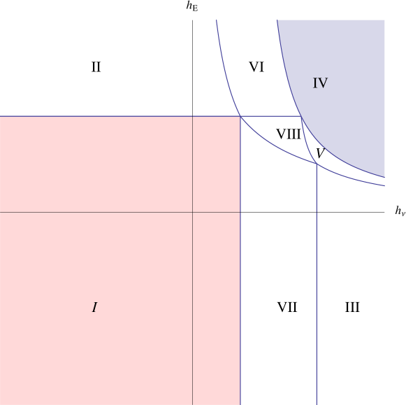
Figure 7.1: Regions for the different lepton mass configurations allowed at the absolute minimum in the $h_{\nu}-h_{E}$ plane for $g<0$ - The different regions correspond to different mass patterns distinct from the quark case, see text and the appendix 10.2 for details.

The possibilities for the vacua have grown sensibly. This is related to the flavour group $\mathcal{G}_{\mathcal{F}}^{l}$ which, in contrast with the quark case, allows for the new invariant at the renormalizable level $I_{R}$. This invariant gives rise to the maximal angle solution and produces new configurations for the values of flavour fields eigenvalues at the minimum. Indeed in the limit $h_{\nu}^{\prime}\rightarrow 0$ all these different cases recombine in the ones for the quark case, see Sec. 10.2 of the appendix.

As for the possible combinations of charged lepton and neutrino eigenvalues scenarios with (at least) two degenerate neutrino masses can come along with hierarchical (case III) or semi-hierarchical (case V) charged lepton spectrum. Lifting the electron mass from 0 is possible in case V via the introduction of small breaking terms of the axial symmetry, giving the lightest lepton a naturally smaller mass.

The general conclusion is therefore that in first approximation a maximal mixing angle is obtained in the lepton sector whereas for the quark case no mixing is allowed in this same level of approximation. This stands as a tantalizing framework for explaining the differences in mixing matrices in the two sectors in a symmetry framework comprising both quarks and leptons. The solution of the maximal angle can be traced back to the presence of an orthogonal group in the flavour symmetry of the lepton sector, which is in turn related to the Majorana nature of neutrino masses.

7.2.3 Realistic mixing and spectrum

The study of flavour symmetry breaking for the quark sector in the bi-fundamental case yielded as a possibility a hierarchical up and down-type fermion spectrum with no mixing, which is a good approximation to the Yukawa couplings to order $\lambda_{c}^{2}$. The lepton case resulted in a possible flavour pattern with a maximal mixing angle, a hierarchical charged lepton spectrum and at least two degenerate neutrinos. Nonetheless even if the neutrino mass spectrum allows for such a situation at present it is the case that the mixing matrix in leptons presents two large angles, so the question arises of whether the present framework can accommodate a second large angle and a good first approximation (at least as good as for quarks) to nature . The present section presents an ansatz to address this question.

The Jacobian analysis pointed to permutation matrices for $\mathcal{U}_{R}\mathcal{U}_{R}^{T}$ as candidates for extremal points, however in the renormalizable potential only the identity and the “antidiagonal” configuration were allowed as absolute minima. Let us postulate that a different permutation matrix can be a local long-lived-enough minimum of the present potential or a minimum of a different, possibly non-renormalizable, potential. We assume furthermore a degenerate neutrino spectrum, and a semihierarchical charged lepton spectrum as in case V, that is,

$$\mathcal{Y}_{E}=\Lambda_{f}\left(\begin{array}[]{ccc}0&0&0\\ 0&y_{\mu}&0\\ 0&0&y_{\tau}\\ \end{array}\right),\qquad\mathcal{Y}_{\nu}=\Lambda_{f}\,y_{\nu}\left(\begin{array}[]{ccc}1&0&0\\ 0&1/\sqrt{2}&-i/\sqrt{2}\\ 0&1/\sqrt{2}&i/\sqrt{2}\\ \end{array}\right),$$ (7.143)

and a neutrino mass matrix,

$$U_{PMNS}\mathbf{m}_{\nu}U_{PMNS}^{T}=\frac{y^{2}v^{2}}{2M}\left(\begin{array}[]{ccc}1&0&0\\ 0&0&1\\ 0&1&0\end{array}\right)\,.$$ (7.144)

In this configuration even if the three neutrinos are degenerate in mass one can tell one of them from the rest from the relative maximal Majorana phase, as previously. The angle among the two completely degenerate neutrino states nonetheless is undetermined at this point such that small perturbations may orient it in an arbitrary direction (126).

As an explicit example let us input the following perturbations to the neutrino matrix, the general case can be found in Sec. 10.3 of the appendix,

$$U_{PMNS}\mathbf{m}_{\nu}U_{PMNS}^{T}=\frac{y^{2}v^{2}}{2M}\left(\begin{array}[]{ccc}1+\delta&(\epsilon+\tilde{\epsilon})/2&(\epsilon-\tilde{\epsilon})/2\\ (\epsilon+\tilde{\epsilon})/2&\delta&1\\ (\epsilon-\tilde{\epsilon})/2&1&\delta\\ \end{array}\right)\,.$$ (7.145)

which lead to the mixing matrix:

$$U_{PMNS}=\left(\begin{array}[]{ccc}\frac{1}{\sqrt{2}}&-\frac{1}{\sqrt{2}}&\frac{\tilde{\epsilon}}{2\sqrt{2}}\\[5.69054pt] \frac{1}{2}+\frac{\tilde{\epsilon}}{4\sqrt{2}}&\frac{1}{2}-\frac{\tilde{\epsilon}}{4\sqrt{2}}&\frac{1}{\sqrt{2}}\\[5.69054pt] -\frac{1}{2}+\frac{\tilde{\epsilon}}{4\sqrt{2}}&-\frac{1}{2}-\frac{\tilde{\epsilon}}{4\sqrt{2}}&\frac{1}{\sqrt{2}}\end{array}\right)\left(\begin{array}[]{ccc}1&0&0\\ 0&1&0\\ 0&0&i\\ \end{array}\right)+\mathcal{O}(\epsilon^{2},...)\,,$$ (7.152)

$$\theta_{12}\simeq\pi/4\,,\qquad\theta_{23}\simeq\pi/4\,,\qquad\theta_{13}\simeq\frac{\tilde{\epsilon}}{2\sqrt{2}}\,.$$ (7.153)

and a mass spectrum, to first order:

$$m_{\nu_{1}}\simeq\frac{y^{2}v^{2}}{2M}\left(1+\delta-\frac{\epsilon}{\sqrt{2}}\right)\,,\quad m_{\nu_{2}}\simeq\frac{y^{2}v^{2}}{2M}\left(1+\delta+\frac{\epsilon}{\sqrt{2}}\right)\,,$$ (7.154)

$$|m_{\nu_{3}}|\simeq\frac{y^{2}v^{2}}{2M}\left(1-\delta\right)\,,$$ (7.155)

which stands as an acceptable first order approximation to the lepton flavour pattern. It is then possible to achieve a first sketch of both quark and lepton flavour patterns with a similar $(\sim\mathcal{O}(10\%))$ approximation. The origin of the perturbations introduced is however yet to be specified consistently and constitutes work in progress.

Finally a phenomenological remark on the fate of this scenario; the degenerate case for neutrino masses is at present very close to the present upper limits of neutrino mass, such that new data from experiments such as neutrinoless double-beta decay may rule out or boost the explanation for flavour here proposed, see (17, 18).

8 Resumen y Conclusiones

En esta tesis la estructura de sabor de las partículas elementales ha sido examinada desde el punto de vista de una posible simetría de sabor implícita. La simetría de sabor considerada es la simetría global que presenta el ME en ausencia de masa para los fermiones. La extensión necesaria del ME para acomodar masas de neutrinos introduce no obstante una dependencia en el modelo elegido. Por simplicidad el escenario del Seesaw con neutrinos pesados (conocido como tipo I) es considerado cuando se trata de leptones, asumiendo la existencia de $n_{g}$ generaciones ligeras y pesadas. La simetría de sabor es entonces seleccionada como la mayor simetría posible de la teoría libre, esquemáticamente  $\mathcal{G_{F}}\sim U(n_{g})^{5}\times O(n_{g})$, en dónde $O(n_{g})$ está asociado a neutrinos pesados degenerados, cuya masa es la única presente en la teoría libre, mientras que cada factor $U(n_{g})$ corresponde a cada campo con distinta carga en el ME.

Sin espicificar un modelo de sabor es posible explorar la posibilidad de que, a bajas energías, los Yukawas sean las fuentes de sabor en el ME y la teoría que lo completa; esta suposición está en acuerdo con los datos experimentales y se encuetra en el centro del éxito fenomenológico de la hipótesis de MFV, implementada a través de técnicas de Lagrangianos efectivos. Prosiguiendo este camino, hemos explorado las consecuencias de un carácter dinámico de los acoplos de Yukawa mediante la determinación, en una base general, de los posibles extremos del conjunto de invariantes (gauge y de sabor) que pueden ser construidos con éstos. Existen tantos invariantes independientes como parámetros físicos, y un conjunto de invariantes completo e independiente ha sido determinado. Los extremos son identificados mediante el estudio del Jacobiano de cambio de base de los parámetros físicos a los invariantes. Hemos demostrado que, mientras para quarks los extremos de los invariantes apuntan hacia la ausencia de mezcla, para leptones grandes ángulos correlacionados con un carácter de Majorana no trivial resultan ser los extremos naturales. En particular, una configuración posible presenta tres neutrinos degenerados, un ángulo atmosférico máximo ($\theta_{23}=\pi/4$) y una fase de Majorana máxima ($\pi/2$). Esta estrutura, al ser perturbada, desarrolla un ángulo solar ($\theta_{12}$) genéricamente grande, dado que esta variable parametriza una dirección plana a primer orden, y un ángulo reactor ($\theta_{13}$) perturbativo. Éste puede ser un motivador y sugerente primer paso en la empresa del entendimiento del origen de sabor, dado que este esquema resulta muy similar al obesrvado en la naturaleza y puede ser testeado en el futuro cercano (17).

Un verdadero origen dinámico de los acoplos de Yukawa sugiere un paso más: considerar que corresponden a campos dinámicos, o agregados de éstos, que poseen sabor y han adquirido un vev. La simetría de sabor sería manifiesta en el Lagrangiano total de alta energía, a una escala $\Lambda_{f}$. Tras la rotura espontánea de simetría, los acoplos de Yukawa de bajas energías resultarían de operadores efectivos de dimension $d>4$ invariantes bajo la simetría de sabor, que involucran uno o mas campos de sabor junto con los campos usuales del ME.

Solo un escalar (o cunjunto de campos en una configuracion escalar) puede tomar un vev, que deberá corresponder al mínimo de un potencial. ¿Cuál es el potencial escalar para estos campos escalares de sabor? ¿Puede alguno de sus mínimos corresponder naturalmente al espectro observado de masas y ángulos? Estas preguntas son respondidas en el presente trabajo. El análisis del potencial está relacionado con los extremos de los invariantes mencionados antes, pero va mas allá dado que el potencial no tiene necesariamente que compartir los puntos extremos del an lisis de los invariantes ni presentar stos como m nimos absolutos del potencial.

La realización mas simple de este tipo se obtene via una correspondencia uno a uno de cada acoplo de Yukawa (up, down, elecrón y neutrino) con un único campo escalar perteneciente a la representación bi-fundamental del grupo de sabor $\mathcal{G_{F}}$. En el lenguaje de Lagrangianos efectivos este caso corresponde al orden más bajo en la expansión de sabor: operadores de Yukawa de dimension $d=5$ construidos por un campo escalar y los campos del ME usuales. El potencial escalar general para campos escalares bi-fundamentales ha sido construido para quarks y leptones en el caso de dos y tres familias. Formalmente, se construye con los invariantes mencionados arriba y no obstante de su combinación surgen nuevos mínimos.

Al determinar el potencial escalar, primero se demostró que imponer la simetría de sabor representa una condición muy restrictiva: al nivel renormalizable sólo ciertos términos son permitidos en el potencial, e incluso al nivel renormalizable estructuras constreñidas deben ser respetadas.

En el caso de quarks, al nivel renormalizable, en el mínimo del potencial solo ángulos nulos son permitidos. Respecto a jerarquías de masa, uno de los posibles mínimos presenta masas nulas para todos los quarks excepto los pertenecientes a la familia más pesada, esto es, un quark tipo down y otro tipo up con masa solamente tanto en dos como en tres familias. Existe por lo tanto una solución incial que se asemeja en primera aproximación a la naturaleza: un espectro jerárquico sin mezcla. Dicha solución puede ser pertubada al nivel renormalizable para obtener masas para las familia más ligera mediante términos de rotura explícita de la parte abeliana de $\mathcal{G_{F}}^{q}$, es decir $U(1)^{3}$. La introducción de términos no renormalizables en el potencial permite una rotura mayor de la simetría, al precio de enormes ajustes finos, que son inaceptables en nuestra opinión en el espíritu de la teoría efectiva de campos.

En el sector leptónico la misma realización de correspondencia Yukawa-campo, escalares bi-fundamentales, condujo a resultados soprendentemente diferentes. En el caso de dos y tres familias, fases de Majorana y ángulos de mezcla no triviales pueden ser seleccionados por el mínimo del potencial, indicando una nueva conexión en la estructura de masas de neutrinos: i) grandes ángulos de mezcla son posibles; ii) hay una fuerte correlación entre ángulos de mezcla grandes y espectro degenerado de masas; iii) la fase de Majorana relativa es predicha como máxima, $2\alpha=\pi/2$, aunque no implica violación de conjugación de carga y paridad observable.

Las soluciones exactas del potencial renomalizable condujentes a mezcla no trivial muestran un único ángulo máximo entre dos neutrinos degenerados pero distinguibles tanto para el caso de dos como el de tres familias. Esto conduce, para el caso de jerarquía normal e invertida, a el ángulo máximo siendo el solar en lugar del atmosférico, numéricamente compatible con un valor máximo. El caso de tres neutrino ligeros degenerados y ángulos de mezcla grandes para $\theta_{12}$ y $\theta_{23}$ identificado en el análisis de extremos de los invariantes no aparece no obstante como mínimo absoluto del potential renormalizable; podría ser un mínimo local de dicho potencial o el mínimo absoluto de un potencial no-renormalizable.

Otra avenida explorada en este trabajo asocia dos campos a cada acoplo de Yukawa, esto es $Y\sim\chi^{L}\chi^{R\dagger}/\Lambda_{f}^{2}$. Esta situación es atrayente dado que mientras que los Yukawas son objetos compuestos, los nuevos campos están en la representación fundamental. Dichos campos podrían ser escalares o fermiónicos: aqui nos centramos exclusivamente en escalares. Desde el punto de vista de Lagrangianos efectivos, este caso podría corresponder al siguiente al primer orden en la expansión: operadores de Yukawa efectivos de dimension 6, como fuentes totales o parciales de los Yukawas de baja energía. Hemos construído el potencial escalar general para campos escalares en la representación fundamental para los casos de dos y tres familias de quarks, aunque las conclusiones se transladan de manera directa a leptones. Por construcción este escenario resulta inevitablemente en una fuerte jerarquía de masas: solamente un quark en cada sector up y down obtiene masa: los quarks top y bottom. Una mezcla no trivial requiere dos campos escalares de sector up y down (neutrino y electrón) transformando bajo el grupo $SU(3)_{Q_{L}}$. En consequencia el contenido mínimo es de cuatro campos $\chi^{L}_{U\,(\nu)}$, $\chi^{L}_{D\,(E)}$, $\chi^{R}_{U\,(\nu)}$ and $\chi^{R}_{D\,(E)}$ y la mezcla surge de la interacción entre los dos primeros. En resumen, para escalares en la fundamental en un modo natural se obtiene: i) una fuerte jerarquía entre quarks de la misma carga, señalando un quark distinguible por su mayor masa en cada sector; ii) un ángulo de mezcla no trivial, que puede ser identificado tanto para quarks como para leptones con el del sector $23$ en el caso de tres familias.

Finalmente, como una posible corrección a los patrones discutidos previamente, se ha discutido brevemente la posibilidad de introducir simultáneamente escalares bi-fundamentales y fundamentales. Es una posibilidad muy sensata, desde el punto de vista de Lagrangianos efectivos, considerar operadores de Yukawa de orden $d=5$ y $d=6$ trabajando a orden $\mathcal{O}(1/\Lambda_{f}^{2})$. Sugiere que el término de $d=5$, que acarrea bi-fundamentales, podría proporcionar la contribución dominante, mientras que el operador de $d=6$, que trae consigo los campos en la fundamental, proporciona correcciones para inducir masas no nulas para las dos familias ligeras junto con ángulos no triviales.

En general, es destacable que el requisito de invarianza bajo la simetría de sabor constriña fuertemente el potencial escalar y consequentemente los mínimos y patrones de ruptura de simetría. De entre los resultados obtenidos uno sobresale de entre los demás. En el mínimo del potencial, al nivel renormalizable, los ángulos de mezcla para quarks son nulos a primer orden, mientras que la mezcla en los leptones resulta ser máxima. La presencia de mezcla máxima es debida al factor $O(n_{g})$ del grupo de sabor, que está a su vez relacionado con la naturaleza Majorana de los neutrinos. La explicación de la diferente estructura de mixing entre quarks y leptones en este escenario es, en última instancia, la distinta naturaleza de los dos tipos de fermiones: Dirac y Majorana.

9 Summary and Conclusions

In this dissertation the flavour pattern of the elementary particles was examined from the point of view of its possible underlying flavour symmetry. The flavour symmetry considered is the global flavour symmetry which the SM possesses in the limit of massless fermions. The necessary extension of the SM to accommodate Majorana neutrino masses introduces nevertheless a model dependence in the neutrino sector; for simplicity the seesaw scenario with heavy right-handed neutrinos (known as type I) is considered here when dealing with leptons, assuming $n_{g}$ generations in both the light and heavy sectors. The largest possible flavour symmetry of the free theory for both quark and lepton sectors is then, schematically,  $\mathcal{G_{F}}\sim U(n_{g})^{5}\times O(n_{g})$, with $O(n_{g})$ associated to heavy degenerate neutrinos, whose mass is the only one present in the free theory, and each $U(n_{g})$ factor for each SM fermion field.

Without particularizing to any concrete flavour model, it is possible to explore the possibility that, at low energies, the Yukawas may be the sources of flavour in the SM and beyond; this assumption is well in agreement with data and lies at the heart of the phenomenological success of the MFV ansatz, implemented through effective Lagrangian techniques. Walking further on this path, we have explored the consequences of an hypothetical dynamical character for the Yukawa couplings themselves by determining, on general grounds, the possible extrema of the (gauge and flavour) invariants that can be constructed out of them. There are as many independent invariants as physical parameters, and a complete set of independent invariants has been determined. The extrema are identified via the study of the Jacobian of the change of basis from the physical parameters to invariants. We have shown that, while for quarks the extrema of the invariants point to no mixing, for leptons maximal mixing angles and Majorana phases correlated with neutrino mass degeneracy turn out to be natural extrema. In particular, a possible configuration presents three degenerate neutrinos, a maximal ($\pi/4$) atmospheric angle ($\theta_{23}$) and a maximal relative Majorana phase ($\pi/2$). This last setup when perturbed presents a generically large solar angle ($\theta_{12}$), since this variable parametrizes a flat direction at first order, and a perturbative reactor angle ($\theta_{13}$) together with small neutrino mass splittings. This may be a very encouraging and suggestive first step in the quest for the understanding of the origin of flavour, as these patterns resemble closely the mixings observed in nature and the degeneracy of neutrino masses will be tested in the near future (17).

A true dynamical origin for the Yukawa couplings suggests a further step: to consider them as corresponding to dynamical fields, or aggregate of fields, that carry flavour and have taken a vev. Flavour would be a manifest symmetry of the total, high energy Lagrangian, at a flavour scale $\Lambda_{f}$. After spontaneous symmetry breaking, the low-energy Yukawa interactions would result from effective operators of dimension $d>4$ invariant under the flavour symmetry, which involve one or more flavour fields together with the usual SM fermionic and Higgs fields.

Only a scalar field (or an aggregate of fields in a scalar configuration) can get a vev, which should correspond to the minimum of a potential. What is the scalar potential for those scalar flavour fields? May some of its minima naturally correspond to the observed spectra of masses and mixing angles? These questions have been addressed in this work. The analysis of the potential is related to the extrema of the invariants mentioned above, but it goes beyond since the potential need neither share the extremal points of the invariant analysis nor present these extremal points as absolute minima.

The simplest realization of this kind is obtained by a one-to-one correspondence of each Yukawa coupling with a single scalar field transforming in the bi-fundamental of the flavour group $\mathcal{G_{F}}$. In the language of effective Lagrangians, this may correspond to the lowest order terms in the flavour expansion: $d=5$ effective Yukawa operators made out of one flavour field plus the usual SM fields. The general scalar potential for bi-fundamental flavor scalar fields was constructed for quark and leptons in the two and three family case. Formally, it can be simply built out of the same Yukawa invariants mentioned above: from their combination new minima may a priori follow.

When determining the scalar potential, it was first shown that the underlying flavour symmetry is a very restrictive constraint: at the renormalizable level only a few terms are allowed in the potential, and even at the non-renormalizable level quite constrained patterns have to be respected.

For the quark case at the renormalizable level, at the minimum of the potential only vanishing mixing angles are allowed. Regarding mass hierarchies, one of the possible minima allows vanishing Yukawa couplings for all quarks but those in the heaviest family, both for the two and three generation cases. There is therefore an starting solution in the quark case which resembles in first approximation nature: a hierarchical spectrum with no mixing. This type of solution can be perturbed at the renormalizable level to provide masses for the lightest family, by means of small explicit breaking terms of the abelian part of $\mathcal{G}_{\mathcal{F}}^{q}$, that is $U(1)^{3}$. The introduction of non-renormalizable terms in the potential allowed for further breaking of the symmetry, at the price of large fine-tunings, which are in our opinion unacceptable in the spirit of and effective field theory approach.

For the lepton sector, the same realization one-Yukawa-one-field, that is, of scalar bi-fundamental fields led to strikingly different results. In the two and three family cases non-trivial Majorana phases and mixing angles may be selected by the potential minima, configurations contained in the invariants extrema analysis. The differences with the quark case are: i) large mixing angles are possible; ii) there is a strong correlation between mixing strength and mass spectrum; iii) the relative Majorana phase among the two massive neutrinos is predicted to be maximal, $2\alpha=\pi/2$, for non-trivial mixing angle; moreover, although the Majorana phase is maximal, it does not lead to experimental signatures of CP violation, as it exists a basis in which all terms in the Lagrangian are real.

The exact solutions of the renormalizable potential leading to non-trivial mixing showed one maximal mixing angle only among two degenerate in mass but distinct (since their relative Majorana phase is maximal) neutrinos for both two and three generations. This scenario leads in the case of normal or inverted hierarchies to the maximal angle being the solar instead of the atmospheric angle. The case of all three neutrinos degenerate, large $\theta_{12}$ and maximal $\theta_{23}$ identified in the invariants extrema analysis turns out not to be present as an absolute minimum of the renormalizable potential; it could be a local minimum of the renormalizable potential or and absolute minimum of a nonrenormalizable potential.

Another avenue explored in this work associates two vector flavour fields to each Yukawa spurion, i.e. a Yukawa $Y\sim\chi^{L}\chi^{R\dagger}/\Lambda_{f}^{2}$. This is an attractive scenario in that while Yukawas are composite objects, the new fields are in the fundamental representation of the flavour group, in analogy with the case of quarks. From the point of view of effective Lagrangians, this case corresponds to $d=6$ effective Yukawa operators.

In a first step we considered the $d=6$ operator contribution alone, such that no $d=5$ operator is present. In this context the general renormalizable scalar potential for scalar flavour fields in the fundamental representation was constructed, both for the case of two and three families of quarks, although conclusions translate straightforwardly to leptons. By construction, this scenario results unavoidably in a strong hierarchy of masses: only one quark gets mass in each sector: the top and bottom quark. Non-trivial mixing requires as expected a misalignment between the flavour fields associated to the up and down (neutrino and electron) left-handed quarks (leptons). In consequence, the minimal field content corresponds to four fields $\chi^{L}_{U\,(\nu)}$, $\chi^{L}_{D\,(E)}$, $\chi^{R}_{U\,(\nu)}$ and $\chi^{R}_{D\,(E)}$, and the physics of mixing lies in the interplay of the first two. In resume, for fundamental flavour fields it follows in a completely natural way: i) a strong mass hierarchy between quarks of the same charge, pointing to a distinctly heavier quark in each sector; ii) one non-vanishing mixing angle, which can be identified with the rotation in the $23$ sector for both quark and leptons in the three generation case.

Finally, as a possible correction to the patterns above, we briefly explored the possibility of introducing simultaneously bi-fundamentals and fundamentals flavour fields. It is a very sensible possibility from the point of view of effective Lagrangians to consider both $d=5$ and $d=6$ Yukawa operators when working to $\mathcal{O}(1/\Lambda_{f}^{2})$. It suggests that $d=5$ operators, which bring in the bi-fundamentals, could give the dominant contributions, while the $d=6$ operator - which brings in the fundamentals - should provide a correction inducing the masses of the two lighter families and non-zero angles.

Overall, it is remarkable that the requirement of invariance under the flavour symmetry strongly constraints the scalar potential. Furthermore, one result of the analysis stands out among the rest. In the minimum of the potential, at the renormalizable level the quark mixing angles vanish at leading order, whereas lepton mixing is found to be maximal. The presence of the maximal angle in the lepton case is due to the $O(n_{g})$ factor of the flavour group, which is in turn related of the Majorana nature of neutrinos. The explanation of the different mixing patterns in quarks and leptons in this scheme is, utterly, the different fundamental nature of the two types of fermions: Dirac and Majorana.

10 Appendix

10.1 $\mathcal{G}_{\mathcal{F}}^{q}$-invariant renormalizable potential formulae of the vevs of $\mathcal{Y}_{D,U}$

In the following the complete vacua configuration of the bi-fundamental quark fields is given in terms of the potential parameters. The only two assumptions are: i) a negative $g$ coefficient ($g<0$), since this yields the approximate observed alignment of up and down sectors, ii) both $I_{U}$ and $I_{D}$ as defined in Eqs. 6.9,6.85 being non-zero at the minimum. The expression for $I_{U,D}$ at the minimum is:

$$\left(\begin{array}[]{c}I_{U}\\ I_{D}\end{array}\right)=\frac{1}{2}(\lambda+\lambda^{\prime})^{-1}\cdot\mu^{2}\,,$$ (10.1)

where $\lambda$ and $\lambda^{\prime}$ are $2\times 2$ real symmetric matrices and $\mu^{2}$ is a real vector in 2 dimensions. Assumption ii) implies that the product $(\lambda+\lambda^{\prime})^{-1}\cdot\mu^{2}$ is a positive 2-vector. $\lambda$ and $\mu^{2}$ are defined in Eq. 6.60 and $\lambda^{\prime}$ differs for each of the vacua configurations detailed in Sec. 6.1.1.2. Each of the different vacua has a distinct breaking pattern: $\mathcal{G}_{\mathcal{F}}^{q}\rightarrow\mathcal{H}^{q}$. The formulae for the different possibilities are given next for $n_{g}$ families where $n_{g}=2,3$ although the results can presumably be extended to any $n_{g}$.

• The unbroken group is $\mathcal{H}^{q}=U(n_{g}-1)^{3}\times U(1)$ and the solution for the field vevs:

  $$\mathcal{Y}_{D}=\Lambda_{f}\mbox{Diag}\left(0\,,\,\cdots\,,\,0\,,\,y_{b}\right)\,,\qquad\mathcal{Y}_{U}=\Lambda_{f}\mbox{Diag}\left(0\,,\,\cdots\,,\,0\,,\,y_{t}\right)\,,$$ (10.2)

  $$\lambda^{\prime}=\left(\begin{array}[]{cc}h_{U}&\frac{g-|g|}{4}\\ \frac{g-|g|}{4}&h_{D}\end{array}\right)\,.$$ (10.3)

• The unbroken group is $\mathcal{H}^{q}=U(n_{g}-1)^{2}\times U(1)$ and the fields:

  $$\mathcal{Y}_{D}=\Lambda_{f}\mbox{Diag}\left(y\,,\,\cdots\,,\,y\,,\,y_{b}\right)\,,\qquad\mathcal{Y}_{U}=\Lambda_{f}\mbox{Diag}\left(0\,,\,\cdots\,,\,0\,,\,y_{t}\right)\,,$$ (10.4)

  $$\quad\frac{y_{b}^{2}-y^{2}}{y_{b}^{2}+(n_{g}-1)y^{2}}=\frac{-g}{2h_{D}}\frac{I_{U}}{I_{D}}\,,\qquad\lambda^{\prime}=\left(\begin{array}[]{cc}h_{U}-\frac{n_{g}-1}{n_{g}}\frac{g^{2}}{4h_{D}}&\frac{g}{2n_{g}}\\ \frac{g}{2n_{g}}&\frac{h_{D}}{n_{g}}\end{array}\right)\,.$$ (10.5)

  This solution requires the right hand side of the first equation in 10.5 to lie between $-1/(n_{g}-1)$ and $1$, if it reaches the upper value the minimum in on the edge of case I, edge depicted by the horizontal line in Fig. 6.2. The other limit of this solution is given by $g^{2}-4h_{U}h_{D}=0$ beyond which the absolute minimum is the degenerate case; it is the line in between II and IV in Fig. 6.2.

• The unbroken group is $\mathcal{H}^{q}=U(n_{g}-1)^{2}\times U(1)$ and the fields:

  $$\mathcal{Y}_{D}=\Lambda_{f}\mbox{Diag}\left(0\,,\,\cdots\,,\,0\,,\,y_{b}\right)\,,\qquad\mathcal{Y}_{U}=\Lambda_{f}\mbox{Diag}\left(y\,,\,\cdots\,,\,y\,,\,y_{t}\right)\,,$$ (10.6)

  $$\frac{y_{t}^{2}-y^{2}}{y_{t}^{2}+(n_{g}-1)y^{2}}=\frac{-g}{2h_{U}}\frac{I_{D}}{I_{U}}\,,\qquad\lambda^{\prime}=\left(\begin{array}[]{cc}\frac{h_{U}}{n_{g}}&\frac{g}{2n_{g}}\\ \frac{g}{2n_{g}}&h_{D}-\frac{n_{g}-1}{n_{g}}\frac{g^{2}}{4h_{U}}\end{array}\right)\,.$$ (10.7)

  The limit in which $-g/(2h_{U})=I_{U}/I_{D}$ signals the end of validity of this solution and the transition of the absolute minimum to case I. This limit is depicted as the vertical line of Fig. 6.2.

• The unbroken group is $\mathcal{H}^{q}=U(n_{g})$ and the fields:

  $$\mathcal{Y}_{D}=\Lambda_{f}\mbox{Diag}\left(y\,,\,\cdots\,,\,y\right)\,,\qquad\mathcal{Y}_{U}=\Lambda_{f}\mbox{Diag}\left(y^{\prime}\,,\,\cdots\,,\,y^{\prime}\right)\,,$$ (10.8)

  $$\lambda^{\prime}=\left(\begin{array}[]{cc}\frac{h_{U}}{n_{g}}&\frac{g}{2n_{g}}\\ \frac{g}{2n_{g}}&\frac{h_{D}}{n_{g}}\end{array}\right)\,.$$ (10.9)

  This is the absolute minimum provided $g^{2}<4h_{U}h_{D}$ with $h_{U}>0,h_{D}>0$, this condition in Fig. 6.2 translates in the allowed region above the curved line.

10.2 $\mathcal{G}_{\mathcal{F}}^{l}$-invariant renormalizable potential formulae of the vevs of $\mathcal{Y}_{E,\nu}$

The renormalizable potential allows for the configurations listed in Sec. 7.2.2 for the vevs of the bi-fundamental fields in the case of $h_{\nu}^{\prime}>0$ whereas in the case of $h_{\nu}^{\prime}<0$ the possibilities are the same as in the quark case. The former case is examined in the following for three families, negative $g$ and the assumption of both invariants $I_{E},I_{\nu}$ taking non-zero vevs given by:

$$\left(\begin{array}[]{c}I_{\nu}\\ I_{E}\end{array}\right)=\frac{1}{2}(\lambda+\lambda^{\prime})^{-1}\mu^{2}\,,$$ (10.10)

where $\lambda$ and $\mu^{2}$ as given in Eq. 7.41 are a $2\times 2$ real symmetric matrix and a 2-vector respectively. $\lambda^{\prime}$ is a $2\times 2$ real symmetric matrix different for each vacuum alignment. Each vacuum configuration is in turn characterized by the remaining unbroken subgroup $\mathcal{H}^{l}$.

• The unbroken group is $\mathcal{H}^{l}=U(2)^{2}\times U(1)$ and the fields:

  $$\mathcal{Y}_{E}=\Lambda_{f}\left(\begin{array}[]{ccc}0&0&0\\ 0&0&0\\ 0&0&y_{\tau}\\ \end{array}\right),\qquad\mathcal{Y}_{\nu}=\Lambda_{f}\left(\begin{array}[]{ccc}0&0&0\\ 0&0&0\\ y_{\nu}/\sqrt{2}&0&iy_{\nu}/\sqrt{2}\\ \end{array}\right),$$ (10.11)

  $$\lambda^{\prime}=\left(\begin{array}[]{cc}h_{\nu}&\frac{g}{2}\\ \frac{g}{2}&h_{E}\end{array}\right)\,.$$ (10.12)

• The unbroken group is $\mathcal{H}^{l}=U(2)\times U(1)$ and the fields:

  $$\mathcal{Y}_{E}=\Lambda_{f}\left(\begin{array}[]{ccc}y&0&0\\ 0&y&0\\ 0&0&y_{\tau}\\ \end{array}\right),\qquad\mathcal{Y}_{\nu}=\Lambda_{f}\left(\begin{array}[]{ccc}0&0&0\\ 0&0&0\\ y_{\nu}/\sqrt{2}&0&iy_{\nu}/\sqrt{2}\\ \end{array}\right),$$ (10.13)

  $$\frac{y_{\tau}^{2}-y^{2}}{y_{\tau}^{2}+2y^{2}}=\frac{-g}{2h_{E}}\frac{I_{\nu}}{I_{E}}\,,\qquad\qquad\lambda^{\prime}=\left(\begin{array}[]{cc}-\frac{g^{2}}{6h_{E}}+h_{\nu}&\frac{g}{6}\\ \frac{g}{6}&\frac{h_{E}}{3}\end{array}\right).$$ (10.14)

  For the negative region of $g$, this configuration turns into that of case I for vanishing $y$, which occurs for $-g/(2h_{E})=I_{E}/I_{\nu}$, a limit depicted as the horizontal line of Fig. 7.1.

• The unbroken group is $\mathcal{H}^{l}=U(2)\times U(1)$ and the fields:

  $$\mathcal{Y}_{E}=\Lambda_{f}\left(\begin{array}[]{ccc}0&0&0\\ 0&0&0\\ 0&0&y_{\tau}\\ \end{array}\right),\qquad\mathcal{Y}_{\nu}=\Lambda_{f}\left(\begin{array}[]{ccc}y_{\nu_{1}}/\sqrt{2}&0&-iy_{\nu_{1}}/\sqrt{2}\\ 0&y_{\nu_{2}}&0\\ y_{\nu_{3}}/\sqrt{2}&0&iy_{\nu_{3}}/\sqrt{2}\\ \end{array}\right),$$ (10.15)

  $$\frac{y_{\nu_{3}}^{2}-y_{\nu_{1}}^{2}}{y_{\nu_{3}}^{2}+y_{\nu_{2}}^{2}+y_{\nu_{1}}^{2}}=\frac{-gI_{E}}{2\left(h_{\nu}-h_{\nu}^{\prime}\right)I_{\nu}}\,,\qquad\frac{y_{\nu_{2}}^{2}-y_{\nu_{1}}^{2}}{y_{\nu_{3}}^{2}+y_{\nu_{2}}^{2}+y_{\nu_{1}}^{2}}=\frac{-gI_{E}h_{\nu}^{\prime}}{2\left(h_{\nu}^{2}-h_{\nu}^{\prime 2}\right)I_{\nu}}\,,$$ (10.16)

  $$\lambda^{\prime}=\left(\begin{array}[]{cc}\frac{1}{3}\left(h_{\nu}+h_{\nu}^{\prime}\right)&\frac{g}{6}\\ \frac{g}{6}&h_{E}-\frac{g^{2}(2h_{\nu}+h_{\nu}^{\prime})}{12\left(h_{\nu}^{2}-\left(h_{\nu}^{\prime}\right){}^{2}\right)}\end{array}\right)\,.$$ (10.17)

  This solution turns into case VII when $y_{\nu_{1}}=0$, a limit drawn as the vertical line to the right in Fig. 7.1.

• The unbroken group is $\mathcal{H}^{l}=SO(3)$ and the fields:

  $$\mathcal{Y}_{E}=\Lambda_{f}\left(\begin{array}[]{ccc}y&0&0\\ 0&y&0\\ 0&0&y\\ \end{array}\right),\qquad\mathcal{Y}_{\nu}=\Lambda_{f}y_{\nu}\left(\begin{array}[]{ccc}1/\sqrt{2}&0&-i/\sqrt{2}\\ 0&1&0\\ 1/\sqrt{2}&0&i/\sqrt{2}\\ \end{array}\right),$$ (10.18)

  $$\lambda^{\prime}=\left(\begin{array}[]{cc}\frac{1}{3}\left(h_{\nu}+h_{\nu}^{\prime}\right)&\frac{g}{6}\\ \frac{g}{6}&\frac{h_{E}}{3}\end{array}\right)\,.$$ (10.19)

  This case is the absolute minima provided $4(h_{\nu}-h_{\nu}^{\prime})h_{E}>g^{2}$ and $h_{E}>0$.

• The unbroken group is $\mathcal{H}^{l}=U(1)^{2}$ and the fields:

  $$\mathcal{Y}_{E}=\Lambda_{f}\left(\begin{array}[]{ccc}0&0&0\\ 0&y_{\mu}&0\\ 0&0&y_{\tau}\\ \end{array}\right),\qquad\mathcal{Y}_{\nu}=\Lambda_{f}\left(\begin{array}[]{ccc}y_{\nu_{1}}/\sqrt{2}&0&-iy_{\nu_{1}}/\sqrt{2}\\ 0&y_{\nu_{2}}&0\\ y_{\nu_{3}}/\sqrt{2}&0&iy_{\nu_{3}}/\sqrt{2}\\ \end{array}\right)\,,$$ (10.20)

  $$\frac{y_{\nu_{3}}^{2}-y_{\nu_{1}}^{2}}{y_{\nu_{3}}^{2}+y_{\nu_{2}}^{2}+y_{\nu_{1}}^{2}}=\frac{-gI_{E}\left(4h_{E}\left(h_{\nu}+h_{\nu}^{\prime}\right)-g^{2}\right)}{2\left(8h_{E}\left(h_{\nu}^{2}-\left(h_{\nu}^{\prime}\right)^{2}\right)-g^{2}\left(2h_{\nu}-h_{\nu}^{\prime}\right)\right)I_{\nu}}\,,$$ (10.21)

  $$\frac{y_{\nu_{2}}^{2}-y_{\nu_{1}}^{2}}{y_{\nu_{3}}^{2}+y_{\nu_{2}}^{2}+y_{\nu_{1}}^{2}}=\frac{-gI_{E}\left(4h_{E}h_{\nu}-g^{2}\right)}{2\left(8h_{E}\left(h_{\nu}^{2}-\left(h_{\nu}^{\prime}\right){}^{2}\right)-g^{2}\left(2h_{\nu}-h_{\nu}^{\prime}\right)\right)I_{\nu}}\,,$$ (10.22)

  $$\frac{y_{\tau}^{2}-y_{\mu}^{2}}{y_{\tau}^{2}+y_{\mu}^{2}}=\frac{g^{2}h_{\nu}^{\prime}}{8h_{E}\left(h_{\nu}^{2}-\left(h_{\nu}^{\prime}\right){}^{2}\right)-g^{2}\left(2h_{\nu}-h_{\nu}^{\prime}\right)}\,,$$ (10.23)

  $$\lambda^{\prime}=\left(\begin{array}[]{cc}\frac{1}{3}\left(h_{\nu}+h_{\nu}^{\prime}\right)&\frac{g}{6}\\ \frac{g}{6}&\frac{2g^{4}+8g^{2}h_{E}\left(-4h_{\nu}+h_{\nu}^{\prime}\right)+96h_{E}^{2}\left(h_{\nu}^{2}-\left(h_{\nu}^{\prime}\right){}^{2}\right)}{24\left(g^{2}\left(-2h_{\nu}+h_{\nu}^{\prime}\right)+8h_{E}\left(h_{\nu}^{2}-\left(h_{\nu}^{\prime}\right){}^{2}\right)\right)}\end{array}\right),$$ (10.24)

  This solution turns into case III for $y_{\mu}=0$ and into case VIII for $y_{\nu_{1}}=0$. This two conditions translated into the potential parameters through the equations above allow to draw the lines in Fig. 7.1 between the respective cases.

• The unbroken group is $\mathcal{H}^{l}=U(1)^{2}$ and the fields:

  $$\mathcal{Y}_{E}=\Lambda_{f}\left(\begin{array}[]{ccc}y_{e}&0&0\\ 0&y_{\mu}&0\\ 0&0&y_{\tau}\\ \end{array}\right),\qquad\mathcal{Y}_{\nu}=\Lambda_{f}\left(\begin{array}[]{ccc}0&0&0\\ 0&y_{\nu_{2}}&0\\ y_{\nu_{3}}/\sqrt{2}&0&iy_{\nu_{3}}/\sqrt{2}\\ \end{array}\right),$$ (10.25)

  $$\frac{y_{\tau}^{2}-y_{e}^{2}}{y_{\tau}^{2}+y_{\mu}^{2}+y_{e}^{2}}=\frac{-gI_{\nu}\left(4h_{E}\left(h_{\nu}+h_{\nu}^{\prime}\right)-g^{2}\right)}{4h_{E}\left(2h_{E}\left(2h_{\nu}+h_{\nu}^{\prime}\right)-g^{2}\right)I_{E}}\,,$$ (10.26)

  $$\frac{y_{\mu}^{2}-y_{e}^{2}}{y_{\tau}^{2}+y_{\mu}^{2}+y_{e}^{2}}=\frac{-gI_{\nu}\left(4h_{E}h_{\nu}-g^{2}\right)}{4h_{E}\left(2h_{E}\left(2h_{\nu}+h_{\nu}^{\prime}\right)-g^{2}\right)I_{E}}\,,$$ (10.27)

  $$\frac{y_{\nu_{3}}^{2}-y_{\nu_{2}}^{2}}{y_{\nu_{3}}^{2}+y_{\nu_{2}}^{2}}=\frac{2h_{E}h_{\nu}^{\prime}}{2h_{E}\left(2h_{\nu}+h_{\nu}^{\prime}\right)-g^{2}}\,,$$ (10.28)

  $$\lambda^{\prime}=\left(\begin{array}[]{cc}-\frac{g^{4}+48h_{E}^{2}h_{\nu}\left(h_{\nu}+h_{\nu}^{\prime}\right)-8g^{2}h_{E}\left(2h_{\nu}+h_{\nu}^{\prime}\right)}{24h_{E}\left(g^{2}-2h_{E}\left(2h_{\nu}+h_{\nu}^{\prime}\right)\right)}&\frac{g}{6}\\ \frac{g}{6}&\frac{h_{E}}{3}\end{array}\right)\,.$$ (10.29)

  This solution in the limit $y_{\mu}=y_{e}$ becomes case II and for $y_{e}=0$ it turns into case VIII. These limits are identified in Eqs. 10.26,10.27 and translated in Fig. 7.1 in the respective lines.

• The unbroken group is $\mathcal{H}^{l}=U(2)\times U(1)^{2}$ and the fields:

  $$\mathcal{Y}_{E}=\Lambda_{f}\left(\begin{array}[]{ccc}0&0&0\\ 0&0&0\\ 0&0&y_{\tau}\\ \end{array}\right),\qquad\mathcal{Y}_{\nu}=\Lambda_{f}\left(\begin{array}[]{ccc}0&0&0\\ 0&y_{\nu_{2}}&0\\ y_{\nu_{3}}/\sqrt{2}&0&iy_{\nu_{3}}/\sqrt{2}\\ \end{array}\right),$$ (10.30)

  $$\frac{y_{\nu_{3}}^{2}-y_{\nu_{2}}^{2}}{y_{\nu_{3}}^{2}+y_{\nu_{2}}^{2}}=\frac{I_{\nu}h_{\nu}^{\prime}-gI_{E}}{\left(2h_{\nu}+h_{\nu}^{\prime}\right)I_{\nu}}\,,$$ (10.31)

  $$\lambda^{\prime}=\left(\begin{array}[]{cc}\frac{h_{\nu}\left(h_{\nu}+h_{\nu}^{\prime}\right)}{2h_{\nu}+h_{\nu}^{\prime}}&\frac{g\left(h_{\nu}+h_{\nu}^{\prime}\right)}{2\left(2h_{\nu}+h_{\nu}^{\prime}\right)}\\ \frac{g\left(h_{\nu}+h_{\nu}^{\prime}\right)}{2\left(2h_{\nu}+h_{\nu}^{\prime}\right)}&\frac{-2g^{2}+8h_{E}\left(2h_{\nu}+h_{\nu}^{\prime}\right)}{8\left(2h_{\nu}+h_{\nu}^{\prime}\right)}\end{array}\right)\,.$$ (10.32)

  This solution connects with the hierarchical case of I for $y_{\nu_{2}}=0$, that is at the vertical line on the left in Fig. 7.1.

• The unbroken group is $\mathcal{H}^{l}=U(1)^{3}$ and the fields:

  $$\mathcal{Y}_{E}=\Lambda_{f}\left(\begin{array}[]{ccc}0&0&0\\ 0&y_{\mu}&0\\ 0&0&y_{\tau}\\ \end{array}\right),\qquad\mathcal{Y}_{\nu}=\Lambda_{f}\left(\begin{array}[]{ccc}0&0&0\\ 0&y_{\nu_{2}}&0\\ y_{\nu_{3}}/\sqrt{2}&0&iy_{\nu_{3}}/\sqrt{2}\\ \end{array}\right),$$ (10.33)

  $$\frac{y_{\tau}^{2}-y_{\mu}^{2}}{y_{\tau}^{2}+y_{\mu}^{2}}=\frac{-gh_{\nu}^{\prime}I_{\nu}}{\left(2h_{E}\left(2h_{\nu}+h_{\nu}^{\prime}\right)-g^{2}\right)I_{E}}\,,$$ (10.34)

  $$\frac{y_{\nu_{3}}^{2}-y_{\nu_{2}}^{2}}{y_{\nu_{3}}^{2}+y_{\nu_{2}}^{2}}=\frac{2h_{E}h_{\nu}^{\prime}}{2h_{E}\left(2h_{\nu}+h_{\nu}^{\prime}\right)-g^{2}}\,,$$ (10.35)

  $$\lambda^{\prime}=\left(\begin{array}[]{cc}\frac{-8h_{E}h_{\nu}^{2}+g^{2}h_{\nu}^{\prime}+2h_{\nu}\left(g^{2}-4h_{E}h_{\nu}^{\prime}\right)}{4\left(g^{2}-2h_{E}\left(2h_{\nu}+h_{\nu}^{\prime}\right)\right)}&\frac{g}{4}\\ \frac{g}{4}&\frac{h_{E}}{2}\end{array}\right)\,.$$ (10.36)

  This solution becomes that of case VII for $y_{\mu}=0$, or equivalently for the RHS of Eq. 10.34 equal to 1.

10.3 Perturbations on a extremal degenerate neutrino matrix

A possibility for an extremal or boundary configuration for the neutrino flavour field $\mathcal{Y}_{\nu}$ (see Sec. 7.2.1) yields the following neutrino matrix, where corrections to the pattern are implemented through $\epsilon_{ij}$,

$$\mathbf{m}_{\nu}=\frac{y^{2}v^{2}}{2M}\left(\begin{array}[]{ccc}1+\epsilon_{11}&\epsilon_{12}&\epsilon_{13}\\ \epsilon_{12}&\epsilon_{22}&1\\ \epsilon_{13}&1&\epsilon_{33}\end{array}\right)\,,$$ (10.37)

such that masses, as defined in Eq. 3.36, read,

$$m_{\nu_{1,2}}=\frac{y^{2}v^{2}}{2M}\left(1+\frac{\epsilon_{22}+2\epsilon_{11}+\epsilon_{33}\mp\sqrt{D^{2}}}{4}\right)+\mathcal{O}(\epsilon^{2})\,,$$ (10.38)

$$m_{\nu_{3}}=\frac{y^{2}v^{2}}{2M}\left(1-\frac{\epsilon_{22}+\epsilon_{33}}{2}\right)+\mathcal{O}(\epsilon^{2})\,,$$ (10.39)

where $D^{2}=\left(\epsilon_{22}+\epsilon_{33}-2\epsilon_{11}\right)^{2}+8\left(\epsilon_{12}+\epsilon_{13}\right)^{2}$ and the mixing matrix,

$$U_{PMNS}=\left(\begin{array}[]{ccc}\cos(\omega)&\sin(\omega)&-i\epsilon^{\prime}\cos(\phi)\\ -\frac{\sin(\omega)-\epsilon^{\prime}\cos(\phi+\omega)}{\sqrt{2}}&\frac{\cos(\omega)+\epsilon^{\prime}\sin(\phi+\omega)}{\sqrt{2}}&i\frac{1-\epsilon^{\prime}\sin(\phi)}{\sqrt{2}}\\ -\frac{\sin(\omega)+\epsilon^{\prime}\cos(\phi+\omega)}{\sqrt{2}}&\frac{\cos(\omega)-\epsilon^{\prime}\sin(\phi+\omega)}{\sqrt{2}}&-i\frac{1+\epsilon^{\prime}\sin(\phi)}{\sqrt{2}}\end{array}\right)\,,$$ (10.43)

$$\tan\omega=\frac{2\sqrt{2}\left(\epsilon_{12}+\epsilon_{13}\right)}{2\epsilon_{11}-\epsilon_{22}-\epsilon_{33}-\sqrt{D^{2}}}\,,\qquad\tan\phi=\frac{\epsilon_{22}-\epsilon_{33}}{\sqrt{2}(\epsilon_{12}-\epsilon_{13})}\,,$$ (10.44)

$$\epsilon^{\prime}=\frac{1}{4}\sqrt{2(\epsilon_{12}-\epsilon_{13})^{2}+(\epsilon_{22}-\epsilon_{33})^{2}}\,.$$ (10.45)

to be compared to Eq. 3.45.

References

- (1) Georges Aad et al. Observation of a new particle in the search for the Standard Model Higgs boson with the ATLAS detector at the LHC. Phys.Lett., B716:1–29, 2012.
- (2) Serguei Chatrchyan et al. Observation of a new boson at a mass of 125 GeV with the CMS experiment at the LHC. Phys.Lett., B716:30–61, 2012.
- (3) Tyler Corbett, O.J.P. Eboli, J. Gonzalez-Fraile, and M.C. Gonzalez-Garcia. Constraining anomalous Higgs interactions. Phys.Rev., D86:075013, 2012.
- (4) Pier Paolo Giardino, Kristjan Kannike, Isabella Masina, Martti Raidal, and Alessandro Strumia. The universal Higgs fit. 2013.
- (5) F. Englert and R. Brout. Broken Symmetry and the Mass of Gauge Vector Mesons. Phys.Rev.Lett., 13:321–323, 1964.
- (6) Peter W. Higgs. Broken Symmetries, Massless Particles and Gauge Fields. Phys.Lett., 12:132–133, 1964.
- (7) Peter W. Higgs. Broken Symmetries and the Masses of Gauge Bosons. Phys.Rev.Lett., 13:508–509, 1964.
- (8) David J.E. Callaway. Triviality Pursuit: Can Elementary Scalar Particles Exist? Phys.Rept., 167:241, 1988.
- (9) Giuseppe Degrassi, Stefano Di Vita, Joan Elias-Miro, Jose R. Espinosa, Gian F. Giudice, et al. Higgs mass and vacuum stability in the Standard Model at NNLO. JHEP, 1208:098, 2012.
- (10) Joan Elias-Miro, Jose R. Espinosa, Gian F. Giudice, Gino Isidori, Antonio Riotto, et al. Higgs mass implications on the stability of the electroweak vacuum. Phys.Lett., B709:222–228, 2012.
- (11) R. Alonso, M.B. Gavela, L. Merlo, S. Rigolin, and J. Yepes. Minimal Flavour Violation with Strong Higgs Dynamics. JHEP, 1206:076, 2012.
- (12) R. Alonso, M.B. Gavela, L. Merlo, S. Rigolin, and J. Yepes. Flavor with a light dynamical ”Higgs particle”. Phys.Rev., D87:055019, 2013.
- (13) R. Alonso, M.B. Gavela, L. Merlo, S. Rigolin, and J. Yepes. The Effective Chiral Lagrangian for a Light Dynamical ’Higgs’. 2012.
- (14) R. Alonso, M. Dhen, M.B. Gavela, and T. Hambye. Muon conversion to electron in nuclei in type-I seesaw models. JHEP, 1301:118, 2013.
- (15) R. Alonso, M. B. Gavela, L. Merlo, and S. Rigolin. On the Scalar Potential of Minimal Flavour Violation. JHEP, 07:012, 2011.
- (16) R. Alonso, M.B. Gavela, D. Hernandez, and L. Merlo. On the Potential of Leptonic Minimal Flavour Violation. Phys.Lett., B715:194–198, 2012.
- (17) R. Alonso, M.B. Gavela, G. Isidori, and L. Maiani. Neutrino Mixing and Masses from a Minimum Principle. 2013.
- (18) R. Alonso, M.B. Gavela, D. Hernandez, L. Merlo, and S. Rigolin. Leptonic Dynamical Yukawa Couplings. 2013.
- (19) N. Cabibbo and L. Maiani. Weak interactions and the breaking of hadron symmetries. Evolution of particle physics, pages 50–80, 1970.
- (20) C. D. Froggatt and Holger Bech Nielsen. Hierarchy of Quark Masses, Cabibbo Angles and CP Violation. Nucl. Phys., B147:277, 1979.
- (21) Howard Georgi. Towards a Grand Unified Theory of Flavor. Nucl.Phys., B156:126, 1979.
- (22) Z.G. Berezhiani. The Weak Mixing Angles in Gauge Models with Horizontal Symmetry: A New Approach to Quark and Lepton Masses. Phys.Lett., B129:99–102, 1983.
- (23) R. Sekhar Chivukula and Howard Georgi. Composite Technicolor Standard Model. Phys. Lett., B188:99, 1987.
- (24) Riccardo Barbieri, G.R. Dvali, and Lawrence J. Hall. Predictions from a U(2) flavor symmetry in supersymmetric theories. Phys.Lett., B377:76–82, 1996.
- (25) Zurab Berezhiani and Anna Rossi. Flavor structure, flavor symmetry and supersymmetry. Nucl.Phys.Proc.Suppl., 101:410–420, 2001.
- (26) G. D’Ambrosio, G. F. Giudice, G. Isidori, and A. Strumia. Minimal Flavour Violation: an Effective Field Theory Approach. Nucl. Phys., B645:155–187, 2002.
- (27) Vincenzo Cirigliano, Benjamin Grinstein, Gino Isidori, and Mark B. Wise. Minimal flavor violation in the lepton sector. Nucl. Phys., B728:121–134, 2005.
- (28) Sacha Davidson and Federica Palorini. Various Definitions of Minimal Flavour Violation for Leptons. Phys. Lett., B642:72–80, 2006.
- (29) Rodrigo Alonso, Gino Isidori, Luca Merlo, Luis Alfredo Munoz, and Enrico Nardi. Minimal Flavour Violation Extensions of the Seesaw. JHEP, 06:037, 2011.
- (30) Riccardo Barbieri, Gino Isidori, Joel Jones-Perez, Paolo Lodone, and David M. Straub. U(2) and Minimal Flavour Violation in Supersymmetry. Eur.Phys.J., C71:1725, 2011.
- (31) Anjan S. Joshipura, Ketan M. Patel, and Sudhir K. Vempati. Type I seesaw mechanism for quasi degenerate neutrinos. Phys.Lett., B690:289–295, 2010.
- (32) Leonard Susskind. Dynamics of Spontaneous Symmetry Breaking in the Weinberg- Salam Theory. Phys. Rev., D20:2619–2625, 1979.
- (33) Savas Dimopoulos and Leonard Susskind. Mass without Scalars. Nucl. Phys., B155:237–252, 1979.
- (34) Savas Dimopoulos and John Preskill. Massless Composites with Massive Constituents. Nucl.Phys., B199:206, 1982.
- (35) David B. Kaplan and Howard Georgi. Breaking by Vacuum Misalignment. Phys.Lett., B136:183, 1984.
- (36) David B. Kaplan, Howard Georgi, and Savas Dimopoulos. Composite Higgs Scalars. Phys. Lett., B136:187, 1984.
- (37) Kaustubh Agashe, Roberto Contino, and Alex Pomarol. The Minimal Composite Higgs Model. Nucl.Phys., B719:165–187, 2005.
- (38) Kaustubh Agashe, Roberto Contino, Leandro Da Rold, and Alex Pomarol. A Custodial Symmetry for Z B Anti-B. Phys. Lett., B641:62–66, 2006.
- (39) Ben Gripaios, Alex Pomarol, Francesco Riva, and Javi Serra. Beyond the Minimal Composite Higgs Model. JHEP, 0904:070, 2009.
- (40) Aneesh Manohar and Howard Georgi. Chiral Quarks and the Nonrelativistic Quark Model. Nucl.Phys., B234:189, 1984.
- (41) H. Georgi. Weak Interactions. http://www.people.fas.harvard.edu/ hgeorgi/.
- (42) Steven Weinberg. Baryon and Lepton Nonconserving Processes. Phys.Rev.Lett., 43:1566–1570, 1979.
- (43) Peter Minkowski. mu –¿ e gamma at a Rate of One Out of 1-Billion Muon Decays? Phys.Lett., B67:421, 1977.
- (44) Murray Gell-Mann, Pierre Ramond, and Richard Slansky. COMPLEX SPINORS AND UNIFIED THEORIES. Conf.Proc., C790927:315–321, 1979.
- (45) Rabindra N. Mohapatra and Goran Senjanovic. Neutrino Mass and Spontaneous Parity Violation. Phys.Rev.Lett., 44:912, 1980.
- (46) M. Magg and C. Wetterich. NEUTRINO MASS PROBLEM AND GAUGE HIERARCHY. Phys.Lett., B94:61, 1980.
- (47) J. Schechter and J.W.F. Valle. Neutrino Masses in SU(2) x U(1) Theories. Phys.Rev., D22:2227, 1980.
- (48) C. Wetterich. Neutrino Masses and the Scale of B-L Violation. Nucl.Phys., B187:343, 1981.
- (49) George Lazarides, Q. Shafi, and C. Wetterich. Proton Lifetime and Fermion Masses in an SO(10) Model. Nucl.Phys., B181:287, 1981.
- (50) Rabindra N. Mohapatra and Goran Senjanovic. Neutrino Masses and Mixings in Gauge Models with Spontaneous Parity Violation. Phys.Rev., D23:165, 1981.
- (51) Robert Foot, H. Lew, X.G. He, and Girish C. Joshi. SEESAW NEUTRINO MASSES INDUCED BY A TRIPLET OF LEPTONS. Z.Phys., C44:441, 1989.
- (52) Ernest Ma. Pathways to naturally small neutrino masses. Phys.Rev.Lett., 81:1171–1174, 1998.
- (53) J. Beringer et al. Review of Particle Physics (RPP). Phys.Rev., D86:010001, 2012.
- (54) M. C. Gonzalez-Garcia, Michele Maltoni, and Jordi Salvado. Updated Global Fit to Three Neutrino Mixing: Status of the Hints of . JHEP, 04:056, 2010.
- (55) Shaun A. Thomas, Filipe B. Abdalla, and Ofer Lahav. Upper Bound of 0.28 eV on Neutrino Masses from the Largest Photometric Redshift Survey. Phys. Rev. Lett., 105:031301, Jul 2010.
- (56) H. Georgi and S.L. Glashow. Unity of All Elementary Particle Forces. Phys.Rev.Lett., 32:438–441, 1974.
- (57) S.L. Glashow, J. Iliopoulos, and L. Maiani. Weak Interactions with Lepton-Hadron Symmetry. Phys.Rev., D2:1285–1292, 1970.
- (58) Sandip Pakvasa and Hirotaka Sugawara. Discrete Symmetry and Cabibbo Angle. Phys.Lett., B73:61, 1978.
- (59) P. F. Harrison, D. H. Perkins, and W. G. Scott. Tri-Bimaximal Mixing and the Neutrino Oscillation Data. Phys. Lett., B530:167, 2002.
- (60) Guido Altarelli and Ferruccio Feruglio. Tri-Bimaximal Neutrino Mixing from Discrete Symmetry in Extra Dimensions. Nucl. Phys., B720:64–88, 2005.
- (61) Guido Altarelli and Ferruccio Feruglio. Tri-Bimaximal Neutrino Mixing, and the Modular Symmetry. Nucl. Phys., B741:215–235, 2006.
- (62) Guido Altarelli, Ferruccio Feruglio, and Yin Lin. Tri-Bimaximal Neutrino Mixing from Orbifolding. Nucl. Phys., B775:31–44, 2007.
- (63) Federica Bazzocchi, Luca Merlo, and Stefano Morisi. Fermion Masses and Mixings in a -Based Model. Nucl. Phys., B816:204–226, 2009.
- (64) Guido Altarelli, Ferruccio Feruglio, and Luca Merlo. Revisiting Bimaximal Neutrino Mixing in a Model with Discrete Symmetry. JHEP, 05:020, 2009.
- (65) J. Kubo, A. Mondragon, M. Mondragon, and E. Rodriguez-Jauregui. The Flavor symmetry. Prog.Theor.Phys., 109:795–807, 2003.
- (66) Ferruccio Feruglio, Claudia Hagedorn, Yin Lin, and Luca Merlo. Tri-Bimaximal Neutrino Mixing and Quark Masses from a Discrete Flavour Symmetry. Nucl. Phys., B775:120–142, 2007.
- (67) Ferruccio Feruglio, Claudia Hagedorn, and Robert Ziegler. S4 and CP in a SUSY Model. 2013.
- (68) Martin Holthausen, Manfred Lindner, and Michael A. Schmidt. CP and Discrete Flavour Symmetries. JHEP, 1304:122, 2013.
- (69) Lisa Randall and Raman Sundrum. A Large mass hierarchy from a small extra dimension. Phys.Rev.Lett., 83:3370–3373, 1999.
- (70) Lisa Randall and Raman Sundrum. An Alternative to compactification. Phys.Rev.Lett., 83:4690–4693, 1999.
- (71) Yuval Grossman and Matthias Neubert. Neutrino masses and mixings in nonfactorizable geometry. Phys.Lett., B474:361–371, 2000.
- (72) Tony Gherghetta and Alex Pomarol. A Warped supersymmetric standard model. Nucl.Phys., B602:3–22, 2001.
- (73) Nima Arkani-Hamed, Savas Dimopoulos, and G.R. Dvali. The Hierarchy problem and new dimensions at a millimeter. Phys.Lett., B429:263–272, 1998.
- (74) Nima Arkani-Hamed and Martin Schmaltz. Hierarchies without symmetries from extra dimensions. Phys.Rev., D61:033005, 2000.
- (75) Eugene A. Mirabelli and Martin Schmaltz. Yukawa hierarchies from split fermions in extra dimensions. Phys.Rev., D61:113011, 2000.
- (76) G.C. Branco, Andre de Gouvea, and M.N. Rebelo. Split fermions in extra dimensions and CP violation. Phys.Lett., B506:115–122, 2001.
- (77) Lawrence J. Hall, Hitoshi Murayama, and Neal Weiner. Neutrino mass anarchy. Phys.Rev.Lett., 84:2572–2575, 2000.
- (78) Andre de Gouvea and Hitoshi Murayama. Statistical test of anarchy. Phys.Lett., B573:94–100, 2003.
- (79) Andre de Gouvea and Hitoshi Murayama. Neutrino Mixing Anarchy: Alive and Kicking. 2012.
- (80) W. Buchmuller and D. Wyler. Effective Lagrangian Analysis of New Interactions and Flavor Conservation. Nucl.Phys., B268:621, 1986.
- (81) B. Grzadkowski, M. Iskrzynski, M. Misiak, and J. Rosiek. Dimension-Six Terms in the Standard Model Lagrangian. JHEP, 1010:085, 2010.
- (82) D. Wyler and L. Wolfenstein. Massless Neutrinos in Left-Right Symmetric Models. Nucl.Phys., B218:205, 1983.
- (83) R.N. Mohapatra and J.W.F. Valle. Neutrino Mass and Baryon Number Nonconservation in Superstring Models. Phys.Rev., D34:1642, 1986.
- (84) G.C. Branco, W. Grimus, and L. Lavoura. THE SEESAW MECHANISM IN THE PRESENCE OF A CONSERVED LEPTON NUMBER. Nucl.Phys., B312:492, 1989.
- (85) Martti Raidal, Alessandro Strumia, and Krzysztof Turzynski. Low-scale standard supersymmetric leptogenesis. Phys.Lett., B609:351–359, 2005.
- (86) M.B. Gavela, T. Hambye, D. Hernandez, and P. Hernandez. Minimal Flavour Seesaw Models. JHEP, 0909:038, 2009.
- (87) A. Broncano, M.B. Gavela, and Elizabeth Ellen Jenkins. The Effective Lagrangian for the seesaw model of neutrino mass and leptogenesis. Phys.Lett., B552:177–184, 2003.
- (88) S. Antusch, C. Biggio, E. Fernandez-Martinez, M.B. Gavela, and J. Lopez-Pavon. Unitarity of the Leptonic Mixing Matrix. JHEP, 0610:084, 2006.
- (89) Victor Mukhamedovich Abazov et al. Evidence for an anomalous like-sign dimuon charge asymmetry. Phys.Rev., D82:032001, 2010.
- (90) R. Aaij et al. Evidence for CP violation in time-integrated decay rates. Phys.Rev.Lett., 108:111602, 2012.
- (91) A. Aguilar-Arevalo et al. Evidence for neutrino oscillations from the observation of anti-neutrino(electron) appearance in a anti-neutrino(muon) beam. Phys.Rev., D64:112007, 2001.
- (92) Gino Isidori. Flavor physics and CP violation. 2013.
- (93) J. Adam et al. New constraint on the existence of the mu+ e+ gamma decay. 2013.
- (94) C. Dohmen et al. Test of lepton flavor conservation in mu – e conversion on titanium. Phys.Lett., B317:631–636, 1993.
- (95) Gino Isidori and David M. Straub. Minimal Flavour Violation and Beyond. Eur.Phys.J., C72:2103, 2012.
- (96) L. Michel and L. A. Radicati. Breaking of the symmetry in hadronic physics. Evolution of particle physics, pages 191–203, 1970.
- (97) L. Michel and L.A. Radicati. Properties of the breaking of hadronic internal symmetry. Annals Phys., 66:758–783, 1971.
- (98) Z. Berezhiani and F. Nesti. Supersymmetric SO(10) for fermion masses and mixings: Rank-1 structures of flavor. JHEP, 0603:041, 2006.
- (99) Elizabeth Ellen Jenkins and Aneesh V. Manohar. Algebraic Structure of Lepton and Quark Flavor Invariants and CP Violation. JHEP, 0910:094, 2009.
- (100) Amihay Hanany, Elizabeth E. Jenkins, Aneesh V. Manohar, and Giuseppe Torri. Hilbert Series for Flavor Invariants of the Standard Model. JHEP, 1103:096, 2011.
- (101) Gianluca Blankenburg, Gino Isidori, and Joel Jones-Perez. Neutrino Masses and LFV from Minimal Breaking of and flavor Symmetries. Eur.Phys.J., C72:2126, 2012.
- (102) Thorsten Feldmann, Martin Jung, and Thomas Mannel. Sequential Flavour Symmetry Breaking. Phys. Rev., D80:033003, 2009.
- (103) Enrico Nardi. Naturally large Yukawa hierarchies. Phys.Rev., D84:036008, 2011.
- (104) Jose R. Espinosa, Chee Sheng Fong, and Enrico Nardi. Yukawa hierarchies from spontaneous breaking of the flavour symmetry? JHEP, 1302:137, 2013.
- (105) Benjamin Grinstein, Michele Redi, and Giovanni Villadoro. Low Scale Flavor Gauge Symmetries. JHEP, 1011:067, 2010.
- (106) Thorsten Feldmann. See-Saw Masses for Quarks and Leptons in . JHEP, 04:043, 2011.
- (107) Diego Guadagnoli, Rabindra N. Mohapatra, and Ilmo Sung. Gauged Flavor Group with Left-Right Symmetry. JHEP, 1104:093, 2011.
- (108) Laura Lopez-Honorez and Luca Merlo. Dark matter within the minimal flavour violation ansatz. Phys.Lett., B722:135–143, 2013.
- (109) Andrzej J. Buras, Maria Valentina Carlucci, Luca Merlo, and Emmanuel Stamou. Phenomenology of a Gauged Flavour Model. JHEP, 1203:088, 2012.
- (110) Luciano Maiani. Universality of the Weak Interactions, Cabibbo theory and where they led us. Rivista del Nuovo Cimento, 34,, 679, 2011.
- (111) Alexander L. Kagan, Gilad Perez, Tomer Volansky, and Jure Zupan. General Minimal Flavor Violation. Phys. Rev., D80:076002, 2009.
- (112) F. P. An et al. Observation of Electron-Antineutrino Disappearance at Daya Bay. 2012.
- (113) J.K. Ahn et al. Observation of Reactor Electron Antineutrino Disappearance in the RENO Experiment. Phys.Rev.Lett., 108:191802, 2012.
- (114) Silvia Pascoli and Thomas Schwetz. Prospects for neutrino oscillation physics. Adv.High Energy Phys., 2013:503401, 2013.
- (115) M. De Gerone. Latest results from the MEG experiment. Nucl.Phys.Proc.Suppl., 233:231–236, 2012.
- (116) A. Blondel, A. Bravar, M. Pohl, S. Bachmann, N. Berger, et al. Research Proposal for an Experiment to Search for the Decay eee. 2013.
- (117) Ed V. Hungerford. COMET/PRISM muon to electron conversion at J-PARC. AIP Conf.Proc., 1182:694–697, 2009.
- (118) R. M. Carey et al. [Mu2e Collaboration]. Proposal to search for mu- N -¿ e- N with a single event sensitivity below 10 -16. FERMILAB-PROPOSAL-0973.
- (119) P.A.R. Ade et al. Planck 2013 results. XVI. Cosmological parameters. 2013.
- (120) J.J. Gomez-Cadenas, J. Martin-Albo, M. Mezzetto, F. Monrabal, and M. Sorel. The Search for neutrinoless double beta decay. Riv.Nuovo Cim., 35:29–98, 2012.
- (121) Rodrigo Alonso, Stefan Antusch, Mattias Blennow, Pilar Coloma, Andre de Gouvea, et al. Summary report of MINSIS workshop in Madrid. 2010.
- (122) O.J.P. Eboli, J. Gonzalez-Fraile, and M.C. Gonzalez-Garcia. Neutrino Masses at LHC: Minimal Lepton Flavour Violation in Type-III See-saw. JHEP, 1112:009, 2011.
- (123) D.N. Dinh, A. Ibarra, E. Molinaro, and S.T. Petcov. The mu - e Conversion in Nuclei, mu - e gamma, mu - 3e Decays and TeV Scale See-Saw Scenarios of Neutrino Mass Generation. JHEP, 1208:125, 2012.
- (124) D. Aristizabal Sierra, A. Degee, and J.F. Kamenik. Minimal Lepton Flavor Violating Realizations of Minimal Seesaw Models. JHEP, 1207:135, 2012.
- (125) J.A. Casas and A. Ibarra. Oscillating neutrinos and muon – e, gamma. Nucl.Phys., B618:171–204, 2001.
- (126) Guido Altarelli and Ferruccio Feruglio. Models of neutrino masses and mixings. New J.Phys., 6:106, 2004.