Decuplet baryon masses in covariant baryon chiral perturbation theory

Abstract

We present an analysis of the lowest-lying decuplet baryon masses in the covariant baryon chiral perturbation theory with the extended-on-mass-shell scheme up to next-to-next-to-next-to-leading order. In order to determine the $14$ low-energy constants, we perform a simultaneous fit of the $n_{f}=2+1$ lattice QCD data from the PACS-CS, QCDSF-UKQCD, and HSC Collaborations, taking finite-volume corrections into account self-consistently. We show that up to next-to-next-to-next-to-leading order one can achieve a good description of the lattice QCD and experimental data. Surprisingly, we note that the current lattice decuplet baryon masses can be fitted rather well by the next-to-leading order baryon chiral perturbation theory, which, however, misses the experimental data a little bit. Furthermore, we predict the pion- and strangeness-sigma terms of the decuplet baryons by use of the Feynman-Hellmann theorem.

I Introduction

In the past few years many studies of the lowest-lying baryon octet and decuplet masses have been performed on the lattice Durr et al. (2008); Alexandrou et al. (2009); Aoki et al. (2009, 2010); Walker-Loud et al. (2009); Lin et al. (2009); Bietenholz et al. (2010, 2011); Beane et al. (2011) [see Ref. Fodor and Hoelbling (2012) for a comprehensive discussion of the various lattice chromodynamics (LQCD) simulations and the origin of their uncertainties]. These studies not only demonstrate the ability of LQCD simulations to predict accurately nonperturbative observables of the strong interactions, but also provide valuable information that can be used to extract the low-energy constants (LECs) of chiral perturbation theory (ChPT). On the other hand, most LQCD calculations, limited by the availability of computational resources and the efficiency of algorithms Beringer et al. (2012), still have to employ larger than physical light-quark masses $m_{u/d}$,  finite lattice volume $V=TL^{3}$, and finite lattice spacing $a$. ChPT Weinberg (1979); Gasser and Leutwyler (1984, 1985); Gasser et al. (1988); Leutwyler (1994); Bernard et al. (1995); Pich (1995); Ecker (1995); Pich (1998); Bernard and Meissner (2007); Bernard (2008); Scherer and Schindler (2012) plays an important role in guiding the necessary extrapolations to the physical world in terms of light-quark masses Leinweber et al. (2004); Bernard et al. (2004); Procura et al. (2004); Bernard et al. (2005), lattice volume Ali Khan et al. (2004); Beane (2004) and lattice spacing Beane and Savage (2003); Arndt and Tiburzi (2004), and in estimating the induced uncertainties.

As an effective field theory of low-energy QCD, ChPT has been rather successful in the mesonic sector, but the extension to the one-baryon sector turns out to be nontrivial. Because the baryon mass is not zero in the chiral limit, a systematic power counting is absent Gasser et al. (1988). In order to restore the chiral power counting, the so-called heavy-baryon (HB) ChPT was first proposed by Jenkins and Manohar Jenkins and Manohar (1991). Although this approach provides a strict power counting, the heavy baryon expansion is nonrelativistic. A naive application can lead to pathologies, e.g., in the calculation of the scalar form factor of the nucleon Bernard et al. (1995).  In addition, the HB ChPT is found to converge rather slowly in the three-flavor sector of $u$, $d$, and $s$ quarks. Later, covariant baryon chiral perturbation theory (BChPT) implementing a consistent power counting with different renormalization methods has been developed, such as the infrared (IR) Becher and Leutwyler (1999) and the extended-on-mass-shell (EOMS) Gegelia and Japaridze (1999); Fuchs et al. (2003) renormalization schemes.

In the past decades, the ground-state octet baryon masses have been studied rather extensively Jenkins (1992); Bernard et al. (1993); Banerjee and Milana (1995); Borasoy and Meissner (1997); Walker-Loud (2005); Ellis and Torikoshi (2000); Frink and Meissner (2004); Frink et al. (2005); Lehnhart et al. (2005); Semke and Lutz (2006, 2007); Martin Camalich et al. (2010); Geng et al. (2011); Young and Thomas (2010); Semke and Lutz (2012a, b); Lutz and Semke (2012); Bruns et al. (2013); Ren et al. (2012, 2013), especially, in combination with the $n_{f}=2+1$ LQCD data up to next-to-next-to-next-to-leading order (N³LO) Young and Thomas (2010); Martin Camalich et al. (2010); Geng et al. (2011); Semke and Lutz (2012a, b); Lutz and Semke (2012); Bruns et al. (2013); Ren et al. (2012, 2013). Different formulations of BChPT have been explored, including the HB ChPT Young and Thomas (2010), the EOMS BChPT Martin Camalich et al. (2010); Geng et al. (2011); Ren et al. (2012, 2013), the partial summation approach Semke and Lutz (2012a, b); Lutz and Semke (2012), and the IR BChPT Bruns et al. (2013). In Refs. Martin Camalich et al. (2010); Geng et al. (2011); Ren et al. (2012, 2013), we have performed a series of studies on the octet baryon masses by including finite-volume corrections (FVCs) self-consistently in the EOMS BChPT up to next-to-next-to-leading order (NNLO) and N³LO. In these studies, we found that the N³LO EOMS BChPT can provide a good description of all the current LQCD data for the octet baryon masses, and we confirmed that the LQCD results are consistent with each other, although their setups are different. Furthermore, the FVCs to the LQCD data are found to be important not only for the purpose of chiral extrapolations, but also for the determination of the corresponding LECs, especially for the many LECs appearing at N³LO.

On the contrary, there are only a few studies of the $n_{f}=2+1$ LQCD decuplet baryon masses Walker-Loud et al. (2009); Ishikawa et al. (2009); Semke and Lutz (2012a, b); Lutz and Semke (2012). In Refs. Walker-Loud et al. (2009); Ishikawa et al. (2009), it was shown that the HB ChPT at NNLO cannot describe the LHPC and PACS-CS octet and decuplet baryon masses. This has motivated the series of studies on the $n_{f}=2+1$ LQCD octet baryon masses in the EOMS framework Martin Camalich et al. (2010); Geng et al. (2011); Ren et al. (2012, 2013). The PACS-CS and LHPC decuplet baryon data were also studied in Ref. Martin Camalich et al. (2010) up to NNLO and a reasonable description of the LQCD data was achieved, contrary to the HB ChPT studies of Refs. Walker-Loud et al. (2009); Ishikawa et al. (2009). In Ref. Semke and Lutz (2012a), Semke and Lutz studied the BMW Durr et al. (2008) LQCD data for the octet and decuplet baryon masses up to N³LO in BChPT with the partial summation scheme. It was shown that the light-quark mass dependence of the decuplet baryon masses can be well described. However, FVCs to the lattice data are not taken into account self-consistently. Whereas it has been shown in Refs. Geng et al. (2011); Ren et al. (2012, 2013) that FVCs need to be taken into account self-consistently in order to achieve a $\chi^{2}/\mathrm{d.o.f.}$ of about 1 in the description of the current $n_{f}=2+1$ LQCD octet baryon masses.

Given the fact that a simultaneous description of the $n_{f}=2+1$ LQCD decuplet baryon masses with FVCs taken into account self-consistently is still missing and that the EOMS BChPT can describe the LQCD octet baryon masses rather well Martin Camalich et al. (2010); Geng et al. (2011); Ren et al. (2012, 2013), it is timely to perform a thorough study of the lowest-lying decuplet baryon masses in the EOMS BChPT up to N³LO. The paper is organized as follows: In Sec. II, we collect the relevant chiral effective Lagrangians, which contain $14$ to be determined LECs, and calculate the decuplet baryon masses and the corresponding FVCs in covariant BChPT up to N³LO. In Sec. III, we perform a simultaneous fit of the PACS-CS, QCDSF-UKQCD, and HSC data, study the convergence of BChPT and the contributions of virtual octet and decuplet baryons, and compare the N³LO BChPT with those LQCD data not included in the fit. We then predict the pion- and strangeness-baryon sigma terms with the LECs determined from the best fits and compare them with the results of other recent studies. A short summary is given in Sec. IV.

II Theoretical Framework

II.1 Chiral effective Lagrangians

The chiral effective Lagrangians relevant to the present study can be written as the sum of a mesonic part and a meson-baryon part:

$$\mathcal{L}_{\rm eff}=\mathcal{L}_{\phi}^{(2)}+\mathcal{L}_{\phi}^{(4)}+\mathcal{L}_{\phi D}^{(1)}+\mathcal{L}_{\phi D}^{(2)}+\mathcal{L}_{\phi D}^{(4)}.$$ (1)

The Lagrangians $\mathcal{L}_{\phi}^{(2)}$ and $\mathcal{L}_{\phi}^{(4)}$ of the mesonic sector can be found in Ref. Ren et al. (2012). The leading order meson-baryon Lagrangian is

$$\mathcal{L}_{\phi D}^{(1)}=\mathcal{L}_{D}+\mathcal{L}_{\phi BD}^{(1)}+\mathcal{L}_{\phi DD}^{(1)},$$ (2)

where $\mathcal{L}_{D}$ denotes the covariant free Lagrangian, and $\mathcal{L}_{\phi BD}^{(1)}$ and $\mathcal{L}_{\phi DD}^{(1)}$ describe the interaction of the octet and decuplet baryons with the pseudoscalar mesons and have the following form:

$$\mathcal{L}_{D} = \bar{T}_{\mu}^{abc}\left(i\gamma^{\mu\nu\alpha}D_{\alpha}-m_{D}\gamma^{\mu\nu}\right)T_{\nu}^{abc},$$ (3)

$$\mathcal{L}_{\phi BD}^{(1)} = \frac{i\mathcal{C}}{m_{D}F_{\phi}}\varepsilon^{abc}(\partial_{\alpha}\bar{T}_{\mu}^{ade})\gamma^{\alpha\mu\nu}B_{c}^{e}\partial_{\nu}\phi_{b}^{d}+{\rm H.c.},$$ (4)

$$\mathcal{L}_{\phi DD}^{(1)} = \frac{i\mathcal{H}}{m_{D}F_{\phi}}\bar{T}_{\mu}^{abc}\gamma^{\mu\nu\rho\sigma}\gamma_{5}\left(\partial_{\rho}T_{\nu}^{abd}\right)\partial_{\sigma}\phi_{d}^{c},$$ (5)

where we have used the so-called “consistent” coupling scheme for the meson-octet-decuplet vertices Pascalutsa (1998); Pascalutsa and Timmermans (1999). In the above Lagrangians, $m_{D}$ is the decuplet baryon mass in the chiral limit and $T$ is the decuplet baryon field represented by the Rarita-Schwinger field $T^{abc}\equiv T_{\mu}^{abc}$. The physical fields are assigned as $T^{111}=\Delta^{++}$, $T^{112}=\Delta^{+}/\sqrt{3}$, $T^{122}=\Delta^{0}/\sqrt{3}$, $T^{222}=\Delta^{-}$, $T^{113}=\Sigma^{*+}/\sqrt{3}$, $T^{123}=\Sigma^{*0}/\sqrt{6}$, $T^{223}=\Sigma^{*-}/\sqrt{3}$, $T^{133}=\Xi^{*0}/\sqrt{3}$, $T^{233}=\Xi^{*-}/\sqrt{3}$, and $T^{333}=\Omega^{-}$. $D_{\nu}T_{\mu}^{abc}=\partial_{\nu}T_{\mu}^{abc}+(\Gamma_{\nu},T_{\mu})^{abc}$, $\Gamma_{\nu}=\frac{1}{2}\left\{u^{{\dagger}}\partial_{\nu}u+u\partial_{\nu}u^{{\dagger}}\right\}$ being the chiral connection with $u={\rm exp}\left(i\frac{\phi}{2F_{\phi}}\right)$ collecting the pseudoscalar fields $\phi$, and $(X,T_{\mu})^{abc}\equiv(X)^{a}_{d}T_{\mu}^{dbc}+(X)^{b}_{d}T_{\mu}^{adc}+(X)^{c}_{d}T_{\mu}^{abd}$. The coefficient $F_{\phi}$ is the meson-decay constant in the chiral limit, and $\mathcal{C}$ ($\mathcal{H}$) denotes the $\phi BD$ ($\phi DD$) coupling. The totally antisymmetric gamma matrix products are defined as $\gamma^{\mu\nu}=\frac{1}{2}[\gamma^{\mu},\gamma^{\nu}]$, $\gamma^{\mu\nu\rho}=\frac{1}{2}\{\gamma^{\mu\nu},\gamma^{\rho}\}=-i\varepsilon^{\mu\nu\rho\sigma}\gamma_{\sigma}\gamma_{5}$, $\gamma^{\mu\nu\rho\sigma}=\frac{1}{2}[\gamma^{\mu\nu\rho},\gamma^{\sigma}]=i\varepsilon^{\mu\nu\rho\sigma}\gamma_{5}$ with the following conventions: $g^{\mu\nu}=\mathrm{diag}(1,-1,-1,-1)$, $\varepsilon_{0,1,2,3}=-\varepsilon^{0,1,2,3}=1$, $\gamma_{5}=i\gamma_{0}\gamma_{1}\gamma_{2}\gamma_{3}$ Geng et al. (2008a). In the last and following Lagrangians, we sum over any repeated SU(3) index denoted by latin characters $a$, $b$, $c$, $\ldots$, and $(X)_{b}^{a}$ denotes the element of row $a$ and column $b$ of the matrix representation of $X$.

The meson-baryon Lagrangian at order $\mathcal{O}(p^{2})$ can be written as

$$\mathcal{L}_{\phi D}^{(2)}=\mathcal{L}_{\phi B}^{(2,~{}{\rm sb})}+\mathcal{L}_{\phi D}^{(2,~{}{\rm sb})}+{\mathcal{L}_{\phi D}^{(2)}}^{\prime}.$$ (6)

The first and second terms denote the explicit chiral symmetry breaking part:

$$\mathcal{L}_{\phi B}^{(2,~{}{\rm sb})} = b_{0}\langle\bar{B}B\rangle\langle\chi_{+}\rangle+b_{D/F}\langle\bar{B}\left[\chi_{+},B\right]_{\pm}\rangle,$$ (7)

$$\mathcal{L}_{\phi D}^{(2,~{}{\rm sb})} = \frac{t_{0}}{2}\bar{T}_{\mu}^{abc}g^{\mu\nu}T_{\nu}^{abc}\langle\chi_{+}\rangle+\frac{t_{D}}{2}\bar{T}_{\mu}^{abc}g^{\mu\nu}(\chi_{+},T_{\nu})^{abc},$$ (8)

where $b_{0}$, $b_{D}$, $b_{F}$, $t_{0}$, and $t_{D}$ are the LECs, $\chi_{+}=u^{{\dagger}}\chi u^{{\dagger}}+u\chi^{{\dagger}}u$ , and $\chi=2B_{0}\mathcal{M}$ accounts for explicit chiral symmetry breaking with $B_{0}=-\langle 0|\bar{q}q|0\rangle/F_{\phi}^{2}$ and $\mathcal{M}={\rm diag}(m_{l},~{}m_{l},~{}m_{s})$. For the chiral symmetry conserving part ${\mathcal{L}_{\phi D}^{(2)}}^{\prime}$, one has nine terms, following the conventions of Refs. Lutz and Semke (2011); Semke and Lutz (2012a),

$${\mathcal{L}_{\phi D}^{(2)}}^{\prime} = \frac{1}{F_{\phi}^{2}}\left\{t_{1}\bar{T}_{\mu}^{abc}g^{\mu\nu}\left(\partial^{\sigma}\phi\partial_{\sigma}\phi\right)_{c}^{d}T_{\nu}^{abd}+t_{2}\bar{T}_{\mu}^{abc}\left[\left(\partial^{\mu}\phi\partial_{\nu}\phi\right)_{c}^{d}+\left(\partial_{\nu}\phi\partial^{\mu}\phi\right)_{c}^{d}\right]T^{\nu,abd}\right.$$ (9)

$$+t_{3}\bar{T}_{\mu,abc}\partial_{\nu}\phi_{d}^{a}\varepsilon^{bde}T^{\mu,fgc}\partial^{\nu}\phi_{f}^{h}\varepsilon_{ghe}+t_{4}\bar{T}_{\mu,abc}\left[\partial^{\mu}\phi_{d}^{a}\varepsilon^{bde}\partial_{\nu}\phi_{f}^{h}\varepsilon_{ghe}+\partial_{\nu}\phi_{d}^{a}\varepsilon^{bde}\partial^{\mu}\phi_{f}^{h}\varepsilon_{ghe}\right]T^{\nu,fgc}$$

$$+t_{5}\bar{T}_{\mu}^{abc}g^{\mu\nu}T_{\nu}^{abc}\langle\partial^{\sigma}\phi\partial_{\sigma}\phi\rangle+t_{6}\bar{T}_{\mu}^{abc}T^{\nu,abc}\langle\partial^{\mu}\phi\partial_{\nu}\phi\rangle$$

$$+t_{7}\left[\left(\bar{T}_{\alpha}^{abc}\left(\partial_{\mu}\phi\partial_{\nu}\phi\right)_{c}^{d}i\gamma^{\mu}\partial^{\nu}T^{\alpha,abd}+\bar{T}_{\alpha}^{abc}\left(\partial_{\nu}\phi\partial_{\mu}\phi\right)_{c}^{d}i\gamma^{\mu}\partial^{\nu}T^{\alpha,abd}\right)+{\rm H.c.}\right]$$

$$+t_{8}\left[\left(\bar{T}_{\alpha,abc}\partial_{\mu}\phi_{d}^{a}\varepsilon^{bde}i\gamma^{\mu}\partial^{\nu}T^{\alpha,fgc}\partial_{\nu}\phi_{f}^{h}\varepsilon_{ghe}+\bar{T}_{\alpha,abc}\partial_{\nu}\phi_{d}^{a}\varepsilon^{bde}i\gamma^{\mu}\partial^{\nu}T^{\alpha,fgc}\partial_{\mu}\phi_{f}^{h}\varepsilon_{ghe}\right)+{\rm H.c.}\right]$$

$$\left.+t_{9}\left[\bar{T}_{\alpha}^{abc}i\gamma^{\mu}\partial^{\nu}T^{\alpha,abc}\langle\partial_{\mu}\phi\partial_{\nu}\phi\rangle+{\rm H.c.}\right]\right\},$$

where $t_{1,\dots,6}$ have dimension mass^-1 and $t_{7,\dots,9}$ have dimension mass^-2.

The fourth order chiral effective Lagrangians contain five LECs (see also Refs. Tiburzi and Walker-Loud (2005); Semke and Lutz (2012a)):

$$\mathcal{L}_{\phi D}^{(4)} = e_{1}\bar{T}_{\mu}^{abc}g^{\mu\nu}\left(\chi_{+}^{2}\right)_{d}^{c}T_{\nu}^{abd}+e_{2}\left(\bar{T}_{\mu}^{abc}\left(\chi_{+}\right)_{c}^{d}\right)g^{\mu\nu}\left(\left(\chi_{+}\right)_{e}^{b}T_{\nu}^{aed}\right)$$ (10)

$$+e_{3}\bar{T}_{\mu}^{abc}g^{\mu\nu}\left(\chi_{+}\right)_{d}^{c}T_{\nu}^{abd}\langle\chi_{+}\rangle+e_{4}\bar{T}_{\mu}^{abc}g^{\mu\nu}T_{\nu}^{abc}\langle\chi_{+}\rangle^{2}$$

$$+e_{5}\bar{T}_{\mu}^{abc}g^{\mu\nu}T_{\nu}^{abc}\langle\chi_{+}^{2}\rangle.$$

The propagator of the spin-$3/2$ fields in $d$ dimensions has the following form Pascalutsa and Vanderhaeghen (2006):

$$S^{\mu\nu}(p)=-\frac{\not{p}+m_{D}}{p^{2}-m_{D}^{2}+i\epsilon}\left[g^{\mu\nu}-\frac{1}{d-1}\gamma^{\mu}\gamma^{\nu}-\frac{1}{(d-1)m_{D}}\left(\gamma^{\mu}p^{\nu}-\gamma^{\nu}p^{\mu}\right)-\frac{d-2}{(d-1)m_{D}^{2}}p^{\mu}p^{\nu}\right].$$ (11)

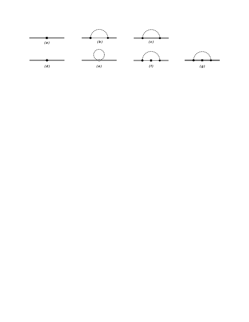
Figure 1: Feynman diagrams contributing to the decuplet baryon masses up to $\mathcal{O}(p^{4})$ in the EOMS BChPT. The single lines correspond to octet baryons, double lines to decuplet baryons and dashed lines to mesons. The black boxes (diamond) indicate second (fourth) order couplings. The solid dot (circle-cross) indicates an insertion from the dimension one (two) meson-baryon Lagrangians. Wave function renormalization diagrams are not explicitly shown but included in the calculation.

II.2 Decuplet baryon masses

In this subsection, the decuplet baryon masses are calculated in the limit of exact isospin symmetry. Formally, up to $\mathcal{O}(p^{4})$ the baryon masses can be written as

$$M_{D}=m_{D}+m_{D}^{(2)}+m_{D}^{(3)}+m_{D}^{(4)},$$ (12)

where $m_{D}$ is the decuplet baryon mass in the chiral limit. The $m_{D}^{(2)}$, $m_{D}^{(3)}$, and $m_{D}^{(4)}$ are the next-to-leading order (NLO), NNLO, and N³LO chiral corrections to the decuplet baryon masses, respectively. The corresponding Feynman diagrams are shown in Fig. 1, and the explicit expression of the decuplet baryon masses is

$$M_{D} = m_{D}+\xi_{D,\pi}^{(a)}M_{\pi}^{2}+\xi_{D,K}^{(a)}M_{K}^{2}$$ (13)

$$+\frac{1}{(4\pi F_{\phi})^{2}}\sum\limits_{\phi=\pi,~{}K,~{}\eta}\left[\xi_{D,\phi}^{(b)}H_{D}^{(b)}(M_{\phi})+\xi_{D,\phi}^{(c)}H_{D}^{(c)}(M_{\phi})\right]$$

$$+\xi_{D,\pi}^{(d)}M_{\pi}^{4}+\xi_{D,K}^{(d)}M_{K}^{4}+\xi_{D,\pi K}^{(d)}M_{\pi}^{2}M_{K}^{2}$$

$$+\frac{1}{(4\pi F_{\phi})^{2}}\sum\limits_{\phi=\pi,~{}K,~{}\eta}\left[\xi_{D,\phi}^{(e,1)}H_{D}^{(e,1)}(M_{\phi})+\xi_{D,\phi}^{(e,2)}H_{D}^{(e,2)}(M_{\phi})+\xi_{D,\phi}^{(e,3)}H_{D}^{(e,3)}(M_{\phi})\right]$$

$$-\frac{1}{(4\pi F_{\phi})^{2}}\sum_{\begin{subarray}{c}\phi=\pi,~{}K,~{}\eta\\ B=N,~{}\Lambda,~{}\Sigma,~{}\Xi\end{subarray}}\xi_{DB,\phi}^{(f)}H_{D,B}^{(f)}(M_{\phi})$$

$$-\frac{1}{(4\pi F_{\phi})^{2}}\sum_{\begin{subarray}{c}\phi=\pi,~{}K,~{}\eta\\ D^{\prime}=\Delta,~{}\Sigma^{*},~{}\Xi^{*},~{}\Omega^{-}\end{subarray}}\xi_{DD^{\prime},\phi}^{(g)}H_{D,D^{\prime}}^{(g)}(M_{\phi}),$$

where $\xi^{(i)}$’s and $H^{(i)}$’s are the corresponding coefficients and loop functions with the subscript $i$ denoting the corresponding diagrams shown in Fig. 1. The $\xi^{(i)}$’s are tabulated in Tables 1 and 2.

Table 1: Coefficients of the NLO and NNLO contributions to the decuplet baryon masses [Eq. (13)].

	$\Delta$	$\Sigma^{*}$	$\Xi^{*}$	$\Omega^{-}$
$\xi_{D,\pi}^{(a)}$	$t_{0}+3t_{D}$	$t_{0}+t_{D}$	$t_{0}-t_{D}$	$t_{0}-3t_{D}$
$\xi_{D,K}^{(a)}$	$2t_{0}$	$2t_{0}+2t_{D}$	$2t_{0}+4t_{D}$	$2t_{0}+6t_{D}$
$\xi_{D,\pi}^{(b)}$	$\frac{4}{3}\mathcal{C}^{2}$	$\frac{10}{9}\mathcal{C}^{2}$	$\frac{2}{3}\mathcal{C}^{2}$	$0$
$\xi_{D,K}^{(b)}$	$\frac{4}{3}\mathcal{C}^{2}$	$\frac{8}{9}\mathcal{C}^{2}$	$\frac{4}{3}\mathcal{C}^{2}$	$\frac{8}{3}\mathcal{C}^{2}$
$\xi_{D,\eta}^{(b)}$	$0$	$\frac{2}{3}\mathcal{C}^{2}$	$\frac{2}{3}\mathcal{C}^{2}$	$0$
$\xi_{D,\pi}^{(c)}$	$\frac{50}{27}\mathcal{H}^{2}$	$\frac{80}{81}\mathcal{H}^{2}$	$\frac{10}{27}\mathcal{H}^{2}$	$0$
$\xi_{D,K}^{(c)}$	$\frac{20}{27}\mathcal{H}^{2}$	$\frac{160}{81}\mathcal{H}^{2}$	$\frac{20}{9}\mathcal{H}^{2}$	$\frac{40}{27}\mathcal{H}^{2}$
$\xi_{D,\eta}^{(c)}$	$\frac{10}{27}\mathcal{H}^{2}$	$0$	$\frac{10}{27}\mathcal{H}^{2}$	$\frac{40}{27}\mathcal{H}^{2}$

Table 2: Coefficients of the N³LO contributions to the decuplet baryon masses [Eq. (13)], with the following notations: $\tilde{t}_{1}=2t_{1}+t_{2}$, $\tilde{t}_{2}=2t_{3}+t_{4}$, and $\tilde{t}_{3}=4t_{5}+t_{6}$.

	$\Delta$	$\Sigma^{*}$	$\Xi^{*}$	$\Omega^{-}$
$\xi_{D,\pi}^{(d)}$	$4(e_{1}+e_{2}+e_{3}+e_{4}+3e_{5})$	$\frac{4}{3}(3e_{1}-e_{2}+e_{3}+3e_{4}+9e_{5})$	$\frac{4}{3}(3e_{1}-e_{2}-e_{3}+3e_{4}+9e_{5})$	$4(e_{1}+e_{2}-e_{3}+e_{4}+3e_{5})$
$\xi_{D,K}^{(d)}$	$16(e_{4}+e_{5})$	$\frac{16}{3}(e_{1}+e_{3}+3e_{4}+3e_{5})$	$\frac{16}{3}(2e_{1}+e_{2}+2e_{3}+3e_{4}+3e_{5})$	$16(e_{1}+e_{2}+e_{3}+e_{4}+e_{5})$
$\xi_{D,\pi K}^{(d)}$	$8(e_{3}+2e_{4}-2e_{5})$	$-\frac{16}{3}(e_{1}-e_{2}-e_{3}-3e_{4}+3e_{5})$	$-\frac{8}{3}(4e_{1}-e_{3}-6e_{4}+6e_{5})$	$-16(e_{1}+e_{2}-e_{4}+e_{5})$
$\xi_{D,\pi}^{(e,1)}$	$\frac{3}{2}(2t_{0}+3t_{D})M_{\pi}^{2}$	$3(t_{0}+t_{D})M_{\pi}^{2}$	$\frac{3}{2}(2t_{0}+t_{D})M_{\pi}^{2}$	$3t_{0}M_{\pi}^{2}$
$\xi_{D,K}^{(e,1)}$	$(4t_{0}+3t_{D})M_{K}^{2}$	$4(t_{0}+t_{D})M_{K}^{2}$	$(4t_{0}+5t_{D})M_{K}^{2}$	$2(2t_{0}+3t_{D})M_{K}^{2}$
$\xi_{D,\eta}^{(e,1)}$	$\frac{1}{6}\left[8t_{0}M_{K}^{2}-(2t_{0}-3t_{D})M_{\pi}^{2}\right]$	$\frac{1}{3}(t_{0}+t_{D})(4M_{K}^{2}-M_{\pi}^{2})$	$\frac{1}{6}\left[8(t_{0}+2t_{D})M_{K}^{2}-(2t_{0}+7t_{D})M_{\pi}^{2}\right]$	$\frac{1}{3}\left[4(t_{0}+3t_{D})M_{K}^{2}-(t_{0}+6t_{D})M_{\pi}^{2}\right]$
$\xi_{D,\pi}^{(e,2)}$	$-\frac{1}{2}(3\tilde{t}_{1}+2\tilde{t}_{2}+3\tilde{t}_{3})$	$-\frac{1}{6}(6\tilde{t}_{1}+5\tilde{t}_{2}+9\tilde{t}_{3})$	$-\frac{1}{2}(\tilde{t}_{1}+\tilde{t}_{2}+3\tilde{t}_{3})$	$-\frac{3}{2}\tilde{t}_{3}$
$\xi_{D,K}^{(e,2)}$	$-(\tilde{t}_{1}+\tilde{t}_{2}+2\tilde{t}_{3})$	$-\frac{2}{3}(2\tilde{t}_{1}+\tilde{t}_{2}+3\tilde{t}_{3})$	$-\frac{1}{3}(5\tilde{t}_{1}+3\tilde{t}_{2}+6\tilde{t}_{3})$	$-2(\tilde{t}_{1}+\tilde{t}_{2}+\tilde{t}_{3})$
$\xi_{D,\eta}^{(e,2)}$	$-\frac{1}{6}(\tilde{t}_{1}+3\tilde{t}_{3})$	$-\frac{1}{6}(2\tilde{t}_{1}+3\tilde{t}_{2}+3\tilde{t}_{3})$	$-\frac{1}{2}(\tilde{t}_{1}+\tilde{t}_{2}+\tilde{t}_{3})$	$-\frac{1}{6}(4\tilde{t}_{1}+3\tilde{t}_{3})$
$\xi_{D,\pi}^{(e,3)}$	$-4(3t_{7}+2t_{8}+3t_{9})$	$-\frac{4}{3}(6t_{7}+5t_{8}+9t_{9})$	$-4(t_{7}+t_{8}+3t_{9})$	$-12t_{9}$
$\xi_{D,K}^{(e,3)}$	$-8(t_{7}+t_{8}+2t_{9})$	$-\frac{16}{3}(2t_{7}+t_{8}+3t_{9})$	$-\frac{8}{3}(5t_{7}+3t_{8}+6t_{9})$	$-16(t_{7}+t_{8}+t_{9})$
$\xi_{D,\eta}^{(e,3)}$	$-\frac{4}{3}(t_{7}+3t_{9})$	$-\frac{4}{3}(2t_{7}+3t_{8}+3t_{9})$	$-4(t_{7}+t_{8}+t_{9})$	$-\frac{4}{3}(4t_{7}+3t_{9})$
$\xi_{DN,\{\pi,K,\eta\}}^{(f)}$	$\{2\mathcal{C}^{2},0,0\}$	$\{0,\frac{2}{3}\mathcal{C}^{2},0\}$	$\{0,0,0\}$	$\{0,0,0\}$
$\xi_{D\Lambda,\{\pi,K,\eta\}}^{(f)}$	$\{0,0,0\}$	$\{\mathcal{C}^{2},0,0\}$	$\{0,\mathcal{C}^{2},0\}$	$\{0,0,0\}$
$\xi_{D\Sigma,\{\pi,K,\eta\}}^{(f)}$	$\{0,2\mathcal{C}^{2},0\}$	$\{\frac{2}{3}\mathcal{C}^{2},0,\mathcal{C}^{2}\}$	$\{0,\mathcal{C}^{2},0\}$	$\{0,0,0\}$
$\xi_{D\Xi,\{\pi,K,\eta\}}^{(f)}$	$\{0,0,0\}$	$\{0,\frac{2}{3}\mathcal{C}^{2},0\}$	$\{\mathcal{C}^{2},0,\mathcal{C}^{2}\}$	$\{0,0,4\mathcal{C}^{2}\}$
$\xi_{D\Delta,\{\pi,K,\eta\}}^{(g)}$	$\{\frac{5}{3}\mathcal{H}^{2},0,\frac{1}{3}\mathcal{H}^{2}\}$	$\{0,\frac{8}{9}\mathcal{H}^{2},0\}$	$\{0,0,0\}$	$\{0,0,0\}$
$\xi_{D\Sigma^{*},\{\pi,K,\eta\}}^{(g)}$	$\{0,\frac{2}{3}\mathcal{H}^{2},0\}$	$\{\frac{8}{9}\mathcal{H}^{2},0,0\}$	$\{0,\frac{4}{3}\mathcal{H}^{2},0\}$	$\{0,0,0\}$
$\xi_{D\Xi^{*},\{\pi,K,\eta\}}^{(g)}$	$\{0,0,0\}$	$\{0,\frac{8}{9}\mathcal{H}^{2},0\}$	$\{\frac{1}{3}\mathcal{H}^{2},0,\frac{1}{3}\mathcal{H}^{2}\}$	$\{0,\frac{4}{3}\mathcal{H}^{2},0\}$
$\xi_{D\Omega^{-},\{\pi,K,\eta\}}^{(g)}$	$\{0,0,0\}$	$\{0,0,0\}$	$\{0,\frac{2}{3}\mathcal{H}^{2},0\}$	$\{0,0,\frac{4}{3}\mathcal{H}^{2}\}$

In Eq. (13), the loop functions $H_{D}^{(b)}$, $H_{D}^{(c)}$, $H_{D}^{(e,1)}$, $H_{D}^{(e,2)}$, $H_{D}^{(e,3)}$, $H_{D,B}^{(f)}$, and $H_{D,D^{\prime}}^{(g)}$ are obtained by using the $\overline{\rm MS}$ renormalization scheme to remove the divergent pieces and the EOMS renormalization scheme to remove the power-counting-breaking (PCB) terms Gegelia and Japaridze (1999); Fuchs et al. (2003); Geng (2013). The explicit expressions of $H_{D}^{(b)}$, $H_{D}^{(c)}$ can be found in Ref. Martin Camalich et al. (2010), and the others are given in the Appendix.

It should be noted that in the evaluation of the diagrams in Figs. 1(f) and (g), we have only kept terms linear in $M_{D}^{(2)}$ and $M_{B}^{(2)}$, in accordance with our power counting. At N³LO, the pseudoscalar meson masses appearing in $m_{D}^{(2)}$ should be replaced by their $\mathcal{O}(p^{4})$ counterparts to generate the N³LO contributions to $m_{D}^{(4)}$. The explicit expressions of the meson masses up to $\mathcal{O}(p^{4})$ can be found in Ref. Gasser and Leutwyler (1985). The empirical values of the LECs $L_{i}^{r}$ $(i=1,\dots,10)$ are taken from the latest global fit Bijnens and Jemos (2012). In order to be consistent with our renormalization scale used for the baryon sector, we have reevaluated the LECs at $\mu=1$ GeV. The details can be found in Ref. Ren et al. (2012). 

II.3 Finite-volume corrections

As emphasized in Refs. Geng et al. (2011); Ren et al. (2012, 2013), FVCs have to be taken into account in studying the current LQCD data. In the case of the decuplet baryon masses, they have been studied up to NNLO in the EOMS BChPT Martin Camalich et al. (2010) and in the HB ChPT Ishikawa et al. (2009). In the following, we extend the study up to N³LO in the EOMS BChPT.

The FVCs can be easily evaluated following the standard technique. One chooses the baryon rest frame, i.e., $p^{\mu}=(m_{D},\vec{0})$, performs a momentum shift and wick rotation, integrates over the temporal dimension, and obtains the results expressed in terms of the master formulas given in Ref. Beane (2004). See Refs.Ali Khan et al. (2004); Beane (2004); Geng et al. (2011) for more details.

To proceed with the above procedure, one should note that since Lorentz invariance is lost in finite volume, the mass term in the loop functions is identified as the term having the structure of $\delta_{ij}$. This can be easily seen by noticing that at the rest frame the zero component of the decuplet baryon field vanishes because of the on-shell condition $p_{\mu}T^{\mu}=0$. For instance, the loop function of the diagram in Fig. 1(b), after Feynman parametrization, becomes

$$G^{(b)}_{D}\propto\int\frac{d^{4}k}{(2\pi)^{4}}\frac{(m_{D}(x-1)-m_{B})k^{\alpha}k^{\beta}}{\left(k^{2}-{\mathcal{M}_{D}^{(b)}}^{2}\right)^{2}},$$ (14)

where ${\mathcal{M}_{D}^{(b)}}^{2}=(x^{2}-x)m_{D}^{2}+xm_{0}^{2}+(1-x)M_{\phi}^{2}-i\epsilon$. To evaluate its contribution to the decuplet baryon mass, one simply replaces $k^{\alpha}k^{\beta}$ with $\delta_{ij}\vec{k}^{2}/3$ in the numerator. Following the procedure specified above, one can then easily obtain the FVCs to the loop function of the diagram in Fig. 1(b),

$$\delta G_{D}^{(b)}(M_{\phi}) \equiv G_{D}^{(b)}(L)-G_{D}^{(b)}(\infty)$$ (15)

$$= -\frac{1}{12}\int_{0}^{1}dx~{}\left[m_{0}-m_{D}(x-1)\right]\left[\delta_{1/2}({\mathcal{M}_{D}^{(b)}}^{2})-{\mathcal{M}_{D}^{(b)}}^{2}\delta_{3/2}({\mathcal{M}_{D}^{(b)}}^{2})\right],$$

where the “master” formulas $\delta_{r}(\mathcal{M}^{2})$ are defined as

$$\delta_{r}(\mathcal{M}^{2})=\frac{2^{-1/2-r}(\sqrt{\mathcal{M}^{2}})^{3-2r}}{\pi^{3/2}\Gamma(r)}\sum_{\vec{n}\neq 0}(L\sqrt{\mathcal{M}^{2}}|\vec{n}|)^{-3/2+r}K_{3/2-r}(L\sqrt{\mathcal{M}^{2}}|\vec{n}|),$$ (16)

where $K_{n}(z)$ is the modified Bessel function of the second kind, and $\sum\limits_{\vec{n}\neq 0}\equiv\sum\limits^{\infty}_{n_{x}=-\infty}\sum\limits^{\infty}_{n_{y}=-\infty}\sum\limits^{\infty}_{n_{z}=-\infty}(1-\delta(|\vec{n}|,0))$ with $\vec{n}=(n_{x},n_{y},n_{z})$.

Following the same procedure, one can obtain the FVCs of the other loop diagrams in Fig. 1. For the NNLO one-loop diagram of Fig. 1(c), one obtains

$$\delta G_{D}^{(c)}(M_{\phi})=\frac{5}{36}\int_{0}^{1}dx~{}m_{D}(x-2)\left[\delta_{1/2}({\mathcal{M}_{D}^{(c)}}^{2})-{\mathcal{M}_{D}^{(c)}}^{2}\delta_{3/2}({\mathcal{M}_{D}^{(c)}}^{2})\right],$$ (17)

with ${\mathcal{M}_{D}^{(c)}}^{2}=x^{2}m_{D}^{2}+(1-x)M_{\phi}^{2}-i\epsilon.$ Taking the limit of $m_{D}\rightarrow\infty$, Eq. (15) and Eq. (17) reduce to

$$\delta G_{D}^{(b)}(M_{\phi})_{\rm HB} = -\frac{1}{8}\int_{0}^{\infty}dx\left[\delta_{1/2}(\beta_{\Delta}^{2})-\beta_{\Delta}^{2}\delta_{3/2}(\beta_{\Delta}^{2})\right],$$ (18)

$$\delta G_{D}^{(c)}(M_{\phi})_{\rm HB} = \frac{1}{2}\int_{0}^{\infty}dx\left[\delta_{1/2}(\beta^{2})-\beta^{2}\delta_{3/2}(\beta^{2})\right],$$ (19)

where $\beta_{\Delta}=x^{2}-2x\delta+M_{\phi}^{2}$ and $\beta=x^{2}+M_{\phi}^{2}$. They agree with the HB ChPT results of Ref. Ishikawa et al. (2009).

FVCs to the N³LO one-loop diagrams in Figs. 1 (e), (f), and (g) have the following form:

$$\delta G_{D}^{(e,1)}(M_{\phi}) = \frac{1}{2}\delta_{1/2}(M_{\phi}^{2}),$$ (20)

$$\delta G_{D}^{(e,2)}(M_{\phi}) = \frac{1}{2}M_{\phi}^{2}\delta_{1/2}(M_{\phi}^{2}),$$ (21)

$$\delta G_{D}^{(e,3)}(M_{\phi}) = \frac{1}{2}m_{D}\delta_{-1/2}(M_{\phi}^{2}),$$ (22)

$$\delta G_{D,B}^{(f)}(M_{\phi}) = \frac{1}{12}\int_{0}^{1}dx\left\{\left[m_{D}^{(2)}(x-1)-m_{B}^{(2)}\right]\cdot\delta_{1/2}({\mathcal{M}_{D}^{(b)}}^{2})\right.$$ (23)

$$+\left[(1-x)\left(2{\mathcal{M}_{D}^{(b)}}^{2}+M_{\phi}^{2}(x-1)-(m_{0}+m_{D})(m_{0}+2m_{D})x+2m_{D}^{2}x^{2}\right)m_{D}^{(2)}\right.$$

$$\quad+\left.\left({\mathcal{M}_{D}^{(b)}}^{2}+3m_{0}x(m_{0}+m_{D}(1-x))\right)m_{B}^{(2)}\right]\cdot\delta_{3/2}({\mathcal{M}_{D}^{(b)}}^{2})$$

$$+{\mathcal{M}_{D}^{(b)}}^{2}\left[(x-1)\left({\mathcal{M}_{D}^{(b)}}^{2}+M_{\phi}^{2}(x-1)-(m_{0}+m_{D})(m_{0}+2m_{D})x+2m_{D}^{2}x^{2}\right)m_{D}^{(2)}\right.$$

$$\left.\left.\quad-3m_{0}x(m_{0}+m_{D}(1-x))m_{B}^{(2)}\right]\cdot\delta_{5/2}({\mathcal{M}_{D}^{(b)}}^{2})\right\},$$

$$\delta G_{D,D^{\prime}}^{(g)}(M_{\phi}) = \frac{5}{36}\int_{0}^{1}dx\left\{\left[(3x-5)m_{D}^{(2)}+(3-2x)m_{D^{\prime}}^{(2)}\right]\cdot\delta_{1/2}({\mathcal{M}_{D}^{(c)}}^{2})\right.$$ (24)

$$+\left[\left({\mathcal{M}_{D}^{(c)}}^{2}(10-6x)+2m_{D}^{2}x(2x-3)+M_{\phi}^{2}(-3x^{2}+8x-5)\right)m_{D}^{(2)}\right.$$

$$\quad+\left.\left({\mathcal{M}_{D}^{(c)}}^{2}(2x-3)-3m_{D}^{2}(x^{2}-2x)\right)m_{D^{\prime}}^{(2)}\right]\cdot\delta_{3/2}({\mathcal{M}_{D}^{(c)}}^{2})$$

$$+\left[{\mathcal{M}_{D}^{(c)}}^{2}\left(m_{D}^{2}(6x-4x^{2})+{\mathcal{M}_{D}^{(c)}}^{2}(3x-5)+M_{\phi}^{2}(x-1)(3x-5)\right)m_{D}^{(2)}\right.$$

$$\quad+\left.\left.3{\mathcal{M}_{D}^{(c)}}^{2}m_{D}^{2}(x^{2}-2x)m_{D^{\prime}}^{(2)}\right]\cdot\delta_{5/2}({\mathcal{M}_{D}^{(c)}}^{2})\right\}.$$

The above standard procedure applies only to the case where $m_{D}\leq m_{0}+M_{\phi}$. For the case of $m_{D}>m_{0}+M_{\phi}$, we follow the approach proposed in Ref. Bernard et al. (2008) and replace the original $\delta_{r}(\mathcal{M}^{2})$ with three parts by introducing a new scale $\mu$ satisfying $\mu<m_{0}+M_{\phi}$, i.e.,

$$\delta_{r}(\mathcal{M}^{2})=g_{1}^{r}-g_{2}^{r}+g_{3}^{r},$$ (25)

where the $g_{1,2,3}^{r}$ are defined as

$$g_{1}^{r} = \frac{1}{L^{3}}\sum\limits_{\vec{k}}\left\{\frac{1}{\left[\frac{4\pi^{2}\vec{n}^{2}}{L^{2}}+\mathcal{M}^{2}(m_{D}^{2})\right]^{r}}-\frac{1}{\left[\frac{4\pi^{2}\vec{n}^{2}}{L^{2}}+\mathcal{M}^{2}(\mu^{2})\right]^{r}}+\frac{r(x^{2}-x)(m_{D}^{2}-\mu^{2})}{\left[\frac{4\pi^{2}\vec{n}^{2}}{L^{2}}+\mathcal{M}^{2}(\mu^{2})\right]^{r+1}}\right\},$$ (26)

$$g_{2}^{r} = \int_{0}^{+\infty}\frac{k^{2}dk}{2\pi^{2}}\cdot\left\{\frac{1}{\left[\vec{k}^{2}+\mathcal{M}^{2}(m_{D}^{2})\right]^{r}}-\frac{1}{\left[\vec{k}^{2}+\mathcal{M}^{2}(\mu^{2})\right]^{r}}+\frac{r(x^{2}-x)(m_{D}^{2}-\mu^{2})}{\left[\vec{k}^{2}+\mathcal{M}^{2}(\mu^{2})\right]^{r+1}}\right\},$$ (27)

$$g_{3}^{r} = \delta_{r}\left(\mathcal{M}^{2}(\mu^{2})\right)-r(x^{2}-x)(m_{D}^{2}-\mu^{2})\delta_{r+1}\left(\mathcal{M}^{2}(\mu^{2})\right),$$ (28)

with

$$\mathcal{M}^{2}(m_{D}^{2}) = (x^{2}-x)m_{D}^{2}+xm_{0}^{2}+(1-x)M_{\phi}^{2}-i\epsilon,$$ (29)

$$\mathcal{M}^{2}(\mu^{2}) = (x^{2}-x)\mu^{2}+xm_{0}^{2}+(1-x)M_{\phi}^{2}-i\epsilon.$$ (30)

To take into account the FVCs in the study of the LQCD data, one simply replaces the loop functions $H$ of Eq. (13) by $\tilde{H}=H+\delta G$ with the $\delta G$s calculated above.

III Results and discussion

In this section, we perform a simultaneous fit of the $n_{f}=2+1$ LQCD data from the PACS-CS Aoki et al. (2009), QCDSF-UKQCD Bietenholz et al. (2011), and HSC Lin et al. (2009) Collaborations and the experimental data Beringer et al. (2012) to determine the $17$ unknown LECs, $m_{D}$, $t_{D}$, $t_{0\cdots 9}$, and $e_{1\cdots 5}$. Since $t_{1}$, $t_{2}$, $t_{3}$, $t_{4}$, $t_{5}$, and $t_{6}$ appear in combinations, effectively we have only 14 independent LECs. The pion or light-quark mass dependence of the decuplet baryon masses is studied in the NLO, NNLO, and N³LO EOMS BChPT. Using the so-obtained LECs, we also carry out a detailed study on the QCDSF-UKQCD and LHPC data to test the applicability of the N³LO BChPT and the consistency between different LQCD simulations. Furthermore, the pion- and strangeness-baryon sigma terms are predicted by the use of the Feynman-Hellmann theorem.

III.1 LQCD data and values of LECs

Up to now, five collaborations have reported $n_{f}=2+1$ simulations of the decuplet baryon masses, i.e., the BMW Durr et al. (2008), PACS-CS Aoki et al. (2009), LHPC Walker-Loud et al. (2009), HSC Lin et al. (2009), and QCDSF-UKQCD Bietenholz et al. (2011) Collaborations. Because the BMW data are not publicly available and the data of the LHPC Collaboration seem to suffer some systematic errors, as shown in their chiral extrapolation result on the $\Delta$(1232) mass, which is much higher than its physical value Walker-Loud et al. (2009) (see also Sec. III.2), we will concentrate on the data of the PACS-CS, QCDSF-UKQCD, and HSC Collaborations. Following the criteria used in our previous studies Ren et al. (2013), we only select the LQCD data that satisfy $M_{\pi}<0.5$ GeV and $M_{\phi}L>3.8$. As a result, there are eight sets of data from the PACS-CS (3 sets), QCDSF-UKQCD (2 sets), and HSC (3 sets) Collaborations. Among the eight LQCD data sets studied, only in the ensemble with $M_{\pi}=296$ MeV from the PACS-CS Collaboration, can the decay $\Delta\rightarrow N+\pi$ happen. It should be noted that the PACS-CS Collaboration measured the lowest energy levels of the vector meson and decuplet baryon channels, which are different from the true resonance masses. The resulting difference for the $\rho$ meson is estimated to be 5 percent using Lüscher’s formula Aoki et al. (2009). We will comment on this later.

It should be mentioned that the $\mathcal{O}(a)$-improved Wilson action was used by all the above collaborations except the LHPC Collaboration, which employed a mixed action. The $\mathcal{O}(a)$-improved action has the favorable property that the leading order corrections from the finite lattice spacing are eliminated. The finite lattice spacing corrections of the mixed action of the LHPC Collaboration were also shown to be small Walker-Loud et al. (2009). Therefore, in the present work we assume that the discretization artifacts of the present LQCD simulations are small and can be ignored, and will leave a detailed study on finite lattice spacing artifacts to a future study (for a recent study of the discretization effects on the octet baryon masses, see Ref. Ren et al. (2014)).

Before we perform a simultaneous fit of the LQCD data, we specify our strategy to fix some of the LECs in the N³LO BChPT mass formulas [Eq. (13)]. For the meson-decay constant, we use $F_{\phi}=0.0871$ GeV. The $\phi BD$ coupling is fixed to the SU(3)-average value among the different decuplet-to-octet pionic decay channels, $\mathcal{C}=0.85$ Alarcon et al. (2014). The $\phi DD$ coupling $\mathcal{H}$ is barely known, and we fix it using the large $N_{c}$ relation $H_{A}=(9/5)g_{A}$, where $g_{A}$ and $H_{A}$ are the nucleon and $\Delta$ axial charges. With $g_{A}=1.26$, this yields the $\phi DD$ coupling $\mathcal{H}=H_{A}/2=1.13$. In the loop function Eq. (24), the LO corrections to the virtual octet masses are included; therefore, there are four more LECs $m_{0}$, $b_{0}$, $b_{D}$, and $b_{F}$ related to the octet baryon masses up to $\mathcal{O}(p^{2})$. Similar to the determination of the decuplet baryon masses at $\mathcal{O}(p^{2})$ Ren et al. (2013), their values can be obtained by fitting the physical octet baryon masses with the NLO octet mass formula $M_{B}=m_{0}-m_{B}^{(2)}$. Because at the same pion masses, the $m_{0}$ and $b_{0}$ cannot be disentangled, we only obtain $m_{0}^{\rm eff}=m_{0}-b_{0}(4M_{K}^{2}+2M_{\pi}^{2})$, $b_{D}=0.06$ GeV^-1, and $b_{F}=-0.231$ GeV^-1. The octet-decuplet mass splitting $\delta=0.231$ GeV is taken as the average gap of the physical octet and decuplet masses. As a result, $m_{0}$ and $b_{0}$ can be expressed as $m_{0}=m_{D}-0.231$ GeV and $b_{0}=(m_{D}-1.423)/1.014$ GeV^-1.

In the fitting process, we incorporate the inverse of the correlation matrix $C_{ij}=\sigma_{i}\sigma_{j}\delta_{ij}+\Delta a_{i}\Delta a_{j}$ for each lattice ensemble to calculate the $\chi^{2}$, where $\sigma_{i}$ are the lattice statistical errors and the $\Delta a_{i}$ are the fully correlated errors propagated from the determination of $a_{i}$. This is because the data from different collaborations are not correlated with each other, but the data from the same collaboration are partially correlated by the uncertainties propagated from the determination of the lattice spacing $a$.

III.2 Light-quark mass dependence of the decuplet baryon masses

In this subsection, we proceed to study the eight sets of LQCD data for the decuplet baryon masses by using the N³LO BChPT mass formulas [Eq. (13)]. In order to constrain better the values of the LECs, we include the precise experimental data in the fitting. The obtained $14$ LECs from the best fits are tabulated in Table 3. For the sake of comparison, we also perform fits at NLO  and NNLO. Up to NNLO, there are only three LECs, i.e., $m_{D}$, $t_{0}$, and $t_{D}$.

Table 3: Values of the LECs from the best fits to the LQCD data and the experimental data with different fitting strategies at $\mathcal{O}(p^{2})$, $\mathcal{O}(p^{3})$, and $\mathcal{O}(p^{4})$, respectively. The estimator for the fits with and without the experimental decuplet masses, $\chi^{2}/{\rm d.o.f.}$ and ${\chi^{2}/{\rm d.o.f.}}^{*}$, are given in the last two rows (see text for details).

	NLO	NNLO	N3LO
$m_{D}$ [MeV]	$1135(14)$	$870(12)$	$1152(25)$
$t_{0}$ [GeV-1]	$0.167(27)$	$1.36(2)$	$0.0710(59)$
$t_{D}$ [GeV-1]	$0.322(2)$	$0.785(3)$	$0.318(16)$
$\tilde{t}_{1}$ [GeV-1]	–	–	$5.90(24)$
$\tilde{t}_{2}$ [GeV-1]	–	–	$-2.26(29)$
$\tilde{t}_{3}$ [GeV-1]	–	–	$-3.67(45)$
$t_{7}$ [GeV-2]	–	–	$-2.37(8)$
$t_{8}$ [GeV-2]	–	–	$0.298(156)$
$t_{9}$ [GeV-2]	–	–	$1.21(13)$
$e_{1}$ [GeV-3]	–	–	$-0.00386(11689)$
$e_{2}$ [GeV-3]	–	–	$0.194(47)$
$e_{3}$ [GeV-3]	–	–	$-0.167(117)$
$e_{4}$ [GeV-3]	–	–	$0.0767(480)$
$e_{5}$ [GeV-3]	–	–	$-0.0182(734)$
$\chi^{2}/{\rm d.o.f.}$	$4.4$	$9.5$	$0.20$
${\chi^{2}/{\rm d.o.f.}}^{*}$	$0.44$	$1.7$	$0.18$

It is clear that the NLO fit (without loop contributions) already describes the LQCD simulations very well. The description becomes a bit worse at NNLO. While the description at N³LO becomes much better, yielding a $\chi^{2}/{\rm d.o.f.}=0.20$. Therefore we confirm that the PACS-CS, QCDSF-UKQCD, and HSC data are consistent with each other, although their setups are different. Furthermore, it seems that the LQCD decuplet baryon masses are almost linear in $M_{\pi}^{2}$, as demonstrated by the good fit obtained at NLO, ${\chi^{2}/{\rm d.o.f.}}^{*}=0.44$.

The values of the $14$ LECs seem very natural, except that the LECs $\tilde{t}_{1}$, $\tilde{t}_{2}$, $\tilde{t}_{3}$, and $t_{7}$ might be slightly large. If we had constrained their values to lie between $-1$ to $1$ in the fitting process, we would have obtained a $\chi^{2}/\mathrm{d.o.f.}=0.23$, instead of $0.20$. It is evident that the present LQCD simulations are not precise enough or are too limited to put a stringent constraint on the values of all the LECs appearing up to N³LO, because the NLO fit already yields a $\chi^{2}/\mathrm{d.o.f.}^{*}$ smaller than 1. This is further confirmed by the relatively large correlation observed between some of the LECs, e.g., between $\tilde{t}_{1}$ and $\tilde{t}_{2}$, among $t_{7}$, $t_{8}$, and $t_{9}$, and among $e_{1}$, $e_{3}$, and $e_{5}$. We found that putting some of these LECs to zero only slightly increases the $\chi^{2}/\mathrm{d.o.f.}$. In short, the values of the N³LO LECs and the corresponding uncertainties should be viewed in the present context and used with care.

As mentioned earlier, the lightest LQCD point with $M_{\pi}=296$ MeV of the PACS-CS Collaboration suffers from potentially large systematic errors. If we had performed the fit without this point, we would have obtained a $\chi^{2}/\mathrm{d.o.f.}=0.24$, slightly larger than the $\chi^{2}/\mathrm{d.o.f.}=0.20$ of Table 3. In addition, the values of the corresponding LECs would change moderately. On the other hand, the extrapolations with the LECs determined from the fit excluding the physical masses became much worse. This seems to suggest that the inclusion of the lightest PACS-CS point is reasonable, keeping in mind the caveat that they may suffer from potentially large systematic errors. This is also the strategy adopted by the PACS-CS Collaboration Ishikawa et al. (2009) and other similar studies Semke and Lutz (2012b).

In Fig. 2, we show the $\Delta$, $\Sigma^{*}$, $\Xi^{*}$, and $\Omega^{-}$ masses as functions of $M_{\pi}^{2}$, where the strange-quark mass is set at its physical value. It is clear that the LQCD data are rather linear in $M_{\pi}^{2}$ . The $\mathcal{O}(p^{3})$ BChPT results show strong curvature and cannot describe the LQCD data. A good description can only be achieved up to N³LO. In Fig. 2, we also show those data of the PACS-CS and HSC Collaborations that are excluded from the fit. The $\mathcal{O}(p^{4})$ BChPT can describe reasonably well those data as well.

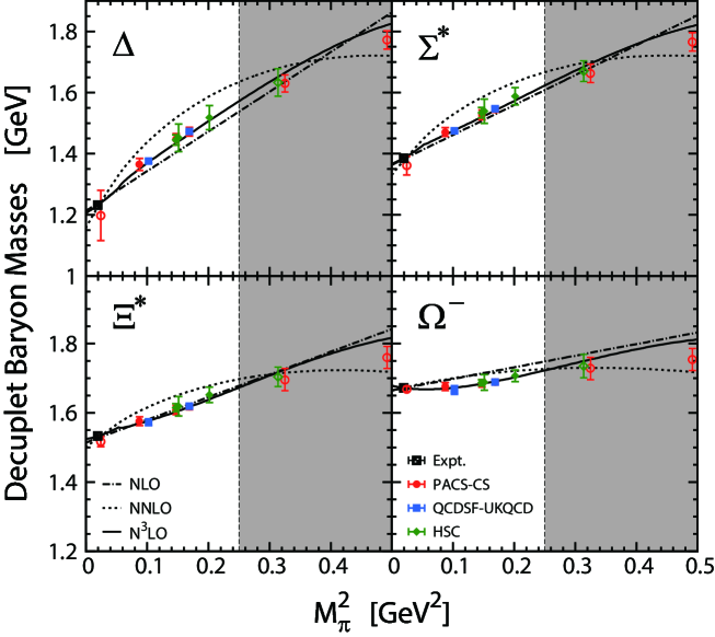
Figure 2: (Color online). Pion mass dependence of the lowest-lying decuplet baryon masses. Filled (open) symbols denote the lattice data points included in (excluded from) the fits, which are projected to have the physical strange-quark mass. The dot-dashed, the dashed, and the solid lines are the best NLO, NNLO and N³LO fits to the lattice data, respectively. In obtaining the BChPT results, the strange-quark mass has been set to its physical value. The lattice points in the shaded region are not included in the fits.

It should be emphasized that the setups of the QCDSF-UKQCD simulations are rather different from those of the PACS-CS and HSC Collaborations. Most LQCD simulations fix the strange-quark mass at (or close to ) its physical value and gradually moving the $u/d$ quark masses to their physical values. The QCDSF-UKQCD Collaboration adopted an alternative method by starting at a point on the SU(3) flavor symmetric line ($m_{u/d}=m_{s}$) and holding the sum of the quark masses $\bar{m}=(2m_{u/d}+m_{s})/3$ constant Bietenholz et al. (2010). In this way, the corresponding kaon and eta masses can be smaller than the pion mass. On the other hand, the FVCs from the kaon and eta loops can become comparable or even larger than that induced by the pion loop, because the $M_{\phi}L$ can simultaneously become smaller than $4$. Therefore, the QCDSF-UKQCD data provide us an opportunity to test the BChPT in the world of small strange-quark masses and small lattice volumes.

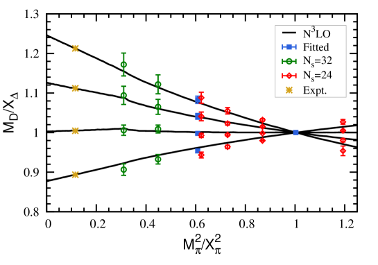
Figure 3: (Color online). The QCDSF-UKQCD lattice data Bietenholz et al. (2010) in comparison with the N³LO BChPT. The lattice data denoted by the blue filled squares are included in the fit; those by the green opened circles (with $N_{s}=32$) and the red diamonds (with $N_{s}=24$) are not. FVCs of the lattice results have been subtracted. The two-flavour singlet quantities, $X_{\pi}$ and $X_{\Delta}$, are defined as, $X_{\pi}=\sqrt{(M_{\pi}^{2}+2M_{K}^{2})/3}$, $X_{\Delta}=(2m_{\Delta}+m_{\Omega^{-}})/3$, respectively Bietenholz et al. (2010).

In Fig. 3, the QCDSF-UKQCD data are compared with the N³LO BChPT. The LQCD points included in the fit are denoted by solid points and those excluded from the fit by hollow points. All lattice points are shifted by FVCs and the kaon mass is fixed using the function $M_{K}^{2}=a+bM_{\pi}^{2}$ for the lattice ensemble with $a$ and $b$ determined in Appendix II of Ref. Ren et al. (2012). It is clear that the N³LO BChPT can describe reasonably well the QCDSF-UKQCD data obtained in both large ($N_{s}=32$) and small ($N_{s}=24$) volumes with both heavy and light pion masses. However, it should be pointed out that the ratio method eliminates to a large extent the FVCs. In other words, to plot/study the data this way one can neglect FVCs, as noticed in Ref. Bietenholz et al. (2011).

In Table 4, we show the FVCs to the LQCD data calculated in the N³LO BChPT. Most of them are at the order of a few of tens of MeV. Among them, the FVCs to the QCDSF-UKQCD data are the largest, which can be easily understood from the arguments given above.

Table 4: Finite-volume corrections (in units of MeV) to LQCD decuplet baryon masses in covariant BChPT up to N³LO.

	$M_{\pi}$	$M_{K}$	$\delta m_{\Delta}$	$\delta m_{\Sigma^{*}}$	$\delta m_{\Xi^{*}}$	$\delta m_{\Omega^{-}}$	$M_{\pi}L$	$M_{K}L$	$M_{\eta}L$
PACS-CS	296	594	14	5	0	$-3$	4.3	8.7	9.8
	384	581	5	2	1	1	5.7	8.6	9.3
	411	635	4	2	0	1	6.0	9.3	10.2
QCDSF-UKQCD	320	451	20	13	8	4	4.1	5.8	6.2
	411	411	50	50	50	50	3.95	3.95	3.95
HSC	383	544	4	2	1	0	5.7	8.1	8.8
	389	546	42	27	14	3	3.9	5.4	5.9
	449	581	28	19	11	4	4.5	5.8	6.2

We would like to point out that in the above fits we have not included the LHPC data, while in Refs. Ren et al. (2012, 2013) we have studied their data for the octet baryon masses. The reason is that the LHPC decuplet baryon data do not seem to be consistent with those of the PACS-CS, QCDSF-UKQCD, and HSC Collaborations. This is clearly demonstrated in Fig. 4, where the LHPC data are contrasted with the N³LO BChPT with the N³LO LECs tabulated in Table 3, and the corresponding kaon mass is fixed using $M_{K}^{2}=a+bM_{\pi}^{2}$ with $a$ and $b$ determined in Ref. Ren et al. (2012). It is clear that the dependencies of the lattice data on $M_{\pi}^{2}$ seem to be flatter than suggested by the N³LO BChPT. In Ref. Walker-Loud et al. (2009), it was noticed that it is difficult to extrapolate the LQCD data to the physical $\Delta(1232)$ mass. Our study seems to confirm their finding. If we had included the LHPC data(three sets of them satisfying our selection criteria) in our fitting, we would have obtained a $\chi^{2}/{\rm d.o.f.}=2.2$.

Furthermore, in order to quantify the effects of loop contributions involving virtual octet and decuplet baryons, one can allow $\mathcal{C}$ and $\mathcal{H}$ to vary in the fitting. The corresponding $\chi^{2}/{\rm d.o.f.}$ from the best fit is 0.23 with $\mathcal{C}=0.75$ and $\mathcal{H}=1.0$. It is clear that the values are consistent with the phenomenological values we used above, which can be seen as evidence for the existence of non-analytical chiral contributions following the argument given in Ref. Walker-Loud (2012). One should note, however, that because of the small difference between the $\chi^{2}/\mathrm{d.o.f.}$ obtained here and the $\chi^{2}/\mathrm{d.o.f.}$ obtained by putting $\mathcal{C}$ and $\mathcal{H}$ to zero, this evidence is rather weak in the present case.

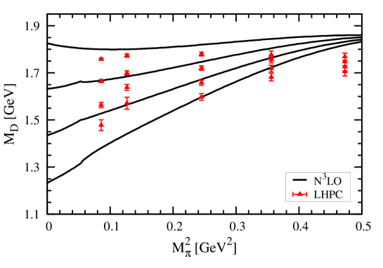
Figure 4: (Color online). Comparison between the N³LO BChPT and the LHPC data Walker-Loud et al. (2009).

III.3 Convergence of SU(3) EOMS BChPT

Convergence of BChPT in the $u$, $d$, and $s$ three-flavor sector has been under debate for many years. See, e.g., Refs.Donoghue et al. (1999); Bernard et al. (2004); Young et al. (2003); Geng (2013) and references cited therein. One prominent example is the magnetic moments of octet baryons. In Ref. Geng et al. (2008b), it has been shown that compared to the HB ChPT and the IR BChPT, the EOMS BChPT converges relatively faster. The same has been found for the octet baryon masses Martin Camalich et al. (2010). Nevertheless, even in the EOMS BChPT, convergence is relatively slow because of the large expansion parameter, $M_{K}/\Lambda_{\mathrm{ChPT}}$. Naively, each higher-order contribution is only suppressed by about one-half at the physical point, which can even be further reduced for LQCD simulations with larger light-quark masses. To speed up convergence, several alternative formulations of BChPT have been proposed, such as the long distance regularization method Donoghue et al. (1999), the cutoff scheme Bernard et al. (2004), and finite-range regulator method Young et al. (2003); Leinweber et al. (2004) BChPT, which exhibit better convergence by suppressing loop contributions with either a cutoff or a form factor.

Table 5: Contributions of different chiral orders to the decuplet baryon masses at the physical point (in units of GeV).

		$\Delta$			$\Sigma^{*}$			$\Xi^{*}$			$\Omega^{-}$
	$m_{D}$	$p^{2}$	$p^{3}$	$p^{4}$	$p^{2}$	$p^{3}$	$p^{4}$	$p^{2}$	$p^{3}$	$p^{4}$	$p^{2}$	$p^{3}$	$p^{4}$
NLO	$1.135$	$0.104$	–	–	$0.248$	–	–	$0.392$	–	–	$0.537$	–	–
NNLO	$0.870$	$0.737$	$-0.383$	–	$1.089$	$-0.582$	–	$1.441$	$-0.785$	–	$1.793$	$-0.991$	–
N3LO	$1.152$	$0.046$	$-0.429$	$0.463$	$0.158$	$-0.652$	$0.728$	$0.270$	$-0.878$	$0.988$	$0.382$	$-1.106$	$1.244$

Figure 5: Ratio of one-loop and tree contributions to the decuplet baryon masses, $\left|p^{3}/(p^{2}+m_{D})\right|$, as a function of pion mass. The strange-quark mass is set at its physical value.

Figure 6: Ratio of one-loop and tree contributions to the decuplet baryon masses, $\left|(p^{3}+p^{4})/(p^{2}+m_{D})\right|$, as a function of pion mass. The strange-quark mass is set at its physical value.

In the following, we would like to examine the contributions of different chiral orders. In Table 3 and Fig. 2, one notices that the NLO BChPT can already describe the LQCD data very well, but the experimental data are missed a little bit. Naturally one would expect that up to NNLO and N³LO, there should be some reshuffling of contributions of different orders. This can be clearly seen from Table 5, where contributions of different chiral orders to the decuplet baryon masses at the physical point are tabulated. On the other hand, once loop diagrams are included, a naive comparison of $p^{0}$ ($m_{D}$), $p^{2}$, $p^{3}$, and $p^{4}$ contributions turns out to be troubling. At NNLO, the $p^{2}$ contributions can be a factor of 2 larger than $m_{D}$, while at N³LO, the $p^{3}$ and $p^{4}$ contributions are opposite and become comparable to or even larger than the $p^{2}$ contributions, particularly for the decuplet baryons containing strangeness.

On the other hand, up to one-loop level, it might be more proper to judge convergence by comparing tree-level and loop contributions. In Figs. 5 and 6, $\left|p^{3}/(p^{2}+m_{D})\right|$ and $\left|(p^{3}+p^{4})/(p^{2}+m_{D})\right|$ are shown as a function of $M_{\pi}^{2}$. At NNLO, the $p^{3}$ contributions can reach about 50% of the tree-level contributions, while at N³LO the loop contributions become about $10\%\sim 20\%$ of the tree-level contributions. These results suggest that the chiral expansions are convergent as expected.

III.4 Pion- and strangeness-baryon sigma terms

The baryon sigma terms are important quantities in understanding the chiral condensate and the composition of the baryons. At present, there is no direct LQCD simulation of these quantities for the decuplet baryons. On the other hand, one can calculate the decuplet baryon sigma terms $\sigma_{\pi D}$ and $\sigma_{sD}$ using BChPT, once the relevant LECs are fixed, via the Feynman-Hellmann theorem by treating the decuplet baryons as stable particles as in standard BChPT. See, e.g., Ref. Ren et al. (2012) for relevant formulas.

Table 6: Pion- and strangeness-sigma terms of the decuplet baryons at the physical point. The first error is statistical and the second is systematic, estimated by taking half the difference between the N³LO result and the NNLO result.

	NNLO		N3LO
	This work	Ref. Martin Camalich et al. (2010)	This work	Ref. Semke and Lutz (2012b)
$\sigma_{\pi\Delta}$ [MeV]	$64(1)$	$55(4)(18)$	$28(1)(18)$	$34(3)$
$\sigma_{\pi\Sigma^{*}}$ [MeV]	$44(1)$	$39(3)(13)$	$22(2)(11)$	$28(2)$
$\sigma_{\pi\Xi^{*}}$ [MeV]	$26(1)$	$22(3)(7)$	$11(2)(8)$	$18(4)$
$\sigma_{\pi\Omega^{-}}$ [MeV]	$8(1)$	$5(2)(1)$	$-5(2)(6)$	$10(4)$
$\sigma_{s\Delta}$ [MeV]	$93(12)$	$56(24)(1)$	$88(22)(3)$	$41(41)$
$\sigma_{s\Sigma^{*}}$ [MeV]	$181(13)$	$160(28)(7)$	$243(24)(31)$	$211(44)$
$\sigma_{s\Xi^{*}}$ [MeV]	$258(14)$	$274(32)(9)$	$391(24)(67)$	$373(53)$
$\sigma_{s\Omega^{-}}$ [MeV]	$326(15)$	$360(34)(26)$	$528(26)(101)$	$510(50)$

Using the LECs given in Table 3, we calculate the sigma terms of the baryon decuplet at the physical point, and the results are listed in Table 6. For comparison, we also tabulate the results of Refs. Martin Camalich et al. (2010); Semke and Lutz (2012b). The difference between our $\mathcal{O}(p^{3})$ predictions with those of Ref. Martin Camalich et al. (2010) reflects the influence of the LQCD data and the fitting strategy. While our N³LO results are consistent with those of Ref. Semke and Lutz (2012b) within uncertainties.

IV Summary

We have studied the ground-state decuplet baryon masses in baryon chiral perturbation theory with the extended-on-mass-shell scheme up to next-to-next-to-next-to-leading order. Through a simultaneous fit of the $n_{f}=2+1$ LQCD data from the PACS-CS, QCDSF-UKQCD, and HSC Collaborations, the $14$ unknown low-energy constants are determined. In fitting the LQCD data, finite-volume corrections are taken into account self-consistently. A $\chi^{2}/{\rm d.o.f.}=0.20$ is achieved for the eight sets of LQCD data satisfying $M_{\pi}^{2}<0.25$ GeV² and $M_{\phi}L>3.8$.

Our studies show that the chiral expansions are convergent as expected and the results of the PACS-CS, QCDSF-UKQCD, and HSC Collaborations seem to be consistent with each other, but not those of the LHPC Collaboration. We have calculated the sigma terms of the decuplet baryons by use of the Feynman-Hellmann theorem, which should be compared to future LQCD data.

It should be noted that our present study suffers from the limited range of the LQCD data (in terms of the input parameters) and the rather large number of unknown low-energy constants. Future refined LQCD simulations with various light-quark and strange-quark masses, lattice volume and lattice spacing will be extremely welcome to put covariant baryon chiral perturbation theory to a more stringent test than was done in the present work. In the context of effective field theories, one would like to apply the same formalism and utilize the same low-energy constants to study other related physical observables, which can also serve as an additional test. Such works are in progress and will be reported elsewhere.

V Appendix

Here we show explicitly the N³LO loop functions appearing in Eq. (13), which are calculated in the EOMS scheme:

$$H_{D}^{(e,1)}(M_{\phi}) = M_{\phi}^{2}\left[1+{\rm ln}\left(\frac{\mu^{2}}{M_{\phi}^{2}}\right)\right],$$ (31)

$$H_{D}^{(e,2)}(M_{\phi}) = M_{\phi}^{4}\left[1+{\rm ln}\left(\frac{\mu^{2}}{M_{\phi}^{2}}\right)\right],$$ (32)

$$H_{D}^{(e,3)}(M_{\phi}) = m_{D}\left\{\frac{M_{\phi}^{4}}{4}\left[1+{\rm ln}\left(\frac{\mu^{2}}{M_{\phi}^{2}}\right)\right]+\frac{1}{8}M_{\phi}^{4}\right\}.$$ (33)

$$H_{D,B}^{(f)}(M_{\phi}) = \frac{1}{144m_{D}^{4}}m_{D}^{(2)}M_{\phi}^{2}\left[90m_{0}^{4}+96m_{0}^{3}m_{D}+36m_{0}^{2}m_{D}^{2}+48m_{0}m_{D}^{3}-22m_{D}^{4}\right.$$ (34)

$$\quad\left.-3\left(30m_{0}^{2}+16m_{0}m_{D}+19m_{D}^{2}\right)M_{\phi}^{2}+30M_{\phi}^{4}\right]$$

$$-\frac{1}{12m_{D}^{3}}m_{B}^{(2)}M_{\phi}^{2}\left[8m_{0}^{3}+8m_{0}^{2}m_{D}+4m_{0}m_{D}^{2}+7m_{D}^{3}-(4m_{0}+m_{D})M_{\phi}^{2}\right]$$

$$+\frac{1}{24m_{D}^{6}}m_{D}^{(2)}M_{\phi}^{2}\ln\left(\frac{M_{\phi}}{m_{0}}\right)\left[4m_{0}^{5}(5m_{0}+6m_{D})\right.$$

$$\left.\quad-6(5m_{0}^{4}+4m_{0}^{3}m_{D}+3m_{0}^{2}m_{D}^{2}+2m_{0}m_{D}^{3}+m_{D}^{4})M_{\phi}^{2}+4(5m_{0}^{2}+2m_{0}m_{D}+3m_{D}^{2})M_{\phi}^{4}-5M_{\phi}^{6}\right]$$

$$-\frac{1}{12m_{D}^{5}}m_{B}^{(2)}M_{\phi}^{2}\ln\left(\frac{M_{\phi}}{m_{0}}\right)\left[3m_{0}^{4}(4m_{0}+5m_{D})\right.$$

$$\left.\quad-3(4m_{0}^{3}+3m_{0}^{2}m_{D}+2m_{0}m_{D}^{2}+m_{D}^{3})M_{\phi}^{2}+(4m_{0}+m_{D})M_{\phi}^{4}\right]$$

$$+\frac{1}{24m_{D}^{6}}(m_{0}-m_{D})^{2}(m_{0}+m_{D})^{4}\left[\ln(m_{0}M_{\phi})-\ln(m_{0}^{2}-m_{D}^{2})-i\pi\right]$$

$$\quad\times\left[2m_{D}m_{B}^{(2)}(4m_{0}-m_{D})-m_{D}^{(2)}(5m_{0}^{2}-2m_{0}m_{D}+3m_{D}^{2})\right]$$

$$+\frac{1}{12}M_{\phi}^{2}\left(3m_{B}^{(2)}+2m_{D}^{(2)}\right)\ln\left(\frac{m_{0}M_{\phi}}{\mu^{2}}\right)$$

$$+\frac{1}{24m_{D}^{6}\sqrt{\mathcal{W}}}(m_{0}^{2}-2m_{0}m_{D}+m_{D}^{2}-M_{\phi}^{2})(m_{0}^{2}+2m_{0}m_{D}+m_{D}^{2}-M_{\phi}^{2})^{2}$$

$$\quad\times\left[5m_{0}^{4}m_{D}^{(2)}-2m_{0}^{2}\left(5M_{\phi}^{2}m_{D}^{(2)}+m_{D}^{2}\left(m_{D}^{(2)}-m_{B}^{(2)}\right)\right)-2m_{0}^{3}m_{D}\left(m_{D}^{(2)}+4m_{B}^{(2)}\right)\right.$$

$$\quad\quad\left.+2m_{0}m_{D}(m_{D}^{2}+M_{\phi}^{2})\left(m_{D}^{(2)}+4m_{B}^{(2)}\right)-(m_{D}^{2}-M_{\phi}^{2})\left(5M_{\phi}^{2}m_{D}^{(2)}+m_{D}^{2}\left(3m_{D}^{(2)}+2m_{B}^{(2)}\right)\right)\right]$$

$$\quad\times\left[\arctan\left(\frac{m_{0}^{2}-m_{D}^{2}-M_{\phi}^{2}}{\sqrt{\mathcal{W}}}\right)-\arctan\left(\frac{m_{0}^{2}+m_{D}^{2}-M_{\phi}^{2}}{\sqrt{\mathcal{W}}}\right)\right],$$

$$H_{D,D^{\prime}}^{(g)}(M_{\phi}) = \frac{M_{\phi}^{2}}{432m_{D}^{4}}\left[4m_{D}^{4}\left(132m_{D}^{(2)}-97m_{D^{\prime}}^{(2)}\right)\right.$$ (35)

$$\quad\left.+30M_{\phi}^{4}\left(3m_{D}^{(2)}+2m_{D^{\prime}}^{(2)}\right)-15m_{D}^{2}M_{\phi}^{2}\left(31m_{D}^{(2)}+14m_{D^{\prime}}^{(2)}\right)\right]$$

$$+\frac{5M_{\phi}^{2}}{72m_{D}^{6}}\ln\left(\frac{M_{\phi}}{m_{D}}\right)\left[-30m_{D}^{4}M_{\phi}^{2}m_{D}^{(2)}+48m_{D}^{6}\left(m_{D}^{(2)}-m_{D^{\prime}}^{(2)}\right)\right.$$

$$\quad\left.+10m_{D}^{2}M_{\phi}^{4}\left(2m_{D}^{(2)}+m_{D^{\prime}}^{(2)}\right)-M_{\phi}^{6}\left(3m_{D}^{(2)}+2m_{D^{\prime}}^{(2)}\right)\right]$$

$$+\frac{5M_{\phi}^{2}}{36}\left(12m_{D}^{(2)}-7m_{D^{\prime}}^{(2)}\right)\ln\left(\frac{m_{D}^{2}}{\mu^{2}}\right)$$

$$-\frac{5}{72m_{D}^{6}}M_{\phi}^{3}(4m_{D}^{2}-M_{\phi}^{2})^{3/2}\left[2m_{D}^{2}\left(m_{D}^{(2)}-m_{D^{\prime}}^{(2)}\right)-M_{\phi}^{2}\left(3m_{D}^{(2)}+2m_{D^{\prime}}^{(2)}\right)\right]$$

$$\quad\times\left[\arctan\left(\frac{M_{\phi}}{\sqrt{4m_{D}^{2}-M_{\phi}^{2}}}\right)+\arctan\left(\frac{2m_{D}^{2}-M_{\phi}^{2}}{M_{\phi}\sqrt{4m_{D}^{2}-M_{\phi}^{2}}}\right)\right].$$

In Eqs. (34) and (35), $\mathcal{W}=-m_{0}^{4}-(m_{D}^{2}-M_{\phi}^{2})^{2}+2m_{0}^{2}(m_{D}^{2}+M_{\phi}^{2})$, $m_{D}^{(2)}$ and $m_{B}^{(2)}$ are the NLO decuplet and octet baryon masses, where $m_{D}^{(2)}$ is given in Eq. (13), and $m_{B}^{(2)}$ has the following form:

$$m_{B}^{(2)}=\sum\limits_{\phi=\pi,~{}K}\xi_{B,\phi}^{(2)}M_{\phi}^{2}$$ (36)

with the corresponding coefficients $\xi_{B,\phi}^{(2)}$ listed in Table 7.

Table 7: Coefficients of the NLO contributions to the octet baryon masses [Eq. (36)].

	$N$	$\Lambda$	$\Sigma$	$\Xi$
$\xi^{(a)}_{B,\pi}$	$-(2b_{0}+4b_{F})$	$\frac{-2}{3}(3b_{0}-2b_{D})$	$-(2b_{0}+4b_{D})$	$-(2b_{0}-4b_{F})$
$\xi^{(a)}_{B,K}$	$-(4b_{0}+4b_{D}-4b_{F})$	$\frac{-2}{3}(6b_{0}+8b_{D})$	$-4b_{0}$	$-(4b_{0}+4b_{D}+4b_{F})$

References

- Durr et al. (2008) S. Durr, Z. Fodor, J. Frison, C. Hoelbling, R. Hoffmann, et al., Science 322, 1224 (2008), arXiv:0906.3599 [hep-lat] .
- Alexandrou et al. (2009) C. Alexandrou et al. (ETM Collaboration), Phys.Rev. D80, 114503 (2009), arXiv:0910.2419 [hep-lat] .
- Aoki et al. (2009) S. Aoki et al. (PACS-CS Collaboration), Phys.Rev. D79, 034503 (2009), arXiv:0807.1661 [hep-lat] .
- Aoki et al. (2010) S. Aoki et al. (PACS-CS Collaboration), Phys.Rev. D81, 074503 (2010), arXiv:0911.2561 [hep-lat] .
- Walker-Loud et al. (2009) A. Walker-Loud, H.-W. Lin, D. Richards, R. Edwards, M. Engelhardt, et al., Phys.Rev. D79, 054502 (2009), arXiv:0806.4549 [hep-lat] .
- Lin et al. (2009) H.-W. Lin et al. (Hadron Spectrum Collaboration), Phys.Rev. D79, 034502 (2009), arXiv:0810.3588 [hep-lat] .
- Bietenholz et al. (2010) W. Bietenholz, V. Bornyakov, N. Cundy, M. Gockeler, R. Horsley, et al., Phys.Lett. B690, 436 (2010), arXiv:1003.1114 [hep-lat] .
- Bietenholz et al. (2011) W. Bietenholz, V. Bornyakov, M. Gockeler, R. Horsley, W. Lockhart, et al., Phys.Rev. D84, 054509 (2011), arXiv:1102.5300 [hep-lat] .
- Beane et al. (2011) S. Beane, E. Chang, W. Detmold, H. Lin, T. Luu, et al., Phys.Rev. D84, 014507 (2011), arXiv:1104.4101 [hep-lat] .
- Fodor and Hoelbling (2012) Z. Fodor and C. Hoelbling, Rev.Mod.Phys. 84, 449 (2012), arXiv:1203.4789 [hep-lat] .
- Beringer et al. (2012) J. Beringer et al. (Particle Data Group), Phys.Rev. D86, 010001 (2012).
- Durr et al. (2011) S. Durr, Z. Fodor, C. Hoelbling, S. Katz, S. Krieg, et al., JHEP 1108, 148 (2011), arXiv:1011.2711 [hep-lat] .
- Bazavov et al. (2013a) A. Bazavov et al. (MILC Collaboration), Phys.Rev. D87, 054505 (2013a), arXiv:1212.4768 [hep-lat] .
- Bazavov et al. (2013b) A. Bazavov et al. (MILC Collaboration), Phys.Rev.Lett. 110, 172003 (2013b), arXiv:1301.5855 [hep-ph] .
- Weinberg (1979) S. Weinberg, Physica A96, 327 (1979).
- Gasser and Leutwyler (1984) J. Gasser and H. Leutwyler, Annals Phys. 158, 142 (1984).
- Gasser and Leutwyler (1985) J. Gasser and H. Leutwyler, Nucl.Phys. B250, 465 (1985).
- Gasser et al. (1988) J. Gasser, M. Sainio, and A. Svarc, Nucl.Phys. B307, 779 (1988).
- Leutwyler (1994) H. Leutwyler, (1994), arXiv:hep-ph/9406283 [hep-ph] .
- Bernard et al. (1995) V. Bernard, N. Kaiser, and U.-G. Meissner, Int.J.Mod.Phys. E4, 193 (1995), arXiv:hep-ph/9501384 [hep-ph] .
- Pich (1995) A. Pich, Rept.Prog.Phys. 58, 563 (1995), arXiv:hep-ph/9502366 [hep-ph] .
- Ecker (1995) G. Ecker, Prog.Part.Nucl.Phys. 35, 1 (1995), arXiv:hep-ph/9501357 [hep-ph] .
- Pich (1998) A. Pich, (1998), arXiv:hep-ph/9806303 [hep-ph] .
- Bernard and Meissner (2007) V. Bernard and U.-G. Meissner, Ann.Rev.Nucl.Part.Sci. 57, 33 (2007), arXiv:hep-ph/0611231 [hep-ph] .
- Bernard (2008) V. Bernard, Prog.Part.Nucl.Phys. 60, 82 (2008), arXiv:0706.0312 [hep-ph] .
- Scherer and Schindler (2012) S. Scherer and M. R. Schindler, Lect.Notes Phys. 830, 1 (2012).
- Leinweber et al. (2004) D. B. Leinweber, A. W. Thomas, and R. D. Young, Phys.Rev.Lett. 92, 242002 (2004), arXiv:hep-lat/0302020 [hep-lat] .
- Bernard et al. (2004) V. Bernard, T. R. Hemmert, and U.-G. Meissner, Nucl.Phys. A732, 149 (2004), arXiv:hep-ph/0307115 [hep-ph] .
- Procura et al. (2004) M. Procura, T. R. Hemmert, and W. Weise, Phys.Rev. D69, 034505 (2004), arXiv:hep-lat/0309020 [hep-lat] .
- Bernard et al. (2005) V. Bernard, T. R. Hemmert, and U.-G. Meissner, Phys.Lett. B622, 141 (2005), arXiv:hep-lat/0503022 [hep-lat] .
- Ali Khan et al. (2004) A. Ali Khan et al. (QCDSF-UKQCD Collaboration), Nucl.Phys. B689, 175 (2004), arXiv:hep-lat/0312030 [hep-lat] .
- Beane (2004) S. R. Beane, Phys.Rev. D70, 034507 (2004), arXiv:hep-lat/0403015 [hep-lat] .
- Beane and Savage (2003) S. R. Beane and M. J. Savage, Phys.Rev. D68, 114502 (2003), arXiv:hep-lat/0306036 [hep-lat] .
- Arndt and Tiburzi (2004) D. Arndt and B. C. Tiburzi, Phys.Rev. D69, 114503 (2004), arXiv:hep-lat/0402029 [hep-lat] .
- Jenkins and Manohar (1991) E. E. Jenkins and A. V. Manohar, Phys.Lett. B255, 558 (1991).
- Becher and Leutwyler (1999) T. Becher and H. Leutwyler, Eur.Phys.J. C9, 643 (1999), arXiv:hep-ph/9901384 [hep-ph] .
- Gegelia and Japaridze (1999) J. Gegelia and G. Japaridze, Phys.Rev. D60, 114038 (1999), arXiv:hep-ph/9908377 [hep-ph] .
- Fuchs et al. (2003) T. Fuchs, J. Gegelia, G. Japaridze, and S. Scherer, Phys.Rev. D68, 056005 (2003), arXiv:hep-ph/0302117 [hep-ph] .
- Jenkins (1992) E. E. Jenkins, Nucl.Phys. B368, 190 (1992).
- Bernard et al. (1993) V. Bernard, N. Kaiser, and U. G. Meissner, Z.Phys. C60, 111 (1993), arXiv:hep-ph/9303311 [hep-ph] .
- Banerjee and Milana (1995) M. Banerjee and J. Milana, Phys.Rev. D52, 6451 (1995), arXiv:hep-ph/9410398 [hep-ph] .
- Borasoy and Meissner (1997) B. Borasoy and U.-G. Meissner, Annals Phys. 254, 192 (1997), arXiv:hep-ph/9607432 [hep-ph] .
- Walker-Loud (2005) A. Walker-Loud, Nucl.Phys. A747, 476 (2005), arXiv:hep-lat/0405007 [hep-lat] .
- Ellis and Torikoshi (2000) P. Ellis and K. Torikoshi, Phys.Rev. C61, 015205 (2000), arXiv:nucl-th/9904017 [nucl-th] .
- Frink and Meissner (2004) M. Frink and U.-G. Meissner, JHEP 0407, 028 (2004), arXiv:hep-lat/0404018 [hep-lat] .
- Frink et al. (2005) M. Frink, U.-G. Meissner, and I. Scheller, Eur.Phys.J. A24, 395 (2005), arXiv:hep-lat/0501024 [hep-lat] .
- Lehnhart et al. (2005) B. Lehnhart, J. Gegelia, and S. Scherer, J.Phys. G31, 89 (2005), arXiv:hep-ph/0412092 [hep-ph] .
- Semke and Lutz (2006) A. Semke and M. Lutz, Nucl.Phys. A778, 153 (2006), arXiv:nucl-th/0511061 [nucl-th] .
- Semke and Lutz (2007) A. Semke and M. Lutz, Nucl.Phys. A789, 251 (2007).
- Martin Camalich et al. (2010) J. Martin Camalich, L. S. Geng, and M. Vicente Vacas, Phys.Rev. D82, 074504 (2010), arXiv:1003.1929 [hep-lat] .
- Geng et al. (2011) L. S. Geng, X.-L. Ren, J. Martin-Camalich, and W. Weise, Phys.Rev. D84, 074024 (2011), arXiv:1108.2231 [hep-ph] .
- Young and Thomas (2010) R. Young and A. Thomas, Phys.Rev. D81, 014503 (2010), arXiv:0901.3310 [hep-lat] .
- Semke and Lutz (2012a) A. Semke and M. Lutz, Phys.Rev. D85, 034001 (2012a), arXiv:1111.0238 [hep-ph] .
- Semke and Lutz (2012b) A. Semke and M. Lutz, Phys.Lett. B717, 242 (2012b), arXiv:1202.3556 [hep-ph] .
- Lutz and Semke (2012) M. Lutz and A. Semke, Phys.Rev. D86, 091502 (2012), arXiv:1209.2791 [hep-lat] .
- Bruns et al. (2013) P. C. Bruns, L. Greil, and A. Schafer, Phys.Rev. D87, 054021 (2013), arXiv:1209.0980 [hep-ph] .
- Ren et al. (2012) X.-L. Ren, L. Geng, J. Martin Camalich, J. Meng, and H. Toki, J. High Energy Phys. 12, 073 (2012), arXiv:1209.3641 [nucl-th] .
- Ren et al. (2013) X.-L. Ren, L. Geng, J. Meng, and H. Toki, Phys.Rev. D87, 074001 (2013), arXiv:1302.1953 [nucl-th] .
- Ishikawa et al. (2009) K.-I. Ishikawa et al. (PACS-CS Collaboration), Phys.Rev. D80, 054502 (2009), arXiv:0905.0962 [hep-lat] .
- Pascalutsa (1998) V. Pascalutsa, Phys.Rev. D58, 096002 (1998), arXiv:hep-ph/9802288 [hep-ph] .
- Pascalutsa and Timmermans (1999) V. Pascalutsa and R. Timmermans, Phys.Rev. C60, 042201 (1999), arXiv:nucl-th/9905065 [nucl-th] .
- Geng et al. (2008a) L. S. Geng, J. Martin Camalich, L. Alvarez-Ruso, and M. Vicente Vacas, Phys.Rev. D78, 014011 (2008a), arXiv:0801.4495 [hep-ph] .
- Lutz and Semke (2011) M. Lutz and A. Semke, Phys.Rev. D83, 034008 (2011), arXiv:1012.4365 [hep-ph] .
- Tiburzi and Walker-Loud (2005) B. C. Tiburzi and A. Walker-Loud, Nucl.Phys. A748, 513 (2005), arXiv:hep-lat/0407030 [hep-lat] .
- Pascalutsa and Vanderhaeghen (2006) V. Pascalutsa and M. Vanderhaeghen, Phys.Lett. B636, 31 (2006), arXiv:hep-ph/0511261 [hep-ph] .
- Geng (2013) L. S. Geng, Front.Phys.China. 8, 328 (2013), arXiv:1301.6815 [nucl-th] .
- Bijnens and Jemos (2012) J. Bijnens and I. Jemos, Nucl.Phys. B854, 631 (2012), arXiv:1103.5945 [hep-ph] .
- Bernard et al. (2008) V. Bernard, U.-G. Meissner, and A. Rusetsky, Nucl.Phys. B788, 1 (2008), arXiv:hep-lat/0702012 [HEP-LAT] .
- Ren et al. (2014) X.-L. Ren, L.-S. Geng, and J. Meng, Eur.Phys.J. C74, 2754 (2014), arXiv:1311.7234 [hep-ph] .
- Alarcon et al. (2014) J. Alarcon, L. Geng, J. Martin Camalich, and J. Oller, Phys.Lett. B730, 342 (2014), arXiv:1209.2870 [hep-ph] .
- Walker-Loud (2012) A. Walker-Loud, Phys.Rev. D86, 074509 (2012), arXiv:1112.2658 [hep-lat] .
- Donoghue et al. (1999) J. F. Donoghue, B. R. Holstein, and B. Borasoy, Phys.Rev. D59, 036002 (1999), arXiv:hep-ph/9804281 [hep-ph] .
- Young et al. (2003) R. D. Young, D. B. Leinweber, and A. W. Thomas, Prog.Part.Nucl.Phys. 50, 399 (2003), arXiv:hep-lat/0212031 [hep-lat] .
- Descotes-Genon et al. (2004) S. Descotes-Genon, N. Fuchs, L. Girlanda, and J. Stern, Eur.Phys.J. C34, 201 (2004), arXiv:hep-ph/0311120 [hep-ph] .
- Bernard et al. (2011) V. Bernard, S. Descotes-Genon, and G. Toucas, JHEP 1101, 107 (2011), arXiv:1009.5066 [hep-ph] .
- Geng et al. (2008b) L. S. Geng, J. Martin Camalich, L. Alvarez-Ruso, and M. Vicente Vacas, Phys.Rev.Lett. 101, 222002 (2008b), arXiv:0805.1419 [hep-ph] .