New evolutionary sequences for extremely low mass white dwarfs:

Abstract

Context. The number of detected extremely low mass (ELM) white dwarf stars has increased drastically in recent year thanks to the results of many surveys. In addition, some of these stars have been found to exhibit pulsations, making them potential targets for asteroseismology.

Aims. We provide a fine and homogeneous grid of evolutionary sequences for helium (He) core white dwarfs for the whole range of their expected masses ($0.15\lesssim M_{*}/M_{\sun}\lesssim 0.45$), including the mass range for ELM white dwarfs ($M_{*}/M_{\sun}\lesssim 0.20$). The grid is appropriate for mass and age determination of these stars, as well as to study their adiatabic pulsational properties.

Methods. White dwarf sequences have been computed by performing full evolutionary calculations that consider the main energy sources and processes of chemical abundance changes during white dwarf evolution. Realistic initial models for the evolving white dwarfs have been obtained by computing the non-conservative evolution of a binary system consisting of an initially $1M_{\odot}$ ZAMS star and a $1.4M_{\odot}$ neutron star for various initial orbital periods. To derive cooling ages and masses for He-core white dwarf we perform a least square fitting of the $M(T_{\rm eff},g)$ and ${\rm Age}(T_{\rm eff},g)$ relations provided by our sequences by using a scheme that takes into account the time spent by models in different regions of the $T_{\rm eff}-g$ plane. This is particularly useful when multiple solutions for cooling age and mass determinations are possible in the case of CNO-flashing sequences. We also explore in a preliminary way the adiabatic pulsational properties of models near the critical mass for the development of CNO flashes ($\sim 0.2M_{\odot}$). This is motivated by the discovery of pulsating white dwarfs with stellar masses near this threshold value.

Results. We obtain reliable and homogeneous mass and cooling age determinations for 58 very low-mass white dwarfs, including 3 pulsating stars. Also, we find substantial differences in the period spacing distributions of $g$-modes for models with stellar masses near $\sim 0.2M_{\odot}$, which could be used as a seismic tool to distinguish stars that have undergone CNO flashes in their early cooling phase from those that have not. Finally, for an easy application of our results, we provide a reduced grid of values useful to obtain masses and ages of He-core white dwarf.

1 Introduction

White dwarf stars are routinely used to constrain the age and past history of the Galactic populations, including the solar neighborhood, open and globular clusters (Von Hippel & Gilmore 2000; Hansen et al. 2007; Winget et al. 2009; García-Berro et al. 2010; Bono et al. 2013, and references therein). In addition, they are used to place constraints on properties of elementary particles such as axions (Isern et al. 1992; Isern et al. 2008; Córsico et al. 2012a,b), and neutrinos (Winget et al. 2004) or on alternative theories of gravitation (García–Berro et al. 1995; García–Berro et al. 2011). These and other potential applications of white dwarfs require a detailed and precise knowledge of the main physical processes that control their evolution (see Fontaine & Brassard 2008; Winget & Kepler 2008 and Althaus et al. 2010a for a review).

The white dwarf mass distribution includes a population of low-mass remnants, most of them expected to have a helium (He) core in their interiors (see Kepler et al. 2007). In recent years, the number of detected white dwarfs with very low stellar masses, commonly referred to as Extremely Low Mass (ELM) white dwarfs, has increased considerably thanks to the result of many surveys, in particular the ELM survey, and the SPY and WASP surveys (see Koester et al. 2009; Brown et al. 2010; Maxted et al. 2011, Brown et al. 2012). Because of the very low stellar mass values that characterize these ELM white dwarfs (lower than about 0.20 $M_{\sun}$), they are believed to be the result of compact binary evolution, during which the envelope of a red giant star is removed before the core reaches enough mass to ignite helium. The evolution of He-core white dwarfs has been studied by Driebe et al. (1998), Sarna et al. (2000), Althaus et al. (2001), Serenelli et al. (2002), Nelson et al. (2004), Benvenuto & De Vito (2005), Panei et al. (2007), and more recently by Gautschy (2013).

A major step towards the understanding of the formation and evolution of ELM white dwarfs has been the recent discovery of three pulsating He-core white dwarfs with stellar masses below 0.23 $M_{\sun}$ and effective temperatures less than 10,000K (Hermes et al. 2012, 2013). This new class of pulsating white dwarfs most probably belongs to a low-mass extention of the ZZ Ceti instability strip to much cooler effective temperatures. It is expected that the application of the tools of asteroseismology to these and other pulsating ELM white dwarfs being found in the future will reveal details of their internal structure and evolutionary status; see Steinfadt (2010) and Córsico et al. (2012) for the first exploration of the adiabatic properties of these objects.

The development of a fine and homogeneous grid of evolutionary sequences for He-core white dwarfs, and in particular ELM white dwarfs, derived consistently from binary evolution is therefore a pressing necessity for precise mass and cooling age determinations, and asteroseismological inferences for these stars. This is precisely the main aim of this paper. As shown by Sarna et al. (2000) a proper treatment of the binary evolution leading to the formation of these stars is of utmost importance for the correct assessment of their evolutionay properties. This is particularly true regarding the mass of the hydrogen envelope that is left after the end of binary evolution. In particular, Sarna et al. (2000) found that for stellar masses lower than $\approx 0.25M_{\sun}$, binary evolution calculations yield more massive hydrogen envelopes than those found by arbitrarily abstracting mass to a red giant star. These authors also reported that during the evolution through the stages at approximately constant luminosity that follow the end of binary evolution, and also during most of the cooling branch, an active hydrogen burning shell remains, delaying the evolution of ELM white dwarfs by several Gyr. In this connection, Sarna et al. (2000) found that the evolutionary times during the stages of constant luminosity are strongly dependent on the mass of the white dwarf remnant. Hence, for a proper assessment of evolutionary timescales and mass-radius relations, the binary nature that leads to the formation of ELM white dwarfs must be taken into account. This has been the approach we adopted in this work to generate the initial models for the evolving white dwarfs. Specifically, we have considered the non-conservative angular-momentum evolution of a binary system consisting of an initially $1M_{\odot}$ ZAMS component and a $1.4M_{\odot}$ neutron star as the other component. In particular, our white dwarf sequences start shortly after the end of Roche lobe phase.

In addition to the discussion of the evolutionary expectations of our sequences, we extend the scope of the paper by presenting a preliminary exploration of the adiabatic pulsational properties of our evolutionary models near the critical stellar mass for the development of CNO flashes on the cooling branch. We show in particular that seismic tools exploiting these properties can be used to extract information about the occurrence of CNO flashes in prior stages, and the consequent age dichotomy expected in low-mass He-core white dwarfs. Our interest in this aspect is motivated by the fact that the three pulsating ELM white dwarfs discovered by Hermes et al. (2013) have stellar mass precisely near the threshold value for the occurrence of CNO flashes.

The paper is outlined as follows. In Sect. 2 we briefly describe the input physics of the evolutionary code employed in our calculations, and the procedure and assumptions we consider for the computation of binary evolution that leads to the formation of ELM white dwarfs. In total, 9 initial ELM white dwarf models with stellar masses between 0.155 and 0.20 $\,M_{\sun}$ have been derived for initial orbital periods at the beginning of the Roche lobe phase in the range 0.9 to 2 d. Additional binary calculations have been conducted for binary configurations with initial orbital periods up to 300d to cover the whole mass range expected for He-core white dwarfs. In Sect. 3 the main evolutionary characteristics of our sequences are presented, while in Sect. 4 we describe the method adopted to derive from these sequences ages and masses for He-core white dwarfs. In this Section we also present a new and homogeneous determination of masses and, for the first time, cooling ages of a large sample of recently discovered low-mass (most of them ELM) white dwarfs, and a simple algorithm for an easy use of our sequences as well. In Sect. 5 we describe the main basic expectations of our sequences for the adiabatic pulsation properties of models representative of the observed pulsating ELM white dwarfs.

Table 1: Characteristics of our initial He-core white dwarf models.

$M_{\rm f}(M_{\sun})$	$P_{\rm i}$(d)	$P_{\rm f}$(d)	$X_{\rm f}^{\rm surf}$	$M_{\rm H}$	H flash
0.15540	0.90	0.23	0.365	$4.34\times 10^{-3}$	No
0.16115	0.95	0.32	0.376	$4.19\times 10^{-3}$	No
0.16499	1.0	0.35	0.390	$4.09\times 10^{-3}$	No
0.17064	1.1	0.44	0.405	$3.94\times 10^{-3}$	No
0.17624	1.2	0.54	0.423	$3.80\times 10^{-3}$	No
0.18213	1.3	0.80	0.440	$3.66\times 10^{-3}$	Yes
(0.18050)
0.18685	1.4	1.14	0.453	$3.55\times 10^{-3}$	Yes
(0.18630)
0.19210	1.55	1.54	0.466	$3.42\times 10^{-3}$	Yes
(0.19173)
0.20258	2	2.47	0.490	$3.22\times 10^{-3}$	Yes
(0.20187)
0.23903	5.2	10.32	0.701	$2.86\times 10^{-3}$	Yes
(0.23887)
0.27242	10	20.4	0.715	$2.02\times 10^{-3}$	Yes
(0.27065)
0.32079	40	78.7	0.715	$1.18\times 10^{-3}$	Yes
(0.32048)
0.36304	100	187.7	0.715	$7.85\times 10^{-4}$	Yes
(0.36242)
0.43520	300	520	0.715	$4.33\times 10^{-4}$	No

2 Numerical tools

The evolutionary calculations presented in this work have been done using the LPCODE stellar evolutionary code (Althaus et al. 2003, 2005, 2012). This code has recently been used to produce very accurate white dwarf models – see García–Berro et al. (2010), Althaus et al. (2010b), Renedo et al. (2010), Miller Bertolami et al. (2011ab), and references therein. The code has also been used to study the formation of subdwarf stars from the post-red giant branch hot-flasher scenario (Miller Bertolami et al. 2008), and the role of thermohaline mixing for the surface composition of low-mass giant stars (Wachlin et al. 2011). A complete description of the input physics and numerical procedures can be found in these works. The nuclear network accounts explicitly for the following elements: ¹H, ²H, ³He, ⁴He, ⁷Li, ⁷Be, ¹²C, ¹³C, ¹⁴N, ¹⁵N, ¹⁶O, ¹⁷O, ¹⁸O, ¹⁹F, ²⁰Ne and ²²Ne, together with 34 thermonuclear reaction rates for the pp-chains, CNO bi-cycle, helium burning, and C ignition that are identical to those described in Althaus et al. (2005), with the exception of ¹²C$\ +\$p$\rightarrow\ ^{13}$N + $\gamma\rightarrow\ ^{13}$C + e${}^{+}+\nu_{\rm e}$ and ¹³C(p,$\gamma)^{14}$N, which are taken from Angulo et al. (1999). Radiative opacities are those of OPAL (Iglesias & Rogers 1996). Conductive opacities are from Cassisi et al. (2007). The equation of state during the main sequence evolution is that of OPAL for hydrogen- and helium-rich composition, and a given metallicity. Finally, updated low-temperature molecular opacities with varying C/O ratios are used. To this end, we have adopted the low temperature opacities computed at Wichita State University (Ferguson et al. 2005) and presented by Weiss & Ferguson (2009). In LPCODE molecular opacities are computed by adopting the opacity tables with the correct abundances of the unenhanced metals (e.g. Fe) and C/O ratio. Interpolation is carried out by means of separate cuadratic interpolations in $R=\rho/{T_{6}}^{3}$, $T$ and $X_{\rm H}$, but linearly in $N_{\rm C}/N_{\rm O}$.

For the evolutionary stages following the end of mass loss, and for the white dwarf regime, we use the equation of state of Magni & Mazzitelli (1979) for the whole star. We also take into account the effects of element diffusion due to gravitational settling, chemical and thermal diffusion of ¹H, ³He, ⁴He, ¹²C, ¹³C, ¹⁴N and ¹⁶O, see Althaus et al. (2003) for details. In particular, the metal mass fraction $Z$ in the envelope of our models is specified by scaling it to the local abundance of the CNO elements at each layer. For the white dwarf regime and for effective temperatures lower than 10,000 K, outer boundary conditions for the evolving models are derived from non-grey model atmospheres (Rohrmann et al. 2012). Recently, LPCODE has been tested against other white dwarf code. Uncertainties in white dwarf cooling ages arising from different numerical implementations of stellar evolution equations were found to be below 2 per cent (Salaris et al. 2013).

Realistic initial models of ELM white dwarfs have been obtained by mimicking the binary evolution of progenitor stars. Since hydrogen shell burning is the main source of star luminosity during most of the evolution of ELM white dwarfs, the computation of realistic initial white dwarf structures is a fundamental issue, in particular concerning the correct assessment of the hydrogen envelope mass left by progenitor evolution (see Sarna et al. 2000). We assume that the evolution of the binary system is fully non-conservative, i.e., the total mass and angular momentum of the system are not conserved. It is worth mentioning that changes in the orbital separation resulting from changes in the mass assumed to be lost from the system are small (see Sarna et al. 2000 for details). To this end, we follow the formalism of Sarna et al. (2000). We will denote with $M_{1}$ the mass of the secondary (mass-losing) star, $M_{2}$ the mass of the neutron star (primary), and with $\dot{M}_{1}$ the mass-loss rate of the secondary. The change of the total orbital angular momentum ($J$) of the binary system can be written

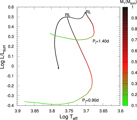
Figure 1: Hertzsprung-Russell diagram for the evolution of the initially 1.0 $M_{\sun}$ secondary star. The tracks corresponding to initial orbital periods of 0.90 and 1.40d are depicted. The final mass at the end of Roche lobe overflow is, respectively, 0.15540 and 0.18685 $M_{\sun}$. RL marks the locations in the diagram when the secondary star fills its Roche lobe for the first time and mass loss begins. The color scale to the right shows the stellar mass of the secondary star.

$$\frac{\dot{J}}{J}=\frac{\dot{J}_{ML}}{J}+\frac{\dot{J}_{GR}}{J}+\frac{\dot{J}_{MB}}{J}\,,$$ (1)

where $\dot{J}_{ML}$, $\dot{J}_{GR}$, and $\dot{J}_{MB}$, are respectively, the angular momemtum loss from the system due to mass loss, gravitational wave radiation and magnetic braking (which is relevant when the secondary has an outer convection zone). To compute these quantities we follow Sarna et al. (2000), see also Muslimov & Sarna (1993)

$$\frac{\dot{J}_{ML}}{J}=\frac{M_{2}}{M_{1}(M_{1}+M_{2})}{\dot{M}_{1}}\,{\rm yr^{-1}}.$$ (2)

$$\frac{\dot{J}_{GR}}{J}=-8.5\times 10^{-10}\frac{M_{1}M_{2}(M_{1}+M_{2})}{a^{4}}\,{\rm yr^{-1}},$$ (3)

$$\frac{\dot{J}_{MB}}{J}=-3\times 10^{-7}\frac{(M_{1}+M_{2})^{2}R^{4}_{1}}{M_{1}M_{2}a^{5}}\,{\rm yr^{-1}}\,,$$ (4)

where $a$ is the semiaxis of the orbit and $R_{1}$ the radius of the secondary. All quantities are given in solar units. The mass-loss rate from the secondary is calculated as in Chen & Han (2002). Mass loss is considered as long as the secondary fills its Roche lobe $r_{L}$, given by

$$r_{L}=a\frac{0.49q^{2/3}}{0.6q^{2/3}+\rm{ln}(1+q^{1/3})},$$ (5)

where $q=M_{1}/M_{2}$ is the mass ratio. The semiaxis of the orbit is found by integrating the equation for the rate of change of $a$, which in the case that the mass lost by the secondary is completely lost from the system, i.e. nothing of the mass lost by the secondary is accreted by the primary, is given by (see Muslimov & Sarna 1993)

$$\frac{1}{2}\frac{\dot{a}}{a}=\frac{\dot{J}}{J}-\left(\frac{1}{M_{1}}-\frac{1}{2(M_{1}+M_{2})}\right)\dot{M}_{1}$$ (6)

Mass loss is continued until the secondary star shrinks within its Roche lobe. It may happen that as a result of a hydrogen thermonuclear flash occurring on the white dwarf cooling branch, the secondary fills for the second time its Roche lobe during the flash. This being the case, mass loss becomes operative again on a very short timescale. We want to mention that the present treatment for mass loss is not completely self-consistent in the sense that the mass-loss rate is not considered as a unknown quantity during the iteration procedure to solve the stellar structure equations, but instead is fixed beforehand for each model. Nonetheless, it constitutes a better approach to derive physically sound initial ELM white dwarf models than arbitrarily removing mass to a evolving low-mass star. It is enough for the purpose of this work, the aim of which is focused on the cooling and structural properties of ELM white dwarfs.

All of our He-core white dwarf initial models have been derived from evolutionary calculations for binary systems consisting of an evolving low-mass component of initially $1\,M_{\sun}$ and a $1.4\,M_{\sun}$ neutron star as the other component. Metallicity is assumed to be Z=0.01. A total of 14 initial He-core white dwarf models with stellar masses between 0.155 and 0.435 $M_{\sun}$ have been derived for initial orbital periods at the beginning of the Roche lobe phase in the range 0.9 to 300 d. In particular, 9 sequences span the range of masses corresponding to ELM-white dwarfs ($M\lesssim 0.20M_{\sun}$). At this point, it is worth mentioning that the envelope mass of the resulting white dwarf, a key factor in dictating the cooling times, is only weakly dependent on the initial mass of the secondary (mass-losing) star (Nelson et al. 2004). However, different angular-momentum loss prescriptions due to mass loss, which could have an impact on the final envelope mass, have not been explored in this paper.

Figure 2: Surface gravity - effective temperature diagrams for our He-core white dwarf sequences. From left to right and from top to bottom, diagrams correspond to sequences of masses: 0.43523, 0.36304, 0.32079, 0.27242, 0.23903, 0.20258, 0.19210, 0.18685, 0.18213, 0.17624, 0.17064, 0.16499, 0.16115, 0.15540$M_{\sun}$. Sequences with masses in the range $0.18M_{\sun}\lesssim M_{\rm WD}\lesssim 0.4M_{\sun}$ undergo CNO flashes during the early cooling phase leading to the apparent loops in the $g$-$T_{\rm eff}$ diagram. Filled circles and triangles correspond, respectively, to the observed post-RGB low-mass stars from Silvotti et al. (2012) and Brown et al. (2013), and asteriks to the pulsating ELM white dwarfs detected by Hermes et al. (2013), see Table 2.

In Table 2, we provide some main characteristics of our whole set of initial He-core white dwarf models we have calculated. From left to right we list the stellar mass of the secondary star at the end of Roche lobe overflow ($M_{\rm f}(M_{\sun})$); the initial orbital period (in days) of the system at the beginning of the mass transfer phase ($P_{\rm i}$); the final orbital period (in days) at the end of Roche lobe overflow ($P_{\rm f}$); the surface hydrogen abundance (by mass) at the end of the Roche lobe overflow ($X_{\rm f}^{\rm surf}$), and the mass of the total hydrogen content at the point of maximum effective temperature at the beginning of the first cooling branch ($M_{\rm H}$). The further evolution of these initial models has been computed down to the range of luminosities of cool white dwarfs, including the stages of multiple thermonuclear CNO flashes during the beginning of cooling branch. The numbers between brackets in the first column denote the stellar mass of the remnant that is left after the occurrence of a second stage of Roche lobe overflow during the CNO flash. Indeed, during the course of the CNO flash, the white dwarf remnant may be forced to fill its Roche lobe again, thus leading to a new mass transfer episode. Note also from Table 2 that, in good agreement with previous studies (Sarna et al. 2000; Althaus et al. 2001) there exists a threshold in the stellar mass value (at $\sim 0.18M_{\sun}$), below which CNO flashes are not expected.

3 Evolutionary results

As an example of the evolution of the white dwarf progenitor during the mass transfer stage, we show in Fig. 1 the Hertzsprung-Russell diagram for the evolution of the initially 1.0 $M_{\sun}$ secondary star. Evolution of the secondary starts from the ZAMS and it is followed until the end of core hydrogen burning and the further stages. Two tracks are shown, which correspond to initial orbital periods of 0.90 and 1.40d. At the points denoted by RL, the secondary fills it Roche Lobe for the first time, and mass loss from the system begins. Note that from that moment on, the secondary evolves at almost constant radius, until its stellar mass decreases below $\sim$ 0.4 $M_{\sun}$. Mass loss continues until the secondary shrinks within its Roche lobe. The final mass at the end of Roche lobe overflow is, respectively, 0.15540 and 0.18685 $M_{\sun}$. The evolutionary tracks for our He-core white dwarf models start precisely after the end of Roche lobe overflow.

The evolution in the plane surface gravity versus effective temperature for all of our He-core white dwarf sequences is shown in Fig. 2, together with selected post-RGB low-mass objects presumably to be He-core white dwarfs (most of them ELM white dwarfs), see Table 2. In Fig. 3 we display on the same plot the results for the ELM sequences which do not experience CNO flashes on the cooling branch, together with the lowest mass He-core white dwarf sequence that experiences CNO flashes, the 0.18213 $M_{\sun}$ sequence (see Table 2). The figure illustrates the evolutionary stages corresponding to the first 7 Gyr of evolution after the end of mass loss. The main remarkable characteristic of the no-flashing sequences is their slow evolution over most of their life, which is due to the residual hydrogen shell burning being the main source of surface luminosity even at very advanced stages of evolution. In particular, for the least massive of our ELM sequences, evolutionary timescales involved in reaching the white dwarf cooling branch from the end of mass loss amount to about 1 Gyr, which means that these objects should have large chances of being observed during those stages. Also noticeable is the very slow rate of evolution at intermediate effective temperatures on the cooling branch. In fact, note that evolution takes about several Gyr in reaching $T_{\rm eff}\sim$ 9000K. And this is so because even at such advanced stages, stable hydrogen shell burning still provides the main energy source. It is clear that for these ELM white dwarfs, an appropriate treatment of progenitor evolution is required for a correct assessment of the evolutionary time scales.

By contrast, the behavior is entirely different for the sequences that do experience unstable hydrogen shell burning on their early cooling branch, as can appreciated by inspecting the track corresponding to the 0.18213 $M_{\sun}$ sequence in Fig. 3. This sequence experiences nine CNO flashes before reaching the quiescent terminal white-dwarf cooling branch. Several points are worthy of comment. Note that during the final cooling branch evolution proceeds on a timescale much shorter than that characterizing the sequences with $M<0.18M_{\sun}$. This is because CNO flashes markedly reduce the hydrogen content of the star, with the result that residual nuclear burning is much less relevant when the remnant reaches the final cooling branch. Hence, sequences that go through several episodes of CNO flashes are expected to evolve below $T_{\rm eff}=5000$K in a time much less than the Hubble time, in contrast with the situation for the least massive ELM sequences for which nuclear burning substantially delays their evolution by several Gyr at higher effective temperatures. This age dichotomy, which is the result of the interplay of element diffusion and nuclear burning during the flash episodes, is a remarkable property of very low mass He-core white dwarfs with important observational consequences, as we reported in previous investigations (see Althaus et al. 2001; Panei et al. 2007 and references therein).

It is worth noting that, in the case of CNO-flashing sequences, the rate of evolution slows down during the stages just prior to the occurrence of the CNO flashes on the early cooling branches. This is illustrated by Fig. 4, which shows the evolutionary speed of some selected CNO-flashing sequences in the $\log T_{\rm eff}-\log g$ diagram. The slower evolution just before the occurrence of the CNO flashes is apparent. Hence, the observational counterparts of these remnants could have chances of being detected also during these evolutionary stages. This should be taken into account when attempt is made at assessing the stellar mass and age of He-core white dwarfs from evolutionary sequences that experience several CNO flashes, since multiple solutions are, in principle, possible from such sequences, at intermediate effective temperatures (see Silvotti et al. 2012). This can be clearly understood by inspecting Fig. 2. We develop this issue in the next section.

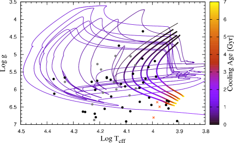
Figure 3: Surface gravity - effective temperature diagram for ELM white dwarf sequences with 0.15540, 0.16115, 0.16499, 0.17064, 0.17624 $M_{\sun}$ (thick lines, from right to left) together with the lowest mass He-core white dwarf sequence that undergoes CNO flashes (0.18213 $M_{\sun}$, thin line). Tracks correspond to the first 7 Gyr of evolution after the end of mass loss when the secondary shrinks within its Roche lobe. The color scale to the right displays the cooling age in Gyr. Note the much faster evolution of the 0.18213 $M_{\sun}$ sequence after the occurrence of the CNO flashes. Black and grey circles represent observed non-pulsating post-RGB low-mass stars, and red asteriks pulsating ELM white dwarfs, as detailed in Table 2.

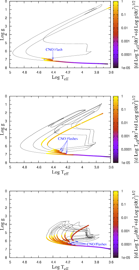
Figure 4: Evolutionary speed of the sequences in the $\log T_{\rm eff}-\log g$ diagram —for 0.36304 $M_{\sun}$, 0.27242, and 0.18213$M_{\sun}$ (top, middle, and bottom panels, respectively). Thin black lines denote evolutionary stages faster than the upper boundary of the color coding. Note the much faster evolution of the more massive sequences before entering the white dwarf cooling sequence.

4 Mass and Age determination

Our grid of He-core white dwarf sequences is appropriate for homegeneous mass and cooling age determinations of observed low-mass white dwarfs for all of the evolutionary stages where these stars have chances of being observed, i.e., the final cooling branch, the stages at constant luminosity following the end of Roche lobe overflow (particularly in the case of ELM white dwarfs), and, as we mention, the evolutionary stages prior to the occurrence of the CNO flashes on the early cooling branches. These evolutionary stages are highlighted in Fig. 4 for some selected CNO-flashing sequences. Because of the occurrence of several CNO flashes, special care must be taken at assessing the age and mass from theoretical He-core evolutionary sequences. Usually, white dwarf masses and cooling ages are derived from their $\log g$-$\log T_{\rm eff}$ values by means of theoretical white dwarf tracks and isochrones in the $\log g$-$\log T_{\rm eff}$ plane. Performing linear interpolation among available tracks and isochrones is usually enough to obtain masses and cooling ages directly from the $\log g$-$\log T_{\rm eff}$ values. However, in the case of low-mass He-core white dwarfs the problem is rather involved. As can be seen in Fig. 2 for high effective temperatures, He-core white dwarf tracks cross each other in the $\log g$-$\log T_{\rm eff}$ plane, leading to a multiplicity of the possible solutions, both for mass and cooling age, for a given measured value for $\log g$ and $\log T_{\rm eff}$. This multiplicity of the age and mass solutions would be almost irrelevant if the evolutionary stages at which the tracks cross each other (loops) were fast and consequently with a low probability to find a star at those stages. Unfortunately, the time spent during these loops is not negligible and, thus, several solutions are possible for a given measured value for $\log g$ and $\log T_{\rm eff}$. Consequently, the determination of masses and ages of He-core white dwarfs calls for some kind of statistical approach to weight the time spent by each model in each region of the $\log g$-$\log T_{\rm eff}$ diagram.

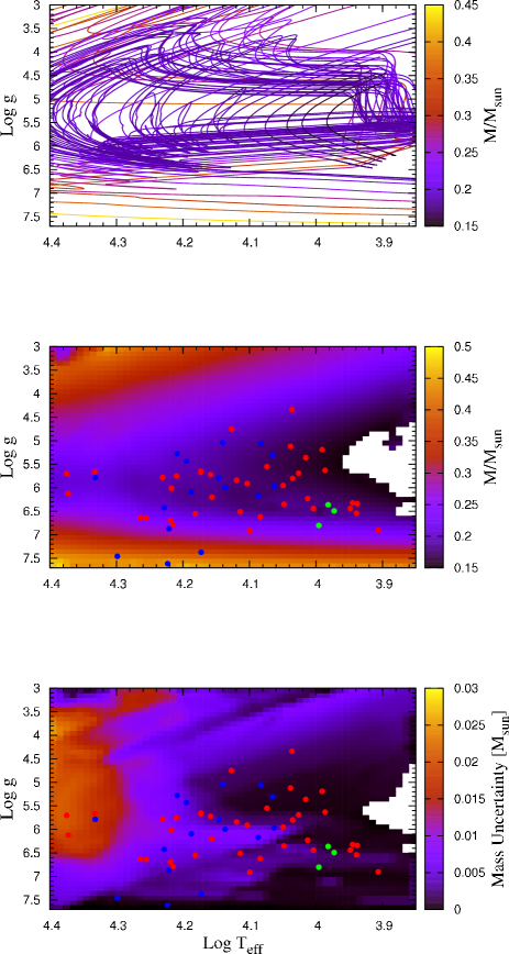
Figure 5: Top Panel: $M(\log T_{\rm eff},\log g)$ relation as obtained directly from stellar evolution simulations. Middle Panel: $M(\log T_{\rm eff},\log g)$ relation derived from the weighted least square scheme described in Sect. 4. Bottom Panel: Uncertainty $\sigma_{M}$ of the derived $M(\log T_{\rm eff},\log g)$ relation. Symbols correspond to the observed post-RGB low-mass stars listed in Table 2. In particular, green circles correspond to the pulsating ELM white dwarfs detected by Hermes et al. (2013). White regions in middle and bottom panels indicate either fast evolutionary stages for which not enough points were available to obtain an accurate fit (in the case of CNO-flashing sequences), or simply that no tracks are available at that regions.

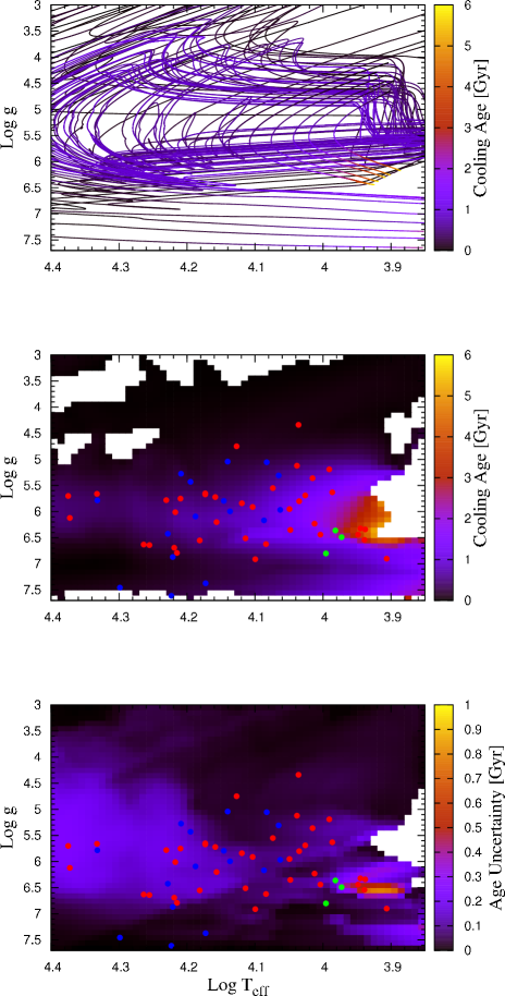
Figure 6: Same as Fig. 5 but for the $t(\log T_{\rm eff},\log g)$ relation and its corresponding uncertainty $\sigma_{t}$.

In this connection, we adopted the following scheme to determine masses and cooling ages of He-core white dwarfs from our sequences. In order to weight the time spent by each model at different locations of the $\log g$-$\log T_{\rm eff}$ diagram we created random values of cooling age $(t)$ and mass ($M_{*}$) and computed their corresponding theoretical values of $\log g$-$\log T_{\rm eff}$ from our sequences. Thus we are left with a set of points whose density in the $\log g$-$\log T_{\rm eff}$ diagram is directly related to the probability of finding a model of a given mass at that location of the $\log g$-$\log T_{\rm eff}$ diagram. Because interpolation between different tracks is not possible we adopted for each mass value that of our closest model. In the absence of a better knowledge of He-core white dwarf progenitor lifetimes and masses, we assumed a uniform distribution in mass and cooling age within the ranges $M_{*}\in(0.14965M_{\sun},0.50742M_{\sun})$ and $t\in(0{\rm Gyr},7{\rm Gyr})$. Within these assumptions we computed $2\times 10^{7}$ points to have a good sampling of the $\log g$-$\log T_{\rm eff}$-Mass-Age relationship. Then, for each observed He-core white dwarf star with known values of $\log g$-$\log T_{\rm eff}$ (see Table 2) we performed a least square polynomial fitting of the $\log g$-$\log T_{\rm eff}$-Mass-Age relationship within an ellipse around the ($\log g^{\rm star}$,$\log T_{\rm eff}^{\rm star}$) values of the star and derived its mass and age. We adopted the dispersion around the fitted polynom as an estimation of the errors in mass and cooling age. The size of the ellipse and the degree of the polynomial expression were chosen to allow for a good representation of different regions of the $\log g$-$\log T_{\rm eff}$ plane. Specifically, we adopted the following expressions. For the region where the “knees” of the tracks are located ($\log g<-12.1+4.5\times\log T_{\rm eff}$) we adopted

$$M(\log T_{\rm eff},\log g) = a\,\log^{2}T_{\rm eff}+b\,\log^{2}g+c\,\log T_{\rm eff}\,\log g$$ (7)

$$+ d\,\log T_{\rm eff}+e\,\log g+d.$$

For values of $\log g>-12.1+4.5\times\log T_{\rm eff}$, a first degree polynom was adopted.

$$M(\log T_{\rm eff},\log g)=a^{\prime}\,\log T_{\rm eff}+b^{\prime}\,\log g+c^{\prime}$$ (8)

Similar expressions were adopted in the same regions for the $t(\log T_{\rm eff},\log g)$ relation.

To select the points to be used in each fitting we adopted

$$\left(\frac{\log T_{\rm eff}-\log T_{\rm eff}^{\rm star}}{0.04\times\alpha}\right)^{2}+\left(\frac{\log g-\log g^{\rm star}}{0.6\times\beta}\right)^{2}\leq 1$$ (9)

Where $\alpha$ and $\beta$ have to be chosen in such a way to allow enough points for the least square fit but, at the same time, keeping them small enough so that the $t(\log T_{\rm eff},\log g)$ and $M(\log T_{\rm eff},\log g)$ can be reproduced by the simple polynomial expressions of Eq. 7 and 8. In particular $\alpha$ and $\beta$ were taken as

$$\alpha = 1.5,\,\beta=1.5,\ \hbox{if}\ \log g<-34.6+9.4\times\log T_{\rm eff}$$

$$\alpha = 1,\,\beta=1.5,$$

if $$-34.6+9.4\times\log T_{\rm eff}\leq\log g<-12.1+4.5\times\log T_{\rm eff}$$

$$\alpha = 1,\,\beta=0.5,$$

if $$-12.1+4.5\times\log T_{\rm eff}\leq\log g<-21.55+7\times\log T_{\rm eff}$$

$$\alpha = 1,\,\beta=0.325,\hbox{in any other case}.$$ (10)

In Figs. 5 and 6 we can see the $M(\log T_{\rm eff},\log g)$ and $t(\log T_{\rm eff},\log g)$ relations as given directly by our stellar evolution sequences (top panels) together with the weighted least square fitted $M(\log T_{\rm eff},\log g)$ and $t(\log T_{\rm eff},\log g)$ relations described above (middle panels) and the estimated uncertainties of the least squared fit procedure (bottom panel). It is worth noting that the relatively large uncertainties of the interpolated $M(\log T_{\rm eff},\log g)$ relation (Fig. 5, bottom panel) at $\log g\lesssim 6.5$ and $\log T_{\rm eff}\gtrsim 4.3$ is a natural consequence of the fact that sequences of different masses spend similar times in that region, making that region populated by stars of different masses. Hence, multiple solutions (with a dispersion of 0.03$M_{\sun}$) for the inferred stellar mass are possible at that region. A similar situation can be appreciated in the $t(\log T_{\rm eff},\log g)$ relation at $5.5\lesssim\log g\lesssim 6.5$ and $\log T_{\rm eff}\gtrsim 4.1$ where the uncertainty of the derived cooling ages is of about a few hundred Myrs. In addition, the $t(\log T_{\rm eff},\log g)$ relation becomes very uncertain ($\sigma_{t}\sim 1$Gyr) around $\log g\sim 6.5$ and $3.9\lesssim\log T_{\rm eff}\lesssim 3.95$. This feature is because at that region of the $\log g$-$\log T_{\rm eff}$ diagram it is expected the age dichotomy between the very low mass sequences ($M_{*}$$\lesssim$$0.18M_{\sun}$) which do not undergo CNO flashes (and, as we saw, evolve at a very slow pace) and the higher mass sequences ($M_{*}$$\gtrsim$$0.18M_{\sun}$) which undergo CNO flashes with the consequent much faster evolution during the final cooling branch.

Table 2: Selected post-RGB low-mass stars. Masses and cooling ages (fourth and fifth columns) are calculated from our sequences under the assumption that they are He-core white dwarfs. $\log g$ and $\log T_{\rm eff}$ values were taken from the tables of Silvotti et al. (2012, first 38 listed objects), Hermes et al. (2013, next 3 listed objects) and Brown et al. (2013, final 17 listed objects). The last two columns list the values as derived from our procedure for quick mass and age determination, see Sect. 4.1.

Name	Teff/K	log $g$ (cm s${}^{-2})$	M/M☉	Cooling Age [Myr]	Mapp/M☉	C. Ageapp [Myr]
V209 $\omega$ Cen	10866 $\pm$ 323	4.34 $\pm$ 0.02	0.202 $\pm$ 0.0021	55 $\pm$ 31	0.206	85
WASP J0247$-$25	13400 $\pm$1200	4.75 $\pm$ 0.05	0.203 $\pm$ 0.0019	110 $\pm$ 25	0.208	100
SDSS J1233+1602	10920 $\pm$ 160	5.12 $\pm$ 0.07	0.169 $\pm$ 0.0005	434 $\pm$ 50	0.172	547
SDSS J1741+6526	9790 $\pm$ 240	5.19 $\pm$ 0.06	0.159 $\pm$ 0.0003	712 $\pm$ 80	0.161	838
SDSS J2119$-$0018	10360 $\pm$ 230	5.36 $\pm$ 0.07	0.161 $\pm$ 0.0004	885 $\pm$ 90	0.162	935
SDSS J0917+4638	11850 $\pm$ 170	5.55 $\pm$ 0.05	0.170 $\pm$ 0.0003	703 $\pm$ 46	0.172	762
SDSS J0112+1835	9690 $\pm$ 150	5.63 $\pm$ 0.06	0.156 $\pm$ 0.0003	1604 $\pm$ 93	0.158	1653
KIC 10657664	14900 $\pm$ 300	5.65 $\pm$ 0.04	0.189 $\pm$ 0.0035	382 $\pm$ 116	0.189	421
HD 188112	21500 $\pm$ 500	5.66 $\pm$ 0.05	0.211 $\pm$ 0.0175	329 $\pm$ 207	0.212	291
GALLEX J1717	14900 $\pm$ 200	5.67 $\pm$ 0.05	0.188 $\pm$ 0.0039	406 $\pm$ 127	0.188	432
SDSS J0818+3536	10620 $\pm$ 380	5.69 $\pm$ 0.07	0.163 $\pm$ 0.0014	1263 $\pm$ 79	0.165	1383
KIC 06614501	23700 $\pm$ 500	5.70 $\pm$ 0.10	0.210 $\pm$ 0.0209	368 $\pm$ 239	0.217	287
KOI 1224	14400 $\pm$1100	5.72 $\pm$ 0.05	0.186 $\pm$ 0.0024	441 $\pm$ 82	0.186	474
NGC 6121 V46	16200 $\pm$ 550	5.75 $\pm$ 0.11	0.191 $\pm$ 0.0064	450 $\pm$ 176	0.192	435
KOI 81	17000 $\pm$1300	5.78 $\pm$ 0.13	0.196 $\pm$ 0.0072	372 $\pm$ 186	0.194	427
SDSS J0152+0749	10840 $\pm$ 270	5.80 $\pm$ 0.06	0.167 $\pm$ 0.0020	1312 $\pm$ 88	0.167	1461
SDSS J0755+4906	13160 $\pm$ 260	5.84 $\pm$ 0.07	0.178 $\pm$ 0.0027	633 $\pm$ 108	0.179	687
SDSS J1422+4352	12690 $\pm$ 130	5.91 $\pm$ 0.07	0.177 $\pm$ 0.0025	776 $\pm$ 95	0.177	817
SDSS J1630+2712	11200 $\pm$ 350	5.95 $\pm$ 0.07	0.171 $\pm$ 0.0023	1270 $\pm$ 89	0.171	1302
SDSS J0106–1000	16490 $\pm$ 460	6.01 $\pm$ 0.04	0.186 $\pm$ 0.0099	568 $\pm$ 174	0.193	524
SDSS J1625+3632	23570 $\pm$ 440	6.12 $\pm$ 0.03	0.214 $\pm$ 0.0188	415 $\pm$ 212	0.220	304
SDSS J1439+1002	14340 $\pm$ 240	6.20 $\pm$ 0.07	0.182 $\pm$ 0.0070	746 $\pm$ 125	0.186	705
SDSS J0849+0445	10290 $\pm$ 250	6.23 $\pm$ 0.08	0.178 $\pm$ 0.0003	1780 $\pm$ 34	0.176	1877
SDSS J1443+1509	8810 $\pm$ 220	6.32 $\pm$ 0.07	0.173 $\pm$ 0.0004	3646 $\pm$ 200	0.172	4037
PSR J1012+5307	8670 $\pm$ 300	6.34 $\pm$ 0.20	0.172 $\pm$ 0.0004	4034 $\pm$ 169	0.172	4341
LP 400-22	11170 $\pm$ 90	6.35 $\pm$ 0.05	0.182 $\pm$ 0.0025	1195 $\pm$ 100	0.182	1279
PSR J1911$-$5958	10090 $\pm$ 150	6.44 $\pm$ 0.20	0.185 $\pm$ 0.0041	1471 $\pm$ 167	0.184	2324
SDSS J0822+2753	8880 $\pm$ 60	6.44 $\pm$ 0.11	0.178 $\pm$ 0.0010	3255 $\pm$ 416	0.179	3862
KOI 74	13000 $\pm$1000	6.51 $\pm$ 0.10	0.186 $\pm$ 0.0016	930 $\pm$ 64	0.197	670
NLTT 11748	8690 $\pm$ 140	6.54 $\pm$ 0.05	0.183 $\pm$ 0.0020	2572 $\pm$ 507	0.184	3011
SDSS J1053+5200	15180 $\pm$ 600	6.55 $\pm$ 0.09	0.204 $\pm$ 0.0045	479 $\pm$ 147	0.213	412
SDSS J1512+2615	12130 $\pm$ 210	6.62 $\pm$ 0.07	0.198 $\pm$ 0.0034	750 $\pm$ 76	0.205	683
SDSS J0923+3028	18350 $\pm$ 290	6.63 $\pm$ 0.05	0.238 $\pm$ 0.0067	188 $\pm$ 112	0.246	178
SDSS J1234$-$0228	18000 $\pm$ 170	6.64 $\pm$ 0.03	0.235 $\pm$ 0.0063	225 $\pm$ 124	0.245	194
SDSS J1436+5010	16550 $\pm$ 260	6.69 $\pm$ 0.07	0.234 $\pm$ 0.0047	230 $\pm$ 126	0.240	264
SDSS J0651+2844	16400 $\pm$ 300	6.79 $\pm$ 0.04	0.248 $\pm$ 0.0041	196 $\pm$ 107	0.260	262
PSR J0218+4232	8060 $\pm$ 150	6.90 $\pm$ 0.70	0.227 $\pm$ 0.0001	1162 $\pm$ 48	0.237	1505
SDSS J1448+1342	12580 $\pm$ 230	6.91 $\pm$ 0.07	0.250 $\pm$ 0.0030	302 $\pm$ 13	0.263	525
SDSS J1112+1117	9590 $\pm$ 140	6.36 $\pm$ 0.06	0.179 $\pm$ 0.0012	2756 $\pm$ 218	0.178	3061
SDSS J1840+6423	9390 $\pm$ 140	6.49 $\pm$ 0.06	0.183 $\pm$ 0.0018	1926 $\pm$ 453	0.184	2766
SDSS J1518+0658	9900 $\pm$ 140	6.80 $\pm$ 0.05	0.220 $\pm$ 0.0013	733 $\pm$ 33	0.224	829
J0840+1527	13810 $\pm$ 240	5.043 $\pm$ 0.053	0.193 $\pm$ 0.0018	181 $\pm$ 23	0.200	199
J1157+0546	12100 $\pm$ 250	5.054 $\pm$ 0.071	0.180 $\pm$ 0.0008	263 $\pm$ 32	0.185	323
J1238+1946	16170 $\pm$ 260	5.275 $\pm$ 0.051	0.199 $\pm$ 0.0064	233 $\pm$ 157	0.205	225
J1141+3850	11620 $\pm$ 200	5.307 $\pm$ 0.054	0.171 $\pm$ 0.0005	526 $\pm$ 55	0.173	584
J0751-0141	15660 $\pm$ 240	5.429 $\pm$ 0.046	0.200 $\pm$ 0.0053	223 $\pm$ 137	0.196	287
J0815+2309	21470 $\pm$ 340	5.783 $\pm$ 0.046	0.207 $\pm$ 0.0171	373 $\pm$ 198	0.208	333
J0811+0225	13990 $\pm$ 230	5.794 $\pm$ 0.054	0.183 $\pm$ 0.0028	528 $\pm$ 104	0.183	542
J1538+0252	11560 $\pm$ 220	5.967 $\pm$ 0.053	0.172 $\pm$ 0.0056	1155 $\pm$ 89	0.173	1184
J2132+0754	13700 $\pm$ 210	5.995 $\pm$ 0.045	0.176 $\pm$ 0.0080	732 $\pm$ 125	0.181	725
J1151+5858	15400 $\pm$ 300	6.092 $\pm$ 0.057	0.183 $\pm$ 0.0072	647 $\pm$ 147	0.188	628
J0056-0611	12210 $\pm$ 180	6.167 $\pm$ 0.044	0.175 $\pm$ 0.0078	982 $\pm$ 77	0.176	1055
J0802-0955	16910 $\pm$ 280	6.423 $\pm$ 0.048	0.206 $\pm$ 0.0063	361 $\pm$ 158	0.213	347
J2338-2052	16630 $\pm$ 280	6.869 $\pm$ 0.050	0.263 $\pm$ 0.0040	168 $\pm$ 99	0.279	242
J1046-0153	14880 $\pm$ 230	7.370 $\pm$ 0.045	0.376 $\pm$ 0.0055	224 $\pm$ 29	0.381	269
J0755+4800	19890 $\pm$ 350	7.455 $\pm$ 0.057	0.422 $\pm$ 0.0008	104 $\pm$ 3	0.420	99
J1104+0918	16710 $\pm$ 250	7.611 $\pm$ 0.049	0.455 $\pm$ 0.0001	158 $\pm$ 3	0.442	182
J1557+2823	12550 $\pm$ 200	7.762 $\pm$ 0.046	0.456 $\pm$ $<$0.0001	541 $\pm$ 1	0.460	415

As an application of our He-core white dwarf sequences and the above described interpolation algorithm, we have determined the stellar masses and cooling ages for the sample of post-RGB low-mass stars (most of them ELM white dwarfs) listed in Silvotti et al. (2012) and in Brown et al. (2013). We assume that these stars have a He core. The derived values of mass and cooling age for each star is shown in Table 2 together with the estimated uncertainties (fourth and fifth columns). We mention that for such white dwarfs, the age values listed in Table 2 constitute the first assessment of their cooling ages. As a check, we compare our derived values with those derived by the standard interpolation approach, which can be performed for white dwarfs with masses $M_{*}<0.18M_{\sun}$, and found that the difference in the masses and ages is well within the quoted uncertainties. We want to mention that some differences appear between the inferred stellar mass from our sequences and stellar mass values quoted by Silvotti et al (2012) and Brown et al. (2013). This is particularly true in the case of the ELM white dwarf sample of Brown et al. (2013), who, for most of their sample, found a stellar mass value of $0.17M_{\sun}$, in contrat with our analysis, which yields stellar mass values in the range 0.17$M_{\sun}$ - 0.21$M_{\sun}$. This difference is due to the fact that Brown et al. (2013) adopted the final cooling track (after all the flashes) as the representative one for the sequences which undergo CNO-flashes. As shown in Fig. 4, it is the first entrance to the white dwarf cooling phase which is slower and takes longer time. Thus, for sequences which undergo CNO flashes it is more probable to find a star of a given mass during its first entrance (which occurs at lower effective temperatures) than during its final entrance to the white dwarf cooling zone. Choosing the final cooling track to derive masses at gravities $\log g\lesssim 6$ leads to an underestimation of the stellar mass of up to 20%. Note that the differences in the evolutionary speeds of different sequences is naturally taken into account in the scheme presented in the previous section.

We also checked the estimations performed by the scheme presented here by comparing our results with the analysis performed by Silvotti et al. (2012) on KIC 6614501. By assuming that the binary component is a He-core white dwarf they discussed two possibilities: i) its mass is $M_{1}\sim 0.185M_{\odot}$ and the star is on the final cooling track after all the CNO flashes, which occurs at a faster pace and it is thus less probable (see Fig. 4.) and ii) its mass is $M_{1}\gtrsim 0.19M_{\odot}$ and the star is still on one of the cooling branches during the CNO-flash stage. In the second case the mass of the star should be constrained between 0.19$-$0.24 $M_{\odot}$, from a comparison with Althaus et al. (2001) tracks and the cooling age should be between 30 and 290 Myr. On the first, and less probable case, the age derived by Silvotti et al. (2012) is of 180 Myr. By looking at Table 2 we see that our mass and cooling age determination scheme gives a value of $M_{1}=0.210\pm 0.0209M_{\odot}$ and $t_{\rm age}=368\pm 239$ Myr for KIC 6614501. Then our mass derivation is in very good agreement with the values derived for option ii of Silvotti et al. (2012) and the same happens for the cooling age of the star. Note, in particular, that the large derived uncertainty in the mass and age within our approach is due to the fact that many different tracks go through that region of the $\log g$-$\log T_{\rm eff}$ plane at similar paces and, consequently a better determination of mass and age just from $\log g$ and $\log T_{\rm eff}$ is not possible.

4.1 A quick way to assess mass and cooling age of He-core white dwarfs

In order to provide other authors with an easy way to estimate the masses and cooling ages of He-core white dwarf stars from our tracks, we computed $M_{*}$ and $t$ with the previously described algorithm at a small grid of points in the $\log g$-$\log T_{\rm eff}$ diagram. Such a grid is presented in Table 3 and can be used via direct bilinear interpolation to obtain the masses and cooling ages at any point in the $\log g$-$\log T_{\rm eff}$ diagram. Because the grid is not regularly spaced in $\log T_{\rm eff}$ (for the sake of economy), interpolation must be performed first in $\log T_{\rm eff}$ and then in $\log g$. As an example, the results from these approximated estimations are listed in columns sixth and seventh of Table 2 and compared with those directly computed from the scheme presented in the previous section. While some differences are present in the derived cooling ages between the full scheme and the bilinear interpolation of Table 3, these differences are moderate and similar to the quoted uncertainties. In particular, for the ELM KIC 6614501 analysed by Silvotti et al. (2012), a simple bilinear interpolation from Table 3 gives straightforwardly $M_{1}\sim$0.217 $M_{\odot}$ and $t_{\rm age}\sim$287 Myr, very similar to the values derived by Silvotti et al. (2012). On the other hand, masses derived by the bilinear interpolation of the grid presented in Table 3 are in excellent agreement by those derived from the full scheme. Globally, bilinear interpolation of the values presented in Table 3 allows a very fast and easy way to derive masses and cooling ages for He-core white dwarfs. It should be noted however that, in the case of the age derivation, the bilinear interpolation within the rather coarse grid of Table 3 does not offer a good representation for those stars close to the age dichotomy that appears at higher gravities and lower temperatures. For those stars a more precise cooling age and mass derivation as those presented in Sect. 4 can be inferred from direct interpolation of the terminal cooling branch of our evolutionary sequences.

5 Prospects for an asteroseismic tool

Table 3: Masses and cooling ages at a grid in the log($g$)-log T_eff plane.

log Teff/K	log($g$/cm s${}^{-2})$	M/M☉	Cooling Age [Myr]
3.92	4.00	0.191 $\pm$ 0.0019	19 $\pm$ 27
4.00	4.00	0.215 $\pm$ 0.0032	54 $\pm$ 24
4.03	4.00	0.225 $\pm$ 0.0038	56 $\pm$ 14
4.20	4.00	0.278 $\pm$ 0.0041	8 $\pm$ 25
4.40	4.00	0.346 $\pm$ 0.0267	3 $\pm$ 125
3.92	4.70	0.158 $\pm$ 0.0004	109 $\pm$ 21
4.00	4.70	0.174 $\pm$ 0.0009	122 $\pm$ 33
4.03	4.70	0.181 $\pm$ 0.0013	119 $\pm$ 30
4.20	4.70	0.232 $\pm$ 0.0056	51 $\pm$ 76
4.50	4.70	0.296 $\pm$ 0.0257	42 $\pm$ 155
3.99	5.40	0.156 $\pm$ 0.0003	1151 $\pm$ 115
4.10	5.40	0.176 $\pm$ 0.0004	430 $\pm$ 34
4.15	5.40	0.187 $\pm$ 0.0016	302 $\pm$ 49
4.30	5.40	0.218 $\pm$ 0.0160	202 $\pm$ 200
4.50	5.40	0.242 $\pm$ 0.0307	202 $\pm$ 241
3.96	5.80	0.156 $\pm$ 0.0007	2300 $\pm$ 53
4.10	5.80	0.176 $\pm$ 0.0020	734 $\pm$ 76
4.15	5.80	0.184 $\pm$ 0.0029	528 $\pm$ 105
4.30	5.80	0.202 $\pm$ 0.0152	356 $\pm$ 187
4.50	5.80	0.235 $\pm$ 0.0301	245 $\pm$ 243
3.90	6.10	0.155 $\pm$ 0.0002	4532 $\pm$ 129
4.05	6.10	0.173 $\pm$ 0.0064	1284 $\pm$ 86
4.15	6.10	0.182 $\pm$ 0.0079	727 $\pm$ 133
4.30	6.10	0.207 $\pm$ 0.0129	345 $\pm$ 156
4.50	6.10	0.240 $\pm$ 0.0295	255 $\pm$ 233
3.91	6.25	0.163 $\pm$ 0.0002	4848 $\pm$ 124
4.00	6.25	0.177 $\pm$ 0.0004	1980 $\pm$ 48
4.10	6.25	0.175 $\pm$ 0.0074	879 $\pm$ 89
4.30	6.25	0.219 $\pm$ 0.0119	256 $\pm$ 159
4.50	6.25	0.249 $\pm$ 0.0286	236 $\pm$ 233
3.93	6.40	0.174 $\pm$ 0.0004	4847 $\pm$ 129
4.05	6.40	0.185 $\pm$ 0.0052	1132 $\pm$ 125
4.15	6.40	0.187 $\pm$ 0.0056	547 $\pm$ 152
4.30	6.40	0.232 $\pm$ 0.0108	181 $\pm$ 149
4.50	6.40	0.262 $\pm$ 0.0230	157 $\pm$ 184
3.80	6.70	0.180 $\pm$ 0.0006	2222 $\pm$ 22
4.00	6.70	0.202 $\pm$ 0.0018	799 $\pm$ 49
4.15	6.70	0.221 $\pm$ 0.0032	429 $\pm$ 62
4.30	6.70	0.264 $\pm$ 0.0086	60 $\pm$ 86
4.50	6.70	0.310 $\pm$ 0.0076	51 $\pm$ 32
3.80	7.43	0.347 $\pm$ 0.0020	2546 $\pm$ 102
4.00	7.43	0.369 $\pm$ 0.0033	786 $\pm$ 107
4.15	7.43	0.391 $\pm$ 0.0031	289 $\pm$ 31
4.30	7.43	0.415 $\pm$ 0.0009	96 $\pm$ 3
4.40	7.43	0.435 $\pm$ 0.0050	45 $\pm$ 8

We have carried out exploratory computations of the $g$-mode adiabatic pulsation properties of our ELM white dwarf models, in particular for sequences with stellar masses near the critical mass for the development of CNO flashes ($M_{*}\approx 0.2M_{\sun}$). This is motivated by the fact that at least two of the three ELM pulsating white dwarfs reported by Hermes et al. (2013) have stellar masses near this threshold value. A full exploration of the adiabatic and nonadiabatic pulsation properties of our complete set of low-mass and ELM white dwarfs is underway and will be presented in a future paper. Our pulsation computations have been performed with the Newton-Raphson nonradial pulsation code described in Córsico & Althaus (2006). Here, we focus on the most massive ELM sequence which does not experience CNO flashes on the cooling branch ($M_{*}=0.1762M_{\sun}$), and the lowest mass ELM white dwarf sequence that experiences CNO flashes ($M_{*}=0.1805M_{\sun}$). In Figs. 7 and 8 we display the chemical profiles and the propagation diagrams for two models at $T_{\rm eff}\sim 9\,500$ K. It is quite noteworthy that, being the difference in the stellar mass of these two models almost negligible ($\Delta M_{*}=0.0043M_{\sun}$), the internal chemical distribution is very different. In particular, the $M_{*}=0.1762M_{\sun}$ model has a pure H envelope that is $\sim 65$ times thicker than the $M_{*}=0.1805M_{\sun}$ model. Also, the shape of the He/H transition region is markedly different in both cases. Indeed, for the more massive model this chemical interface is still characterized by a double-layered structure, while for the less massive model it has already attained a single-layered structure due to the action of element diffusion. This markedly different behavior is a signature of the occurrence of CNO flashes in the $0.1805M_{\sun}$ sequence, and can be understood by examining Fig. 3. In fact, as a result of the less important role of residual H burning after the occurrence of the CNO flashes, the 0.18213 $M_{\sun}$ sequence evolves much faster than the $0.1762M_{\sun}$ sequence. Hence, the chemical profile in the 0.18213 $M_{\sun}$ sequence is not expected to be completely separated out by diffusion processes, as in the case of the less massive sequence.

The differences in the shape of the He/H interface for both models are translated into distinct features in the run of the squared critical frequencies, in particular in the Brunt-Väisälä frequency ($N^{2}$), as can be appreciated in Figs. 7 and 8, which depict also the propagation diagrams (Unno et al. 1989) corresponding to these models. In fact, for the $M_{*}=0.1805M_{\sun}$ model, $N^{2}$ is characterized by two bumps, as it is expected for a double-layered chemical structure at the He/H. At variance with this, for the $M_{*}=0.1762M_{\sun}$ model the Brunt-Väisälä frequency has only one bump, located at $\log(1-M_{r}/M_{*})\sim-1.9$, which is notoriously more pronounced than its counterpart in the $M_{*}=0.1805M_{\sun}$ model.

In pulsating stars in general, the structure of the $g$-mode period spectrum is sensitive to the spatial run of the Brunt-Väisälä frequency. This is particularly true for pulsating white dwarfs, in which the bumps of $N^{2}$ induced by chemical gradients are responsible for mode-trapping effects (Bradley 1996; Córsico et al. 2002). A clear signature of mode trapping is that the forward period spacing, defined as $\Delta\Pi_{k}(\equiv\Pi_{k+1}-\Pi_{k}$), when plotted in terms of the pulsation period $\Pi_{k}$, exhibits strong departures from uniformity. The period difference between an observed mode and adjacent modes ($\Delta k\pm 1$) can be used as an observational diagnostic of mode trapping. For stellar models characterized by a single chemical interface, like the one of $M_{*}=0.1762M_{\sun}$ we are considering here, local minima in $\Delta\Pi_{k}$ usually correspond to modes trapped in the H envelope, whereas local maxima in $\Delta\Pi_{k}$ are associated to modes trapped in the core region. In Fig. 9 we show the forward period spacing in terms of the dipole periods for the same models with $M_{*}=0.1762M_{\sun}$ and $M_{*}=0.1805M_{\sun}$ described in Figs. 7 and 8. We depict with a red horizontal line the asymptotic period spacing, computed as in Córsico et al. (2012). From this figure, mode-trapping signatures are clearly noticeably for both models, particularly for periods shorter than $\sim 2500$ s. Longer periods seem to fit the asymptotic predictions, although small departures from constant period spacing are still appreciable.

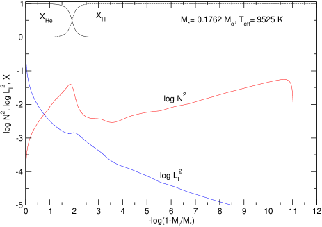
Figure 7: The internal chemical profiles of He and H and the propagation diagram —the run of the logarithm of the squared Brunt-Väisälä and Lamb (with $\ell=1$) frequencies— corresponding to an $0.1762M_{\sun}$ ELM white dwarf model at $T_{\rm eff}$$\sim$$9\,500$ K.

Focusing on the non-asymptotic regime ($\Pi_{k}\lesssim 2500$ s), we found appreciable differences in the period-spacing distributions of the two models. This, in spite of the fact that both models have virtually the same stellar mass. In particular, for the $M_{*}=0.1805M_{\sun}$ model the amplitude of the departure from uniform period spacing due to mode trapping is appreciably larger than for the $M_{*}=0.1762M_{\sun}$ one. Notably, this could be thought as a useful seismic tool for discriminating stars that have undergone CNO flashes in their early cooling phase from those that have not, provided that enough consecutive low- and intermediate-order ($200\lesssim\Pi\lesssim 2000$ s) $g$-modes with the same $\ell$ value were detected in pulsating ELM white dwarfs. At least two of the pulsating ELM white dwarfs reported by Hermes et al. (2013), with stellar mass near the threshold value for the occurrence of CNO flashes are potential candidates to test these ideas.

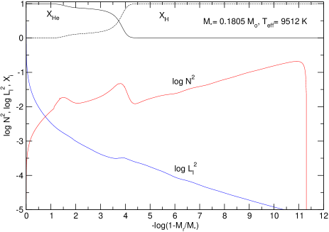
Figure 8: Same as in Fig. 7, but for a $0.1805M_{\sun}$ ELM white dwarf model.

6 Conclusions

In view of the discovery of numerous Extremely Low Mass (ELM) white dwarfs from different surveys (Brown et al. 2012, 2013 and references therein) and the recent detection of pulsations in some of them (Hermes et al. 2012, 2013), we present in this paper a detailed grid of evolutionary sequences for He-core white dwarfs by considering the binary evolution that leads to their formation. These new evolutionary models are intended for homogeneous mass and cooling age determinations as well as for potential asteroseismological applications of these stars.

Evolutionary calculations have been done with the amply used and well tested LPCODE stellar evolutionary code, appropriately modified to simulate the binary evolution of progenitor stars. Binary evolution has been assumed to be fully non-conservative, and the loss of angular momemtum due to mass loss, gravitational wave radiation and magnetic braking has been assumed. All of our He-core white dwarf initial models have been derived from evolutionary calculations for binary systems consisting of an evolving low-mass component of initially $1\,M_{\sun}$ and a $1.4\,M_{\sun}$ neutron star as the other component. Metallicity is assumed to be Z=0.01. A total of 14 initial He-core white dwarf models with stellar masses between 0.155 and 0.435 $M_{\sun}$ have been computed for initial orbital periods at the beginning of the Roche lobe phase in the range 0.9 to 300 d, see Table 2. In particular 9 sequences span the range of masses corresponding to ELM-white dwarfs ($M\lesssim 0.20M_{\sun}$). It should be mentioned that in this paper we have not considered different values of the initial mass of the secondary (mass-losing) star. Although it is expected that the envelope mass of the resulting white dwarf, a key factor in dictating the cooling times, is only weakly dependent on the initial mass of the mass-losing star (Nelson et al. 2004), different orbital angular-momentum loss prescriptions due to mass loss could have an impact on the final envelope mass. This issue has not been considered in this paper. Neither have we explored other physical processes, such as pulsar irradiation, which could reduce the resulting envelope mass of the He-core white dwarf (Ergma et al. 2001).

In agreement with previous studies, we found that for stellar masses larger than about 0.18 $M_{\sun}$, multiple CNO flashes are expected. Because of this, special care must be taken at assessing the cooling age and mass from evolutionary sequences, since multiple solutions are, in principle, possible from such sequences, at intermediate effective temperatures. To get realiable mass and cooling age determination from our sequences (given the surface gravity and effective temperature), we devised an interpolation algorithm that accounts for precisely the several possible solutions for stellar mass and cooling age in the case of the CNO-flashing sequences. As an application of our He-core white dwarf sequences, we have determined the stellar masses and cooling ages for the sample of post RGB low-mass stars considered in Silvotti et al. (2012) and Brown et al. (2013). Finally, we provide a simple scheme with the aim that our evolutionary sequences can be straightforwardly used for mass and age inferences of He-core white dwarfs.

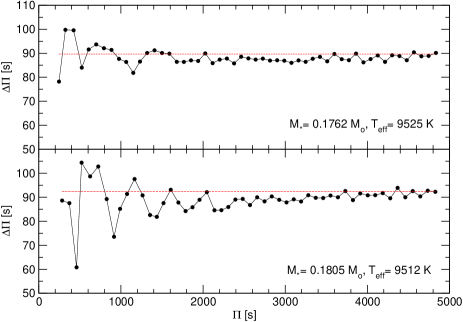
Figure 9: The forward period spacing in terms of the ($\ell$=$1$) periods for the model with $M_{*}$=$0.1762M_{\sun}$ (upper panel) and $M_{*}$=$0.1805M_{\sun}$ (lower panel), and a $T_{\rm eff}$$\sim$$9\,500$ K. The red horizontal line corresponds to the asymptotic period spacing.

Finally, we have explored the pulsation properties of ELM white dwarf models for sequences with stellar masses near the critical mass for the development of CNO flashes ($\sim 0.2M_{\sun}$). This has been motivated by the fact that at least two of the three ELM pulsating white dwarfs reported by Hermes et al. (2013) have stellar masses near this threshold value. Specifically, we have compared the period spacings of a model with $M_{*}=0.1762M_{\sun}$, corresponding to the most massive ELM sequence which does not experience CNO flashes on the cooling branch, with the period spacings of a model with $M_{*}=0.1805M_{\sun}$, corresponding to the lowest mass He core white dwarf sequence that experiences CNO flashes. Despite the small difference in their stellar masses, we have found that these models have appreciably different internal chemical structures, which impact quite differently on the mode trapping properties of the models for periods shorter than about $2500$ s. So, we can envisage an asteroseismic diagnostic tool for distinguishing stars that have undergone CNO flashes in their early cooling phase from those that have not, provided that enough consecutive pulsation periods of $g$-modes with low- and intermediate radial orders and the same harmonic degree were detected in pulsating ELM white dwarfs.

Finally, although the cooling age and mass of observed He-core white dwarfs can be directly inferred from the information provided in this paper, the complete set of our evolutionary sequences can be found at our web site http://www.fcaglp.unlp.edu.ar/evolgroup.

- (1) Althaus, L. G., Serenelli, A. M., & Benvenuto, O. G., 2001, MNRAS, 323, 471
- Althaus et al. (2010a) Althaus, L. G., Córsico, A. H., Isern, J., & García–Berro, E. 2010a, A&A Rev., 18, 471
- (3) Althaus, L. G., Serenelli, A. M., Córsico, A. H., Montgomery, M. H., 2003, A&A, 404, 593
- (4) Althaus, L. G., García–Berro, E., Isern, J., Córsico, A. H., & Miller Bertolami, M. M., 2012, A&A, 537, 33
- Althaus et al. (2007) Althaus, L. G., García–Berro, E., Isern, J., Córsico, A. H., & Rohrmann, R. D. 2007, A&A, 465, 249
- (6) Althaus, L. G., Serenelli, A. M., Panei, J. A., Córsico, A. H., García–Berro, E., & Scóccola, C. G., 2005, A&A, 435, 631
- Althaus et al. (2010) Althaus, L. G., Córsico, A. H., Bischoff-Kim, A., Romero, A. D., Renedo, I., García-Berro, E., & Miller Bertolami, M. M., 2010b, ApJ, 717, 897
- (8) Angulo, C., et al. 1999, Nuclear Physics A, 656, 3
- (9) Benvenuto, O. G., & De Vito, M. A., 2005, MNRAS, 362, 891
- (10) Bono, G., Salaris, M., & Gilmozzi, R., 2013, A&A, 549, A102
- (11) Bradley, P. A. 1996, ApJ, 468, 350
- (12) Brown, W. R., Kilic, M., Allende Prieto, C., & Kenyon S., 2010, ApJ, 723, 1072
- (13) Brown, W. R., Kilic, M., Allende Prieto, C., & Kenyon S., 2012, ApJ, 744, 142
- Cassisi et al. (2007) Cassisi, S., Potekhin, A. Y., Pietrinferni, A., Catelan, M., & Salaris, M. 2007, ApJ, 661, 1094
- (15) Chen, X., & Han, Z., 2002, MNRAS, 335, 948
- (16) Córsico, A. H., & Althaus, L. G. 2006, A&A, 454, 863
- (17) Córsico, A. H., Althaus, L. G., Miller Bertolami, M. M., et al. 2012a, MNRAS, 424, 2792
- (18) Córsico, A. H., Althaus, L. G., Romero, A. D., et al. 2012b, JCAP, 12, 10
- (19) Córsico, A. H., Romero, A. D., Althaus, L. G., & Hermes, J. J., 2012, A&A, 547, A96
- (20) Córsico, A. H., Althaus, L. G., Benvenuto, O. G., & Serenelli, A. M. 2002, A&A, 387, 531
- (21) Driebe, T., Schönberner, D., Blöcker, T., & Herwig, F., 1998, A&A, 339, 123
- (22) Ergma, E., Sarna, M. J., & Gerskevits-Antipova, J., 2001, MNRAS, 321, 71
- (23) Ferguson, J. W., Alexander, D. R., Allard, F., Barman T., Bodnarik, J. G., Hauschildt, P. H., Heffner-Wong, A., & Tamanai, A., 2005, ApJ, 623, 585
- (24) Fontaine, G., & Brassard, P., 2008, PASP, 120, 1043
- Garcia-Berro et al. (1995) García–Berro, E., Hernanz, M., Isern, J., & Mochkovitch, R. 1995, MNRAS, 277, 801
- García-Berro et al. (2010) García–Berro, E., Torres, S., Althaus, L. G., et al. 2010, Nature, 465, 194
- García-Berro et al. (2011) García–Berro, E., Lorén–Aguilar, P., Torres, S., Althaus, L. G., & Isern, J. 2011, J. Cosmology Astropart. Phys., 5, 21
- (28) Gautschy, A., 2013, arXiv:1303.6652
- Hansen et al. (2007) Hansen, B. M. S., Anderson, J., Brewer, J., et al. 2007, ApJ, 671, 380
- (30) Hermes, J. J., Montgomery, M. H., Winget, D. E., et al., 2012, ApJL, 750, L28
- (31) Hermes, J. J., Montgomery, M. H., Winget, D. E., et al., 2013, ApJ, 765, 102
- Iglesias & Rogers (1996) Iglesias, C. A., & Rogers, F. J. 1996, ApJ, 464, 943
- Isern et al. (1992) Isern, J., Hernanz, M., & García–Berro, E. 1992, ApJ, 392, L23
- Isern et al. (2008) Isern, J., García–Berro, E., Torres, S., & Catalán, S. 2008, ApJ, 682, L109
- (35) Kepler, S. O., Kleinman, S. J., Nitta, A., Koester, D., Castanheira, B. G., Giovannini, O., Costa, A. F. M., & Althaus, L. G, 2007, MNRAS, 375, 1315
- (36) Koester, D., Voss, B., Napiwotzki, R., Christlieb, N., Homeier, D., Lisker, T., Reimers, D., & Heber, U., 2009, A&A, 505, 441
- (37) Magni, G. & Mazzitelli, I., 1979, A&A, 72, 134
- (38) Maxted, P. F. L., Anderson, D. R., Burleigh, M. R., et al., 2011, MNRAS, 418, 1156
- (39) Miller Bertolami, M. M., Althaus, L. G., Olano, C., & Jiménez, N., 2011a, MNRAS, 415, 1396
- (40) Miller Bertolami, M. M., Althaus, L. G., Unglaub, K., & Weiss, A., 2008, A&A, 491, 253
- (41) Miller Bertolami, M. M., Rohrmann, R. D., Granada, A., & Althaus, L. G., 2011b, ApJ, 743, L33
- (42) Muslimov, A. G., & Sarna, M. J. ,1993, MNRAS, 262, 164
- (43) Nelson, L. A., Dubeau, E., & MacCannell, K. A., 2004, ApJ, 616, 1124
- (44) Panei, J. A., Althaus, L. G., Chen, X., & Han, Z., MNRAS, 2007, 382, 779
- Renedo et al. (2010) Renedo, I., Althaus, L. G., Miller Bertolami, M. M., et al. 2010, ApJ, 717, 183
- Rohrmann et al. (2012) Rohrmann, R. D., Althaus, L. G., García-Berro, E., Córsico, A. H., & Miller Bertolami, M. M. 2012, A&A, 546, A119
- (47) Salaris, M., Althaus, L. G., & García–Berro, E., 2013, A&A, in press
- (48) Sarna M. J., Ergma E., Antipova J., 2000, MNRAS, 316, 84
- (49) Serenelli, A. M., Althaus, L. G., Rohrmann, R. D., Benvenuto, O. G., 2002, MNRAS, 337, 1091
- (50) Silvotti, R., Ostensen, R. H., Bloemen, S., et al. 2012, MNRAS, 424, 1752
- (51) Steinfadt, J. D. R., Bildsten, L., & Arras, P., 2010, ApJ,718, 441
- (52) Unno, W., Osaki, Y., Ando, H., Saio, H., & Shibahashi, H. 1989, Nonradial Oscillations of Stars (University of Tokyo Press), 2nd. edn.
- von Hippel & Gilmore (2000) von Hippel, T., & Gilmore, G. 2000, AJ, 120, 1384
- (54) Wachlin, F. C., Miller Bertolami, M. M., & Althaus, L. G., 2011, A&A, 533, A139
- (55) Weiss, A. & Ferguson, J. 2009, A&A, 508, 1343
- (56) Winget, D. E., & Kepler, S. O., 2008 ARAA, 46, 157
- Winget et al. (2004) Winget, D. E., Sullivan, D. J., Metcalfe, T. S., Kawaler, S. D., & Montgomery, M. H., 2004, ApJ, 602, L109
- Winget et al. (2009) Winget, D. E., Kepler, S. O., Campos, F., et al. 2009, ApJ, 693, L6