Sojourn measures of Student and Fisher–Snedecor random fields

Abstract

Limit theorems for the volumes of excursion sets of weakly and strongly dependent heavy-tailed random fields are proved. Some generalizations to sojourn measures above moving levels and for cross-correlated scenarios are presented. Special attention is paid to Student and Fisher–Snedecor random fields. Some simulation results are also presented.

and

1 Introduction

Geometric characteristics of random surfaces play a crucial role in areas such as geoscience, environmetrics, astrophysics, and medical imaging, just to mention a few examples. Numerous real data have been modelled as Gaussian random processes or fields and studying of their excursion sets is now a well developed subject. Sojourn measures provide a classical approach to addressing various applied problems within this framework. There is a very rich literature on the topic, therefore below we cite only some key publications related to our approach. Good introductory references to some applications can be found in [2, 6, 14, 36, 38].

Sojourn measures of stochastic processes were studied extensively in a number of contexts and explicit formulae for their statistical characteristics were obtained for various scenarios, see, for example, [12, 25, 26], results for Gaussian stochastic processes with long range dependence in [8, 9], and also numerous references therein. Unfortunately, one cannot expect that the same will occur for the multidimensional situation. For random fields explicit formulae for the excursion distributions are rarely known, see [2, 11]. Most published papers concern only first two moments of sojourn measures. However, it turned out that there are some interesting asymptotic results in this area. Such results are usually the main tools for statistical applications. It is natural to consider the volume of excursion sets in a bounded observation window and to study its limit behaviour as the window size grows. Some progress in this direction has been made in [1, 14, 29, 30, 32, 33, 37].

The approach taken in the paper continues this line of investigations. The paper [14] studied central limit theorems for the volumes of excursion sets of stationary quasi-associated random fields and suggested two open problems: the extension of the results to different classes of random fields and the investigation of asymptotics for strongly dependent structures.

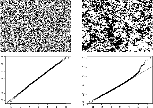
Figure 1: Two-dimensional excursion sets and normal Q–Q plots of their areas. The columns correspond to short-range and long-range dependent models (from left to right).

In example Figure 1 the first row shows two-dimensional excursion sets for realizations of two types of random fields (from left to right): short-range dependent normal scale mixture model and long-range dependent Cauchy model, consults Section 9. The excursion sets are shown in black colour. The Q–Q plots in the second row, which correspond to the models shown above, suggest that the limit law of the short-range dependent model is normal, while for the long-range dependent model the data are not normally distributed. Additional details about Figure 1 are provided in Section 9.

The paper has three aims. One is to provide explicit, albeit asymptotic, formulae for the distribution of the volume of excursion sets of a class of strongly dependent random fields. The second one is to derive asymptotic results for heavy-tailed random fields. Finally, the third aim is to generalize the previous findings to sojourn measures above moving levels and for cross-correlated scenarios.

There is, therefore, a need for models that are able to display strongly dependent heavy-tailed behaviour and yet are sufficiently simple to allow analysis. To obtain explicit results we detail the underlying structure of random fields. Namely, a basic assumption of the analysis is that we examine functionals of vector Gaussian random fields, in particular, Student and Fisher–Snedecor random fields. Consult [3, 15, 16, 47] on excursion sets of chi-square, Student and Fisher–Snedecor random fields and their importance for image analysis and studies of brain function. Other results on sojourn measures of chi-square random fields can be found in [23, 29, 30, 27].

Minkowski functionals are widely used to characterise geometric properties of random fields, in particular in the analysis of cosmic microwave background radiation, see [36, 38]. In this paper we investigate the first Minkowski functional of random fields and its expansions into multidimensional Hermite polynomials, see some one-dimensional/discrete counterparts in [18, 20]. To have a complete account of results on asymptotic distributions of sojourn measures for functions of vector random fields, we also prove corresponding theorems for weakly dependent scenarios.

The remainder of the paper is structured as follows. In Sections 2–4, we introduce the necessary background from the theory of random fields and briefly review some definitions and notation on the first Minkowski functional, multidimensional Hermite expansions, and Student and Fisher–Snedecor random fields. We start Sections 5 and 7 with generalizations and corrections of some classical asymptotic results to arbitrary sets and vector fields. With this in hand, we continue Sections 5 and 7 by new results for the first Minkowski functional of Student and Fisher–Snedecor random fields. In Section 7, we also show how to lift these results to sojourn measures above moving levels and for cross-correlated underlying vector fields. Sections 6 and 8 provide the proofs of all theorems and lemmata in the article. Simulation results on the limit distributions of areas of excursion sets for two types of images are given in Section 9. Short conclusions are made in Section 10.

In this paper, we only consider real-valued random fields. $|\cdot|$ and $\|\cdot\|$ denote the Lebesgue measure and the distance in $\mathbb{R}^{d}$, respectively. In what follows, we use the symbol $C$ to denote constants which are not important for our discussion. Moreover, the same symbol $C$ may be used for different constants appearing in the same proof.

2 First Minkowski functional

In this section, we review the definition of the first Minkowski functional and its relevant properties. More information about stochastic Minkowski functionals and their links with the expected Euler characteristics of excursion sets can be found in [2].

We consider a measurable mean square continuous homogeneous isotropic random field $S(x),x\in\mathbb{R}^{d}$, (see [23, 27]) with $\mathbf{E}S(x)=m$, and the covariance function

$$\mathrm{B}(r):=\operatorname{\mathbf{Cov}}\bigl{(}S(x),S(y)\bigr{)}=\int_{0}^{\infty}Y_{d}(rz)\,\mathrm{d}\Phi(z),\qquad x,y\in\mathbb{R}^{d},$$

where $r:=\|x-y\|$, $\Phi(\cdot)$ is the isotropic spectral measure, $Y_{d}(\cdot)$ is the spherical Bessel function given by

$$Y_{1}(z) := \cos z,$$

$$Y_{n}(z) := 2^{(n-2)/2}\Gamma\biggl{(}\frac{n}{2}\biggr{)}J_{(n-2)/2}(z)z^{(2-n)/2},\qquad z\geq 0,n\geq 2,$$

$J_{\nu}(\cdot)$ is the Bessel function of the first kind of order $\nu>-1/2$.

We define the marginal c.d.f. $H(\cdot)$ and p.d.f. $h(\cdot)$ of the field $S(x)$ as follows:

$$H(u)=\mathbf{P}\bigl{\{}S(x)\leq u\bigr{\}},\qquad H(u)=\int_{-\infty}^{u}h(z)\,\mathrm{d}z,\qquad u\in\mathbb{R}.$$

Definition 1.

$S(x)$, $x\in\mathbb{R}^{d}$, is a homogeneous isotropic random field possessing an absolutely continuous spectrum, if there exists a function $f(\cdot)$ such that

$$\Phi(z)=2\uppi^{d/2}\Gamma^{-1}(d/2)\int_{0}^{z}u^{d-1}f(u)\,\mathrm{d}u,\qquad u^{d-1}f(u)\in\mathbf{L}_{1}(\mathbb{R}_{+}).$$

The function $f(\cdot)$ is called the isotropic spectral density function of the field $S(x)$.

Consider a Jordan-measurable convex bounded set $\Delta\subset\mathbb{R}^{d}$, such that $|\Delta|>0$ and $\Delta$ contains the origin in its interior. Let $\Delta(r),r>0$, be the homothetic image of the set $\Delta$, with the centre of homothety in the origin and the coefficient $r>0$, that is, $|\Delta(r)|=r^{d}|\Delta|$.

Definition 2.

The first Minkowski functional is defined as

$$M_{r}\{S\}:=\bigl{|}\bigl{\{}x\in\Delta(r)\colon\ S(x)>a(r)\bigr{\}}\bigr{|}=\int_{\Delta(r)}\chi\bigl{(}S(x)>a(r)\bigr{)}\,\mathrm{d}x,$$

where $\chi(\cdot)$ is an indicator function and $a(r)$ is a continuous non-decreasing function.

In the simplest case $a(r)=a$ is a constant. The functional $M_{r}\{S\}$ has an interpretation of the sojourn measure of the random field $S(x)$ above the constant level $a$, or the moving level $a(r)$.

For the first Minkowski functional $M_{r}\{S\}$ we obtain:

$$\mathbf{E}M_{r}\{S\}=|\Delta|r^{d}\mathbf{P}\bigl{\{}S(x)>a(r)\bigr{\}}=|\Delta|r^{d}\bigl{(}1-H\bigl{(}a(r)\bigr{)}\bigr{)}$$ (1)

and

$$\operatorname{\mathbf{Var}}M_{r}\{S\}=\int_{\Delta(r)}\int_{\Delta(r)}\mathbf{P}\bigl{\{}S(x)>a(r),S(y)>a(r)\bigr{\}}\,\mathrm{d}x\,\mathrm{d}y-\bigl{[}\mathbf{E}M_{r}\{S\}\bigr{]}^{2},$$

or

$$\operatorname{\mathbf{Var}}M_{r}\{S\}=\int_{\Delta(r)}\int_{\Delta(r)}\operatorname{\mathbf{Cov}}\bigl{(}\zeta(x),\zeta(y)\bigr{)}\,\mathrm{d}x\,\mathrm{d}y,$$

where $\zeta(x):=\chi(S(x)>a(r))$, $x\in\mathbb{R}^{d}$. Therefore, it is important to investigate the integrals

$$\int_{\Delta(r)}\int_{\Delta(r)}G\bigl{(}\|x-y\|\bigr{)}\,\mathrm{d}x\,\mathrm{d}y$$

of various integrable Borel functions $G(\cdot)$.

Consider the uniform distribution on $\Delta(r)$ with the p.d.f. given by

$$q_{\Delta(r)}(x)=\cases{\displaystyle\frac{1}{r^{d}|\Delta|},&\quad$\mbox{if }x\in\Delta(r)$;\vspace*{2pt}\cr 0,&\quad$\mbox{if }x\notin\Delta(r).$}$$

Let $U$ and $V$ be two independent and uniformly distributed inside the set $\Delta(r)$ random vectors. We denote by $\psi_{\Delta(r)}(\rho)$, $\rho\geq 0$, the p.d.f. of the distance $\|U-V\|$ between $U$ and $V$. Note that $\psi_{\Delta(r)}(\rho)=0$ if $\rho>\mathrm{diam}\{\Delta(r)\}$. Using the above notation, we obtain the representation

$$\int_{\Delta(r)}\int_{\Delta(r)}G\bigl{(}\|x-y\|\bigr{)}\,\mathrm{d}x\,\mathrm{d}y = |\Delta|^{2}r^{2d}\mathbf{E}G\bigl{(}\|U-V\|\bigr{)}$$

$$= |\Delta|^{2}r^{2d}\int_{0}^{\mathrm{diam}\{\Delta(r)\}}G(\rho)\psi_{\Delta(r)}(\rho)\,\mathrm{d}\rho.$$

Example 1.

If $\Delta(r)$ is the ball $v(r):=\{x\in\mathbb{R}^{d}\colon\ \|x\|<r\}$ then

$$\psi_{v(r)}(\rho)=d\rho^{d-1}r^{-d}I_{1-(\rho/2r)^{2}}\biggl{(}\frac{d+1}{2},\frac{1}{2}\biggr{)},\qquad 0\leq\rho\leq 2r,$$

where

$$I_{\mu}(p,q):=\frac{\Gamma(p+q)}{\Gamma(p)\Gamma(q)}\int_{0}^{\mu}t^{p-1}(1-t)^{q-1}\,\mathrm{d}t,\qquad\mu\in(0,1],p>0,q>0,$$ (3)

is the incomplete beta function, see [23].

Several expressions for $\psi_{v(r)}(\rho)$, $0\leq\rho\leq 2r$, are given below:

1. [$d=1$:]

2. $\psi_{v(r)}(\rho)=\frac{1}{r}(1-\frac{\rho}{2r})$,

3. $\psi_{v(r)}(\rho)=\frac{4\rho}{\uppi r^{2}}(\arccos\frac{\rho}{2r}-\frac{\rho}{2r}\sqrt{1-(\frac{\rho}{2r})^{2}})$,

4. $\psi_{v(r)}(\rho)=\frac{3\rho^{2}}{r^{3}}(1-\frac{\rho}{2r})^{2}(1+\frac{\rho}{4r})$.

If one considers the functional

$$F_{r}(\zeta)=\int_{v(r)}\zeta(x)\,\mathrm{d}x,$$

then

$$\operatorname{\mathbf{Var}}F_{r}(\zeta) = \int_{v(r)}\int_{v(r)}\tilde{\mathrm{B}}\bigl{(}\|x-y\|\bigr{)}\,\mathrm{d}x\,\mathrm{d}y=\bigl{|}v(1)\bigr{|}^{2}r^{2d}\mathbf{E}\tilde{\mathrm{B}}\bigl{(}\|U-V\|\bigr{)}$$

$$= \frac{4\uppi^{d}}{d\Gamma^{2}(d/2)}r^{d}\int_{0}^{2r}z^{d-1}\tilde{\mathrm{B}}(z)I_{1-({z}/{2r})^{2}}\biggl{(}\frac{d+1}{2},\frac{1}{2}\biggr{)}\,\mathrm{d}z,$$

where $\tilde{\mathrm{B}}(\cdot)$ is a covariance function of $\zeta(x)$.

For some random fields these formulae can be specified, however the asymptotic analysis is difficult. Therefore, we will use an approach based on multidimensional Hermite expansions.

3 Multidimensional Hermite expansions

Let $H_{k}(u)$, $k\geq 0$, $u\in\mathbb{R}$, be the Hermite polynomials, see [41].

Lemma 1

[41] Let $(\xi_{1},\ldots,\xi_{2p})$ be $2p$-dimensional zero mean Gaussian vector with

$$\mathbf{E}\xi_{j}\xi_{k}=\cases{1,&\quad$\mbox{if }k=j$;\vspace*{2pt}\cr r_{j},&\quad$\mbox{if }k=j+p\mbox{ and }1\leq j\leq p;$\vspace*{2pt}\cr 0,&\quad$\mbox{otherwise.}$}$$

Then

$$\mathbf{E}\prod_{j=1}^{p}H_{k_{j}}(\xi_{j})H_{m_{j}}(\xi_{j+p})=\prod_{j=1}^{p}\delta_{k_{j}}^{m_{j}}k_{j}!r_{j}^{k_{j}}.$$

Let us denote

$$e_{\nu}(w):=\prod_{j=1}^{p}H_{k_{j}}(w_{j}),$$

where $w=(w_{1},\ldots,w_{p})^{\prime}\in\mathbb{R}^{p}$, $\nu=(k_{1},\ldots,k_{p})\in\mathbb{Z}^{p}$, and all $k_{j}\geq 0$ for $j=1,\ldots,p$.

The summation theorem for Hermite polynomials [21], formula (8.958.1) states that

$$H_{k}\biggl{(}\frac{\sum_{j=1}^{p}a_{j}w_{j}}{\sum_{j=1}^{p}a^{2}_{j}}\biggr{)}=\frac{k!}{(\sum_{j=1}^{p}a^{2}_{j})^{k/2}}\sum_{k_{1}+\cdots+k_{p}=k}\prod_{j=1}^{p}\frac{a_{j}^{k_{j}}}{k_{j}!}H_{k_{j}}(w_{j}).$$ (4)

The polynomials $\{e_{\nu}(w)\}_{\nu}$ form a complete orthogonal system in the Hilbert space

$$\mathbf{L}_{2}\bigl{(}\mathbb{R}^{p},\phi\bigl{(}\|w\|\bigr{)}\,\mathrm{d}w\bigr{)} = \biggl{\{}G\colon\ \int_{\mathbb{R}^{p}}G^{2}(w)\phi\bigl{(}\|w\|\bigr{)}\,\mathrm{d}w<\infty\biggr{\}},$$

$$\phi\bigl{(}\|w\|\bigr{)} = \prod_{j=1}^{p}\phi(w_{j}),\qquad\phi(w_{j})=\frac{1}{\sqrt{2\uppi}}\mathrm{e}^{-{w_{j}^{2}}/{2}}.$$

An arbitrary function $G(w)\in\mathbf{L}_{2}(\mathbb{R}^{p},\phi(\|w\|)\,\mathrm{d}w)$ admits the mean-square convergent expansion

$$G(w)=\sum_{k=0}^{\infty}\sum_{\nu\in N_{k}}\frac{C_{\nu}e_{\nu}(w)}{\nu!},\qquad C_{\nu}:=\int_{\mathbb{R}^{p}}G(w)e_{\nu}(w)\phi\bigl{(}\|w\|\bigr{)}\,\mathrm{d}w,$$ (5)

where $N_{k}:=\{(k_{1},\ldots,k_{p})\in\mathbb{Z}^{p}\colon\ \sum_{j=1}^{p}k_{j}=k,\mbox{ all }k_{j}\geq 0\mbox{ for }j=1,\ldots,p\},$ $\nu!:=k_{1}!\cdots k_{p}!$

By Parseval’s identity

$$\sum_{k=0}^{\infty}\sum_{\nu\in N_{k}}\frac{C_{\nu}^{2}}{\nu!}=\int_{R^{p}}G^{2}(w)\phi\bigl{(}\|w\|\bigr{)}\,\mathrm{d}w.$$ (6)

Definition 3.

Let $G(w)\in\mathbf{L}_{2}(\mathbb{R}^{p},\phi(\|w\|)\,\mathrm{d}w)$ and there exist an integer $\kappa\geq 1$ such that $C_{\nu}=0$, for all $\nu\in N_{k}$, $0\leq k\leq\kappa-1$, but $C_{\nu}\neq 0$ for at least one tuple $\nu=(k_{1},\ldots,k_{p})\in N_{\kappa}$. Then $\kappa$ is called the Hermite rank of $G(\cdot)$ and denoted by $H\operatorname{rank}G$.

Let $\eta(x)=[\eta_{1}(x),\ldots,\eta_{p}(x)]^{\prime}$, $x\in\mathbb{R}^{d}$, be a measurable mean-square continuous homogeneous isotropic vector Gaussian random field, see Section 5 in [27], Section 1.2. Suppose that the components $\eta_{1}(\cdot),\ldots,\eta_{p}(\cdot)$ are independent, $\mathbf{E}\eta_{j}(0)=0$, $\mathbf{E}\eta_{j}^{2}(0)=1$, and $\mathbf{E}\eta_{j}(0)\eta_{j}(x)=\mathrm{B}_{jj}(\|x\|)$, $1\leq j\leq p$.

If $G(w)\in\mathbf{L}_{2}(\mathbb{R}^{p},\phi(\|w\|)\,\mathrm{d}w)$ then the integral functional $F(\eta)=\int_{\Delta(r)}G(\eta(x))\,\mathrm{d}x$ can be represented as

$$F(\eta)=\sum_{k=0}^{\infty}\sum_{\nu\in N_{k}}\frac{C_{\nu}}{\nu!}\int_{\Delta(r)}e_{\nu}\bigl{(}\eta(x)\bigr{)}\,\mathrm{d}x.$$

Therefore the expectation of $F(\eta)$ is

$$\mathbf{E}F(\eta)=\bigl{|}\Delta(r)\bigr{|}C_{(0,\ldots,0)},$$ (7)

while by Lemma 1 the variance is equal

$$\operatorname{\mathbf{Var}}F(\eta)=\sum_{k=0}^{\infty}\sum_{\nu\in N_{k}}\frac{C_{\nu}^{2}}{\nu!}\int_{\Delta(r)}\int_{\Delta(r)}\prod_{j=1}^{p}\mathrm{B}_{jj}^{k_{j}}\bigl{(}\|x-y\|\bigr{)}\,\mathrm{d}x\,\mathrm{d}y.$$ (8)

4 Student and Fisher–Snedecor random fields

In this section, we introduce two main models investigated in the paper, namely, Student and Fisher–Snedecor random fields proposed for studies of brain function in [47].

Let us consider the vector random field

$$\eta(x)=\bigl{[}\eta_{1}(x),\ldots,\eta_{m}(x),\eta_{m+1}(x),\ldots,\eta_{m+n}(x)\bigr{]}^{\prime},$$

which consists of $n+m$ independent copies of a measurable mean-square continuous homogeneous isotropic zero-mean and unit variance Gaussian random field $\eta_{1}(x)$, $x\in\mathbb{R}^{d}$.

Definition 4.

The Fisher–Snedecor random field $F_{m,n}(x)$, $x\in\mathbb{R}^{d}$, is defined by

$$F_{m,n}(x):=\frac{({1}/{m})(\eta_{1}^{2}(x)+\cdots+\eta_{m}^{2}(x))}{({1}/{n})(\eta_{m+1}^{2}(x)+\cdots+\eta_{m+n}^{2}(x))},\qquad x\in\mathbb{R}^{d}.$$

The random field $F_{m,n}(x)$, $x\in\mathbb{R}^{d},$ has the marginal Fisher–Snedecor distribution with the p.d.f.

$$h(u)=\frac{m^{{m}/{2}}n^{{n}/{2}}\Gamma({(m+n)}/{2})}{\Gamma({m}/{2})\Gamma({n}/{2})}\cdot\frac{u^{{m}/{2}-1}}{(n+mu)^{{(n+m)}/{2}}},\qquad u\in[0,\infty),$$

and the c.d.f.

$$H(u)=I_{{mu}/{(n+mu)}}\biggl{(}\frac{m}{2},\frac{n}{2}\biggr{)}.$$ (9)

By properties of the Fisher–Snedecor distribution

$$\mathbf{E}\bigl{[}F_{m,n}(x)\bigr{]}^{r}=\frac{\Gamma({(m+2k)}/{2})\Gamma({(n-2k)}/{2})}{\Gamma({m}/{2})\Gamma({n}/{2})}\biggl{(}\frac{n}{m}\biggr{)}^{r},\qquad n>2r.$$

Definition 5.

The Student random field $T_{n}(x)$, $x\in\mathbb{R}^{d}$, is defined by

$$T_{n}(x):=\frac{\eta_{1}(x)}{\sqrt{({1}/{n})(\eta_{2}^{2}(x)+\cdots+\eta_{n+1}^{2}(x))}},\qquad x\in\mathbb{R}^{d}.$$

It has the marginal Student $t_{n}$-distribution with the p.d.f.

$$h(u)=\frac{\Gamma({(n+1)}/{2})}{\sqrt{n\uppi}\Gamma({n}/{2})}\cdot\biggl{(}1+\frac{u^{2}}{n}\biggr{)}^{-{(n+1)}/{2}},\qquad u\in\mathbb{R},$$

and the c.d.f.

$$H(u)=\frac{1}{2}+\frac{1}{2}\biggl{(}1-I_{{n}/{(n+u^{2})}}\biggl{(}\frac{n}{2},\frac{1}{2}\biggr{)}\biggr{)}\cdot\operatorname{sgn}(u),$$ (10)

where $\operatorname{sgn}(\cdot)$ is the signum function.

The $r$th moments of $T_{n}(x)$ exist when $n>r$ and for $k\in\mathbb{N}$ we have

$$\mathbf{E}\bigl{\{}T_{n}(x)\bigr{\}}^{r}=\cases{0,&\quad$\mbox{if }r=2k-1<n$;\vspace*{2pt}\cr\displaystyle\frac{\Gamma({(r+1)}/{2})\Gamma({(n-r)}/{2})n^{r/2}}{\sqrt{\uppi}\Gamma({n}/{2})},&\quad$\mbox{if }r=2k<n$.}$$

Note that $[T_{n}(x)]^{2}=F_{1,n}(x),x\in\mathbb{R}^{d}$.

Remark 0.

The right-hand tail of the p.d.f. of the $F_{m,n}$-distribution decreases as $x^{-{(n+2)}/{2}}$. The left and the right-hand tails of the p.d.f. of the $t$-distribution decrease as $|x|^{-n-1}$. Thus, both Student and Fisher–Snedecor random fields have heavy-tailed marginal distributions.

5 Central limit theorem for functionals of weakly dependent vector random fields

In this section we present some analogues of results in [4, 5, 13, 22] for the case of integrals of weakly dependent vector random fields. Then, we apply these results to Fisher–Snedecor and Student random fields.

Let $\eta(x)=[\eta_{1}(x),\ldots,\eta_{p}(x)]^{\prime}$, $x\in\mathbb{R}^{d}$, be a measurable mean-square continuous homogeneous isotropic vector Gaussian random field with $\mathbf{E}\eta(x)=0$ and covariance matrix

$$\mathbf{B}\bigl{(}\|x\|\bigr{)}=\mathbf{E}\eta(0)\eta(x)^{\prime}=\bigl{(}\mathrm{B}_{ij}\bigl{(}\|x\|\bigr{)}\bigr{)}_{1\leq i,j\leq p}.$$

First, we need an auxiliary statement which is similar to Theorem 1 in [13]. Let $\Box_{u,v}(r):=\{x\in\mathbb{R}^{d}\colon\ ru_{i}<x_{i}\leq rv_{i},i=1,\ldots,d\}$, where $u,v\in\mathbb{R}^{d}$ and $u_{i}<v_{i}$ for all $1\leq i\leq d$. We will use the notation

$$\psi(x):=\max_{1\leq i\leq p}\sum_{j=1}^{p}\bigl{|}\mathrm{B}_{ij}\bigl{(}\|x\|\bigr{)}\bigr{|}.$$

Lemma 2

Suppose that the function $G(\cdot)$ has Hermite rank $\kappa\geq 1$, the covariance matrix of the vector field $\eta(x)$ satisfies the conditions $\psi(\cdot)\in\mathbf{L}_{\kappa}(\mathbb{R}^{d})$ and $\psi(x)\leq 1$ for all $x\in\mathbb{R}^{d}$, and

$$\sigma^{2}:=\int_{\mathbb{R}^{d}}\mathbf{E}\bigl{[}G\bigl{(}\eta(0)\bigr{)}G\bigl{(}\eta(x)\bigr{)}\bigr{]}\,\mathrm{d}x\neq 0.$$

Then

$$r^{-d/2}\int_{\Box_{u,v}(r)}G\bigl{(}\eta(x)\bigr{)}\,\mathrm{d}x\stackrel{{\scriptstyle\mathcal{D}}}{{\to}}Y_{\Box_{u,v}},\qquad r\to\infty,$$

where $|\Box_{u,v}(1)|^{-1/2}Y_{\Box_{u,v}}\sim N(0,\sigma^{2})$, $|\Box_{u,v}(1)|=\prod_{i=1}^{d}(v_{i}-u_{i})$.

If $\Box_{u^{(1)},v^{(1)}}(1)\cap\Box_{u^{(2)},v^{(2)}}(1)=\varnothing$, $u^{(i)},v^{(i)}\in\mathbb{R}^{d}$, $i=1,2$, then the random variables $Y_{\Box_{u^{(1)},v^{(1)}}}$ and $Y_{\Box_{u^{(2)},v^{(2)}}}$ are independent.

The proof of the lemma is based on Lemma 1, the diagram formula and ideas in [13], see also [4, 5] for vector processes, and the application of the diagram technique for random fields in [23]. The assumption $\psi(\cdot)\in\mathbf{L}_{\kappa}(\mathbb{R}^{d})$ can be weakened, consult, for example, the conditions (1.4^′) and (1.4^′′) in Theorem 1^′ [13]. The most recent results can be found in [7, 24, 39, 41].

The following result generalizes Theorem 4 in [4] to the case of integrals of weakly dependent vector random fields.

Theorem 1

If the conditions of Lemma 2 are satisfied, then

$$r^{-d/2}\int_{\Delta(r)}G\bigl{(}\eta(x)\bigr{)}\,\mathrm{d}x\stackrel{{\scriptstyle\mathcal{D}}}{{\to}}Y_{\Delta},\qquad r\to\infty,$$

where $|\Delta|^{-1/2}Y_{\Delta}\sim N(0,\sigma^{2})$.

Remark 0.

The central limit theorems for the volumes of excursion sets of stationary quasi-associated random fields were proved in [14, 37]. The approach used in the papers did not require the isotropy of Gaussian fields. However, it was assumed that the continuous covariance function is ${\mathcal{O}}(\|x\|^{-\alpha})$, $\alpha>d$, when $\|x\|\to\infty$. We obtain the central limit theorems for homogeneous isotropic random fields but under different conditions. Namely, it follows from (11) that only the integrability of the covariance functions is required.

In the next two theorems we consider sojourn measures of Fisher–Snedecor and Student random fields above the constant level $a(r)\equiv a$. In the notation of Sections 2 and 4, for the Fisher–Snedecor random field $p=m+n$ and the first Minkowski functional takes the form

$$M_{r}\{F_{m,n}\}=\bigl{|}\bigl{\{}x\in\Delta(r)\colon\ F_{m,n}(x)>a\bigr{\}}\bigr{|}=\int_{\Delta(r)}\chi\bigl{(}F_{m,n}(x)>a\bigr{)}\,\mathrm{d}x.$$

Theorem 2

If the covariance matrix of the Fisher–Snedecor random field $F_{m,n}(x)$, $x\in\mathbb{R}^{d}$, satisfies the two conditions: $\sup_{x\in R^{d}}\psi(x)\leq 1$ and $\psi(\cdot)\in\mathbf{L}_{2}({\mathbb{R}^{d}})$, then

$$r^{-d/2}M_{r}\{F_{m,n}\}-|\Delta|r^{d/2}\biggl{(}1-I_{{ma}/{(n+ma)}}\biggl{(}\frac{m}{2},\frac{n}{2}\biggr{)}\biggr{)}\stackrel{{\scriptstyle\mathcal{D}}}{{\to}}Y_{\Delta},\qquad r\to\infty,$$

where $|\Delta|^{-1/2}Y_{\Delta}\sim N(0,\sigma_{F}^{2}(a))$, $I_{\mu}(p,q)$ is defined by (3),

$$\sigma_{F}^{2}(a):=\int_{\mathbb{R}^{d}}\mathbf{E}\bigl{[}\chi\bigl{(}F_{m,n}(0)>a\bigr{)}\chi\bigl{(}F_{m,n}(x)>a\bigr{)}\bigr{]}\,\mathrm{d}x.$$

For the Student, random field $p=n+1$ and the first Minkowski functional for the constant level $a$ is

$$M_{r}\{T_{n}\}=\bigl{|}\bigl{\{}x\in\Delta(r)\colon\ T_{n}(x)>a\bigr{\}}\bigr{|}=\int_{\Delta(r)}\chi\bigl{(}T_{n}(x)>a\bigr{)}\,\mathrm{d}x.$$

Theorem 3

If the covariance matrix of the Student random field $T_{n}(x)$, $x\in\mathbb{R}^{d}$, satisfies the two conditions: $\sup_{x\in R^{d}}\psi(x)\leq 1$ and $\psi(\cdot)\in\mathbf{L}_{1}({\mathbb{R}^{d}})$, then

$$r^{-d/2}M_{r}\{T_{n}\}-|\Delta|r^{d/2}\biggl{(}\frac{1}{2}-\frac{1}{2}\biggl{(}1-I_{{n}/{(n+a^{2})}}\biggl{(}\frac{n}{2},\frac{1}{2}\biggr{)}\biggr{)}\cdot\operatorname{sgn}(a)\biggr{)}\stackrel{{\scriptstyle\mathcal{D}}}{{\to}}\tilde{Y}_{\Delta},\qquad r\to\infty,$$

where $|\Delta|^{-1/2}\tilde{Y}_{\Delta}\sim N(0,\sigma_{T}^{2})$,

$$\sigma_{T}^{2}:=\int_{\mathbb{R}^{d}}\mathbf{E}\bigl{[}\chi\bigl{(}T_{n}(0)>a\bigr{)}\chi\bigl{(}T_{n}(x)>a\bigr{)}\bigr{]}\,\mathrm{d}x.$$

6 Proofs of the results of Section 5

Proof of Lemma 2 The lemma can be proved by a modification of the proof of Theorem 1 [13] using vector results in [4, 5]. To avoid lengthy repetitions, we only state required changes to Theorem 1 [13].

The first step is the replacement of the function of a single variable $H(t)$ in Theorem 1 by the function of multiple variables $G(x)$ and use vector notation and conditions on the covariance matrix presented in [5]. Then, it is straightforward to replace the summation over the sets $B(n,N):=\{s=(s_{1},\ldots,s_{d})\in\mathbb{Z}^{d}\colon\ Nn_{i}<s_{i}\leq N(n_{i}+1),i=1,\ldots,d\}$, by the integration over the multidimensional parallelepipeds $\Box_{u,v}(r):=\{x\in\mathbb{R}^{d}\colon\ ru_{i}<x_{i}\leq rv_{i},i=1,\ldots,d\}$. Finally, using integrals instead of sums in Theorem 4 [4] we obtain $\lim_{r\to\infty}r^{-d}\operatorname{\mathbf{Var}}(\int_{\Box_{u,v}(r)}G(\eta(x))\,\mathrm{d}x)$ and the expression for $\sigma^{2}$.

The condition $\psi(\cdot)\in\mathbf{L}_{\kappa}(\mathbb{R}^{d})$ guarantees that cross-correlation functions of all components of $\eta(x)$ are also in $\mathbf{L}_{\kappa}(\mathbb{R}^{d})$.

Proof of Theorem 1 Let us consider a coverage of $\Delta(r)$ by the finite union $\Box_{J}(r):=\bigcup_{j\in J}\Box_{u^{(j)},v^{(j)}}(r)$ of the disjoint multidimensional parallelepipeds $\{\Box_{u^{(j)},v^{(j)}}(r),j\in J\}$, with the following properties:

1. $\Box_{J}(r)$ is a decreasing nested sequence of sets when $r$ is fixed and $|J|\to\infty$;

2. $\Delta\subset\Box_{J}(1)$;

3. $|\Box_{J}(1)\setminus\Delta|\to 0$, when $|J|\to\infty$.

The existence of such $\Box_{J}(1)$ follows form the fact that $\Delta$ is a Jordan-measurable set.

By Lemma 2, we obtain

$$r^{-d/2}\int_{\Box_{J}(r)}G\bigl{(}\eta(x)\bigr{)}\,\mathrm{d}x\stackrel{{\scriptstyle\mathcal{D}}}{{\to}}Y_{\Box_{J}},\qquad r\to\infty,$$

where $|\Box_{J}(1)|^{-1/2}Y_{\Box_{J}}\sim N(0,\sigma^{2})$.

By the properties of $\Box_{J}(r)$, we get $Y_{\Box_{J}}\stackrel{{\scriptstyle\mathcal{D}}}{{\to}}Y_{\Delta},|J|\to\infty$.

As $\psi(x)\leq 1$, then by Lemma 1 [4]

$$\bigl{|}\mathbf{E}\bigl{[}G\bigl{(}\eta(x)\bigr{)}G\bigl{(}\eta\bigl{(}x^{(1)}\bigr{)}\bigr{)}\bigr{]}\bigr{|}\leq\psi^{\kappa}\bigl{(}\bigl{\|}x-x^{(1)}\bigr{\|}\bigr{)}\mathbf{E}G^{2}\bigl{(}\eta(0)\bigr{)},\qquad x,x^{(1)}\in\mathbb{R}^{d}.$$ (11)

It follows from inequality (11) that

$$r^{-d}\operatorname{\mathbf{Var}}\biggl{(}\int_{\Box_{J}(r)}G\bigl{(}\eta(x)\bigr{)}\,\mathrm{d}x-\int_{\Delta(r)}G\bigl{(}\eta(x)\bigr{)}\,\mathrm{d}x\biggr{)}$$

$$\quad=r^{-d}\int_{\Box_{J}(r)\setminus\Delta(r)}\int_{\Box_{J}(r)\setminus\Delta(r)}\mathbf{E}G\bigl{(}\eta(x)\bigr{)}G\bigl{(}\eta\bigl{(}x^{(1)}\bigr{)}\bigr{)}\,\mathrm{d}x\,\mathrm{d}x^{(1)}$$

(12)

$$\quad\leq\frac{\mathbf{E}G^{2}(\eta(0))}{r^{d}}\int_{\Box_{J}(r)\setminus\Delta(r)}\int_{\Box_{J}(r)\setminus\Delta(r)}\psi^{\kappa}\bigl{(}\bigl{\|}x-x^{(1)}\bigr{\|}\bigr{)}\,\mathrm{d}x\,\mathrm{d}x^{(1)}$$

$$\quad\leq\bigl{|}\Box_{J}(1)\setminus\Delta\bigr{|}\cdot\mathbf{E}G^{2}\bigl{(}\eta(0)\bigr{)}\int_{\mathbb{R}^{d}}\psi^{\kappa}\bigl{(}\|x\|\bigr{)}\,\mathrm{d}x.$$

Finally, by property 3 of $\Box_{J}(r)$ the upper bound in (6) approaches 0 when $|J|\to\infty$, which completes the proof.

Proof of Theorem 2 Note that by (9)

$$\mathbf{E}\bigl{(}\chi\bigl{(}F_{m,n}(x)>a\bigr{)}\bigr{)}=\mathbf{P}\bigl{(}F_{m,n}(x)>a\bigr{)}=1-I_{{ma}/{(n+ma)}}\biggl{(}\frac{m}{2},\frac{n}{2}\biggr{)}.$$

Then it follows from (1) that

$$\mathbf{E}\biggl{(}r^{-d/2}\int_{\Delta(r)}\chi\bigl{(}F_{m,n}(x)>a\bigr{)}\,\mathrm{d}x\biggr{)}=|\Delta|r^{d/2}\biggl{(}1-I_{{ma}/{(n+ma)}}\biggl{(}\frac{m}{2},\frac{n}{2}\biggr{)}\biggr{)}$$

and we obtain the following representation

$$r^{-d/2}\int_{\Delta(r)}\bigl{(}\chi\bigl{(}F_{m,n}(x)>a\bigr{)}-\mathbf{E}\bigl{(}\chi\bigl{(}F_{m,n}(x)>a\bigr{)}\bigr{)}\bigr{)}\,\mathrm{d}x=r^{-d/2}\int_{\Delta(r)}G\bigl{(}\eta(x)\bigr{)}\,\mathrm{d}x,$$

where

$$G(w)=\chi\biggl{(}\frac{({1}/{m})(w_{1}^{2}+\cdots+w_{m}^{2})}{({1}/{n})(w_{m+1}^{2}+\cdots+w_{m+n}^{2})}>a\biggr{)}+I_{{ma}/{(n+ma)}}\biggl{(}\frac{m}{2},\frac{n}{2}\biggr{)}-1.$$ (13)

$G(\cdot)$ is a symmetric function with respect to the origin. Hence, $C_{\nu}=0$ for all $\nu\in N_{1}$. However, $C_{\nu}\neq 0$ for such tuples $\nu=(k_{1},\ldots,k_{m+n})\in N_{2}$ that exactly one $k_{i}=2$ (expressions for coefficients $C_{\nu}$, $\nu\in N_{2}$, will be given in Theorem 7).

Therefore, $H\operatorname{rank}G=2$ and we can apply Theorem 1 which completes the proof.

Proof of Theorem 3 It is easy to obtain the statement of the theorem following steps analogous to the proof of Theorem 2.

Using (10), we conclude that

$$\mathbf{E}\bigl{(}\chi\bigl{(}T_{n}(x)>a\bigr{)}\bigr{)}=\frac{1}{2}-\frac{1}{2}\biggl{(}1-I_{{n}/{(n+a^{2})}}\biggl{(}\frac{n}{2},\frac{1}{2}\biggr{)}\biggr{)}\cdot\operatorname{sgn}(a).$$

Therefore,

$$r^{-d/2}\int_{\Delta(r)}\bigl{(}\chi\bigl{(}T_{n}(x)>a\bigr{)}-\mathbf{E}\bigl{(}\chi\bigl{(}T_{n}(x)>a\bigr{)}\bigr{)}\bigr{)}\,\mathrm{d}x=r^{-d/2}\int_{\Delta(r)}\tilde{G}\bigl{(}\xi(x)\bigr{)}\,\mathrm{d}x,$$

where

$$\tilde{G}(w)=\chi\biggl{(}\frac{w_{1}}{\sqrt{({1}/{n})(w_{2}^{2}+\cdots+w_{n+1}^{2})}}>a\biggr{)}+\frac{1}{2}\biggl{(}1-I_{{n}/{(n+a^{2})}}\biggl{(}\frac{n}{2},\frac{1}{2}\biggr{)}\biggr{)}\cdot\operatorname{sgn}(a)-\frac{1}{2}.$$ (14)

For $\tilde{G}(\cdot)$ the coefficient $C_{(1,0,\ldots,0)}\neq 0$, $(1,0,\ldots,0)\in N_{1}$, (expressions for coefficients $C_{\nu}$, $\nu\in N_{1}$, will be given in Theorem 6). Therefore, $H\operatorname{rank}\tilde{G}=1$ and the application of Theorem 1 completes the proof.

7 Non-central limit theorem for functionals of strongly dependent vector random fields

In this section, we first present corrections and generalizations to arbitrary sets of some results for random fields in [23], Section 2.10, [27], Sections 2.4 and 3.4, and [31]. Consult also the pioneering papers [19, 44, 45] and the book [9] on non-central limit theorems and the Hermite polynomials approach. In the rest of this section, we apply the developed technique to Fisher–Snedecor and Student random fields.

Assumption 1.

Let $\eta(x)=[\eta_{1}(x),\ldots,\eta_{p}(x)]^{\prime}$, $x\in\mathbb{R}^{d}$, be a vector homogeneous isotropic Gaussian random field with $\mathbf{E}\eta(x)=0$ and covariance matrix

$$\mathbf{\tilde{B}}(0)=\mathcal{I},\qquad\mathbf{\tilde{B}}\bigl{(}\|x\|\bigr{)}=\mathbf{E}\eta(0)\eta(x)^{\prime}=\mathcal{I}\cdot\|x\|^{-\alpha}L\bigl{(}\|x\|\bigr{)},\qquad\alpha>0,$$

where $\mathcal{I}$ is the unit matrix of size $p$, $L(\|\cdot\|)$ is a function slowly varying at infinity.

We investigate the random variables

$$K_{r}:=\int_{\Delta(r)}G_{r}\bigl{(}\eta(x)\bigr{)}\,\mathrm{d}x\quad\mbox{and}\quad K_{r,\kappa}:=\sum_{\nu\in N_{\kappa}}\frac{C_{\nu}(r)}{\nu!}\int_{\Delta(r)}e_{\nu}\bigl{(}\eta(x)\bigr{)}\,\mathrm{d}x,$$

where $C_{\nu}(r)$ are coefficients of the Hermite series (5) of the function $G_{r}(\cdot)$ for fixed $r$.

Theorem 4

Suppose that $\eta(x)$ satisfies Assumption 1 for $\alpha\in(0,d/\kappa)$, for each sufficiently large $r$ $H\operatorname{rank}G_{r}(\cdot)=\kappa\geq 1$, and

$$\biggl{(}\sum_{\nu\in N_{\kappa}}\frac{C_{\nu}^{2}(r)}{\nu!}\biggr{)}^{-1}\sum_{l\geq\kappa+1}\sum_{\nu\in N_{l}}\frac{C_{\nu}^{2}(r)}{\nu!}=\mathrm{o}\bigl{(}r^{\gamma/2}\bigr{)},\qquad r\to\infty,$$ (15)

where $\gamma\in(0,\min(\alpha,d-\alpha\kappa))$.

If there exists the limit distribution for at least one of the random variables

$$\frac{K_{r}}{\sqrt{\operatorname{\mathbf{Var}}K_{r}}}\quad\mbox{and}\quad\frac{K_{r,\kappa}}{\sqrt{\operatorname{\mathbf{Var}}K_{r,\kappa}}},$$

then the limit distribution of the other random variable exists too and the limit distributions coincide when $r\to\infty$.

Remark 0.

If $G_{r}(w)\in\mathbf{L}_{2}(R^{p},\phi(\|w\|)\,\mathrm{d}w)$ does not depend on $r$ and has Hermitian rank $\kappa$, then (15) is satisfied.

Remark 0.

In many cases it is much easier to compute $\operatorname{\mathbf{Var}}K_{r,\kappa}$ than $\operatorname{\mathbf{Var}}K_{r}$. Using the property $\lim_{r\to\infty}{\operatorname{\mathbf{Var}}K_{r}}/{\operatorname{\mathbf{Var}}K_{r,\kappa}}=1,$ we can change the statement of Theorem 4 as follows: under the assumptions of Theorem 4 limit distributions of the random variables ${K_{r}}/{\sqrt{\operatorname{\mathbf{Var}}K_{r,\kappa}}}$ and ${K_{r,\kappa}}/{\sqrt{\operatorname{\mathbf{Var}}K_{r,\kappa}}}$ coincide when $r\to\infty$.

Assumption 2.

$\eta_{1}(x)$ has a spectral density $f(\|\lambda\|)$, $\lambda\in\mathbb{R}^{d}$, such that

$$f\bigl{(}\|\lambda\|\bigr{)}\sim c_{2}(d,\alpha)\|\lambda\|^{\alpha-d}L\biggl{(}\frac{1}{\|\lambda\|}\biggr{)},\qquad\|\lambda\|\to 0,$$ (16)

where $0<\alpha<d$ and

$$c_{2}(d,\alpha):=\frac{\Gamma({(d-\alpha)}/2)}{2^{\alpha}\uppi^{d/2}\Gamma(\alpha/2)}.$$

Remark 0.

If $f(\cdot)$ is decreasing in a neighbourhood of zero and continuous for all $\lambda\neq 0$, then by Tauberian Theorem 4 [28] the statement $\mathrm{B}(\|x\|)=\mathbf{E}\eta_{1}(0)\eta_{1}(x)=\|x\|^{-\alpha}L(\|x\|)$ implies Assumption 2. A much more detailed discussion of relations between Assumption 1 and 2 can be found in [28, 40].

Note that then the field possesses the spectral representation

$$\eta_{1}(x)=\int_{\mathbb{R}^{d}}\mathrm{e}^{\mathrm{i}\langle\lambda,x\rangle}\sqrt{f\bigl{(}\|\lambda\|\bigr{)}}W(\mathrm{d}\lambda),$$

where $W(\cdot)$ is the complex Gaussian white noise random measure on $\mathbb{R}^{d}$.

Let

$$\mathcal{K}(x):=\int_{\Delta}\mathrm{e}^{\mathrm{i}\langle x,u\rangle}\,\mathrm{d}u,\qquad x\in\mathbb{R}^{d}.$$ (17)

Theorem 5

Let $\eta_{1}(x)$, $x\in\mathbb{R}^{d}$, be a homogeneous isotropic Gaussian random field with $\mathbf{E}\eta_{1}(x)=0$. If Assumptions 1 and 2 hold, $\alpha\in(0,d/\kappa)$, and $\kappa\geq 1$, then for $r\to\infty$ the finite-dimensional distributions of

$$X_{\kappa,r}:=r^{(\kappa\alpha)/2-d}L^{-\kappa/2}(r)\int_{\Delta(r)}H_{\kappa}\bigl{(}\eta_{1}(x)\bigr{)}\,\mathrm{d}x$$

converge weakly to the finite-dimensional distributions of

$$X_{\kappa}:=c_{2}^{\kappa/2}(d,\alpha)\int_{\mathbb{R}^{d\kappa}}^{{\prime}}\mathcal{K}(\lambda_{1}+\cdots+\lambda_{\kappa})\frac{W(\mathrm{d}\lambda_{1})\cdots W(\mathrm{d}\lambda_{\kappa})}{\|\lambda_{1}\|^{(d-\alpha)/2}\cdots\|\lambda_{\kappa}\|^{(d-\alpha)/2}},$$ (18)

where $\int_{R^{d\kappa}}^{{\prime}}$ denotes the multiple Wiener–Itô integral.

The following result shows that $X_{\kappa}$ is correctly defined and ${\mathbf{E}}X_{\kappa}^{2}<\infty$.

Lemma 3

If $\tau_{1},\ldots,\tau_{\kappa}$, $\kappa\geq 1$, are such positive constants, that $\sum_{i=1}^{\kappa}\tau_{i}<d$, then

$$\int_{\mathbb{R}^{d\kappa}}\bigl{|}\mathcal{K}(\lambda_{1}+\cdots+\lambda_{\kappa})\bigr{|}^{2}\frac{\mathrm{d}\lambda_{1}\cdots\mathrm{d}\lambda_{\kappa}}{\|\lambda_{1}\|^{d-\tau_{1}}\cdots\|\lambda_{\kappa}\|^{d-\tau_{\kappa}}}<\infty.$$ (19)

If $\tau_{1}=\cdots=\tau_{\kappa}=\alpha$, $\alpha\in(0,d/\kappa)$, then we will use the following notation

$$c_{3}(\kappa,d,\alpha):=\int_{\mathbb{R}^{d\kappa}}\bigl{|}\mathcal{K}(\lambda_{1}+\cdots+\lambda_{\kappa})\bigr{|}^{2}\frac{\mathrm{d}\lambda_{1}\cdots\mathrm{d}\lambda_{\kappa}}{\|\lambda_{1}\|^{d-\alpha}\cdots\|\lambda_{\kappa}\|^{d-\alpha}}.$$

Remark 0.

It is not difficult to adapt Theorem 5 for the case of stochastic processes and obtain self-similar limit processes, consults [23, 27, 31, 37]. For $\kappa=2$, the limit random variable $X_{2}$ in Theorem 5 plays an analogous role to the Rosenblatt distribution, see [44].

Example 2.

If $\Delta$ is the ball $v(1)$, then

$$\mathcal{K}(x)=\int_{v(1)}\mathrm{e}^{\mathrm{i}\langle x,u\rangle}\,\mathrm{d}u=(2\uppi)^{d/2}\frac{J_{d/2}(\|x\|)}{\|x\|^{d/2}},\qquad x\in\mathbb{R}^{d},$$

and we obtain the result from [23], Section 2.10, with $t=1$, that is,

$$X_{\kappa}=(2\uppi)^{d/2}c_{2}^{\kappa/2}(d,\alpha)\int_{\mathbb{R}^{d\kappa}}^{{\prime}}\frac{J_{d/2}(\|\lambda_{1}+\cdots+\lambda_{\kappa}\|)}{\|\lambda_{1}+\cdots+\lambda_{\kappa}\|^{d/2}}\frac{W(\mathrm{d}\lambda_{1})\cdots W(\mathrm{d}\lambda_{\kappa})}{\|\lambda_{1}\|^{(d-\alpha)/2}\cdots\|\lambda_{\kappa}\|^{(d-\alpha)/2}}.$$

Example 3.

Let us consider $\eta(x)$ with uncorrelated identically distributed components possessing covariance functions of the form

$$B_{jj}\bigl{(}\|x\|\bigr{)}=\bigl{(}1+\|x\|^{{}\sigma}\bigr{)}^{-\theta},\qquad\sigma\in(0,2],\theta>0,j=1,\ldots,p.$$

The above is known as the generalized Linnik covariance function. Cauchy field in the simulation results of Section 9 is an important particular case of this model.

If $\sigma\theta\kappa>d$, $\kappa\geq 1$, then $\eta(x)$ is a weakly dependent random field which satisfies the assumptions of Section 5, that is, $\psi(x)=B_{11}(\|x\|)\in\mathbf{L}_{\kappa}(\mathbb{R}^{d})$ and $\psi(x)\leq 1$ for all $x\in\mathbb{R}^{d}$. If $\sigma\theta<d$, then we have the strongly dependent case and Assumptions 1 and 2 hold, see [28] and references therein.

In the next two theorems, we apply the general results to study the sojourn measure of strongly dependent Fisher–Snedecor and Student random fields above a constant level, that is, $a(r)\equiv a$. The following theorem demonstrates that for Student random fields, even in the case of strong dependence, we have a normal limit law. However, for the strongly dependent case the normalization is different from $r^{-d/2}$ in Theorem 3.

Theorem 6

Let $\eta(x)=[\eta_{1}(x),\ldots,\eta_{n+1}(x)]^{\prime}$, $x\in\mathbb{R}^{d}$, satisfy Assumption 1 for $\alpha\in(0,d)$, and Assumption 2 hold for the spectral density of each component $\eta_{j}(\cdot)$. Then the random variable

$$U_{r}(n,\alpha):=\sqrt{2\uppi}\bigl{(}1+a^{2}/n\bigr{)}^{n/2}\frac{M_{r}\{T_{n}\}-|\Delta|r^{d}(1/2-1/2(1-I_{{n}/{(n+a^{2})}}({n}/{2},{1}/{2}))\cdot\operatorname{sgn}(a))}{r^{d-\alpha/2}L^{1/2}(r)\sqrt{c_{2}(d,\alpha)c_{3}(1,d,\alpha)}}$$

is asymptotically $\mathcal{N}(0,1)$, as $r\to\infty$.

Contrary to the Student case, for strongly dependent Fisher–Snedecor random fields we obtain a non-normal limit law.

Theorem 7

Let $\eta(x)=[\eta_{1}(x),\ldots,\eta_{n+m}(x)]^{\prime}$, $x\in\mathbb{R}^{d}$, satisfy Assumption 1 for $\alpha\in(0,d/2)$, and Assumption 2 hold for the spectral density of each component $\eta_{j}(\cdot)$. Then, for $r\to\infty$, the distribution of the random variable

$$U_{r}(m,n,\alpha):=\frac{M_{r}\{F_{m,n}\}-|\Delta|r^{d}(1-I_{{ma}/{(n+ma)}}({m}/{2},{n}/{2}))}{c_{4}(a,n,m)r^{d-\alpha}L(r)}$$

converges to the distribution of the random variable

$$R(m,n):=\frac{X_{2,1}+\cdots+X_{2,m}}{m}-\frac{X_{2,m+1}+\cdots+X_{2,m+n}}{n},$$

where $X_{2,j}$, $j=1,\ldots,m+n$, are independent copies of the random variable $X_{2}$ defined by (18),

$$c_{4}(a,n,m):=\frac{(ma/n)^{m/2}\Gamma((m+n)/2)}{(1+ma/n)^{(m+n)/2}\Gamma(n/2)\Gamma(m/2)}.$$

Now we generalize the previous results to the increasing level $a(r)\to+\infty$, as $r\to+\infty$.

Theorem 8

Let $\eta(x)=[\eta_{1}(x),\ldots,\eta_{n+1}(x)]^{\prime}$, $x\in\mathbb{R}^{d}$, satisfy Assumption 1 for $\alpha\in(0,d)$, and Assumption 2 hold for the spectral density of each component $\eta_{j}(\cdot)$. If $a(r)=\mathrm{o}(r^{\gamma/2n})$, $\gamma\in(0,\min(\alpha,d-\alpha))$, $r\to\infty$, then the random variable

$$\sqrt{2\uppi}\bigl{(}1+a(r)^{2}/n\bigr{)}^{n/2}\frac{M_{r}\{T_{n}\}-|\Delta|r^{d}I_{{n}/{(n+a^{2}(r))}}({n}/{2},{1}/{2})}{r^{d-\alpha/2}L^{1/2}(r)\sqrt{c_{2}(d,\alpha)c_{3}(1,d,\alpha)}}$$

is asymptotically $\mathcal{N}(0,1)$.

Theorem 9

Let $\eta(x)=[\eta_{1}(x),\ldots,\eta_{n+m}(x)]^{\prime}$, $x\in\mathbb{R}^{d}$, satisfy Assumption 1 for $\alpha\in(0,d/2)$, and Assumption 2 hold for the spectral density of each component $\eta_{j}(\cdot)$. If $a(r)=\mathrm{o}(r^{\gamma/n})$, $\gamma\in(0,\min(\alpha,d-\alpha))$, $r\to\infty$, then the distribution of the random variable

$$\frac{M_{r}\{F_{m,n}\}-|\Delta|r^{d}(1-I_{{ma(r)}/{(n+ma(r))}}({m}/{2},{n}/{2}))}{c_{4}(a(r),n,m)r^{d-\alpha}L(r)}$$

converges to the distribution of the random variable $R(m,n)$ defined in Theorem 7.

The following theorems illustrate how to extend the obtained results to long range dependent vector fields which components may be cross-correlated, consult the pioneering papers [34, 35, 46] on similar vector Gaussian process results. Such cross-correlated random fields may be useful in positron emission tomography studies to identify brain activated regions. In many cases, the activation is so small that the experiment must be repeated several times and the scan results are averaged to improve the signal-to-noise ratio. The cross-correlated components $\eta_{j}(x)$, $j=1,\ldots,p$, can be interpreted as repeated imaged slices in scans of the same subject. If the stationarity assumption is in doubt, Student and Fisher–Snedecor random fields were proposed to test regional changes, consult [15, 47].

We use the previous notation $M_{r}\{T_{n}\}$ and $M_{r}\{F_{m,n}\}$, but replace independent components of $\eta(\cdot)$ in the definitions 4 and 5 by components of cross-correlated random fields. Note, that the functional $M_{r}\{T_{n}\}$ ($M_{r}\{F_{m,n}\}$) takes the same value on the class of fields $\{C\eta(x),C>0\}$. Therefore, we study only the cases where $\det(\mathbf{E}\eta(0)\eta(0)^{\prime})=1$.

Assumption 3.

Let $\eta(x)=[\eta_{1}(x),\ldots,\eta_{p}(x)]^{\prime}$, $x\in\mathbb{R}^{d}$, be a vector homogeneous isotropic zero mean Gaussian random field such that

$$\mathbf{B}\bigl{(}\|x\|\bigr{)}=\mathbf{E}\eta(0)\eta(x)^{\prime}=\mathcal{A}\cdot\|x\|^{-\alpha}L\bigl{(}\|x\|\bigr{)},\qquad\alpha\in(0,d/\kappa),\kappa\geq 1,$$

where $\mathcal{A}$ is a $p\times p$ positive-semidefinite symmetric orthogonal matrix, and Assumption 2 hold for the spectral density of each component of the field $\tilde{\eta}:=\mathcal{A}^{-1/2}\eta$.

Note that, by the definition of $\mathcal{A}$, there exists the square root of $\mathcal{A}^{-1}$, that is, the positive-semidefinite orthogonal matrix $\mathcal{A}^{-1/2}$, such that $\mathcal{A}^{-1/2}\mathcal{A}^{-1/2}=\mathcal{A}^{-1}$. In what follows, we denote $\mathcal{A}^{-1/2}:=(a_{ij})_{1\leq i,j\leq p}$.

Theorem 10

If $\eta(x)=[\eta_{1}(x),\ldots,\eta_{n+1}(x)]^{\prime}$, $x\in\mathbb{R}^{d}$, satisfies Assumption 3 for $\kappa=1$, then $U_{r}(n,\alpha)$ defined in Theorem 6 is asymptotically $\mathcal{N}(0,1)$, as $r\to\infty$.

For the Fisher–Snedecor random field, we only consider the case of a block diagonal matrix $\mathcal{A}$. It is also possible to derive similar results for arbitrary $\mathcal{A}$, but for such cases we need a generalization of Theorem 5 about the asymptotic behaviour of the bivariate functionals $\int_{\Delta(r)}\eta_{j}(x)\eta_{l}(x)\,\mathrm{d}x$ (consult [46] for $d=1$), which is beyond the scope of this paper.

Theorem 11

Let $\eta(x)=[\eta_{1}(x),\ldots,\eta_{n+m}(x)]^{\prime}$, $x\in\mathbb{R}^{d}$, satisfy Assumption 3 for $\kappa=2$ and $\mathcal{A}=\bigl{[}{\mathcal{A}_{1}\atop 0}\enskip{0\atop\mathcal{A}_{2}}\bigr{]}$, where $\mathcal{A}_{1}$ and $\mathcal{A}_{2}$ are $m\times m$ and $n\times n$ matrices, respectively. Then, for $r\to\infty$, the distribution of the random variable $U_{r}(m,n,\alpha)$ converges to the distribution of the random variable $R(m,n)$, where $U_{r}(m,n,\alpha)$ and $R(m,n)$ are defined in Theorem 7.

8 Proofs of the results of Section 7

Proof of Theorem 4Let

$$V_{r}:=\sum_{l\geq\kappa+1}\sum_{\nu\in N_{l}}\frac{C_{\nu}(r)}{\nu!}\int_{\Delta(r)}e_{\nu}\bigl{(}\eta(x)\bigr{)}\,\mathrm{d}x,$$

then by Lemma 1

$$\operatorname{\mathbf{Var}}K_{r}=\operatorname{\mathbf{Var}}K_{r,\kappa}+\operatorname{\mathbf{Var}}V_{r}.$$

By (8) and (2)

$$\operatorname{\mathbf{Var}}K_{r,\kappa} = \sum_{\nu\in N_{\kappa}}\frac{C_{\nu}^{2}(r)}{\nu!}\int_{\Delta(r)}\int_{\Delta(r)}\|x-y\|^{-\alpha\kappa}L^{\kappa}\bigl{(}\|x-y\|\bigr{)}\,\mathrm{d}x\,\mathrm{d}y$$

$$= |\Delta|^{2}r^{2d-\alpha\kappa}\sum_{\nu\in N_{\kappa}}\frac{C_{\nu}^{2}(r)}{\nu!}\int_{0}^{\mathrm{diam}\{\Delta\}}z^{-\alpha\kappa}L^{\kappa}(rz)\psi_{\Delta}(z)\,\mathrm{d}z.$$

If $\alpha\in(0,d/\kappa)$, then by asymptotic properties of integrals of slowly varying functions (see Theorem 2.7 [43]) we get

$$\operatorname{\mathbf{Var}}K_{r,\kappa} = c_{1}(\kappa,\alpha,\Delta)|\Delta|^{2}\sum_{\nu\in N_{\kappa}}\frac{C_{\nu}^{2}(r)}{\nu!}r^{2d-\kappa\alpha}L^{\kappa}(r)\bigl{(}1+\mathrm{o}(1)\bigr{)},\qquad r\to\infty,$$

where

$$c_{1}(\kappa,\alpha,\Delta):=\int_{0}^{\mathrm{diam}\{\Delta\}}z^{-\alpha\kappa}\psi_{\Delta}(z)\,\mathrm{d}z.$$

Similar to $\operatorname{\mathbf{Var}}K_{r,\kappa}$ we obtain

$$\operatorname{\mathbf{Var}}V_{r}=|\Delta|^{2}r^{2d}\sum_{l\geq\kappa+1}\sum_{\nu\in N_{l}}\frac{C_{\nu}^{2}(r)}{\nu!}\int_{0}^{r\cdot\mathrm{diam}\{\Delta\}}z^{-\alpha l}L^{l}(z)\psi_{\Delta(r)}(z)\,\mathrm{d}z.$$

It follows from $z^{-\alpha}L(z)\in[0,1]$, $z\geq 0$, that

$$\operatorname{\mathbf{Var}}V_{r} \leq |\Delta|^{2}r^{2d-(\kappa+1)\alpha}\sum_{l\geq\kappa+1}\sum_{\nu\in N_{l}}\frac{C_{\nu}^{2}(r)}{\nu!}\int_{0}^{\mathrm{diam}\{\Delta\}}z^{-\alpha(\kappa+1)}L^{\kappa+1}(rz)\psi_{\Delta}(z)\,\mathrm{d}z$$

$$= |\Delta|^{2}r^{2d-\kappa\alpha}L^{\kappa}(r)\sum_{l\geq\kappa+1}\sum_{\nu\in N_{l}}\frac{C_{\nu}^{2}(r)}{\nu!}\int_{0}^{\mathrm{diam}\{\Delta\}}z^{-\alpha\kappa}\frac{L^{\kappa}(rz)}{L^{\kappa}(r)}\frac{L(rz)}{(rz)^{\alpha}}\psi_{\Delta}(z)\,\mathrm{d}z.$$

Let us split the above integral into two parts $I_{1}$ and $I_{2}$ with the ranges of integration $[0,r^{-\beta}]$ and $(r^{-\beta},\mathrm{diam}\{\Delta\}]$, respectively, where $\beta\in(0,1)$.

As $z^{-\alpha}L(z)\in[0,1]$, $z\geq 0$, we can estimate the first integral as follows

$$I_{1} \leq \int_{0}^{r^{-\beta}}z^{-\alpha\kappa}\frac{L^{\kappa}(rz)}{L^{\kappa}(r)}\psi_{\Delta}(z)\,\mathrm{d}z\leq\frac{\sup_{0\leq s\leq r^{1-\beta}}s^{\delta}L^{\kappa}(s)}{r^{\delta}L^{\kappa}(r)}\int_{0}^{r^{-\beta}}z^{-\delta}z^{-\alpha\kappa}\psi_{\Delta}(z)\,\mathrm{d}z$$

$$\leq \biggl{(}\frac{\sup_{0\leq s\leq r}s^{\delta/k}L(s)}{r^{\delta/k}L(r)}\biggr{)}^{\kappa}\int_{0}^{r^{-\beta}}z^{-\delta}z^{-\alpha\kappa}\psi_{\Delta}(z)\,\mathrm{d}z.$$

By Theorem 1.5.3 [10] and the definition of slowly varying functions

$$\lim_{r\to\infty}\frac{\sup_{0\leq s\leq r}s^{\delta/k}L(s)}{r^{\delta/k}L(r)}=1.$$

By (2), we can estimate the integral in (8) as follows

$$\int_{0}^{r^{-\beta}}z^{-\delta}z^{-\alpha\kappa}\psi_{\Delta}(z)\,\mathrm{d}z = |\Delta|^{-2}\int_{\Delta}\int_{\Delta}\chi\bigl{(}\|x-y\|\leq r^{-\beta}\bigr{)}\|x-y\|^{-(\delta+\alpha\kappa)}\,\mathrm{d}x\,\mathrm{d}y$$

$$\leq |\Delta|^{-1}\int_{0}^{r^{-\beta}}\rho^{d-(1+\delta+\alpha\kappa)}\,\mathrm{d}\rho=\frac{r^{-\beta(d-(\delta+\alpha\kappa))}}{(d-(\delta+\alpha\kappa))|\Delta|}.$$

For the second integral, we obtain

$$I_{2}\leq\frac{\sup_{r^{1-\beta}\leq s\leq r\cdot\mathrm{diam}\{\Delta\}}s^{\delta}L^{\kappa}(s)}{r^{\delta}L^{\kappa}(r)}\cdot\sup_{r^{1-\beta}\leq s\leq r\cdot\mathrm{diam}\{\Delta\}}\frac{L(s)}{s^{\alpha}}\cdot\int_{0}^{\mathrm{diam}\{\Delta\}}z^{-(\delta+\alpha\kappa)}\psi_{\Delta}(z)\,\mathrm{d}z.$$

Using Theorem 1.5.3 [10], we conclude that

$$\lim_{r\to\infty}\frac{\sup_{r^{1-\beta}\leq s\leq r\cdot\mathrm{diam}\{\Delta\}}s^{\delta}L^{\kappa}(s)}{r^{\delta}L^{\kappa}(r)} \leq \lim_{r\to\infty}\frac{\sup_{0\leq s\leq r\cdot\mathrm{diam}\{\Delta\}}s^{\delta}L^{\kappa}(s)}{(r\cdot\mathrm{diam}\{\Delta\})^{\delta}L^{\kappa}(r\cdot\mathrm{diam}\{\Delta\})}$$

$${}\times\lim_{r\to\infty}\frac{\mathrm{diam}^{\delta}\{\Delta\}L^{\kappa}(r\cdot\mathrm{diam}\{\Delta\})}{L^{\kappa}(r)}=\mathrm{diam}^{\delta}\{\Delta\}.$$

By Proposition 1.3.6 and Theorem 1.5.3 [10], it follows that

$$\sup_{r^{1-\beta}\leq s\leq r\cdot\mathrm{diam}\{\Delta\}}\frac{L(s)}{s^{\alpha}}\leq\frac{\sup_{s\geq r^{1-\beta}}s^{-\alpha}L(s)}{r^{-\alpha(1-\beta)}L(r^{1-\beta})}\cdot\frac{L(r^{1-\beta})}{r^{\delta(1-\beta)}}\cdot r^{(\delta-\alpha)(1-\beta)}=\mathrm{o}\bigl{(}r^{(\delta-\alpha)(1-\beta)}\bigr{)}.$$ (22)

We can choose $\beta=1/2$ and make $\delta$ arbitrary close to 0. Then by (8), (22), and condition (15) we obtain

$$\lim_{r\to\infty}\frac{\operatorname{\mathbf{Var}}V_{r}}{\operatorname{\mathbf{Var}}K_{r}}=0\quad\mbox{and}\quad\lim_{r\to\infty}\frac{\operatorname{\mathbf{Var}}K_{r}}{\operatorname{\mathbf{Var}}K_{r,\kappa}}=1.$$

Thus,

$$\lim_{r\to\infty}\mathbf{E}\biggl{(}\frac{K_{r}}{\sqrt{\operatorname{\mathbf{Var}}K_{r}}}-\frac{K_{r,\kappa}}{\sqrt{\operatorname{\mathbf{Var}}K_{r,\kappa}}}\biggr{)}^{2}=\lim_{r\to\infty}\frac{\mathbf{E}(V_{r}+(1-\sqrt{{\operatorname{\mathbf{Var}}K_{r}}/{\operatorname{\mathbf{Var}}K_{r,\kappa}}})K_{r,\kappa})^{2}}{\operatorname{\mathbf{Var}}K_{r}}=0,$$

which completes the proof.

Proof of Lemma 3 Definition (17) yields $\mathcal{K}(\cdot)\in\mathbf{L}_{\infty}(\mathbb{R}^{d})$ and by the Plancherel theorem $\mathcal{K}(\cdot)\in\mathbf{L}_{2}(\mathbb{R}^{d})$. Hence, the statement of the lemma is valid for $\kappa=1$. For $\kappa>1$, we can obtain (19) by the recursive estimation routine and the change of variables $\tilde{\lambda}_{\kappa-1}={\lambda_{\kappa-1}}/{\|u\|}$:

$$\int_{\mathbb{R}^{d\kappa}}\bigl{|}\mathcal{K}(\lambda_{1}+\cdots+\lambda_{\kappa})\bigr{|}^{2}\frac{\mathrm{d}\lambda_{1}\cdots\mathrm{d}\lambda_{\kappa}}{\|\lambda_{1}\|^{d-\tau_{1}}\cdots\|\lambda_{\kappa}\|^{d-\tau_{\kappa}}}$$

$$\quad=\int_{\mathbb{R}^{d(\kappa-1)}}\bigl{|}\mathcal{K}(\lambda_{1}+\cdots+\lambda_{\kappa-2}+u)\bigr{|}^{2}$$

$$\qquad{}\times\int_{\mathbb{R}^{d}}\frac{d\lambda_{\kappa-1}}{\|\lambda_{\kappa-1}\|^{d-\tau_{\kappa-1}}\|u-\lambda_{\kappa-1}\|^{d-\tau_{\kappa}}}\cdot\frac{\mathrm{d}\lambda_{1}\cdots\mathrm{d}\lambda_{\kappa-2}\,\mathrm{d}u}{\|\lambda_{1}\|^{d-\tau_{1}}\cdots\|\lambda_{\kappa-2}\|^{d-\tau_{\kappa-2}}}$$

$$\quad=\int_{\mathbb{R}^{d(\kappa-1)}}\frac{|\mathcal{K}(\lambda_{1}+\cdots+\lambda_{\kappa-2}+u)|^{2}\,\mathrm{d}\lambda_{1}\cdots\mathrm{d}\lambda_{\kappa-2}}{\|\lambda_{1}\|^{d-\tau_{1}}\cdots\|\lambda_{\kappa-2}\|^{d-\tau_{\kappa-2}}\|u\|^{d-\tau_{\kappa-1}-\tau_{\kappa}}}$$

$$\qquad{}\times\int_{\mathbb{R}^{d}}\frac{\mathrm{d}\tilde{\lambda}_{\kappa-1}}{\|\tilde{\lambda}_{\kappa-1}\|^{d-\tau_{\kappa-1}}\|{u}/{\|u\|}-\tilde{\lambda}_{\kappa-1}\|^{d-\tau_{\kappa}}}\,\mathrm{d}u$$

$$\quad\leq C\int_{\mathbb{R}^{d(\kappa-1)}}\bigl{|}\mathcal{K}(\lambda_{1}+\cdots+\lambda_{\kappa-2}+u)\bigr{|}^{2}\frac{\mathrm{d}\lambda_{1}\cdots\mathrm{d}\lambda_{\kappa-2}\,\mathrm{d}u}{\|\lambda_{1}\|^{d-\tau_{1}}\cdots\|\lambda_{\kappa-2}\|^{d-\tau_{\kappa-2}}\|u\|^{d-\tau_{\kappa-1}-\tau_{\kappa}}}$$

$$\quad\leq\cdots$$

$$\quad\leq C\int_{\mathbb{R}^{d}}\bigl{|}\mathcal{K}(u)\bigr{|}^{2}\frac{\mathrm{d}u}{\|u\|^{d-\sum_{i=1}^{\kappa}\tau_{i}}}<\infty.$$

Proof of Theorem 5 Using the self-similarity of Gaussian white noise, namely $W(C\,\mathrm{d}\lambda)\stackrel{{\scriptstyle\mathcal{D}}}{{=}}C^{d/2}W(\mathrm{d}\lambda)$, and the Itó formula [19]

$$H_{\kappa}\bigl{(}\eta_{1}(x)\bigr{)}=\int_{\mathbb{R}^{d\kappa}}^{\prime}\mathrm{e}^{\mathrm{i}\langle\lambda_{1}+\cdots+\lambda_{\kappa},x\rangle}\Biggl{\{}\prod_{j=1}^{\kappa}\sqrt{f(\lambda_{j})}\Biggr{\}}W(\mathrm{d}\lambda_{1})\cdots W(\mathrm{d}\lambda_{\kappa})$$

we obtain

$$X_{\kappa,r}\stackrel{{\scriptstyle\mathcal{D}}}{{=}}c_{2}^{\kappa/2}(d,\alpha)\int_{\mathbb{R}^{d\kappa}}^{{\prime}}\mathcal{K}(\lambda_{1}+\cdots+\lambda_{\kappa})Q_{r}(\lambda_{1},\ldots,\lambda_{\kappa})\frac{W(\mathrm{d}\lambda_{1})\cdots W(\mathrm{d}\lambda_{\kappa})}{\|\lambda_{1}\|^{(d-\alpha)/2}\cdots\|\lambda_{\kappa}\|^{(d-\alpha)/2}},$$

where

$$Q_{r}(\lambda_{1},\ldots,\lambda_{\kappa}):=r^{\kappa(\alpha-d)/2}L^{-\kappa/2}(r)c_{2}^{-\kappa/2}(d,\alpha)\Biggl{[}\prod_{j=1}^{\kappa}\|\lambda_{j}\|^{d-\alpha}f\biggl{(}\frac{\|\lambda_{j}\|}{r}\biggr{)}\Biggr{]}^{1/2}.$$

By the isometry property of multiple stochastic integrals

$$R_{r}:=\frac{\mathbb{E}|X_{\kappa,r}-X_{\kappa}|^{2}}{c_{2}^{\kappa}(d,\alpha)}=\int_{\mathbb{R}^{d\kappa}}\frac{|\mathcal{K}(\lambda_{1}+\cdots+\lambda_{\kappa})|^{2}(Q_{r}(\lambda_{1},\ldots,\lambda_{\kappa})-1)^{2}}{\|\lambda_{1}\|^{d-\alpha}\cdots\|\lambda_{\kappa}\|^{d-\alpha}}\,\mathrm{d}\lambda_{1}\cdots\mathrm{d}\lambda_{\kappa}.$$

Using (16) and properties of slowly varying functions we conclude that $Q_{r}(\lambda_{1},\ldots,\lambda_{\kappa})$ converges pointwise to 1, when $r\to\infty$. Hence, by Lebesgue’s dominated convergence theorem the integral converges to zero if there is some integrable function which dominates integrands for all $r$.

Let us split $\mathbb{R}^{d\kappa}$ into the regions

$$B_{\mu}:=\bigl{\{}(\lambda_{1},\ldots,\lambda_{\kappa})\in\mathbb{R}^{d\kappa}\colon\ \|\lambda_{j}\|\leq 1,\mbox{ if }\mu_{j}=-1,\mbox{ and }\|\lambda_{j}\|>1,\mbox{ if }\mu_{j}=1,j=1,\ldots,\kappa\bigr{\}},$$

where $\mu=(\mu_{1},\ldots,\mu_{\kappa})\in\{-1,1\}^{\kappa}$ is a binary vector of length $\kappa$. Then we can represent the integral $R_{r}$ as

$$R_{r}:=\bigcup_{\mu\in\{-1,1\}^{\kappa}}\int_{B_{\mu}}\bigl{|}\mathcal{K}(\lambda_{1}+\cdots+\lambda_{\kappa})\bigr{|}^{2}\bigl{(}Q_{r}(\lambda_{1},\ldots,\lambda_{\kappa})-1\bigr{)}^{2}\frac{\mathrm{d}\lambda_{1}\cdots\mathrm{d}\lambda_{\kappa}}{\|\lambda_{1}\|^{d-\alpha}\cdots\|\lambda_{\kappa}\|^{d-\alpha}}.$$

If $(\lambda_{1},\ldots,\lambda_{\kappa})\in B_{\mu}$ we estimate the integrand as follows

$$\frac{|\mathcal{K}(\lambda_{1}+\cdots+\lambda_{\kappa})|^{2}(Q_{r}(\lambda_{1},\ldots,\lambda_{\kappa})-1)^{2}}{\|\lambda_{1}\|^{d-\alpha}\cdots\|\lambda_{\kappa}\|^{d-\alpha}}$$

$$\quad\leq\frac{2|\mathcal{K}(\lambda_{1}+\cdots+\lambda_{\kappa})|^{2}}{\|\lambda_{1}\|^{d-\alpha}\cdots\|\lambda_{\kappa}\|^{d-\alpha}}\bigl{(}Q^{2}_{r}(\lambda_{1},\ldots,\lambda_{\kappa})+1\bigr{)}$$

$$\quad=\frac{2|\mathcal{K}(\lambda_{1}+\cdots+\lambda_{\kappa})|^{2}}{\|\lambda_{1}\|^{d-\alpha}\cdots\|\lambda_{\kappa}\|^{d-\alpha}}\Biggl{(}\prod_{j=1}^{\kappa}\|\lambda_{j}\|^{\mu_{j}\delta}\cdot\prod_{j=1}^{\kappa}\frac{({r}/{\|\lambda_{j}\|})^{\mu_{j}\delta}L({r}/{\|\lambda_{j}\|})}{r^{\mu_{j}\delta}L(r)}+1\Biggr{)}$$

$$\quad\leq\frac{2|\mathcal{K}(\lambda_{1}+\cdots+\lambda_{\kappa})|^{2}}{\|\lambda_{1}\|^{d-\alpha}\cdots\|\lambda_{\kappa}\|^{d-\alpha}}\Biggl{(}1+\prod_{j=1}^{\kappa}\|\lambda_{1}\|^{\mu_{j}\delta}\cdot\sup_{(\lambda_{1},\ldots,\lambda_{\kappa})\in B_{\mu}}\prod_{j=1}^{\kappa}\frac{({r}/{\|\lambda_{j}\|})^{\mu_{j}\delta}L({r}/{\|\lambda_{j}\|})}{r^{\mu_{j}\delta}L(r)}\Biggr{)},$$

where $\delta$ is an arbitrary positive number. By Theorem 1.5.3 [10]

$$\lim_{r\to\infty}\frac{\sup_{\|\lambda_{j}\|\leq 1}({r}/{\|\lambda_{j}\|})^{-\delta}L({r}/{\|\lambda_{j}\|})}{r^{-\delta}L(r)} = \lim_{r\to\infty}\frac{\sup_{z\geq r}z^{-\delta}L(z)}{r^{-\delta}L(r)}=1;$$

$$\lim_{r\to\infty}\frac{\sup_{\|\lambda_{j}\|>1}({r}/{\|\lambda_{j}\|})^{\delta}L({r}/{\|\lambda_{j}\|})}{r^{\delta}L(r)} = \lim_{r\to\infty}\frac{\sup_{z\in[0,r]}z^{\delta}L(z)}{r^{\delta}L(r)}=1.$$

Therefore, there exists $r_{0}>0$ such that for all $r\geq r_{0}$ and $(\lambda_{1},\ldots,\lambda_{\kappa})\in B_{\mu}$

$$\frac{|\mathcal{K}(\lambda_{1}+\cdots+\lambda_{\kappa})|^{2}(Q_{r}(\lambda_{1},\ldots,\lambda_{\kappa})-1)^{2}}{\|\lambda_{1}\|^{d-\alpha}\cdots\|\lambda_{\kappa}\|^{d-\alpha}}$$

$$\quad\leq\frac{2|\mathcal{K}(\lambda_{1}+\cdots+\lambda_{\kappa})|^{2}}{\|\lambda_{1}\|^{d-\alpha}\cdots\|\lambda_{\kappa}\|^{d-\alpha}}$$ (23)

$$\qquad{}+2C\frac{|\mathcal{K}(\lambda_{1}+\cdots+\lambda_{\kappa})|^{2}}{\|\lambda_{1}\|^{d-\alpha-\mu_{1}\delta}\cdots\|\lambda_{\kappa}\|^{d-\alpha-\mu_{\kappa}\delta}}.$$

By Lemma 3, if we chose $\delta\in(0,\min(\alpha,{d}/{\kappa}-\alpha))$, the upper bound in (8) is an integrable function on each $B_{\mu}$ and hence on $\mathbb{R}^{d\kappa}$ too. By Lebesgue’s dominated convergence theorem $\lim_{r\to\infty}\mathbf{E}|X_{\kappa,r}-X_{\kappa}|^{2}=0$, which completes the proof.

Proof of Theorem 6 For the function $\tilde{G}(\cdot)$ given by (14) coefficients $C_{\nu}=0$ for $\nu\in N_{1}\setminus\{(1,0,\ldots,0)\}$. $C_{(1,0,\ldots,0)}$ is given by the formula

$$C_{(1,0,\ldots,0)} = \int_{\mathbb{R}^{n+1}}\tilde{G}_{r}(w)e_{(1,0,\ldots,0)}(w)\phi\bigl{(}\|w\|\bigr{)}\,\mathrm{d}w$$

$$= \int_{\mathbb{R}^{n+1}}\chi\biggl{(}\frac{w_{1}}{\sqrt{{1}/{n}(w_{2}^{2}+\cdots+w_{n+1}^{2})}}>a\biggr{)}w_{1}\prod_{j=1}^{n+1}\frac{\mathrm{e}^{-{w_{j}^{2}}/{2}}}{\sqrt{2\uppi}}\,\mathrm{d}w_{j}$$

$$= \frac{2\uppi^{n/2}}{(2\uppi)^{(n+1)/2}\Gamma(n/2)}\int_{0}^{\infty}\rho^{n-1}\mathrm{e}^{-{\rho^{2}}/{2}}\int_{|a|\rho/\sqrt{n}}^{\infty}w_{1}\mathrm{e}^{-{w_{1}^{2}}/{2}}\,\mathrm{d}w_{1}\,\mathrm{d}\rho$$

$$= \frac{1}{\sqrt{2\uppi}(1+a^{2}/n)^{n/2}}.$$

As $H\operatorname{rank}\tilde{G}=1$ then by Theorem 4 for $r\to\infty$ the limit distribution of the random variable

$$\frac{M_{r}\{T_{n}\}-\mathbf{E}M_{r}\{T_{n}\}}{\sqrt{\operatorname{\mathbf{Var}}M_{r}\{T_{n}\}}}$$

is the same as that of

$$\frac{C_{(1,0,\ldots,0)}\varsigma_{1}(r)+\cdots+C_{(0,\ldots,0,1)}\varsigma_{n+1}(r)}{\sqrt{\operatorname{\mathbf{Var}}(C_{(1,0,\ldots,0)}\varsigma_{1}(r)+\cdots+C_{(0,\ldots,0,1)}\varsigma_{n+1}(r))}}=\frac{\varsigma_{1}(r)}{\sqrt{\operatorname{\mathbf{Var}}\varsigma_{1}(r)}},$$

where

$$\varsigma_{j}(r)=\int_{\Delta(r)}H_{1}\bigl{(}\eta_{j}(x)\bigr{)}\,\mathrm{d}x=\int_{\Delta(r)}\eta_{j}(x)\,\mathrm{d}x.$$

By Theorem 5 the random variable ${\varsigma_{1}(r)}/{\sqrt{\operatorname{\mathbf{Var}}\varsigma_{1}(r)}}$ is asymptotically normal with zero mean and unit variance. By Theorem 5 and Lemma 3 we get $\lim_{r\to\infty}{\operatorname{\mathbf{Var}}\varsigma_{j}(r)}/\break{r^{2d-\alpha}L(r)}=c_{2}(d,\alpha)c_{3}(1,d,\alpha)$. Finally, the application of Remark 4 concludes the proof of the theorem.

Proof of Theorem 7 For the function ${G}(\cdot)$ given by (13) coefficients $C_{\nu}=0$ when $\nu\in N_{1}$ or $\nu\in N_{2}\setminus\{\nu\colon\ \mbox{exactly one }k_{j}=2\}$. For $\nu\in N_{2}$ with $k_{j}=2$ for some $j\in\{1,\ldots,m\}$, $m\geq 2$, all $C_{\nu}$ are equal and given below

$$C_{\nu} = \int_{\mathbb{R}^{n+m}}{G}(w)e_{(2,0,\ldots,0)}(w)\phi\bigl{(}\|w\|\bigr{)}\,\mathrm{d}w$$

$$= \int_{\mathbb{R}^{n+m}}\chi\biggl{(}\frac{({1}/{m})(w_{1}^{2}+\cdots+w_{m}^{2})}{({1}/{n})(w_{m+1}^{2}+\cdots+w_{m+n}^{2})}>a\biggr{)}\bigl{(}w_{1}^{2}-1\bigr{)}\prod_{j=1}^{n+m}\frac{\mathrm{e}^{-{w_{j}^{2}}/{2}}}{\sqrt{2\uppi}}\,\mathrm{d}w_{j}$$

$${}+\biggl{(}I_{{ma}/{(n+ma)}}\biggl{(}\frac{m}{2},\frac{n}{2}\biggr{)}-1\biggr{)}\int_{\mathbb{R}}\bigl{(}w_{1}^{2}-1\bigr{)}\frac{\mathrm{e}^{-{w_{1}^{2}}/{2}}}{\sqrt{2\uppi}}\,\mathrm{d}w_{1}\biggl{(}\int_{\mathbb{R}}\frac{\mathrm{e}^{-{w_{2}^{2}}/{2}}}{\sqrt{2\uppi}}\,\mathrm{d}w_{2}\biggr{)}^{n+m-1}$$

$$= \frac{2\uppi^{n/2}}{(2\uppi)^{(m+n)/2}\Gamma(n/2)}\frac{2\uppi^{(m-1)/2}}{\Gamma((m-1)/2)}$$

$${}\times\int_{\mathbb{R}}\bigl{(}w_{1}^{2}-1\bigr{)}\mathrm{e}^{-{w_{1}^{2}}/{2}}\int_{0}^{\infty}\rho^{m-2}\mathrm{e}^{-{\rho^{2}}/{2}}\int_{0}^{\sqrt{{n(w_{1}^{2}+\rho^{2})}/{(ma)}}}\rho_{1}^{n-1}\mathrm{e}^{-{\rho_{1}^{2}}/{2}}\,\mathrm{d}\rho_{1}\,\mathrm{d}\rho\,\mathrm{d}w_{1}$$

$$= \frac{2c_{4}(a,n,m)}{m}.$$

It is easy to check that for $m=1$ the above result is valid too, that is, $C_{\nu}=2c_{4}(a,n,1)$.

For $\nu\in N_{2}$ with $k_{j}=2$ for some $j\in\{m+1,\ldots,m+n\}$ all $C_{\nu}$ are equal to

$$C_{\nu} = \int_{\mathbb{R}^{n+m}}{G}(w)e_{(0,\ldots,0,2)}(w)\phi\bigl{(}\|w\|\bigr{)}\,\mathrm{d}w$$

$$= \int_{\mathbb{R}^{n+m}}\chi\biggl{(}\frac{({1}/{m})(w_{1}^{2}+\cdots+w_{m}^{2})}{({1}/{n})(w_{m+1}^{2}+\cdots+w_{m+n}^{2})}>a\biggr{)}\bigl{(}w_{m+n}^{2}-1\bigr{)}\prod_{j=1}^{n+m}\frac{\mathrm{e}^{-{w_{j}^{2}}/{2}}}{\sqrt{2\uppi}}\,\mathrm{d}w_{j}$$

$${}+\int_{\mathbb{R}}\bigl{(}w_{m+n}^{2}-1\bigr{)}\frac{\mathrm{e}^{-{w_{m+n}^{2}}/{2}}}{\sqrt{2\uppi}}\,\mathrm{d}w_{m+n}\biggl{(}\int_{\mathbb{R}}\frac{\mathrm{e}^{-{w_{1}^{2}}/{2}}}{\sqrt{2\uppi}}\,\mathrm{d}w_{1}\biggr{)}^{n+m-1}\biggl{(}I_{{ma}/{(n+ma)}}\biggl{(}{\frac{m}{2},\frac{n}{2}}\biggr{)}-1\biggr{)}$$

$$= \int_{\mathbb{R}^{n+m}}\biggl{(}1-\chi\biggl{(}\frac{({1}/{n})(w_{m+1}^{2}+\cdots+w_{m+n}^{2})}{({1}/{m})(w_{1}^{2}+\cdots+w_{m}^{2})}>\frac{1}{a}\biggr{)}\biggr{)}\bigl{(}w_{m+n}^{2}-1\bigr{)}\prod_{j=1}^{n+m}\frac{\mathrm{e}^{-{w_{j}^{2}}/{2}}}{\sqrt{2\uppi}}\,\mathrm{d}w_{j}$$

$$= -\frac{2c_{4}({1}/{a},m,n)}{n}$$

$$= -\frac{2c_{4}(a,n,m)}{n}.$$

As $H\operatorname{rank}{G}=2$ then by Theorem 4 for $r\to\infty$ the limit distribution of the random variable

$$\frac{M_{r}\{F_{m,n}\}-\mathbf{E}M_{r}\{F_{m,n}\}}{\sqrt{\operatorname{\mathbf{Var}}M_{r}\{F_{m,n}\}}}$$

is the same as that of

$$\frac{C_{(2,0,\ldots,0)}\tilde{\varsigma}_{1}(r)+\cdots+C_{(0,\ldots,0,2)}\tilde{\varsigma}_{n+m}(r)}{\sqrt{\operatorname{\mathbf{Var}}(C_{(2,0,\ldots,0)}\tilde{\varsigma}_{1}(r)+\cdots+C_{(0,\ldots,0,2)}\tilde{\varsigma}_{n+m}(r))}}$$

$$\qquad=\frac{({1}/{m})((\tilde{\varsigma}_{1}(r)+\cdots+\tilde{\varsigma}_{m}(r))-({1}/{n})((\tilde{\varsigma}_{m+1}(r)+\cdots+\tilde{\varsigma}_{m+n}(r))}{\sqrt{\operatorname{\mathbf{Var}}(({1}/{m})((\tilde{\varsigma}_{1}(r)+\cdots+\tilde{\varsigma}_{m}(r))-({1}/{n})((\tilde{\varsigma}_{m+1}(r)+\cdots+\tilde{\varsigma}_{m+n}(r)))}},$$

where

$$\tilde{\varsigma}_{j}(r)=\int_{\Delta(r)}H_{2}\bigl{(}\eta_{j}(x)\bigr{)}\,\mathrm{d}x=\int_{\Delta(r)}\eta_{j}^{2}(x)\,\mathrm{d}x-\bigl{|}\Delta(r)\bigr{|}.$$

By Theorem 5, we deduce that for $r\to\infty$ the distributions of $\tilde{\varsigma}_{j}(r)/r^{d-\alpha}L(r)$ converge to the distributions of $X_{2,j}$, where $X_{2,j}$ are independent copies of $X_{2}$. The application of Remark 4 concludes the proof of the theorem.

Proof of Theorem 8 It is sufficient to investigate the case $a(r)>0$. First, we verify condition (15) for the function

$$\tilde{G}_{r}(w)=\chi\biggl{(}\frac{w_{1}}{\sqrt{({1}/{n})(w_{2}^{2}+\cdots+w_{n+1}^{2})}}>a(r)\biggr{)}-\frac{1}{2}I_{{n}/{(n+a(r)^{2})}}\biggl{(}\frac{n}{2},\frac{1}{2}\biggr{)}.$$ (25)

By (6) and (8) it is enough to check that

$$\bigl{(}n+a(r)^{2}\bigr{)}^{n}\int_{R^{n+1}}\tilde{G}^{2}_{r}(w)\phi\bigl{(}\|w\|\bigr{)}\,\mathrm{d}w=\mathrm{o}\bigl{(}r^{\gamma/2}\bigr{)},\qquad r\to\infty.$$ (26)

It follows from (25) that

$$\int_{R^{n+1}}\tilde{G}^{2}_{r}(w)\phi\bigl{(}\|w\|\bigr{)}\,\mathrm{d}w = \int_{\mathbb{R}^{n+1}}\chi\biggl{(}\frac{w_{1}}{\sqrt{({1}/{n})(w_{2}^{2}+\cdots+w_{n+1}^{2})}}>a(r)\biggr{)}\prod_{j=1}^{n+1}\frac{\mathrm{e}^{-{w_{j}^{2}}/{2}}}{\sqrt{2\uppi}}\,\mathrm{d}w_{j}$$

$${}\times\biggl{(}1-I_{{n}/{(n+a(r)^{2})}}\biggl{(}\frac{n}{2},\frac{1}{2}\biggr{)}\biggr{)}+\frac{1}{4}I^{2}_{{n}/{(n+a(r)^{2})}}\biggl{(}\frac{n}{2},\frac{1}{2}\biggr{)}.$$

For the incomplete beta function, we get

$$I_{{n}/{(n+a(r)^{2})}}\biggl{(}\frac{n}{2},\frac{1}{2}\biggr{)}=\frac{\Gamma((n+1)/2)}{\Gamma(n/2)\Gamma(1/2)}\int_{0}^{{n}/{(n+a(r)^{2})}}\frac{t^{{n}/{2}-1}}{\sqrt{1-t}}\,\mathrm{d}t=\mathcal{O}\bigl{(}\bigl{(}n+a(r)^{2}\bigr{)}^{-n/2}\bigr{)}.$$

Using the upper bound (7) in [17] for the complementary cumulative distribution function of the standard normal distribution, we conclude

$$\int_{\mathbb{R}^{n+1}}\chi\biggl{(}\frac{w_{1}}{\sqrt{({1}/{n})(w_{2}^{2}+\cdots+w_{n+1}^{2})}}>a(r)\biggr{)}\prod_{j=1}^{n+1}\frac{\mathrm{e}^{-{w_{j}^{2}}/{2}}}{\sqrt{2\uppi}}\,\mathrm{d}w_{j}$$

$$\quad=\frac{2\uppi^{n/2}}{(2\uppi)^{(n+1)/2}\Gamma(n/2)}s\int_{0}^{\infty}\rho^{n-1}\mathrm{e}^{-{\rho^{2}}/{2}}\int_{a(r)\rho/\sqrt{n}}^{\infty}\mathrm{e}^{-{w_{1}^{2}}/{2}}\,\mathrm{d}w_{1}\,\mathrm{d}\rho$$

$$\quad\leq\frac{2\sqrt{2}}{2^{n/2}\sqrt{\uppi}\Gamma(n/2)}\int_{0}^{\infty}\rho^{n-1}\mathrm{e}^{-{\rho^{2}}/{2}}\frac{\mathrm{e}^{-{a^{2}(r)\rho^{2}}/{(2n)}}}{{a(r)\rho}/{\sqrt{n}}+\sqrt{8/\uppi+{a^{2}(r)\rho^{2}}/{{n}}}}\,\mathrm{d}\rho$$

$$\quad=\mathcal{O}\bigl{(}a^{-n}(r)\bigr{)},\qquad r\to\infty.$$

Therefore,

$$\bigl{(}n+a(r)^{2}\bigr{)}^{n}\int_{R^{n+1}}\tilde{G}^{2}_{r}(w)\phi\bigl{(}\|w\|\bigr{)}\,\mathrm{d}w=\mathcal{O}\bigl{(}a^{n}(r)\bigr{)},\qquad r\to\infty,$$

and condition (26) holds if $a(r)=\mathrm{o}(r^{\gamma/2n})$, when $r\to\infty$. The application of Theorems 4 and 5 yields the statement of the theorem.

Proof of Theorem 9 By (13), we obtain

$$\int_{R^{n+m}}{G}^{2}_{r}(w)\phi\bigl{(}\|w\|\bigr{)}\,\mathrm{d}w = \int_{\mathbb{R}^{n+m}}\chi\biggl{(}\frac{({1}/{m})(w_{1}^{2}+\cdots+w_{m}^{2})}{({1}/{n})(w_{m+1}^{2}+\cdots+w_{m+n}^{2})}>a(r)\biggr{)}\prod_{j=1}^{n+m}\frac{\mathrm{e}^{-{w_{j}^{2}}/{2}}}{\sqrt{2\uppi}}\,\mathrm{d}w_{j}$$

$${}\times\biggl{(}2I_{{ma(r)}/{(n+ma(r))}}\biggl{(}\frac{m}{2},\frac{n}{2}\biggr{)}-1\biggr{)}$$

$${}+\biggl{(}I_{{ma(r)}/{(n+ma(r))}}\biggl{(}\frac{m}{2},\frac{n}{2}\biggr{)}-1\biggr{)}^{2}.$$

The integral can be estimated as follows

$$\int_{\mathbb{R}^{n+m}}\chi\biggl{(}\frac{{1}/{m}(w_{1}^{2}+\cdots+w_{m}^{2})}{{1}/{n}(w_{m+1}^{2}+\cdots+w_{m+n}^{2})}>a(r)\biggr{)}\prod_{j=1}^{n+m}\frac{\mathrm{e}^{-{w_{j}^{2}}/{2}}}{\sqrt{2\uppi}}\,\mathrm{d}w_{j}$$

$$\quad=\frac{4\uppi^{(n+m)/2}}{\Gamma(n/2)\Gamma(m/2)}\frac{1}{(2\uppi)^{(n+m)/2}}\int_{0}^{\infty}\rho^{m-1}\mathrm{e}^{-{\rho^{2}}/{2}}\int_{0}^{\sqrt{{n}/{(ma(r))}}\rho}\rho_{1}^{n-1}\mathrm{e}^{-{\rho_{1}^{2}}/{2}}\,\mathrm{d}\rho_{1}\,\mathrm{d}\rho$$

$$\quad\leq\biggl{(}\frac{n}{ma(r)}\biggr{)}^{n/2}\frac{2^{2-(n+m)/2}}{n\Gamma(n/2)\Gamma(m/2)}\int_{0}^{\infty}\rho^{n+m-1}\mathrm{e}^{-{\rho^{2}}/{2}}\,\mathrm{d}\rho$$

$$\quad=\mathcal{O}\bigl{(}a^{-n/2}(r)\bigr{)},\qquad r\to\infty.$$

By properties of the incomplete beta function, we get

$$1-I_{{ma(r)}/{(n+ma(r))}}\biggl{(}\frac{m}{2},\frac{n}{2}\biggr{)}=I_{{n}/{(n+ma(r))}}\biggl{(}\frac{n}{2},\frac{m}{2}\biggr{)}=\mathcal{O}\bigl{(}\bigl{(}n+ma(r)\bigr{)}^{-n/2}\bigr{)},\qquad r\to\infty.$$

Therefore by (6)

$${\sum_{l\geq 3}\sum_{\nu\in N_{l}}\frac{C_{\nu}^{2}(r)}{\nu!}}\Big{/}{\sum_{\nu\in N_{2}}\frac{C_{\nu}^{2}(r)}{\nu!}}\leq\frac{C}{c_{4}^{2}(a(r),n,m)}\int_{R^{n+m}}{G}^{2}_{r}(w)\phi\bigl{(}\|w\|\bigr{)}\,\mathrm{d}w=\mathcal{O}\bigl{(}a^{n/2}(r)\bigr{)},$$

and condition (15) holds if $a(r)=\mathrm{o}(r^{\gamma/n})$, when $r\to\infty$. Steps similar to the proof of Theorem 7 yield the statement of the theorem.

Proof of Theorem 10 Let $G_{1}(\eta(x)):=\chi(T_{n}(x)>a)$. By Assumption 3 we obtain

$$M_{r}\{T_{n}\}=\int_{\Delta(r)}\chi\bigl{(}T_{n}(x)>a\bigr{)}\,\mathrm{d}x=\int_{\Delta(r)}G_{1}\bigl{(}\eta(x)\bigr{)}\,\mathrm{d}x=\int_{\Delta(r)}{\hat{G}_{1}}\bigl{(}\tilde{\eta}(x)\bigr{)}\,\mathrm{d}x,$$

where ${\hat{G}_{1}}(w)=G_{1}(\mathcal{A}^{1/2}w)$. By (7) and the orthogonality of $\mathcal{A}^{1/2}$ , we get

$$\mathbf{E}M_{r}\{T_{n}\} = \bigl{|}\Delta(r)\bigr{|}\int_{\mathbb{R}^{n+1}}{G}_{1}\bigl{(}\mathcal{A}^{1/2}w\bigr{)}\phi\bigl{(}\|w\|\bigr{)}\,\mathrm{d}w=\bigl{|}\Delta(r)\bigr{|}\int_{\mathbb{R}^{n+1}}{G}_{1}(w)\phi\bigl{(}\|w\|\bigr{)}\,\mathrm{d}w$$

$$= |\Delta|r^{d}\biggl{(}\frac{1}{2}-\frac{1}{2}\biggl{(}1-I_{{n}/{(n+a^{2})}}\biggl{(}\frac{n}{2},\frac{1}{2}\biggr{)}\biggr{)}\cdot\operatorname{sgn}(a)\biggr{)}.$$

$\mathcal{A}^{1/2}w$ is a linear transformation of $w$. Hence, for the function $\tilde{G}(\cdot)$ given by (14) $H\operatorname{rank}\tilde{G}(\mathcal{A}^{1/2}w)=$ $H\operatorname{rank}\tilde{G}(w)=1$ and to obtain the limit theorem we need only to find the coefficients $C_{\nu}$, $\nu\in N_{1}$, of the function $\tilde{G}(\mathcal{A}^{1/2}w)$.

Due to the orthogonality of $\mathcal{A}^{-1/2}$, it follows that $\sum_{i=1}^{n+1}a^{2}_{ji}=1$. Therefore, for $\nu\in N_{1}$ such that $k_{j}=1$, by (4) we obtain that

$$C_{\nu} = \int_{\mathbb{R}^{n+1}}\tilde{G}\bigl{(}\mathcal{A}^{1/2}w\bigr{)}e_{\nu}(w)\phi\bigl{(}\|w\|\bigr{)}\,\mathrm{d}w$$

$$= \int_{\mathbb{R}^{n+1}}\tilde{G}(w)e_{\nu}\bigl{(}\mathcal{A}^{-1/2}w\bigr{)}\phi\bigl{(}\|w\|\bigr{)}\,\mathrm{d}w$$

$$= \int_{\mathbb{R}^{n+1}}\tilde{G}(w)\sum_{i=1}^{n+1}a_{ji}H_{1}(w_{i})\phi\bigl{(}\|w\|\bigr{)}\,\mathrm{d}w=\frac{a_{j1}}{\sqrt{2\uppi}(1+a^{2}/n)^{n/2}}.$$

Hence, for $r\to\infty$ and $\varsigma_{j}(r)$ defined in Theorem 6 the asymptotic distributions of the random variables

$$\frac{M_{r}\{T_{n}\}-\mathbf{E}M_{r}\{T_{n}\}}{\sqrt{\operatorname{\mathbf{Var}}M_{r}\{T_{n}\}}}\quad\mbox{and}\quad\frac{\sum_{j=1}^{n+1}a_{j1}\varsigma_{j}(r)}{\sqrt{\operatorname{\mathbf{Var}}(\sum_{j=1}^{n+1}a_{j1}\varsigma_{j}(r))}}$$

coincide. Note that $\sum_{j=1}^{n+1}a^{2}_{j1}=1$. Then, similarly to the proof of Theorem 6, we get the statement of the theorem.

Proof of Theorem 11 Similar to Theorem 10 it is easy to show that

$$\mathbf{E}M_{r}\{F_{m,n}\}=|\Delta|r^{d}\biggl{(}1-I_{{ma}/{(n+ma)}}\biggl{(}\frac{m}{2},\frac{n}{2}\biggr{)}\biggr{)}.$$

For the function $G(\cdot)$ given by (13) $H\operatorname{rank}{G}(\mathcal{A}^{1/2}w)=$ $H\operatorname{rank}{G}(w)=2$ and to obtain the limit theorem we need only to find the coefficients $C_{\nu}$, $\nu\in N_{2}$, of the function $G(\mathcal{A}^{1/2}w)$.

By (4) and the orthogonality of both $\mathcal{A}_{1}$ and $\mathcal{A}_{2}$, for $\nu\in N_{2}$ such that $k_{j}=2$, we obtain

$$C_{\nu} = \int_{\mathbb{R}^{n+m}}{G}(w)e_{\nu}\bigl{(}\mathcal{A}^{-1/2}w\bigr{)}\phi\bigl{(}\|w\|\bigr{)}\,\mathrm{d}w$$

$$= \int_{\mathbb{R}^{n+m}}{G}(w)\sum_{i=1}^{n+m}a^{2}_{ji}H_{2}(w_{i})\phi\bigl{(}\|w\|\bigr{)}\,\mathrm{d}w$$

$$= 2c_{4}(a,n,m)\Biggl{(}\frac{1}{m}\sum_{i=1}^{m}a^{2}_{ji}-\frac{1}{n}\sum_{i=m+1}^{m+n}a^{2}_{ji}\Biggr{)}$$

$$= 2c_{4}(a,n,m)\cdot\cases{\displaystyle\frac{1}{m},&\quad$\mbox{if $1\leq j\leq m$,}$\vspace*{2pt}\cr\displaystyle-\frac{1}{n},&\quad$\mbox{if $m+1\leq j\leq m+n$,}$}$$

while for $\nu\in N_{2}$ such that $k_{j}=k_{l}=1$, $1\leq j<l\leq m+n$:

$$C_{\nu} = \int_{\mathbb{R}^{n+m}}{G}(w)\sum_{i=1}^{n+m}a_{ji}a_{li}H^{2}_{1}(w_{i})\phi\bigl{(}\|w\|\bigr{)}\,\mathrm{d}w$$

$$= \sum_{i=1}^{n+m}a_{ji}a_{li}\int_{\mathbb{R}^{n+m}}{G}(w)\bigl{(}H_{2}(w_{i})+1\bigr{)}\phi\bigl{(}\|w\|\bigr{)}\,\mathrm{d}w$$

$$= 2c_{4}(a,n,m)\Biggl{(}\frac{1}{m}\sum_{i=1}^{m}a_{ji}a_{li}-\frac{1}{n}\sum_{i=m+1}^{m+n}a_{ji}a_{li}\Biggr{)}=0.$$

The rest of the proof is omitted as it follows from virtually identical arguments as in Theorem 7.

9 Simulation results

To show different types of the limit behaviour for weakly and strongly dependent models we present a simulation result based on the theoretical findings.

For $d=2$, we chose two models of $\eta(x)$: short-range dependent normal scale mixture field with the covariance function $\mathbf{{B}}(\|x\|)=\mathcal{I}\cdot\exp(-\|x\|^{2})$ and long-range dependent Cauchy field which covariance function is $\mathbf{{B}}(\|x\|)=\mathcal{I}\cdot(1+\|x\|^{2})^{-1/4}$, consults [42]. We used three independent copies of $\eta_{1}(x)$ to produce Fisher–Snedecor fields $F_{1,2}(x)$, $x\in\mathbb{R}^{2}$, for each above model. The first row of Figure 1 shows excursion sets above level 1 for realizations of these two Fisher–Snedecor fields (from left to right). The excursion sets are shown in black colour. Images in each column of Figure 1 correspond to the same model. The figure was generated by the R package RandomFields [42].

Further, we simulated 1000 realizations of each $F_{1,2}(x)$ field and computed areas of the excursion set for each realisation. Applying the transformations given in Theorems 2 and 7 we compared empirical distributions of the areas to the normal law. The second row of Figure 1 demonstrates normal Q–Q plots of 1000 realisations of the area of the excursion set. The observation window was chosen to be large enough to obtain results close to the asymptotic ones. The Q–Q plots clearly manifest differences in two types of limit behaviour and support our findings.

10 Conclusions

We have obtained limit distributions of the first Minkowski functional of both weakly and strongly dependent vector random fields. In particular, special attention was devoted to Student and Fisher–Snedecor random fields. The techniques developed in Sections 5 and 7 may be applied to other problems, which deal with limit distributions of various functionals of vector random fields. The analysis and the approach to the first Minkowski functional based on functions of vector random fields are new and contribute to the investigations of excursion sets in the former literature.

The results presented in the paper pose new problems and provide the theoretical framework for studying more complex models. It would be interesting:

• to obtain similar results for other Minkowski functionals;

• to derive analogous results under different long-range assumptions on covariance functions of vector random fields, consult [4, 5, 22];

• to study the rate of convergence to the limit distributions, consult [27].

References

[1]{barticle}[mr]
\bauthor\bsnmAdler, \bfnmRobert J.\binitsR.J.,
\bauthor\bsnmSamorodnitsky, \bfnmGennady\binitsG. &\bauthor\bsnmTaylor, \bfnmJonathan E.\binitsJ.E.
(\byear2010).
\btitleExcursion sets of three classes of stable random fields.
\bjournalAdv. in Appl. Probab.
\bvolume42
\bpages293–318.
\biddoi=10.1239/aap/1275055229, issn=0001-8678, mr=2675103
\bptokimsref
\endbibitem
[3]{barticle}[mr]
\bauthor\bsnmAhmad, \bfnmOla\binitsO. &\bauthor\bsnmPinoli, \bfnmJean-Charles\binitsJ.C.
(\byear2013).
\btitleOn the linear combination of the Gaussian and student’s random
field and the integral geometry of its excursion sets.
\bjournalStatist. Probab. Lett.
\bvolume83
\bpages559–567.
\biddoi=10.1016/j.spl.2012.10.022, issn=0167-7152, mr=3006989
\bptokimsref
\endbibitem
[4]{barticle}[mr]
\bauthor\bsnmArcones, \bfnmMiguel A.\binitsM.A.
(\byear1994).
\btitleLimit theorems for nonlinear functionals of a stationary Gaussian
sequence of vectors.
\bjournalAnn. Probab.
\bvolume22
\bpages2242–2274.
\bidissn=0091-1798, mr=1331224
\bptokimsref
\endbibitem
[5]{barticle}[mr]
\bauthor\bsnmArcones, \bfnmMiguel A.\binitsM.A.
(\byear2000).
\btitleDistributional limit theorems over a stationary Gaussian sequence of
random vectors.
\bjournalStochastic Process. Appl.
\bvolume88
\bpages135–159.
\biddoi=10.1016/S0304-4149(99)00122-2, issn=0304-4149, mr=1761993
\bptokimsref
\endbibitem
[6]{bbook}[mr]
\bauthor\bsnmAzaïs, \bfnmJean-Marc\binitsJ.M. &\bauthor\bsnmWschebor, \bfnmMario\binitsM.
(\byear2009).
\btitleLevel Sets and Extrema of Random Processes and Fields.
\blocationHoboken, NJ: \bpublisherWiley.
\biddoi=10.1002/9780470434642, mr=2478201
\bptokimsref
\endbibitem
[7]{barticle}[mr]
\bauthor\bsnmBardet, \bfnmJean-Marc\binitsJ.M. &\bauthor\bsnmSurgailis, \bfnmDonatas\binitsD.
(\byear2013).
\btitleMoment bounds and central limit theorems for Gaussian subordinated
arrays.
\bjournalJ. Multivariate Anal.
\bvolume114
\bpages457–473.
\biddoi=10.1016/j.jmva.2012.08.002, issn=0047-259X, mr=2993899
\bptokimsref
\endbibitem
[9]{bbook}[mr]
\bauthor\bsnmBerman, \bfnmSimeon M.\binitsS.M.
(\byear1992).
\btitleSojourns and Extremes of Stochastic Processes.
\bseriesThe Wadsworth & Brooks/Cole Statistics/Probability Series.
\blocationPacific Grove, CA: \bpublisherWadsworth & Brooks/Cole Advanced
Books & Software.
\bidmr=1126464
\bptokimsref
\endbibitem
[10]{bbook}[mr]
\bauthor\bsnmBingham, \bfnmN. H.\binitsN.H.,
\bauthor\bsnmGoldie, \bfnmC. M.\binitsC.M. &\bauthor\bsnmTeugels, \bfnmJ. L.\binitsJ.L.
(\byear1987).
\btitleRegular Variation.
\bseriesEncyclopedia of Mathematics and Its Applications
\bvolume27.
\blocationCambridge: \bpublisherCambridge Univ. Press.
\bidmr=0898871
\bptokimsref
\endbibitem
[11]{barticle}[mr]
\bauthor\bsnmBorovkov, \bfnmKonstantin\binitsK. &\bauthor\bsnmMcKinlay, \bfnmShaun\binitsS.
(\byear2012).
\btitleThe uniform law for sojourn measures of random fields.
\bjournalStatist. Probab. Lett.
\bvolume82
\bpages1745–1749.
\biddoi=10.1016/j.spl.2012.05.011, issn=0167-7152, mr=2951012
\bptokimsref
\endbibitem
[12]{barticle}[mr]
\bauthor\bsnmBraverman, \bfnmMichael\binitsM.
(\byear1997).
\btitleSuprema and sojourn times of Lévy processes with exponential
tails.
\bjournalStochastic Process. Appl.
\bvolume68
\bpages265–283.
\biddoi=10.1016/S0304-4149(97)00031-8, issn=0304-4149, mr=1454836
\bptokimsref
\endbibitem
[14]{barticle}[mr]
\bauthor\bsnmBulinski, \bfnmAlexander\binitsA.,
\bauthor\bsnmSpodarev, \bfnmEvgeny\binitsE. &\bauthor\bsnmTimmermann, \bfnmFlorian\binitsF.
(\byear2012).
\btitleCentral limit theorems for the excursion set volumes of weakly
dependent random fields.
\bjournalBernoulli
\bvolume18
\bpages100–118.
\biddoi=10.3150/10-BEJ339, issn=1350-7265, mr=2888700
\bptokimsref
\endbibitem
[15]{barticle}[mr]
\bauthor\bsnmCao, \bfnmJ.\binitsJ.
(\byear1999).
\btitleThe size of the connected components of excursion sets of , and fields.
\bjournalAdv. in Appl. Probab.
\bvolume31
\bpages579–595.
\biddoi=10.1239/aap/1029955192, issn=0001-8678, mr=1742682
\bptokimsref
\endbibitem
[16]{barticle}[mr]
\bauthor\bsnmCao, \bfnmJin\binitsJ. &\bauthor\bsnmWorsley, \bfnmKeith\binitsK.
(\byear1999).
\btitleThe geometry of correlation fields with an application to functional
connectivity of the brain.
\bjournalAnn. Appl. Probab.
\bvolume9
\bpages1021–1057.
\biddoi=10.1214/aoap/1029962864, issn=1050-5164, mr=1727913
\bptokimsref
\endbibitem
[17]{bmisc}[auto:STB—2013/06/05—13:45:01]
\bauthor\bsnmCook, \bfnmJ. D.\binitsJ.D.
(\byear2009).
\bhowpublishedUpper and lower bounds for the normal distribution function.
Available at http://www.johndcook.com/normalbounds.pdf.
\bptokimsref
\endbibitem
[18]{barticle}[mr]
\bauthor\bsnmDehling, \bfnmHerold\binitsH. &\bauthor\bsnmTaqqu, \bfnmMurad S.\binitsM.S.
(\byear1989).
\btitleThe empirical process of some long-range dependent sequences with an
application to -statistics.
\bjournalAnn. Statist.
\bvolume17
\bpages1767–1783.
\biddoi=10.1214/aos/1176347394, issn=0090-5364, mr=1026312
\bptokimsref
\endbibitem
[25]{barticle}[mr]
\bauthor\bsnmKratz, \bfnmMarie F.\binitsM.F.
(\byear2006).
\btitleLevel crossings and other level functionals of stationary Gaussian
processes.
\bjournalProbab. Surv.
\bvolume3
\bpages230–288.
\biddoi=10.1214/154957806000000087, issn=1549-5787, mr=2264709
\bptokimsref
\endbibitem
[26]{bbook}[mr]
\bauthor\bsnmLeadbetter, \bfnmM. R.\binitsM.R.,
\bauthor\bsnmLindgren, \bfnmGeorg\binitsG. &\bauthor\bsnmRootzén, \bfnmHolger\binitsH.
(\byear1983).
\btitleExtremes and Related Properties of Random Sequences and Processes.
\bseriesSpringer Series in Statistics.
\blocationNew York: \bpublisherSpringer.
\bidmr=0691492
\bptokimsref
\endbibitem
[27]{bbook}[mr]
\bauthor\bsnmLeonenko, \bfnmNikolai\binitsN.
(\byear1999).
\btitleLimit Theorems for Random Fields with Singular Spectrum.
\bseriesMathematics and Its Applications
\bvolume465.
\blocationDordrecht: \bpublisherKluwer Academic.
\biddoi=10.1007/978-94-011-4607-4, mr=1687092
\bptokimsref
\endbibitem
[28]{bmisc}[auto:STB—2013/06/05—13:45:01]
\bauthor\bsnmLeonenko, \bfnmN.\binitsN. &\bauthor\bsnmOlenko, \bfnmA.\binitsA.
(\byear2013).
\bhowpublishedTauberian and Abelian theorems for long-range dependent random
fields. Methodol. Comput. Appl. Probab. To appear. Available at
http://dx.doi.org/10.1007/s11009-012-9276-9.
\bptokimsref
\endbibitem
[29]{barticle}[mr]
\bauthor\bsnmLeonenko, \bfnmN. N.\binitsN.N.
(\byear1987).
\btitleLimit distributions of the characteristics of exceeding of a level by a
Gaussian random field.
\bjournalMath. Notes
\bvolume41
\bpages339–345.
\bptokimsref
\endbibitem
[30]{barticle}[mr]
\bauthor\bsnmLeonenko, \bfnmN. N.\binitsN.N.
(\byear1988).
\btitleOn the accuracy of the normal approximation of functionals of strongly
correlated Gaussian random fields.
\bjournalMath. Notes
\bvolume43
\bpages161–171.
\bptokimsref
\endbibitem
[31]{barticle}[mr]
\bauthor\bsnmLeonenko, \bfnmN. N.\binitsN.N. &\bauthor\bsnmOlenko, \bfnmA. Ya.\binitsA.Y.
(\byear1991).
\btitleTauberian and Abelian theorems for the correlation function of a
homogeneous isotropic random field.
\bjournalUkrain. Mat. Zh.
\bvolume43
\bpages1652–1664
\bnote(in Russian) (transl. Ukr. Math. J.43 (1991) 1539–1548).
\bidmr=1172306
\bptokimsref
\endbibitem
[32]{barticle}[mr]
\bauthor\bsnmLiu, \bfnmJingchen\binitsJ.
(\byear2012).
\btitleTail approximations of integrals of Gaussian random fields.
\bjournalAnn. Probab.
\bvolume40
\bpages1069–1104.
\biddoi=10.1214/10-AOP639, issn=0091-1798, mr=2962087
\bptokimsref
\endbibitem
[33]{barticle}[mr]
\bauthor\bsnmLiu, \bfnmJingchen\binitsJ. &\bauthor\bsnmXu, \bfnmGongjun\binitsG.
(\byear2012).
\btitleSome asymptotic results of Gaussian random fields with varying mean
functions and the associated processes.
\bjournalAnn. Statist.
\bvolume40
\bpages262–293.
\biddoi=10.1214/11-AOS960, issn=0090-5364, mr=3014307
\bptokimsref
\endbibitem
[34]{barticle}[mr]
\bauthor\bsnmMaejima, \bfnmMakoto\binitsM.
(\byear1985).
\btitleSojourns of multidimensional Gaussian processes with dependent
components.
\bjournalYokohama Math. J.
\bvolume33
\bpages121–130.
\bidissn=0044-0523, mr=0817977
\bptokimsref
\endbibitem
[36]{barticle}[mr]
\bauthor\bsnmMarinucci, \bfnmDomenico\binitsD.
(\byear2004).
\btitleTesting for non-Gaussianity on cosmic microwave background radiation:
A review.
\bjournalStatist. Sci.
\bvolume19
\bpages294–307.
\biddoi=10.1214/088342304000000783, issn=0883-4237, mr=2140543
\bptokimsref
\endbibitem
[37]{barticle}[mr]
\bauthor\bsnmMeschenmoser, \bfnmD.\binitsD. &\bauthor\bsnmShashkin, \bfnmA.\binitsA.
(\byear2011).
\btitleFunctional central limit theorem for the volume of excursion sets
generated by associated random fields.
\bjournalStatist. Probab. Lett.
\bvolume81
\bpages642–646.
\biddoi=10.1016/j.spl.2011.02.012, issn=0167-7152, mr=2783860
\bptokimsref
\endbibitem
[40]{barticle}[mr]
\bauthor\bsnmOlenko, \bfnmA. Ya.\binitsA.Y.
(\byear2005).
\btitleA Tauberian theorem for fields with the OR spectrum. I.
\bjournalTeor. Ĭmovīr. Mat. Stat.
\bvolume73
\bpages120–133
\bnote(in Ukrainian) (transl. Theory Probab. Math. Statist.73 (2006) 135–149).
\bidmr=2213848
\bptokimsref
\endbibitem
[41]{bbook}[mr]
\bauthor\bsnmPeccati, \bfnmGiovanni\binitsG. &\bauthor\bsnmTaqqu, \bfnmMurad S.\binitsM.S.
(\byear2011).
\btitleWiener Chaos: Moments, Cumulants and Diagrams: A Survey With Computer
Implementation.
\bseriesBocconi & Springer Series
\bvolume1.
\blocationMilan: \bpublisherSpringer.
\biddoi=10.1007/978-88-470-1679-8, mr=2791919
\bptokimsref
\endbibitem
[42]{bmisc}[auto:STB—2013/06/05—13:45:01]
\bauthor\bsnmSchlather, \bfnmM.\binitsM.
(\byear2013).
\bhowpublishedRandomFields: Simulation and analysis of random fields in R.
Available at http://cran.r-project.org/web/packages/RandomFields/.
\bptokimsref
\endbibitem
[46]{barticle}[mr]
\bauthor\bsnmTaqqu, \bfnmMurad S.\binitsM.S.
(\byear1986).
\btitleSojourn in an elliptical domain.
\bjournalStochastic Process. Appl.
\bvolume21
\bpages319–326.
\biddoi=10.1016/0304-4149(86)90103-1, issn=0304-4149, mr=0833958
\bptokimsref
\endbibitem
[47]{barticle}[mr]
\bauthor\bsnmWorsley, \bfnmK. J.\binitsK.J.
(\byear1994).
\btitleLocal maxima and the expected Euler characteristic of excursion sets
of and fields.
\bjournalAdv. in Appl. Probab.
\bvolume26
\bpages13–42.
\biddoi=10.2307/1427576, issn=0001-8678, mr=1260300
\bptokimsref
\endbibitem