Determination of Stochastic Acceleration Model Characteristics in Solar Flares
Abstract
Following our recent paper (Petrosian & Chen, 2010), we have developed an inversion method to determine the basic characteristics of the particle acceleration mechanism directly and non-parametrically from observations under the leaky box framework. In the above paper, we demonstrated this method for obtaining the energy dependence of the escape time. Here, by converting the Fokker-Planck equation to its integral form, we derive the energy dependences of the energy diffusion coefficient and direct acceleration rate for stochastic acceleration in terms of the accelerated and escaping particle spectra. Combining the regularized inversion method of Piana et al. (2007) and our procedure, we relate the acceleration characteristics in solar flares directly to the count visibility data from RHESSI. We determine the timescales for electron escape, pitch angle scattering, energy diffusion, and direct acceleration at the loop top acceleration region for two intense solar flares based on the regularized electron flux spectral images. The X3.9 class event shows dramatically different energy dependences for the acceleration and scattering timescales, while the M2.1 class event shows a milder difference. The M2.1 class event could be consistent with the stochastic acceleration model with a very steep turbulence spectrum. A likely explanation of the X3.9 class event could be that the escape of electrons from the acceleration region is not governed by a random walk process, but instead is affected by magnetic mirroring, in which the scattering time is proportional to the escape time and has an energy dependence similar to the energy diffusion time.
Subject headings:
acceleration of particles — Sun: flares — Sun: X-rays, gamma rays1. Introduction
Solar flares are a complex multiscale phenomenon powered by the explosive energy release from non-potential magnetic fields through reconnection in the solar corona. The total energy released in a large flare can reach up to – erg within – s and 10–50% of this energy goes into acceleration of electrons and ions to relativistic energies in the impulsive phase (Lin & Hudson, 1976; Lin et al., 2003; Emslie et al., 2012). In particular, the suprathermal electrons produce hard X-ray (HXR) emission up to a few hundred keV through the well understood bremsstrahlung process (Lin, 1974; Dennis, 1988; Krucker et al., 2008b; Holman et al., 2011).
HXR observations in the past two decades from the Yohkoh/Hard X-ray Telescope and the Reuven Ramaty High Energy Solar Spectroscopic Imager (RHESSI; Lin et al., 2002; Hurford et al., 2002) have significantly advanced our understanding of electron acceleration in solar flares. Detection of distinct coronal HXR sources located near the top of the flare loop in addition to the commonly seen footpoint (FP) sources (e.g., Masuda et al., 1994; Aschwanden, 2002; Petrosian et al., 2002; Battaglia & Benz, 2006; Krucker et al., 2008a; Ishikawa et al., 2011; Chen & Petrosian, 2012; Simões & Kontar, 2013) has revealed that the primary electron acceleration takes place in the corona with an intimate relation to the energy release process by magnetic reconnection. More recently RHESSI further observed a second coronal X-ray source located above the loop top (LT) source. The higher energy emission of the two coronal sources is found to be closer to each other (e.g., Sui & Holman, 2003; Sui et al., 2004; Liu et al., 2008; Chen & Petrosian, 2012; Liu et al., 2013). This property, complemented with the extreme ultraviolet (EUV) observations of the context (e.g., Wang et al., 2007), further suggests that electron acceleration occurs most likely in the reconnection outflow regions, rather than in the current sheet (Holman, 2012; Liu et al., 2013).
Several different acceleration mechanisms may operate in the outflow regions as a result of the explosive energy release by reconnection, involving either the kinetic effects of small amplitude electromagnetic fluctuations or the spatial-temporal variations of the large scale magnetic fields. Among these mechanisms, the model of stochastic acceleration (SA), also known as the second-order Fermi process (Fermi, 1949), has achieved considerable success in interpreting the high energy features of solar flares (e.g., Miller et al., 1997; Petrosian, 2012). Resonant interactions of particles with a broad spectrum of plasma waves or turbulence in the corona, presumably excited by the large scale outflows from the reconnection region, lead to momentum diffusion and pitch angle scattering of particles (Sturrock, 1966; Tsytovich, 1966, 1977; Tverskoǐ, 1967, 1968). Several variants of the SA mechanism have been applied to acceleration of electrons and ions in solar flares (e.g., Melrose, 1974; Barbosa, 1979; Ramaty, 1979; Ryan & Lee, 1991; Hamilton & Petrosian, 1992; Steinacker & Miller, 1992; Miller & Roberts, 1995; Miller et al., 1996; Park et al., 1997; Petrosian & Liu, 2004; Emslie et al., 2004; Liu et al., 2006; Grigis & Benz, 2006; Bykov & Fleishman, 2009; Bian et al., 2012; Fleishman & Toptygin, 2013). Resonant pitch angle scattering, a necessary prerequisite for efficient acceleration (e.g., Tverskoǐ, 1967; Miller, 1997; Melrose, 2009), increases the time electrons stay at the LT acceleration region (e.g., Petrosian & Donaghy, 1999), before they escape to the thick target FPs of the flare loop. This enhances the HXR radiation at the coronal LT region and naturally explains the aforementioned HXR morphological structure associated with the flare loop.
Particle spectra resulting from SA by turbulence are generally described by the so-called leaky box version of the Fokker-Planck kinetic equation (e.g., Ramaty, 1979; Steinacker & Miller, 1992; Park & Petrosian, 1995; Petrosian & Liu, 2004). The accelerated and escaping electron spectra and the resulting bremsstrahlung HXR spectra at the LT and FPs are found to be sensitive to the turbulence spectrum and the background plasma properties (Petrosian & Donaghy, 1999; Petrosian & Liu, 2004). There have been continued efforts to constrain the wave-particle interaction coefficients and the property of turbulence from solar flare HXR (and -ray) observations, mainly through a parametric forward fitting procedure (Hamilton & Petrosian, 1992; Park et al., 1997; Liu et al., 2009). Although there has been systematic theoretical modeling of the SA mechanism in attempt to explain the spectral features of RHESSI HXR observations (Petrosian & Liu, 2004; Grigis & Benz, 2006), the spatially resolved imaging spectroscopic data from RHESSI have been rarely under direct quantitative comparison to constrain the SA model characteristics.
By taking advantage of the recently developed electron flux spectral images (Piana et al., 2007) via regularized inversion from the RHESSI count visibility data, Petrosian & Chen (2010) initiated direct determination of the SA model characteristics from the radiating electron flux spectra at the LT and FP regions. We have derived the energy dependences of the escape time and pitch angle scattering time. In this paper, by fully utilizing the leaky box Fokker-Planck equation describing the acceleration process, we further derive the energy dependence of the energy diffusion coefficient, which also gives the direct acceleration rate by turbulence, directly and non-parametrically from the spatially resolved electron spectra in solar flares. This provides a complete determination of all unknown SA model quantities in the Fokker-Planck equation.
In the next section, we present the equations describing the particle acceleration, transport, and radiation processes. In Section 3, we show the general determination of the escape time and how the inversion of the Fokker-Planck kinetic equation leads to the energy diffusion coefficient in terms of purely observable quantities. In Section 4, we apply the formulas to two RHESSI solar flares to determine the SA model characteristics based on the electron flux images. In the final section we give a brief summary and discuss implications of the results for acceleration and transport of electrons in solar flares.
2. Acceleration, Transport, and Radiation
In this paper, we are interested in the spatially averaged characteristics of the mechanism accelerating the background thermal particles. For a homogeneous acceleration region these would give the actual values. In application to solar flares, the acceleration region with volume , cross section , and size , which we assume to be consisted of a fully ionized hydrogen plasma with background number density , would be embedded at the apex of the flare loop. We define a free streaming time across the acceleration region as . We assume that this region contains a certain level of turbulence to scatter and accelerate particles.
2.1. Leaky Box Acceleration Model
The very complex details of particle diffusion in the momentum space due to wave-particle interactions are most commonly illuminated by the quasilinear theory (Kennel & Engelmann, 1966; Schlickeiser, 1989, and references therein), through the momentum and pitch angle diffusion coefficients, namely , , and . However, acceleration by turbulence (and some other mechanisms, e.g., shocks) requires a pitch angle scattering time () that is much shorter than other timescales. As a result, particles rapidly attain a nearly isotropic distribution, and instead of free streaming, they diffuse out of the accelerator via a random walk process. By translating the spatial diffusion into an escape term from the accelerator, and transforming from the momentum space to the energy domain, the evolution of the particle distribution function , averaged over the pitch angle and integrated over the physical space, is conventionally described by the leaky box model.
We use the following slightly modified variant of the leaky box Fokker-Planck equation111 From the standard form of the Fokker-Planck formalism (Chandrasekhar, 1943), , where and for SA only, it is easy to show that the total energy of the accelerated particles varies with time as . Thus, it is , rather than , that gives the actual energy gain rate or direct acceleration rate (Tsytovich, 1966, 1977; Ramaty, 1979). Insertion of into the above equation yields a form of Equation (1), the steady state of which is a first-order (instead of second-order) ordinary differential equation for . (Park & Petrosian, 1996; Petrosian, 2012), which is more convenient for our purpose here,
| (1) |
where and are the energy diffusion coefficient and the acceleration rate (due to turbulence and all other interactions), respectively, is the energy loss rate, and and are the rates of injection of seed particles and escape of the accelerated particles, respectively.
The energy diffusion coefficient by turbulence is
| (2) |
If turbulence is the only agent of acceleration, then the acceleration rate is (Petrosian, 2012)
| (3) |
where is the Lorentz factor. The escape time is related to the spatial diffusion of particles along the magnetic field lines, which depends on the pitch angle scattering time as (e.g., Schlickeiser, 1989; Steinacker & Miller, 1992; Petrosian, 2012)
| (4) |
The above relation is valid when the scattering time is much shorter than the crossing time. We further add to the escape time,
| (5) |
which extends its validity to the opposite case and assures that the escape time is longer than the crossing time. For further discussions about the above equations, see Petrosian & Liu (2004) and Petrosian (2012). The effect of the geometry of the large scale magnetic fields on the escape time will be discussed in Section 5.
For solar flare X-ray radiating electrons below a few MeV, the energy loss rate is dominated by Coulomb collisions with the background electrons,
| (6) |
where is the background electron density, is the classical electron radius with cm2, and is the Coulomb logarithm taken to be 20 for solar flare conditions.
In most astrophysical systems, in particular in solar flares, the dynamic timescale is generally much longer than the acceleration and other timescales, then it is justified to treat the steady state leaky box equation. Solution of this equation provides the spectrum and the escape rate of the accelerated particles, and , respectively, or equivalently, the accelerated and escaping flux spectra (in units of particles cm-2 s-1 keV-1),
| (7) |
From the above particle spectra, we can obtain the escape time as
| (8) |
and from Equations (5 and 4), we can obtain the pitch angle scattering time and the averaged pitch angle diffusion rate .
2.2. Particle Transport
The escape rate serves as the seed source for the subsequent transport of particles outside the acceleration region. If the particles lose all their energy in the transport region, i.e., we are dealing with a thick target process, then the volume integrated particle spectrum is governed by the steady state transport kinetic equation (Longair, 1992),
| (9) |
where is the energy loss rate at the thick target transport region. Then solution of this equation gives rise to the effective thick target radiating particle spectrum (Longair, 1992; Johns & Lin, 1992),
| (10) |
For Coulomb collisions in solar flares, the energy loss rate should be evaluated with the mean density from the loop legs to FPs.
2.3. Bremsstrahlung HXR Radiation
In solar flares, the accelerated and escaping electrons produce bremsstrahlung HXR emission along the flare loop, for which the angle-averaged differential photon flux (in units of photons s-1 keV-1) is written as a linear Volterra integral equation of the first kind,
| (11) |
where is the angle-averaged bremsstrahlung cross section. The quantity represents the integration over the volume of interest of the electron flux spectrum multiplied with the background proton density ,
| (12) |
where is the cross section of the loop along the magnetic field lines. In what follows, we refer to as the volume integrated radiating electron flux spectrum. Thus at the LT acceleration region,
| (13) |
The transport of the escaping electrons from the loop legs to FPs is described by the classical thick target model (Brown, 1971; Syrovat-Skii & Shmeleva, 1972; Petrosian, 1973). The radiating electron flux spectrum integrated over the whole thick target, but mainly at the FPs, produced by the escaping electrons is given by (e.g., Park et al., 1997)
| (14) |
where is given by Equation (10). It should be noted that as a result of the density dependence of the Coulomb energy loss rate, the thick target radiating electron spectrum and consequently the bremsstrahlung photon spectrum are independent of the thick target density profile (e.g., Syrovat-Skii & Shmeleva, 1972; Park et al., 1997).
As explained below, the volume integrated radiating electron flux spectra and can be obtained directly and non-parametrically from RHESSI data.
3. Determination of Model Quantities
The two unknown diffusion coefficients in the SA model are and , or equivalently, and , which we aim to determine from observations. In comparison, one has relatively good knowledge or estimate of the energy loss rate and the source term , which depend primarily on the background medium properties. Therefore, given the accelerated and escaping particle flux spectra and from observations, in particular, and from solar flares, we can in principle determine the two unknown model quantities.
3.1. Escape Time
As already indicated above, one can in general determine the first unknown quantity, namely, the escape time, simply from the ratio between and (Equation 8), or alternatively from the ratio between and . For solar flare bremsstrahlung, on the other hand, we deal with a thick target transport process and the escaping electrons produce an effective radiating spectrum . By differentiating Equation (10), we then determine the escape time as (see also Petrosian & Chen, 2010)
| (15) |
Note that for Coulomb collisions in a cold target, we have at the non-relativistic limit.
3.2. Energy Diffusion Coefficient
Now we are left with the second unknown quantity, namely, the energy diffusion coefficient, and it turns out that the derivation for is very simple. By using the relation between and (Equation 3), we rewrite the steady state leaky box equation as below,
| (16) |
Integration of the above equation from to gives
| (17) |
For particle energies far above the injection energy, acceleration results in , so that can be ignored from the above equation. Therefore, given the escape time as determined above, we can derive the formula for once again purely in terms of observables.
This formula can be further simplified for the thick target transport model. The integral inside the square brackets is related to the effective thick target radiating spectrum for the escaping particles (Equation 10). Thus we express as
| (18) |
In summary, by differentiating the effective thick target radiating spectrum due to the escaping particles and converting the Fokker-Planck equation to the integral form, we can express the unknown model quantities, the escape time and the energy diffusion coefficient , purely in terms of observables with minimal assumptions.
3.3. Solar Flare Radiating Electron Spectra
For Coulomb collisional energy loss in solar flares, we have and the following relation,
| (19) |
Thus, in terms of the volume integrated radiating electron flux spectra and in solar flares, we rewrite Equation (15) for the escape time as
| (20) |
and Equation (18) for the energy diffusion coefficient as222The relations and are used.
| (21) |
where is the energy loss time at the LT acceleration region (with density ). We further define the energy diffusion time due to turbulence as and direct acceleration time as (see Footnote 1).
3.4. Interplay between Timescales
The shape of the accelerated electron spectrum is a result of the interplay between the competing processes involved in the leaky box Fokker-Planck Equation (1). Conversely, we can gain some insight into these physical processes from the electron spectra as we have shown above. Both and primarily depend on the ratio . By eliminating from Equations (20 and 21), we relate the timescales for the physical processes as below,
| (22) |
where and . If the (non-relativistic) X-ray radiating electron spectra and in solar flares are nearly power laws, then both and vary very slowly with energy.
We now consider two extreme cases. On the one hand, if , which is applicable to most flare observations, then we have and roughly . On the other hand, if , which is representative for a few very rare events with an extremely bright LT source, then we have and .
4. Applications to RHESSI Observations
The volume integrated radiating electron flux spectra and have been generally inferred from the HXR spectra of the LT and FP sources using the Volterra integral Equation (11), which is an ill-posed inverse problem and there are no unique solutions. This is commonly carried out by a forward fitting procedure (e.g., Holman et al., 2003), but there have also been attempts to determine these electron flux spectra by the inversion of this equation (Brown et al., 2006). Several methods, such as analytic solution (Brown, 1971), matrix inversion (Johns & Lin, 1992), and regularized inversion (Piana et al., 2003; Kontar et al., 2005) have been used for this task. Here we use the more recent and direct procedure described below.
4.1. Regularized Electron Imaging Spectroscopy
Piana et al. (2007) noted that the most fundamental product of the temporal modulation from RHESSI as a Fourier imager is the count visibilities, the Fourier components of the source spatial distribution, which are related via essentially the same Volterra Equation (11) to the electron flux visibilities, the Fourier components of the so-called electron flux spectral images. By the same regularized inversion method as mentioned above, Piana et al. (2007) first inverted the electron flux visibility spectrum from the count visibility spectrum. This requires knowledge of the bremsstrahlung cross section and the detector response function. Then by applying visibility-based imaging algorithms to the these visibilities, they reconstructed the images of the mean radiating electron flux multiplied by the column depth along the line-of-sight,333More exactly, the electron flux spectral images represent , where and are in units of arcsec and cm arcsec-1. From these images, the sum of the pixel intensities within one region of interest, after multiplication by the square of the pixel size (in units of arcsec), yields the volume integrated radiating electron flux spectra defined in Equation (12) for that region, in units of 1050 electrons cm-2 s-1 keV-1. In the current paper, we have corrected our misinterpretation of the observed electron flux spectra by up to a constant as made in the upper panel of Figure 2 in Petrosian & Chen (2010). namely, , where and are the spatial coordinates. From these electron flux images over a sequence of energy bins, one can then extract the volume integrated radiating electron flux spectra for spatially separated LT and FP sources of solar flares. With availability of this regularized “electron” imaging spectroscopy, one can now better constrain the acceleration and transport processes in solar flares (e.g., Prato et al., 2009; Petrosian & Chen, 2010; Torre et al., 2012; Guo et al., 2013; Massone & Piana, 2013; Codispoti et al., 2013). Torre et al. (2012), assuming a spectrum of accelerated electrons, used a similar integration of the transport equation to determine the energy loss rate along the flare loop.
As can be explicitly seen from Equations (20 and 21), simultaneous detection of both the LT and FP sources in solar flares over a wide energy range is essential to determine the SA model characteristics as a function of electron energy. For this purpose, we have carried out a systematic search of high energy events (Chen & Petrosian, 2009), for which both the LT and FP emission during the impulsive phase is imaged by RHESSI. We have found a few such events close to the solar limb with the HXR emission detected above 50 keV from both the LT and FP sources.
We reconstruct the regularized electron flux images using the MEM_NJIT algorithm (Schmahl et al., 2007). In the data analysis performed below, the electron flux spectra and are extracted from the electron images using the Object Spectral Executive (OSPEX; Smith et al., 2002) package of the Solar SoftWare. The fittings in this paper are implemented using a non-linear least squares fitting program, MPFIT, based on the Levenberg-Marquardt algorithm (Markwardt, 2009; Moré, 1977).
We apply the above data analysis procedure to the GOES X3.9 class solar flare on 2003 November 3 and the GOES M2.1 class flare on 2005 September 8 and determine the SA model characteristics. In Table 1, we list the basic information of these two flares, and the power law indices for the radiating electron flux spectra and the SA model quantities and related timescales.
| Date | 2003 November 3 | 2005 September 8 |
|---|---|---|
| GOES Class | X3.9 Class | M2.1 Class |
| SOL Locator | SOL2003-11-03T09:43 | SOL2005-09-08T16:49 |
| Location | AR 10488 (N08, W77) | AR 10808 (S10, E81) |
| RHESSI ID | 3110316 | 5090832 |
| Duration | 09:49:34–09:50:02 UT | 16:59:40–17:00:40 UT |
| Energy | 250 keV | 130 keV |
| a | ||
| b | b | |
4.2. The 2003 November 3 Event
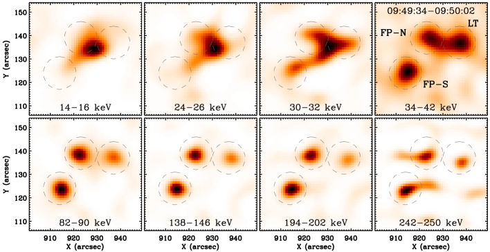
The 2003 November 3 solar flare of X3.9 class (Solar Object Locator: SOL2003-11-03T09:43) is an intense solar eruptive event close to the west solar limb. The unusually bright HXR emission from the coronal LT source, detectable up to 100–150 keV along with two FP sources by RHESSI (Chen & Petrosian, 2012), makes this event particularly suitable for our purpose to determine the SA model characteristics.
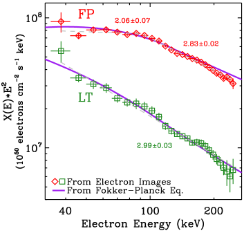
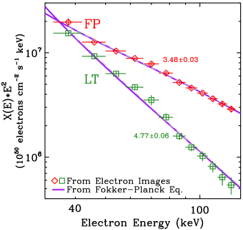
Figure 1 shows the regularized electron flux spectral images. The LT and FP sources are clearly visible up to 250 keV, about twice the highest photon energy for the LT source. We then extract the volume integrated radiating electron flux spectra above 34 keV from the LT source and the two FP sources (Figure 2, left panel). The LT spectrum can be fitted by a power law with an index 3.0, while the flatter FP spectrum can be better fitted by a broken power law with the indices 2.1 and 2.8 below and above the break energy 91 keV, respectively.
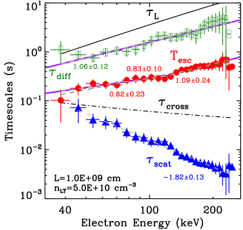
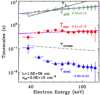
From analysis of the X-ray images (Chen & Petrosian, 2012), we obtain the density at the LT acceleration region to be cm-3 with the LT size to be cm. In Figure 2 (right panel), we plot the electron escape time and the energy diffusion time as calculated from the above spatially resolved spectra and (left panel). Except for the leftmost data point at the lowest energy, the escape time is clearly much longer than the crossing time and is 5–15 times shorter than the energy loss time . The escape time shows an overall trend increasing with energy, and can be fitted with a power law, . From the escape time, we calculate the pitch angle scattering time, which decreases with energy as . This implies a pitch angle diffusion rate of . Here we attribute the above scattering time purely to turbulence. Contribution from Coulomb collisions will be at the scale of the energy loss time and therefore negligible for electrons above 34 keV in this event. The energy diffusion time varies as and is about half the energy loss time. Thus we have the energy diffusion coefficient . The direct acceleration time is very close to the energy diffusion time. It is obvious that the energy diffusion time and pitch angle scattering time have very different energy dependences in this event.
4.3. The 2005 September 8 Event
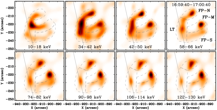
The 2005 September 8 solar flare (SOL2005-09-08T16:49) is an M2.1 class event occurring at the southeast quadrant of the Sun near the limb. As seen from the RHESSI HXR images and the Transition Region and Coronal Explorer (TRACE) 171 Å EUV images, the flare consists of two interacting loops, with their northern loop legs visually overlapped along the line-of-sight. Furthermore, the coronal LT source appears higher at altitude with increasing HXR energy (Chen & Petrosian, 2009). Here we model the acceleration region associated with the two loops as a single leaky box for the whole flare. We take the density and size of this single accelerator to be cm-3 and cm, respectively.
Figure 3 displays the electron flux images up to 130 keV, in which two flare loops can be clearly resolved. We extract the radiating electron flux spectra at the LT and FP sources summed over the two loops. As shown in Figure 4 (left panel), both the LT and FP spectra can be well fitted by a power law, with the indices 4.8 and 3.5, respectively, the difference of which is larger than that in the 2003 November 3 flare. Due to the relatively softer LT source in this event, all the model timescales are flatter than those in the 2003 November 3 flare. As in Figure 4 (right panel), the escape time can be fitted with a power law, . The scattering time varies as , and the pitch angle diffusion rate as . The energy diffusion time and acceleration time can be fitted with a similar power law, . The energy diffusion coefficient is found to be . Again, the energy dependences for the energy diffusion time and the pitch angle scattering time are very different, but now the difference is smaller than that in the 2003 November 3 flare.
4.4. Numerical Verification
For the above two events, we also use the power law forms of the escape time and the energy diffusion coefficient determined directly from observations as input to the steady state leaky box Fokker-Planck Equation (1), and solve for the electron spectra numerically using the Chang-Cooper finite difference scheme (Chang & Cooper, 1970; Park & Petrosian, 1996). We then calculate the effective thick target radiating spectra for the escaping particles. As shown in Figures 2 and 4, these numerical model spectra in general agree very well with the observed spectra from RHESSI. This is a mere self-consistency check justifying our procedure.
5. Summary and Discussions
Following our earlier paper (Petrosian & Chen, 2010), we have developed a new method for the determination of the energy dependences of basic characteristics of the SA mechanism. The particle spectrum is determined by three such characteristics, but only two of them, namely the momentum and pitch angle diffusion coefficients ( and ), play a major role. As is well known, for a nearly isotropic particle distribution at a homogeneous acceleration region, the diffusion equation in the momentum space reduces to the so-called leaky box Fokker-Planck equation, including the energy diffusion coefficient and direct acceleration rate ( and related to ) and escape time ( related to ). We show that from the observed spectra of the accelerated and escaping particles, we can determine these two unknowns of the SA mechanism by inversion of the particle acceleration and transport equations and thus gain insight into the properties of the required plasma waves or turbulence. It should be noted that, in contrast to the usual forward fitting method, this is a non-parametric method of relating the acceleration coefficients directly to observables.
In this paper we have applied the above procedure to acceleration of electrons in solar flares based on RHESSI HXR observations, assuming mainly SA by turbulence with negligible contribution to acceleration from electric fields or shocks.444In a companion paper (V. Petrosian & Q. Chen, in preparation), we explore the application of this method to acceleration of electrons in supernova remnant shocks. Here we also employ the regularized inversion procedure of Piana et al. (2007) to produce the electron flux spectral images from the RHESSI count visibilities, thus relating the acceleration model coefficients directly and non-parametrically to the raw RHESSI data.
We have applied our method to two intense flares observed by RHESSI on 2003 November 3 (X3.9 class) and 2005 September 8 (M2.1 class). The results from both events exhibit some interesting behaviors, as summarized below.
We find that electrons stay at the acceleration region much longer than the free crossing time and shorter than the energy loss time (see also Petrosian & Chen, 2010; Simões & Kontar, 2013). Furthermore, the escape time increases with energy. This is our most robust result and is independent of the details of the acceleration mechanisms. The only assumption is that electrons are accelerated at the LT region and lose most of their energy by Coulomb collisions at the FPs. The twofold effects of a long escape time, which increases the acceleration efficiency and suppresses the escaping rate, can naturally explain the relatively flat accelerated electron spectrum at the LT source, especially for the 2003 November 3 flare.
A short scattering time is a possible explanation of this observation and would justify the assumption of the pitch angle isotropy. Our results indicate that Coulomb scattering is not efficient enough to produce this effect, thus scattering by turbulence is the most likely mechanism as advocated in the SA model.
If we assume that the pitch angle scattering is the cause of the long escape time (Assumption I), then using the simple random walk relation, we find a scattering time that decreases relatively rapidly with energy and is much shorter than the crossing time (and all other times), as required in this scenario.
If we also assume the SA model (Assumption II), in which and are related by Equation (3), then we find that the energy diffusion time increases with energy and is roughly parallel to the escape time for both flares (except in the few low energy bins). The same is true for the direct acceleration time. This behavior is what is expected when the FP sources are stronger than the LT source ().
Clearly knowledge thus gained from observations can then be used to directly compare with theoretical model predictions. It should, however, be emphasized that the derivation of the electron escape time does not involve assumptions about any specific acceleration mechanisms and thus it may impose the most severe constraint on the theoretical models.
5.1. Comparison with SA Modeling
We now discuss whether the above results, specifically the discordant energy dependences of the acceleration and scattering time, can be reconciled with the predictions of the SA model. This is a test of the above Assumption II while keeping Assumption I.
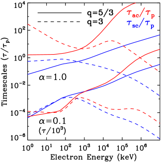
As described in the quasilinear theory, the momentum and pitch angle diffusion coefficients are related to the turbulence energy density spectrum , where is the wave number, plasma dispersion relation , and resonance conditions (e.g., Schlickeiser, 1989; Dung & Petrosian, 1994). In the relativistic range, we expect similar energy dependences for the momentum diffusion and pitch angle scattering timescales, , where is the Alfvén speed. In the non-relativistic regime of interest here, the relation becomes more complex. Most past works in the literature modeling the SA mechanism in solar flares assume plasma waves propagating parallel to the large scale magnetic fields (e.g., Steinacker & Miller, 1992; Dung & Petrosian, 1994; Pryadko & Petrosian, 1997, 1998; Petrosian & Liu, 2004). As shown in Figure 5, there is a considerable variation of the model timescales at low energies, especially for the energy diffusion (or direct acceleration) time. The scattering time from the models increases or is nearly constant with energy at the non-relativistic regime. It generally obeys an approximate relation, (Petrosian & Liu, 2004), so that a steep turbulence spectrum with is needed for a scattering time that decreases with energy. Thus, for the two flares studied above, we need and , respectively. However, for such steep turbulence spectra, the diffusion and acceleration timescales will most likely decrease with energy. Petrosian & Liu (2004) provided another approximate expression, , which is valid in a limited non-relativistic range. This would disagree with our results under the random walk approximation.
We therefore conclude that the observational results from the intense X3.9 class flare on 2003 November 3 is not consistent with the SA model predictions as presented above. While the results from the weaker M2.1 class flare on 2005 September 8 with weaker and softer LT emission have less severe disagreement with the SA model if electrons are interacting with a steep portion of the turbulence spectrum, possibly in the damping range beyond the inertial range555Recently, a steep turbulence spectrum () in the damping range has been adopted by Li et al. (2013) to explain the spectral hardening of HXR spectra above 300 keV in solar flares involving a termination shock. (Petrosian & Chen, 2010; Petrosian, 2012). However, a steep turbulence spectrum will require more energy in the turbulence unless its spectral range of the steep part is narrow. Obliquely propagating waves will have different energy dependences for these timescales, but limited information on perpendicularly propagating waves seems to give similar energy dependences for the momentum and pitch angle diffusion timescales (Pryadko & Petrosian, 1999).
We should emphasize that the two intense events on 2003 November 3 and 2005 September 8 are not representative of typical flares. As mentioned above, the escape time and energy diffusion time are primarily determined by the ratio . The discrepancy between the above observational results and the SA model predictions is related to the relatively bright LT source with a flat spectrum. On the contrary, imaging spectroscopic observations have indicated that for most flares, the LT source is much weaker and has a steeper spectrum (e.g., Petrosian et al., 2002; Liu, 2006; Shao & Huang, 2009). Furthermore, spectral studies of the over-the-limb solar flares with their FP sources occulted from Yohkoh (Tomczak, 2001, 2009) and from RHESSI (Krucker & Lin, 2008; Saint-Hilaire et al., 2008) found that their spectral index on average is larger than that from the disk flares by 1.5 and 2, respectively. Thus, for those more common flare events, we can expect flatter energy dependences for the escape time, energy diffusion time, and scattering time as determined from observations, which would be closer to the SA model predictions.
5.2. Shock Acceleration
Addition of acceleration by a shock does not seem to help in this regard. If a standing shock exists at the acceleration region with a high speed , it may dominate the acceleration rate,
| (23) |
with an acceleration time (Petrosian, 2012). If the escape of particles is again diffusive in nature (, then we expect a simple inverse relation between the escape time and shock acceleration time, .
On the other hand, if shock acceleration is dominant, then from integration of the Fokker-Planck equation (with ), we obtain
| (24) |
Therefore the acceleration rate by a shock, which now depends only on the pitch angle diffusion rate, is similar to the energy diffusion coefficient derived above (Equation 17). We can then express the shock acceleration timescale in terms of observables as . For the case , our observations indicate that roughly (Equation 22), which is in direct disagreement with the above inverse relation expected from the shock acceleration model.
Thus for both SA and shock acceleration, we encounter contradiction with the above Assumption I that the long escape time is due to the random walk approximation expected in the strong diffusion limit (). Alternatively, a long escape time may arise in a magnetic mirror geometry as we discuss next (e.g., Chen & Petrosian, 2012).
5.3. Weak Diffusion and Magnetic Mirroring
Assumption I involves the use of Equation (5), which in the strong diffusion limit gives the random walk relation, but in the weak diffusion limit () gives . However, in addition to plasma waves or turbulence, magnetic reconnection may restructure the the large scale magnetic fields into a configuration that can also trap and accelerate particles in the LT region (e.g., Somov & Kosugi, 1997; Karlický & Kosugi, 2004; Minoshima et al., 2011; Grady et al., 2012). The newly reconnected, cusp-shaped magnetic field lines relax and shrink to the underlying closed loops and may form a magnetic mirror geometry in the corona. A cusp-shaped geometry is often seen from soft X-ray and EUV images and coronal HXR sources in many events have been found to be located near such a structure (e.g., Sun et al., 2012; Liu et al., 2013).
If the magnetic field lines converge from the center of the LT acceleration region to where the particles escape into the loop legs, then the escape time will be affected. In the strong diffusion limit we would still expect a random walk process. While in the weak diffusion limit, instead of , we expect an escape time , which is the time needed to scatter particles into the loss cone (Kennel, 1969; Melrose & Brown, 1976). The proportionality constant depends on several factors but primarily on the pitch angle distribution and the mirroring ratio , the ratio of the magnetic field intensity from the boundary to the center of the acceleration region. As well known from the conservation of the magnetic moment (the first adiabatic invariant), only particles with a pitch angle smaller than the mirroring angle, or a pitch angle cosine , can escape from this magnetic trap and penetrate to the loop FPs. In absence of scattering, the rest of the particles will be trapped in the mirror. But when there is scattering, the particles with high pitch angles will be scattered into the loss cone, perhaps after several bounces back and forth between the mirroring points. For example, for an isotropic pitch angle distribution, we can obtain an average escape time as
| (25) |
which for strong convergence ) would give . Malyshkin & Kulsrud (2001) showed that for electrons injected into the trap with , one has a proportionality constant of . For strong convergence, they also identified an intermediate range , where .
In summary, in a converging field geometry, we expect the escape time first decreases with an increasing scattering time, but instead of becoming equal to the crossing time, it then reaches a minimum and begins to increase linearly with the scattering time when the latter exceeds the crossing time. Thus, a long escape time can arise not only from a short scattering time in the strong diffusion scenario, but also from a long scattering time in a converging magnetic field configuration. Some earliest mechanisms that were proposed to produce a distinct coronal HXR source (e.g., Leach, 1984; Fletcher & Martens, 1998) basically adopted the second scenario with Coulomb collisions as the scattering agent for the suprathermal electrons. In addition, an observed escape time that increases with energy requires a scattering time that also increases with energy. For scattering due to Coulomb collisions in a fully ionized hydrogen plasma in the non-relativistic limit, the electron pitch angle scattering time follows (Trubnikov, 1965; Melrose & Brown, 1976; Bai, 1982; Aschwanden, 2002).
Therefore, if Coulomb scattering is the agent that scatters electrons into the loss cone and cause their escape, the escape time will be comparable to the energy loss time and scales with energy as . This is in disagreement with the above observational results from both events. Even if the scattering time is comparable to the crossing time, then we would be in the intermediate regime and the escape time would vary like the crossing time as , which also disagrees with observations.
On the other hand, if scattering is dominated by wave-particle interactions, then because the above observations gives roughly similar energy dependences for the energy diffusion time and escape time, this would mean similar dependences for the scattering time and energy diffusion time. This would be in better agreement with theoretical expectations in the SA model by turbulence. But for the shock acceleration model, our observations imply a relation , and in a converging field configuration, we expect . While the shock acceleration model predicts (Section 5.2).
We therefore conclude that this very first non-parametric determination of the SA model characteristics directly from the observed data could be reconciled with stochastic acceleration by turbulence, if the LT acceleration region is surrounded by a cusp-shaped magnetic geometry with a relatively large mirroring ratio. On the other hand, our results do not seem to be consistent with what is expected in acceleration in a standing shock at the LT region of the flare, regardless of whether there is strong field convergence. The exact treatment of the acceleration and transport of electrons in a more realistic geometry cannot be treated by the leaky box model and requires inclusion of the kinematic effects of a magnetic mirror in a dynamic flare environment that is more complicated and will be treated in future works.
References
- Aschwanden (2002) Aschwanden, M. J. 2002, Space Sci. Rev., 101, 1
- Bai (1982) Bai, T. 1982, ApJ, 259, 341
- Barbosa (1979) Barbosa, D. D. 1979, ApJ, 233, 383
- Battaglia & Benz (2006) Battaglia, M., & Benz, A. O. 2006, A&A, 456, 751
- Bian et al. (2012) Bian, N., Emslie, A. G., & Kontar, E. P. 2012, ApJ, 754, 103
- Brown (1971) Brown, J. C. 1971, Sol. Phys., 18, 489
- Brown et al. (2006) Brown, J. C., Emslie, A. G., Holman, G. D., et al. 2006, ApJ, 643, 523
- Bykov & Fleishman (2009) Bykov, A. M., & Fleishman, G. D. 2009, ApJ, 692, L45
- Chandrasekhar (1943) Chandrasekhar, S. 1943, Reviews of Modern Physics, 15, 1
- Chang & Cooper (1970) Chang, J. S., & Cooper, G. 1970, J. Comp. Phys., 6, 1
- Chen & Petrosian (2009) Chen, Q., & Petrosian, V. 2009, AGU Fall Meeting Abstracts, SH23A1523
- Chen & Petrosian (2012) Chen, Q., & Petrosian, V. 2012, ApJ, 748, 33
- Codispoti et al. (2013) Codispoti, A., Torre, G., Piana, M., & Pinamonti, N. 2013, ApJ, 773, 121
- Dennis (1988) Dennis, B. R. 1988, Sol. Phys., 118, 49
- Dung & Petrosian (1994) Dung, R., & Petrosian, V. 1994, ApJ, 421, 550
- Emslie et al. (2004) Emslie, A. G., Miller, J. A., & Brown, J. C. 2004, ApJ, 602, L69
- Emslie et al. (2012) Emslie, A. G., Dennis, B. R., Shih, A. Y., et al. 2012, ApJ, 759, 71
- Fermi (1949) Fermi, E. 1949, Phys. Rev., 75, 1169
- Fleishman & Toptygin (2013) Fleishman, G. D., & Toptygin, I. N. 2013, MNRAS, 429, 2515
- Fletcher & Martens (1998) Fletcher, L., & Martens, P. C. H. 1998, ApJ, 505, 418
- Grady et al. (2012) Grady, K. J., Neukirch, T., & Giuliani, P. 2012, A&A, 546, A85
- Grigis & Benz (2006) Grigis, P. C., & Benz, A. O. 2006, A&A, 458, 641
- Guo et al. (2013) Guo, J., Emslie, A. G., & Piana, M. 2013, ApJ, 766, 28
- Hamilton & Petrosian (1992) Hamilton, R. J., & Petrosian, V. 1992, ApJ, 398, 350
- Holman (2012) Holman, G. D. 2012, Physics Today, 65, 56
- Holman et al. (2003) Holman, G. D., Sui, L., Schwartz, R. A., & Emslie, A. G. 2003, ApJ, 595, L97
- Holman et al. (2011) Holman, G. D., Aschwanden, M. J., Aurass, H., et al. 2011, Space Sci. Rev., 159, 107
- Hurford et al. (2002) Hurford, G. J., Schmahl, E. J., Schwartz, R. A., et al. 2002, Sol. Phys., 210, 61
- Ishikawa et al. (2011) Ishikawa, S., Krucker, S., Takahashi, T., & Lin, R. P. 2011, ApJ, 737, 48
- Johns & Lin (1992) Johns, C. M., & Lin, R. P. 1992, Sol. Phys., 137, 121
- Karlický & Kosugi (2004) Karlický, M., & Kosugi, T. 2004, A&A, 419, 1159
- Kennel (1969) Kennel, C. F. 1969, Rev. Geophys. Space Phys., 7, 379
- Kennel & Engelmann (1966) Kennel, C. F., & Engelmann, F. 1966, Physics of Fluids, 9, 2377
- Kontar et al. (2005) Kontar, E. P., Emslie, A. G., Piana, M., Massone, A. M., & Brown, J. C. 2005, Sol. Phys., 226, 317
- Krucker et al. (2008a) Krucker, S., Hurford, G. J., MacKinnon, A. L., Shih, A. Y., & Lin, R. P. 2008a, ApJ, 678, L63
- Krucker & Lin (2008) Krucker, S., & Lin, R. P. 2008, ApJ, 673, 1181
- Krucker et al. (2008b) Krucker, S., Battaglia, M., Cargill, P. J., et al. 2008b, A&A Rev., 16, 155
- Leach (1984) Leach, J. 1984, PhD thesis, Stanford Univ.
- Li et al. (2013) Li, G., Kong, X., Zank, G., & Chen, Y. 2013, ApJ, 769, 22
- Lin (1974) Lin, R. P. 1974, Space Sci. Rev., 16, 189
- Lin & Hudson (1976) Lin, R. P., & Hudson, H. S. 1976, Sol. Phys., 50, 153
- Lin et al. (2002) Lin, R. P., Dennis, B. R., Hurford, G. J., et al. 2002, Sol. Phys., 210, 3
- Lin et al. (2003) Lin, R. P., Krucker, S., Hurford, G. J., et al. 2003, ApJ, 595, L69
- Liu et al. (2006) Liu, S., Petrosian, V., & Mason, G. M. 2006, ApJ, 636, 462
- Liu (2006) Liu, W. 2006, PhD thesis, Stanford Univ.
- Liu et al. (2013) Liu, W., Chen, Q., & Petrosian, V. 2013, ApJ, 767, 168
- Liu et al. (2008) Liu, W., Petrosian, V., Dennis, B. R., & Jiang, Y. W. 2008, ApJ, 676, 704
- Liu et al. (2009) Liu, W., Petrosian, V., & Mariska, J. T. 2009, ApJ, 702, 1553
- Longair (1992) Longair, M. S. 1992, High Energy Astrophysics. Vol. 1: Particles, Photons and their Detection (Cambridge: Cambridge Univ. Press)
- Malyshkin & Kulsrud (2001) Malyshkin, L., & Kulsrud, R. 2001, ApJ, 549, 402
- Markwardt (2009) Markwardt, C. B. 2009, in ASP Conf. Ser., Vol. 411, Astronomical Data Analysis Software and Systems XVIII, ed. D. A. Bohlender, D. Durand, & P. Dowler, 251
- Massone & Piana (2013) Massone, A. M., & Piana, M. 2013, Sol. Phys., 283, 177
- Masuda et al. (1994) Masuda, S., Kosugi, T., Hara, H., Tsuneta, S., & Ogawara, Y. 1994, Nature, 371, 495
- Melrose (1974) Melrose, D. B. 1974, Sol. Phys., 37, 353
- Melrose (2009) Melrose, D. B. 2009, Encyclopedia of Complexity and Systems Science, Part 1, ed. R. A. Meyers (Berlin: Springer), 21; arXiv:0902.1803
- Melrose & Brown (1976) Melrose, D. B., & Brown, J. C. 1976, MNRAS, 176, 15
- Miller (1997) Miller, J. A. 1997, ApJ, 491, 939
- Miller et al. (1996) Miller, J. A., Larosa, T. N., & Moore, R. L. 1996, ApJ, 461, 445
- Miller & Roberts (1995) Miller, J. A., & Roberts, D. A. 1995, ApJ, 452, 912
- Miller et al. (1997) Miller, J. A., Cargill, P. J., Emslie, A. G., et al. 1997, J. Geophys. Res., 102, 14631
- Minoshima et al. (2011) Minoshima, T., Masuda, S., Miyoshi, Y., & Kusano, K. 2011, ApJ, 732, 111
- Moré (1977) Moré, J. 1977, in Lecture Notes in Mathematics, Vol. 630, Numerical Analysis, ed. G. A. Watson (Springer-Verlag), 105
- Park & Petrosian (1995) Park, B. T., & Petrosian, V. 1995, ApJ, 446, 699
- Park & Petrosian (1996) Park, B. T., & Petrosian, V. 1996, ApJS, 103, 255
- Park et al. (1997) Park, B. T., Petrosian, V., & Schwartz, R. A. 1997, ApJ, 489, 358
- Petrosian (1973) Petrosian, V. 1973, ApJ, 186, 291
- Petrosian (2012) Petrosian, V. 2012, Space Sci. Rev., 173, 535
- Petrosian & Chen (2010) Petrosian, V., & Chen, Q. 2010, ApJ, 712, L131
- Petrosian & Donaghy (1999) Petrosian, V., & Donaghy, T. Q. 1999, ApJ, 527, 945
- Petrosian et al. (2002) Petrosian, V., Donaghy, T. Q., & McTiernan, J. M. 2002, ApJ, 569, 459
- Petrosian & Liu (2004) Petrosian, V., & Liu, S. 2004, ApJ, 610, 550
- Piana et al. (2007) Piana, M., Massone, A. M., Hurford, G. J., et al. 2007, ApJ, 665, 846
- Piana et al. (2003) Piana, M., Massone, A. M., Kontar, E. P., et al. 2003, ApJ, 595, L127
- Prato et al. (2009) Prato, M., Emslie, A. G., Kontar, E. P., Massone, A. M., & Piana, M. 2009, ApJ, 706, 917
- Pryadko & Petrosian (1997) Pryadko, J. M., & Petrosian, V. 1997, ApJ, 482, 774
- Pryadko & Petrosian (1998) Pryadko, J. M., & Petrosian, V. 1998, ApJ, 495, 377
- Pryadko & Petrosian (1999) Pryadko, J. M., & Petrosian, V. 1999, ApJ, 515, 873
- Ramaty (1979) Ramaty, R. 1979, in AIP Conf. Ser., Vol. 56, Particle Acceleration Mechanisms in Astrophysics, ed. J. Arons, C. McKee, & C. Max, 135
- Ryan & Lee (1991) Ryan, J. M., & Lee, M. A. 1991, ApJ, 368, 316
- Saint-Hilaire et al. (2008) Saint-Hilaire, P., Krucker, S., & Lin, R. P. 2008, Sol. Phys., 250, 53
- Schlickeiser (1989) Schlickeiser, R. 1989, ApJ, 336, 243
- Schmahl et al. (2007) Schmahl, E. J., Pernak, R. L., Hurford, G. J., Lee, J., & Bong, S. 2007, Sol. Phys., 240, 241
- Shao & Huang (2009) Shao, C., & Huang, G. 2009, ApJ, 691, 299
- Simões & Kontar (2013) Simões, P. J. A., & Kontar, E. P. 2013, A&A, 551, A135
- Smith et al. (2002) Smith, D. M., Lin, R. P., Turin, P., et al. 2002, Sol. Phys., 210, 33
- Somov & Kosugi (1997) Somov, B. V., & Kosugi, T. 1997, ApJ, 485, 859
- Steinacker & Miller (1992) Steinacker, J., & Miller, J. A. 1992, ApJ, 393, 764
- Sturrock (1966) Sturrock, P. A. 1966, Phys. Rev., 141, 186
- Sui & Holman (2003) Sui, L., & Holman, G. D. 2003, ApJ, 596, L251
- Sui et al. (2004) Sui, L., Holman, G. D., & Dennis, B. R. 2004, ApJ, 612, 546
- Sun et al. (2012) Sun, X., Hoeksema, J. T., Liu, Y., Chen, Q., & Hayashi, K. 2012, ApJ, 757, 149
- Syrovat-Skii & Shmeleva (1972) Syrovat-Skii, S. I., & Shmeleva, O. P. 1972, Soviet Ast., 16, 273
- Tomczak (2001) Tomczak, M. 2001, A&A, 366, 294
- Tomczak (2009) Tomczak, M. 2009, A&A, 502, 665
- Torre et al. (2012) Torre, G., Pinamonti, N., Emslie, A. G., et al. 2012, ApJ, 751, 129
- Trubnikov (1965) Trubnikov, B. A. 1965, Reviews of Plasma Physics, 1, 105
- Tsytovich (1966) Tsytovich, V. N. 1966, Soviet Phys. Uspekhi, 9, 370
- Tsytovich (1977) Tsytovich, V. N. 1977, Theory of Turbulent Plasma (New York: Pergamon)
- Tverskoǐ (1967) Tverskoǐ, B. A. 1967, Soviet Phys. JETP, 25, 317
- Tverskoǐ (1968) Tverskoǐ, B. A. 1968, Soviet Phys. JETP, 26, 821
- Wang et al. (2007) Wang, T., Sui, L., & Qiu, J. 2007, ApJ, 661, L207