Multiple Vectors Propagation of Epidemics in Complex Networks

Abstract.  This letter investigates the epidemic spreading in two-vectors propagation network (TPN). We propose detailed theoretical analysis that allows us to accurately calculate the epidemic threshold and outbreak size. It is found that the epidemics can spread across the TPN even if two sub-single-vector propagation networks (SPNs) of TPN are well below their respective epidemic thresholds. Strong positive degree-degree correlation of nodes in TPN could lead to a much lower epidemic threshold and a relatively smaller outbreak size. However, the average similarity between the neighbors from different SPNs of nodes has no effect on the epidemic threshold and outbreak size.

Keyword.  Multiple-vectors propagation, Single-vector propagation, Epidemic threshold, Outbreak size, Percolation theory.

§1   Introduction

In recent years, various types of epidemics have occurred frequently and spread around the world, causing not only a great economic loss, but also widespread public alarm. For example, the intense outbreak of SARS caused 8,098 reported cases and 774 deaths. Within weeks, SARS spread from Hong Kong to infect individuals in 37 countries in early 2003 [1]. An outbreak of mobile viruses occurred in China in 2010. The ‘Zombie’ virus attacked more than 1 million smart phones, and created a loss of $300,000 per day [2]. And we have also witnessed how social networks being used for citizens to share information and gain international support in the Arab Spring [3]. In view of these situations, it is thus urgent and essential to have a better understanding of epidemic process, and to design effective and efficient mechanisms for the restraint or acceleration of epidemic spreading.

Valid epidemic spreading models can be used to estimate the scale of a epidemic outbreak before it actually occurs in reality and evaluate new and/or improved countermeasures for the restraint or acceleration of epidemic spreading. In the last decade, there have been extensive studies on the modeling of epidemic dynamics [4-10] and various protection strategies have been proposed and evaluated [11-17]. However, these existing researches have been dominantly focusing on the cases that epidemics spread through only one vector. While in reality, many epidemics can spread through multiple vectors simultaneously. For example, it has been well recognized that AIDS can be transmitted via vectors such as sexual activity, blood and breast milk; rumor or information can be spread among groups through verbal communication and social networks; malwares can move to computers by P2P file share, email, random-scanning or instant messenger [18]; some mobile malwares can even attack smart phones through both short messaging service and bluetooth at the same time [19]. In this letter, epidemic spreading via only one vector and that through various vectors are called single-vector propagation and multiple-vectors propagation respectively. Obviously, the range and intensity of the multiple-vectors propagation will be greater than the traditional single-vector propagation. Besides, different propagation vectors can form different propagation networks and these propagation networks may have different topological characteristics and epidemic dynamics. Based on the above analysis, the study of multiple-vectors propagation of epidemics is definitely a very meaningful and necessary thing.

To the best of our knowledge, a theory describing the multiple-vectors propagation of epidemics has not been fully developed yet. In this letter, we propose and evaluate two-vectors propagation of epidemics in a two-vectors propagation network (TPN) following the typical Susceptible-Infected-Removed (SIR) model [6,7]. We map the SIR model into bond percolation [7] and develop equations which allow accurate calculations of epidemic threshold [6] and outbreak size [6] of the TPN. It is obviously found the epidemic can spread across the TPN even when the two sub-single-vector propagation networks (SPNs) of TPN are well below their respective epidemic thresholds. We also introduce two quantities for measuring the level of inter-similarity between the two SPNs. One is ASN, which measures the average similarity between the neighbors from different SPNs of nodes in the TPN. We find that epidemic threshold and outbreak size are not significantly affected by the ASN. The second quantity is DDC which describes the degree-degree correlation of nodes in different SPNs. Positive values of DDC indicate that high degree nodes in one SPN are also high degree nodes in the other SPN and vise versa. It is found that strong positive DDC leads to a clearly lower epidemic threshold and a relatively smaller outbreak size, independent of the topological characteristics of the two SPNs.

§2   Models and analysis

2.1 Network model

In this section, we propose a two-vectors propagation network (TPN) which is superposed by two sub-single-vector propagation networks (SPNs), but it is easily to extend the model to an arbitrary number of SPNs with any size.

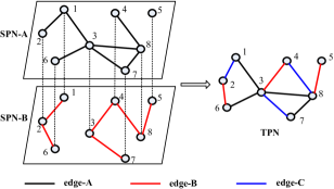
Figure 1: TPN is a superposition network of SPN-A and SPN-B.

As shown in Fig.1, two different spread vectors, vector-A and vector-B form two SPNs, SPN-A and SPN-B respectively. These two SPNs have same nodes, but different topologies. When an epidemic can spread through these two vectors at the same time, the real propagation network of this epidemic are the TPN (right-hand chart) which is superposed by SPN-A and SPN-B. Thus, a node in TPN may be infected by one vector even though it cannot be infected via the other one, or it may be infected by these two vectors at the same time. Each node in the TPN has up to three types of edges where the edge-A belongs to SPN-A, the edge-B belongs to SPN-B, and the edge-C belongs to both SPN-A and SPN-B. Vector degree $k_{M}\equiv(k_{A}-k_{C},k_{B}-k_{C},k_{C})$ is used to characterize the node of TPN, where $k_{A}-k_{C}$, $k_{B}-k_{C}$ and $k_{C}$ represent the numbers of edge-A, edge-B and edge-C, respectively. The numerical value of vector degree of node in TPN is defined by $|k_{M}|=k_{A}+k_{B}-k_{C}$. For instance, the vector degree of node 3 of Fig.1 is $k_{M}\equiv(4-1,2-1,1)$.

Actually, in the vector degree of node in TPN, $k_{C}$ evaluates how many neighbors of a node in SPN-A are also its neighbors in SPN-B which can affect the topology of TPN. We develop a measure, $\alpha$, called ASN to assess the average similarity between the neighbors from different SPNs of nodes in the TPN and it is defined as

$$\alpha=\frac{\sum\limits_{i}{k_{C}}(i)}{\sum\limits_{i}{|k_{M}}(i)|},$$ (1)

where ${k_{C}}(i)$ and $|k_{M}(i)|$ are the values of $k_{C}$ and $|k_{M}|$ of node $i$ in TPN, respectively. For increasing values of $\alpha$ more of the neighbors of a node in SPN-A are also its neighbors in SPN-B and these two SPNs become more similar. For $\alpha=1$, these two SPNs must be identical.

For a node of TPN, it may be a high degree node in SPN-A and a low degree one in SPN-B, or a high degree node in SPN-A and also a high degree one in SPN-B. The influence of different combinations of nodes degrees in the two SPNs for the characteristics of two-vectors propagation of epidemics is one of our main research problems. Analogously to the degree correlation in a single network [20,21] and the network assortativity in interconnected networks [10], we define the degree-degree correlation (DDC) of nodes in two SPNs as follows

$$\beta=\frac{\sum\limits_{k_{A}}\sum\limits_{k_{B}}(k_{A}k_{B}(p(k_{A},k_{B})-(\sum\limits_{k_{A}}p(k_{A},k_{B}))(\sum\limits_{k_{B}}p(k_{A},k_{B}))))}{\sum\limits_{k_{B}}k_{B}^{2}\sum\limits_{k_{A}}p(k_{A},k_{B})-(\sum\limits_{k_{B}}k_{B}\sum\limits_{k_{A}}p(k_{A},k_{B}))^{2}},$$ (2)

where $p(k_{A},k_{B})$ denotes the probability that a randomly chosen node in TPN has degree $k_{A}$ in SPN-A and $k_{B}$ in SPN-B. These two SPNs are said to be disassortative if $\beta<0$, assortative if $\beta>0$, and uncorrelated if $\beta=0$.

2.2 Epidemic spreading model

The epidemic spreading model adopted here is the Susceptible-Infected-Removed (SIR) model which is the most basic and well-studied epidemic spreading model [6,7]. In the SIR model, the individuals of the network can be divided into three compartments, including susceptibles (S, those who are prone to be infected), infectious (I, those who have been infected), and recovered (R, those who have recovered from the disease). At each time step, a susceptible node becomes infected with probability $\lambda$ if it is directly connected to a infected node. The parameter $\lambda$ is called the spreading rate. Meanwhile, an infected node becomes a recovered node with probability $\delta$. For the proposed two-vectors propagation model, we assume that a susceptible node becomes infected with probabilities $\lambda_{A}$,$\lambda_{B}$ and $\lambda_{C}$ if it is directly connected to one infected node through edge-A, edge-B and edge-C, respectively. Obviously, $\lambda_{C}=1-(1-\lambda_{A})(1-\lambda_{B})$. Meanwhile, an infected node becomes a recovered node with probability $\delta$. Without loss of generality, we let $\delta=1$.

2.3 Calculations of epidemic threshold

Traditionally the percolation process [7] is parametrized by a probability $\varphi$, which is the probability that a node is functioning in the network. In technical terms of percolation theory, one says that the functional nodes are occupied and $\varphi$ is called the occupation probability. With only slight modification the general SIR model can be perfectly mapped into the bond percolation in complex networks where spreading rate corresponds to the probability that a link is occupied in percolation [7,10]. We now use the SIR model and the bond percolation theory to analyze the two-vectors propagation of epidemics in the defined TPN. For the two-vectors propagation model, three types of edges are occupied at the probabilities of $\lambda_{A}$,$\lambda_{B}$ and $\lambda_{C}$ respectively. Let $h_{A}(x)$ ($h_{B}(x)$, $h_{C}(x)$) be the generating function [21,22] for the distribution of the sizes of components which are reached by an edge with type of edge-A (edge-B, edge-C) and following it to one of its ends. Later the size of components formed by infected nodes will be called the outbreak size.

$$\begin{split}h_{A}(x)=1-\lambda_{A}+x\lambda_{A}\times\frac{\sum\limits_{k_{M},\ k_{A}-k_{C}\geq 1}|k_{M}|p_{k_{M}}h_{A}^{k_{A}-k_{C}-1}(x)h_{B}^{k_{B}-k_{C}}(x)h_{C}^{k_{C}}(x)}{\sum\limits_{k_{M}}|k_{M}|p_{k_{M}}},\ \ \end{split}$$ (3)

$$\begin{split}h_{B}(x)=1-\lambda_{B}+x\lambda_{B}\times\frac{\sum\limits_{k_{M},\ k_{B}-k_{C}\geq 1}|k_{M}|p_{k_{M}}h_{A}^{k_{A}-k_{C}}(x)h_{B}^{k_{B}-k_{C}-1}(x)h_{M}^{k_{C}}(x)}{\sum\limits_{k_{M}}|k_{M}|p_{k_{M}}},\end{split}$$ (4)

$$\begin{split}h_{C}(x)=1-\lambda_{C}+x\lambda_{C}\times\frac{\sum\limits_{k_{M},\ k_{C}\geq 1}|k_{M}|p_{k_{M}}h_{A}^{k_{A}-k_{C}}(x)h_{B}^{k_{B}-k_{C}}(x)h_{M}^{k_{C}-1}(x)}{\sum\limits_{k_{M}}|k_{M}|p_{k_{M}}},\end{split}$$ (5)

where $p_{k_{M}}$ denotes the probability that a randomly chosen node of TPN has the vector degree $k_{M}$.

Generally, an epidemic always starts from a network node, not an edge, therefore we proceed to analyze the outbreak size distribution for epidemic sourced from a randomly selected node. If we start at a randomly chosen node in TPN, then we have one such outbreak size at the end of each edge leaving that node, and hence the generating function for the outbreak size caused by a network node is

$$\centering{H(x)=x\times\sum\limits_{k_{M}}p_{k_{M}}h_{A}^{k_{A}-k_{C}}(x)h_{B}^{k_{B}-k_{C}}(x)h_{C}^{k_{C}}(x).}\@add@centering$$ (6)

Although it is not usually possible to find a closed-form expression for the complete distribution of outbreak size in a network, we can find closed-form expressions for the average outbreak size of an epidemic in TPN from Eqs.(6). This average outbreak size can be derived by taking derivates of Eqs.(6) at $x=1$, we have

$$\begin{split}<s>=H^{\prime}(1)=1+\sum\limits_{k_{M}}p_{k_{M}}(k_{A}-k_{C})h^{\prime}_{A}(1)+\ \ \ \ \ \ \ \ \ \ \ \ \ \ \ \ \ \ \ \ \ \ \ \ \ \ \ \ \ \\ \sum\limits_{k_{M}}p_{k_{M}}(k_{B}-k_{C})h^{\prime}_{B}(1)+\sum\limits_{k_{M}}p_{k_{M}}k_{C}h^{\prime}_{C}(1).\end{split}$$ (7)

In Eq.(7), functions $h^{\prime}_{A}(1)$, $h^{\prime}_{B}(1)$ and $h^{\prime}_{C}(1)$ can be derived from Eqs.(3)-(5). Taking derivatives on both sides of Eqs.(3)-(5) at $x=1$, we have

$$h^{\prime}_{A}(1)=\lambda_{A}+\lambda_{A}<k_{M}>^{-1}(m_{11}h^{\prime}_{A}(1)+m_{12}h^{\prime}_{B}(1)+m_{13}h^{\prime}_{C}(1)),$$ (8)

$$h^{\prime}_{B}(1)=\lambda_{B}+\lambda_{B}<k_{M}>^{-1}(m_{21}h^{\prime}_{A}(1)+m_{22}h^{\prime}_{B}(1)+m_{23}h^{\prime}_{C}(1)),$$ (9)

$$h^{\prime}_{C}(1)=\lambda_{C}+\lambda_{C}<k_{M}>^{-1}(m_{31}h^{\prime}_{A}(1)+m_{32}h^{\prime}_{B}(1)+m_{33}h^{\prime}_{C}(1)),$$ (10)

where

$$<k_{M}>=\sum\limits_{k_{M}}|k_{M}|p_{k_{M}},$$

$$m_{11}=\sum\limits_{k_{M},k_{A}-k_{C}\geq 1}|k_{M}|p_{k_{M}}(k_{A}-k_{C}-1),$$

$$m_{12}=\sum\limits_{k_{M},k_{A}-k_{C}\geq 1}|k_{M}|p_{k_{M}}(k_{B}-k_{C}),$$

$$m_{13}=\sum\limits_{k_{M},k_{A}-k_{C}\geq 1}|k_{M}|p_{k_{M}}k_{C},$$

$$m_{21}=\sum\limits_{k_{M},k_{B}-k_{C}\geq 1}|k_{M}|p_{k_{M}}(k_{A}-k_{C}),$$

$$m_{22}=\sum\limits_{k_{M},k_{B}-k_{C}\geq 1}|k_{M}|p_{k_{M}}(k_{B}-k_{C}-1),$$

$$m_{23}=\sum\limits_{k_{M},k_{B}-k_{C}\geq 1}|k_{M}|p_{k_{M}}k_{C},$$

$$m_{31}=\sum\limits_{k_{M},k_{C}\geq 1}|k_{M}|p_{k_{M}}(k_{A}-k_{C}),$$

$$m_{32}=\sum\limits_{k_{M},k_{C}\geq 1}|k_{M}|p_{k_{M}}(k_{B}-k_{C}),$$

$$m_{33}=\sum\limits_{k_{M},k_{C}\geq 1}|k_{M}|p_{k_{M}}(k_{C}-1).$$

From Eqs.(8)-(10), we have

$$Mh=-<k_{M}>e,$$ (11)

where

$$M=\left(\begin{array}[]{ccc}-\lambda_{A}^{-1}<k_{M}>+m_{11}&m_{12}&m_{13}\\ m_{21}&-\lambda_{B}^{-1}<k_{M}>+m_{22}&m_{23}\\ m_{31}&m_{32}&-\lambda_{C}^{-1}<k_{M}>+m_{33}\\ \end{array}\right),$$

$h=(h^{\prime}_{A}(1)\ h^{\prime}_{B}(1)\ h^{\prime}_{C}(1))^{T},$ and $\ e=(1\ 1\ 1)^{T}$. Therefore, $h^{\prime}_{A}(1)$, $h^{\prime}_{B}(1)$, $h^{\prime}_{C}(1)$ diverge at the point where

$$\emph{\emph{det}}M=0,$$ (12)

from which we can calculate the set of the epidemic thresholds $\{\lambda_{Tc}=(\lambda_{TAc},\lambda_{TBc})\}$ of the TPN.

2.4 Calculations of outbreak size

When an epidemic spread across the TPN, the infected nodes will form into a giant component. Let $u_{A}$, $u_{B}$ and $u_{C}$ be the average probabilities that a node is not connected to the giant component via the edge-A, edge-B and edge-C, respectively. According to percolation theory there are two ways this can happen: either the edge in question can be unoccupied, or it is occupied but the node at the other end of the edge is itself not a member of the giant component. The latter happens only if that node is not connected to the giant component via any of its other edges. Thus we have

$$\begin{split}u_{A}=1-\lambda_{A}+\lambda_{A}\times\frac{\sum\limits_{k_{M},\ k_{A}-k_{C}\geq 1}|k_{M}|p_{k_{M}}u_{A}^{k_{A}-k_{C}-1}u_{B}^{k_{B}-k_{C}}u_{C}^{k_{C}}}{\sum\limits_{k_{M}}|k_{M}|p_{k_{M}}},\ \ \end{split}$$ (13)

$$\begin{split}u_{B}=1-\lambda_{B}+\lambda_{B}\times\frac{\sum\limits_{k_{M},\ k_{B}-k_{C}\geq 1}|k_{M}|p_{k_{M}}u_{A}^{k_{A}-k_{C}}u_{B}^{k_{B}-k_{C}-1}u_{C}^{k_{C}}}{\sum\limits_{k_{M}}|k_{M}|p_{k_{M}}},\end{split}$$ (14)

$$\begin{split}u_{C}=1-\lambda_{C}+\lambda_{C}\times\frac{\sum\limits_{k_{M},\ k_{C}\geq 1}|k_{M}|p_{k_{M}}u_{A}^{k_{A}-k_{C}}u_{B}^{k_{B}-k_{C}}u_{C}^{k_{C}-1}}{\sum\limits_{k_{M}}|k_{M}|p_{k_{M}}}.\end{split}$$ (15)

For the whole TPN, the outbreak size, i.e. the size of the giant component can be calculated by

$$s=1-\sum\limits_{k_{M}}p_{k_{M}}u_{A}^{k_{A}-k_{C}}u_{B}^{k_{B}-k_{C}}u_{C}^{k_{C}}.$$ (16)

Note: The traditional single-vector propagation model is a special case of our proposed two-vectors propagation model. The epidemic threshold $\lambda_{A}={<k_{A}>}/({<k^{2}_{A}>-<k_{A}>})$ [7] and the outbreak size $s=1-\sum\limits_{k_{A}}p_{k_{A}}u_{A}^{k_{A}}$ [7] of single-vector propagation network can be obtained from Eq.12 and Eq.16 when $k_{B}=k_{C}=0$. That is to say, the results of this letter are applicable in a more general situation.

§3   Simulation results and discussions

In this section, we evaluate the two-vectors propagation of epidemics over the TPN by simulations. Three different types of TPN are constructed where ($i$) both of these two SPNs are scale-free (SF) networks; ($ii$) one SPN is Erdős-Rényi (ER) random network and the other one is SF network; ($iii$) both of them are ER networks. We use ‘X(a,b)’ to describe a SPN, where X is the type of network, ‘a’ is the network size and ‘b’ is the average degree. For example, SF(2000,3) denotes a SPN comprised of 2000 nodes with average degree 3. For convenience, we term these three TPNs as SF-SF, ER-SF and ER-ER, respectively.

3.1 Epidemic threshold and outbreak size

In Fig.2, the three-dimensional(3D) curved surfaces obtained by simulations, indicate the outbreak sizes for epidemic spreading corresponding to different combinations of spreading rates $(\lambda_{A},\lambda_{B})$, where $\lambda_{A}$ and $\lambda_{B}$ are the respective spreading rates of epidemic over two SPNs. The vertical fences obtained by calculating Eq.(12), represent the theoretical epidemic thresholds of the epidemic which spreads over TPN. We can see that the theoretical epidemic thresholds are accurate in judging the endemic state. It can be found obviously that an epidemic could spread across the TPN even if these two SPNs well below their respective epidemic thresholds, which is also independent of the construction of the TPN. Let $\lambda_{Ac}$ and $\lambda_{Bc}$ be the respective epidemic thresholds of two SPNs. As shown in Fig.2(a), the epidemic threshold $\lambda_{Ac}$ of SF(2000,3.997) corresponds to the epidemic threshold $(\lambda_{TAc},\lambda_{TBc})$ of SF(2000,3.997)-SF(2000,3.998) where $\lambda_{TBc}=0$, hence $\lambda_{Ac}=0.1056$. Similarly, we get $\lambda_{Bc}=0.1102$. From Fig.2 we can see that, for any epidemic threshold $(\lambda_{TAc},\lambda_{TBc})$ of SF(2000,3.997)-SF(2000,3.998) where $\lambda_{TAc}\cdot\lambda_{TBc}\neq 0$, there are $\lambda_{TAc}<\lambda_{Ac}$ and $\lambda_{TBc}<\lambda_{Bc}$.

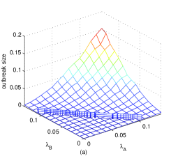
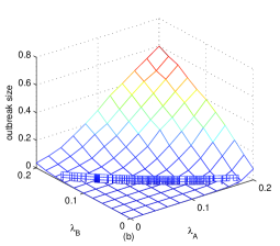
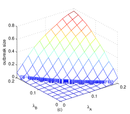
Figure 2: 3D curved surfaces obtained by simulations, indicate the outbreak sizes. The vertical fence represents the theoretical epidemic threshold. Three TPNs models are (a) SF(2000,3.997)-SF(2000,3.998); (b) ER(2000,5.883)-SF(2000,3.997) and (c) ER(2000,5.922)-ER(2000,5.965), respectively.

We now evaluate the accuracy of our theoretical derivation for the outbreak size by comparing the results obtained by theoretical analysis and simulations. There are two 3D curved surfaces in each 3D map of Figs.3(a-c), where the light one indicates the theoretical outbreak size and the dark one represents the experimental value. To get a clearer sight, three section planes of each 3D map are shown in Figs.3(d-f). We observe that theoretical calculations are in correspondence with the data of experiments.

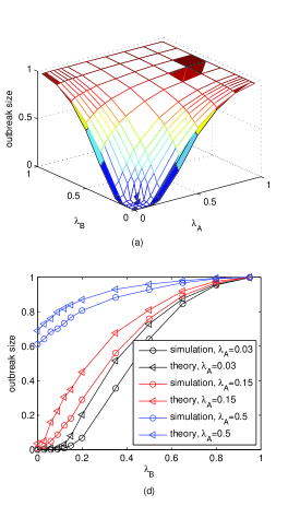
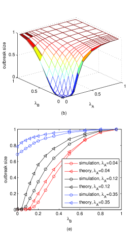
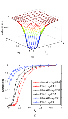
Figure 3: In (a-c), the light and dark 3D curved surfaces are the theoretical and experimental outbreak sizes, respectively. (d-f) show some corresponding section planes of (a-c). Three TPNs models are (a,d) SF(2000,3.997)-SF(2000,3.998); (b,e) ER(2000,5.883)-SF(2000,3.997) and (c,f) ER(2000,5.922)-ER(2000,5.965), respectively.

3.2 ASN and DDC

In the real world, an individual of the TPN may have some same neighbors in the two SPNs. In section 2, we used a measure ASN to assess the average similarity between the neighbors from different SPNs of nodes in the TPN. Another quantity DDC is also developed to describe the degree-degree correlation of nodes in different SPNs. Positive values of DDC indicate that high degree nodes in one SPN are also high degree nodes in the other SPN and vise versa. While the topologies of the SPNs remain unchanged, the topologies of the TPN could be affected to some degree by the ASN and DDC, and may ultimately influence the epidemic processes of the epidemic over TPN.

It is easy to achieve any targeted value of ASN for SF-SF and ER-ER. Two SF(ER)-SPNs can be obtained by preferentially(randomly) adding edges to a same SF(ER) network which has been constructed, respectively. The value of ASN is determined by the number of the edges added and the edges of the initial network. It is hard, however, to achieve a large range of ASN for ER-SF. Assume that the nodes have same tabs in each SPN, then we can get some different values of ASN for two SPNs by randomly exchanging the tabs of nodes for one SPN. In the ER-SF model, we used in Figs.4(b,e), the value of ASN roughly lies in the interval of [0.02 0.14], while for the SF-SF and ER-ER models, the corresponding intervals are all [0, 1].

In the following experiments, we assume the epidemic has same spreading rates when propagates in the two SPNs, that is $\lambda_{A}=\lambda_{B}$. As shown in Fig.4, the epidemic threshold and the outbreak size are barely affected by the ASN no matter what types of the two SPNs. This can be understood that when the topologies of the SPNs remain unchanged, high ASN means nodes can affect more of their neighbors with the large spreading rate $\lambda_{C}$, but the average number of their neighbors is relatively small. Similarly, although low ASN implies the nodes have more neighbors, most of the spreading rates between neighbors are the relatively small $\lambda_{A}$ and $\lambda_{B}$. In such cases, the average number of new infected nodes at a time step may equal no matter what the values of ASN.

Figure 4: Epidemic threshold and outbreak size for epidemic spreading in (a,d) SF-SF; (b,e) ER-SF; and (c,f) ER-ER.

Fig.5 shows the influences of DDC on the epidemic threshold and the outbreak size of the epidemics. The different values of the DDC between two SPNs are achieved by randomly exchanging the tabs of nodes of one SPN. As shown in Fig.5, a higher DDC can lead to a much lower epidemic threshold and a relatively smaller outbreak size no matter what topologies of the SPNs. The reasons can be explained as follows: high DDC means high degree nodes in one SPN are also high nodes in the other SPN and low degree nodes in one SNP also low degree nodes in the other SPN which leads to increased differences between the degrees of nodes in TPN. Instead, low DDC leads to decreased differences between the degrees of nodes in TPN. That is, high DDC makes the SF-SF and ER-SF the strengthened inhomogeneous networks and ER-ER a proximate inhomogeneous network, low DDC however makes the different types of TPNs the proximate homogeneous network. We have known that [23], the epidemic in the inhomogeneous network has a faster spread since the existence of high degree nodes and smaller outbreak size since the low degree nodes are not prone to be infected, than in the homogeneous network when these two networks have same average degree. This theory perfectly explains the results of our experiments.

Figure 5: Epidemic threshold and outbreak size for epidemic spreading in (a,d) SF(2000,3.997)-SF(2000,3.995); (b,e) ER(2000,4.005)-SF(2000,3.997); and (c,f) ER(2000,5.950)-ER(2000,5.956).

§4   Conclusions

In this letter, we demonstrated the dynamics of two-vectors propagation of epidemics over TPN . Our main contributions can be summarized as follows: (1) We presented the multiple-vectors propagation system of epidemics and derived equations to accurately calculate the epidemic threshold and outbreak size in the TPN. (2) We found that the epidemics could spread across the TPN even if two SPNs are well below their respective epidemic thresholds. (3) We proposed two quantities for measuring the level of inter-similarity between two SPNs. ASN evaluates the average similarity between the neighbors from different SPNs of nodes in the TPN which is found barely affect the epidemic threshold and outbreak size of epidemics in the TPN. DDC describes the degree-degree correlation of nodes in different SPNs. It is found that a higher DDC could lead to a much lower epidemic threshold and a relatively smaller outbreak size no matter what topologies of the SPNs.

Although we consider the epidemics spreading on TPN which superposed by only two SPNs, it is easily to extend the model to an arbitrary number of SPNs with any size. Our research not only provide useful tools and insights for further studies of dynamics of multi-vectors propagation of epidemics, but also has important implications for the design of efficient control strategies.

§5   Acknowledgement

This paper was supported by the Foundation for the Author of National Excellent Doctoral Dissertation of PR China (Grant No. 200951), the National Natural Science Foundation of China (Grant Nos. 61100204, 61170269, 61121061), the Asia Foresight Program under NSFC Grant (Grant No. 61161140320).

References

- [1] R. D. Smith, Social Science and Medicine, 63 (2006) 3113.
- [2] www.informationweek.com/news/security/attacks/228200648
- [3] P. Howard, A.Duffy, D. Freelon, M. Hussain, W. Marai, M. Mazaid, Project on Information Technology Political Islam, (2011) 1-30.
- [4] R. Pastor-Satorras, A. Vespignani, Phys. Rev. Lett. 86 (2001) 3200.
- [5] M. E. J. Newman, Phys. Rev. E 66 (2002) 016128.
- [6] A. Barrat, M. Barthélemy, and A. Vespignani, Dynamical Porcesses on Complex Networks (Cambridge University Press, Cambridge, 2008).
- [7] M. E. J. Newman, Networks: An Introduction (Oxford University Press, 2010).
- [8] A. Saumell-Mendiola, M. A. Serrano, M. Bogũá, Phys. Rev. E 86 (2012) 026106.
- [9] M. Dickison, S. Havlin, H. E. Stanley, Phys. Rev. E 85 (2012) 066109.
- [10] Y. Wang, G. Xiao, Physics Letters A 376 (2012) 2689.
- [11] Z. Dezso and A.-L. Barabasi, Phys. Rev. E 65 (2002) 055103.
- [12] P. Holme and B.J. Kim, Vertex Overload Breakdown in Evolving Networks, Phys. Rev. E 65, 066109 (2002).
- [13] R. Cohen, S. Havlin, and D. Ben-Averaham, Phys. Rev. Lett. 91 (2003) 247901.
- [14] J. Gomez-Gardenes, P. Echenique, and Y. Moreno, European Physical J. B 49 (2002) 259.
- [15] P. Echenique, J. Gomez-Gardenes, Y. Moreno, and A. Vazquez, Phys. Rev. E 71 (2005) 035102.
- [16] R. Cohen, K. Erez, D. ben Avraham, and S. Havlin, Phys. Rev. Lett. (85) 2000 4626.
- [17] C. Gao, J. Liu, N. Zhong, IEEE Transactions on Parallel and Distributed Systems 22 (2011) 1222.
- [18] http://www.cert.org.cn/publish/english/index.html
- [19] P. Wang, M. C. Gonzalez, C. A. Hidalgo, and A.-L. Barabasi, Science 324 (2009) 1071.
- [20] M. E. J. Newman, Phys. Rev. Lett. 89 (2002) 208701.
- [21] M. E. J. Newman, S. H. Strogatz, and D. J. Watts, Phys. Rev. E 64 (2001) 026118.
- [22] H. S. Wilf, Generatingfunctionology, 2nd Edition, Academic Press, London (1994).
- [23] C. C. Zou, D. Towsley, W. Gong, Technical Report, TR-CSE-03-04, University of Massachusetts, Amherst, 2003.