The Geometry of Niggli Reduction III: SAUC – Search of Alternate Unit Cells

Abstract

A crystallographic cell is a representation of a lattice, but each lattice can be represented just as well by any of an infinite number of such unit cells. Searching for matches to an experimentally determined crystallographic unit cell in a large collection of previously determined unit cells is a useful verification step in synchrotron data collection and can be a screen for “similar” structures, but it is more useful to search for a match to the lattice represented by the experimentally determined cell. For identification of substances with small cells, a unit cell match may be sufficient for unique identification. Due to experimental error and multiple choices of cells and differing choices of lattice centering representing the same lattice, simple searches based on raw cell edges and angles can miss similarities among lattices. A database of lattices using the ${\textbf{\em G}^{\textbf{\em 6}}}$ representation of the Niggli-reduced cell as the search key provides a more robust and complete search. Searching is implemented by finding the distance from the probe cell to related cells using a topological embedding of the Niggli reduction in ${\textbf{\em G}^{\textbf{\em 6}}}$, so that all cells representing similar lattices will be found. Comparison of results with those from older cell-based search algorithms suggests significant value in the new approach.

1 Introduction

Andrews and Bernstein (2012) introduced a topological embedding of the Niggli “cone” of reduced cells with the goal of calculating a meaningful distance between unit cells. In the second paper of this series, the embedding was used to determine likely Bravais lattices for a unit cell. Here we apply the embedding to searching within a database for lattices “close” to the lattice of a given probe cell.

A crystallographic cell is a representation of a lattice, but each lattice can be represented just as well by any of an infinite number of such unit cells. Searching for matches to an experimentally determined crystallographic unit cell in a large collection of previously determined unit cells is a useful verification step in synchrotron data collection and can be a screen for “similar” structures Ramraj et al. (2011) Mighell (2002), but it is more useful to search for a match to the lattice represented by the experimentally determined cell, which may involve many more cells. For identification of substances with small cells, a unit cell match may be sufficient for unique identification Mighell (2001).

Due to experimental error and multiple cells representing the same lattice and differing choices of lattice centering, simple searches based on raw cell edges and angles can miss similarities. A database of lattices using the ${\textbf{\em G}^{\textbf{\em 6}}}$ representation of the Niggli-reduced cell as the search key provides a more robust and complete search. Searching is implemented by finding the distances from the probe cell to related cells using a topological embedding of the cone of Niggli reduced cells in ${\textbf{\em G}^{\textbf{\em 6}}}$. Comparison of results to those from older cell-based search algorithms suggests significant value in the new approach.

2 History

Tabulations of data for the identification of minerals dates to the 18th and 19th centuries. Data collected included interfacial angles of crystals (clearly related to unit cell parameters) and optical effects. See the historical review in Burchard (1998). With the discovery of x-ray diffraction, those tables were supplanted by new collections. Early compilations that included unit cell parameters arranged for material identification were ”Crystal Structures” Wyckoff (1931), ”Crystal Data Determinative Tables” Donnay (1943), and “Handbook for Metals and Alloys” Pearson (1958). Early computerized searches were created by JCPDS in the mid-1960’s Johnson (2013) and the Cambridge Structural Data file and its search programs Allen et al. (1973).

Those first searches were sensitive to the issues of differing equivalent presentations of the same lattice. The first effective algorithm for resolving that issue was Andrews et al. (1980) using the V7 algorithm NIH/EPA (1980). Subsequently, other programs using the V7 algorithm have been described (see Table 1). The V7 algorithm has the advantage over simple Niggli-reduction based cell searches of being stable under experimental error. However, sensitivity to a change in an angle is reduced as that angle nears 90 degrees.

Table 1: Programs designed to perform effective searches in a unit cell database

Program	Reference	Method
Cryst	Andrews et al. (1980)	V7
	NIH/EPA (1980)
cdsearch	Toby (1994)	V7
Quest	Allen et al. (1973)	Reduced cell
Nearest-Cell	Ramraj et al. (2011)	Reduced cell
WebCSD, Conquest	Thomas et al. (2010)	${\textbf{\em G}^{\textbf{\em 6}}}$ iterative
SAUC	(this work)	${\textbf{\em G}^{\textbf{\em 6}}}$, Niggli embedding

3 Background

An effective search method must find ways to search for related unit cells, even when they appear to be tabulated in ways that make them seem different. A trivial example is:

$$a=10.0,b=10.01,c=20,$$

$$\alpha=65,\beta=75,\gamma=90$$

versus

$$a=10.0,b=10.05,c=20,$$

$$\alpha=75,\beta=65,\gamma=90.$$

Clearly, these unit cells are almost identical, but simple tabulations might separate them. A somewhat more complex example includes the following primitive cells:

$$a=3.1457,b=3.1457,c=3.1541,$$

$$\alpha=60.089,\beta=60.0887,\gamma=60.104$$

versus

$$a=3.1456,b=3.1458,c=3.1541,$$

$$\alpha=90.089,\beta=119.907,\gamma=119.898$$

.

Here the relationship is not as obvious. The embedding of Andrews and Bernstein (2012) can be used to show that the distance between these two cells is quite small in ${\textbf{\em G}^{\textbf{\em 6}}}$ (0.004 Ångstrom units squared in ${\textbf{\em G}^{\textbf{\em 6}}}$).

4 Implementation: 1 – Distance

The program SAUC is structured to allow use of several alternative metrics for searching among cells in an attempt to identify cells representing similar lattices. To simplify comparisons among results with the different metrics, all have been linearized and normalized, i.e. converted to Ångstrom units and scaled to be commensurate with the $L_{2}$ norm given below:

• A simple $L_{1}$ or $L_{2}$ norm based on

  $$[a,b,c,\alpha(b+c)/2,\beta(a+c)/2,\gamma(a+b)/2]$$

  with the distance scaled by $1/\sqrt{6}$ in the case of the $L_{1}$ norm and unscaled in case of the $L_{2}$ norm. The angles are assumed to be in radians and the edges in Ångstroms. The angles were converted to Ångstroms by multiplying by the average of the relevant edge lengths.

• The square root of the BGAOL Niggli cone embedding distance NCDist based on

  $$[a^{2},b^{2},c^{2},2bccos(\alpha),2accos(\beta),2abcos(\gamma)]$$

  with the distances scaled by $1/\sqrt{6}$ and divided by the reciprocal of the average length of cell edges f. The square root linearizes the metric to Ångstrom units.

• The V7 distances based on individual components linearized to Ångstrom units

  $$[a,b,c,1/a^{*},1/b^{*},1/c^{*},V^{1/3}]$$

  and scaled by $\sqrt{6/7}$. $V$ is the volume.

These metrics are applied to reduced primitive cells $[a,b,c,\alpha,\beta,\gamma]$ and, when the reciprocal cell $[a^{*},b^{*},c^{*},\alpha^{*},\beta^{*},\gamma^{*}]$ is needed for the V7 metric, that cell is also reduced.

In order to facilitate comparisons to older searches that just consider simple ranges in $[a,b,c,\alpha,\beta,\gamma]$, an option for such searches was also included in SAUC.

4.1 Validity of using the square root

The use of the square root on a metric preserves the triangle inequality, which is important in order to preserve the metric as a metric-space “metric”. The triangle inequality states that for any triangle, the sum of the lengths of any two sides is greater than the length of the third side. In metric space terms, the metric $d(x,y)$ of a metric space $M$ satisfies $d(x,z)\leqslant d(x,y)+d(y,z),\text{~{}~{}~{}}\forall x,y,z\in M$. Suppose a function $f$ satisfies the following conditions:

$$u\geqslant v\Rightarrow f(u)\geqslant f(v),\text{~{}~{}~{}}\forall u,v$$

$$f(u+v)\leqslant f(u)+f(v),\text{~{}~{}~{}}\forall u,v$$

then, if d(x,y) satisfies the triangle inequality, f(d(x,y)) will also satisfy the triangle inequality:

$$d(x,z)\leqslant d(x,y)+d(y,z)$$

$$\Rightarrow f(d(x,z))\leqslant f(d(x,y)+d(y,z))\leqslant f(d(x,y))+f(d(y,z))$$

The square root satisfies the stated requirements. It is monotone, and

$$\sqrt{u+v}\leqslant\sqrt{u}+\sqrt{v}$$

$$\Leftrightarrow u+v\leqslant(\sqrt{u}+\sqrt{v})^{2}=u+v+2\sqrt{uv}$$

which is clearly true.

5 Implementation: 2 – Searching

Range searching in a mapped embedding needs to be done using a nearest-neighbor algorithm (or “post-office problem” algorithm Knuth (1973)). Exact matches are unlikely since most unit cells representing lattices in a database are experimental, and probe cells are also likely have been calculated from experimental data. Several efficient algorithms are available; we have used an implementation of neartree Andrews (2001).

The raw unit cell data is loaded into the tree once and serialized to a dump file on disk; subsequent searches do not need to wait for the $O(Nlog(N))$ tree build, which for the $70,000+$ cells from the PDB can take half an hour in the BGAOL NCDist metric. The linearization makes the search space more compact and reduces the tree depth, thereby speeding searches. Because the PDB unit cell database contains many identical cells, we modified NearTree to handle the duplicates in auxiliary lists, further reducing the tree depth and speeding searches.

6 Comparison of Search Methods

The simplest approach to lattice searching is a simple box search on ranges in unit cell $a$, $b$ and $c$ and possibly on $\alpha$, $\beta$ and $\gamma$, as for example in the “cell dimensions” option in the RCSB advanced search at http://www.rcsb.org/pdb/search/advSearch.do) for the Protein Data Bank Berman et al. (2000). In the following examples, we will call that type of search “Range”. For the reasons discussed above, such simple searches can fail to find unit cells with very different angles that actually represent similar lattices. Such searches are best characterized as cell searches, rather than as lattice searches.

Searching on primitive reduced cells greatly improves the reliability of a search, as for example in Ramraj et al. (2011) at http://www.strubi.ox.ac.uk/nearest-cell/nearest-cell.cgi, which uses a metric based on the reduced cell and all permutations of axes. While an improvement over simple range searches as discussed above, such searches can also miss similar lattices if the number of alternate lattice presentations considered is not complete. One way to reduce such gaps in searches is to use only parameters that do not depend on the choice of reduced presentation. The Andrews et al. (1980) approach using 7 parameters (three reduced cell edges, three reduced reciprocal cell edges and the volume), “V7”, helps, but has difficulty distinguishing cells with angles near 90 degrees. The NCDist approach used here, derived from Andrews and Bernstein (2012), both fills in the gaps and handles angles near to 90 degrees.

Consider, for example, the unit cells of phospholipase $A_{2}$ discussed by Le Trong and Stenkamp (2007). They present three alternate cells from three different PDB entries that are actually for the same structure:

$[57.98,57.98,57.98,92.02,92.02,92.02]$ from entry 1FE5 Singh et al. (2001) in space group $R32$,

$[80.36,80.36,99.44,90,90,120]$ from entry 1U4J Singh et al. (2005) in space group $R3$ and

$[80.949,80.572,57.098,90.0,90.35,90.0]$ from entry 1G2X Singh et al. (2004) in space group $C2$. No simple range search can bring these three cells together. For example, if we use the PDB advanced cell dimensions search around the cell from IU4J with edge ranges of $\pm 3$ Ångstroms and angle ranges of $\pm 1$ degree, we get 28 hits: 1CG5, 1CNV, 1FW2, 1G0Z, 1GS7, 1GS8, 1HAU, 1ILD, 1ILZ, 1IM0, 1LR0, 1NDT, 1OE1, 1OE2, 1OE3, 1QD5, 1U4J, 2BM3, 2BO0, 2H8A, 2HZ5, 2OHG, 2REW, 2WCE, 3I06, 3KKU, 3Q98, 3RP2, of which only three actually have cells close to the target using the linearized NCDist metric : 2WCE at 2.96 Ångstroms, 1G0Z at 0 Ångstroms, and 1U4J, the target itself. The remaining cells are, as we will see, rejected under the Nearest-Cell and the V7 metric. The simple Range searches are not appropriate to this problem.

Table 2 shows partial results from a lattice search using Nearest-Cell, and a V7 search using SAUC and a NCDist search using SAUC. We have restricted the searches to NCDist distances $\leqslant 3.5$ Ångstroms. The Nearest-Cell metric appears to be in $\AA^{2}$. The column with the square root of the Nearest-Cell metric facilitates comparison with the linearized SAUC V7 and NCDist metrics. The searches showed consistent behavior: The three cells noted by Le Trong and Stenkamp (2007) are found in the same relative positions by all three searches. All cells found by Nearest-Cell are also found by both V7 and NCDist. Of the 42 structures found by all three metrics within 3.5 Ångstroms under the NCDist metric, four (1G0Z, 1G2X, 1DPY and 1FE5) are E.C class 3.1.1.4 phospholipase A2 structures, and three (1PKR, 1SGC and 1VRI) are other hydrolases (E. C. classes 3.4.21.7, 3.4.21.80, and 3.4.19.2, respectively) However, ten cells found by V7 and NCDist were not found by Nearest-Cell (2OSN, 2CMP, 3MIJ, 2SGA, 2YZU, 3SGA, 4SGA, 5SGA, 1CDC and 2CVK). Of those ten, one (2OSN) is an E.C class 3.1.1.4 phospholipase A2 structure and four (2SGA, 3SGA, 4SGA and 5SGA are hydrolases, specifically E.C. class 3.4.21.80 proteinase A. Two of the ten (2YZU and 2CVK) are thioredoxin, for which the ProMOL Craig et al. (submitted) motif finder shows significant active site homologies to multiple hydrolase motifs (2YZU has site homologies to 132L, 135L and 1LZ1 in E.C. class 3.2.1.17 and to 4HOH in E.C. class 3.1.27.3, 2CVK to 1AMY in E.C. class 3.2.1.1, to 1BF2 in E.C. class 3.2.1.68, to 1EYI in class 3.2.3.11, etc.). For 1CDC, a “metastable structure of CD2”, proMOL shows an active site homology to 1ALK of E.C. class 3.1.3.1, another hydrolase.

Table 2: Comparison of search results for cell $[80.36,80.36,99.44,90,90,120]$ from entry 1U4J in space group $R3$. See Le Trong and Stenkamp (2007). In each case the PDB ID Bernstein et al. (1977) Berman et al. (2000) found is shown with the distance metric for that method. In the case of Nearest-Cell Ramraj et al. (2011), a second column with the square root of the metric is provided as well. The results are sorted by the NCDist distance. Results have been cut off at 3.5 Ångstroms in the NCDist metric. The three alternate cells cited by Le Trong and Stenkamp (2007) are marked with “(*)”. The Nearest Cell results are from the http://www.strubi.ox.ac.uk/nearest-cell/nearest-cell.cgi web site. The NCDist and V7 results are from SAUC.

	Nearest-	Sqrt of
	Cell	Nearest-	V7	NCDist
PDB ID	metric	Cell	metric	metric	Molecule	E.C. Code
1U4J (*)	0	0	0	0	Phospholipase A2 isoform 2	3.1.1.4
1G0Z	0	0	0	0	Phospholipase A2	3.1.1.4
1G2X (*)	0.11	0.33	0.2	0.9	Phospholipase A2	3.1.1.4
2OSN			0.2	0.9	Phospholipase A2 isoform 3	3.1.1.4
2CMP			0.7	1.5	Terminase small subunit
3KP8	0.43	0.66	1.1	1.7	VKORC1/Thioredoxin domain protein
3MIJ			1	1.7	RNA (5’-R(*UP*AP*GP*GP*GP*UP
					*UP*AP*GP*GP*GP*U)-3’)
3E56	0.4	0.63	1.5	1.9	Putative uncharacterized protein
1CSQ	0.49	0.7	1.8	2	Cold Shock Protein B (CSPB)
3SVI	0.54	0.73	1.9	2.1	Type III effector HopAB2
1FKF	0.83	0.91	2.7	2.4	FK506 binding protein	5.2.1.8
1FKJ	0.83	0.91	2.7	2.4	FK506 binding protein	5.2.1.8
1BKF	0.91	0.95	2.8	2.5	Subtilisin Carlsberg	3.4.21.62
1FKD	0.86	0.93	2.8	2.5	FK506 binding protein	5.2.1.8
2FKE	0.91	0.95	2.9	2.6	FK506 binding protein	5.2.1.8
3TJY	0.88	0.94	3	2.6	Effector protein hopAB3
2I5L	1.06	1.03	3.7	2.7	Cold shock protein cspB
2WCE	1.21	1.1	3.5	3	Protein S100-A12
3P63	1.28	1.13	4	3	Ferredoxin
1F9P	1.37	1.17	4.7	3.1	Connective tissue activating peptide-III
2CXD	1.36	1.17	4.7	3.1	Conserved hypothetical
					protein, TTHA0068
2SGA			4.9	3.1	Proteinase A	3.4.21.80
2YZU			4.8	3.1	Thioredoxin
3SGA			5	3.1	Proteinase A (SGPA)	3.4.21.80
4SGA			4.8	3.1	Proteinase A (SGPA)	3.4.21.80
5SGA			4.9	3.1	Proteinase A (SGPA)	3.4.21.80
1GUS	1.15	1.07	0.3	3.2	Molybdate binding protein II
1PKR	1.44	1.2	4.7	3.2	Plasminogen	3.4.21.7
1SGC	2.45	1.57	5.2	3.2	Proteinase A	3.4.21.80
2VRI	1.5	1.22	5.2	3.2	Non-structural protein 3	3.4.19.12
1CDC			4.9	3.3	CD2
1DPY	1.24	1.11	2.3	3.3	Phospholipase A2	3.1.1.4
1FE5 (*)	1.24	1.11	2.3	3.3	Phospholipase A2	3.1.1.4
1GUT	1.2	1.1	0.1	3.37	Molybdate binding protein II
2C9Q	1.46	1.21	4.8	3.3	Copper resistance protein C
2CVK			5.2	3.3	Thioredoxin
2HE2	1.48	1.22	4.8	3.3	Discs large homolog 2
2IT5	1.62	1.27	5.6	3.3	CD209 antigen, DCSIGN-CRD
3SU1	1.59	1.26	5.2	3.3	Genome polyprotein
3SU5	1.58	1.26	5.1	3.3	NS3 protease, NS4A protein
3SU6	1.52	1.23	5	3.3	NS3 protease, NS4A protein
1SL4	1.68	1.3	5.8	3.4	mDC-SIGN1B type I isoform
2IT6	1.73	1.32	6	3.4	CD209 antigen
3CYO	1.81	1.35	5.6	3.4	Transmembrane protein
3SU2	1.6	1.26	5.2	3.4	Genome polyprotein
3SU3	1.64	1.28	5.3	3.4	NS3 protease, NS4A protein
1H9M	1.18	1.09	1.1	3.5	Molybdenum-binding-protein
1X90	1.34	1.16	5.2	3.5	Invertase/pectin methylesterase
					inhibitor family protein
2E6L	1.78	1.33	5.8	3.5	Nitric oxide synthase, inducible	1.14.13.39
3CP1	1.98	1.41	6.1	3.5	Transmembrane protein
3SU0	1.75	1.32	5.7	3.5	Genome polyprotein
3SV6	1.74	1.32	5.6	3.5	NS3 protease, NS4A protein
3SV7	1.73	1.32	5.6	3.5	NS3 protease, NS4A protein

The significant gaps in the Nearest-Cell search do not appear to be a problem of the distance for the Nearest-Cell search having been cut off at a too-small value. For the common hits between the square root of the Nearest-Cell metric and the linearized NCDist metric, a linear fit is excellent, with $R^{2}=0.89$ and no points are very far from the line. The agreement of the linearized V7 to the other two metrics is much noisier because of loss of sensitivity of the V7 metric for angles near 90 degrees and the inherent difficulty the V7 metric has in discriminating between the $+++$ and $---$ parts of the Niggli cone. For example, 1GUT Schüttelkopf et al. (2002) is at distances 1.2 and 3.7 from 1UJ4 in the Nearest-Cell and linearized NCDist metrics, respectively, but only 0.1 in the V7 metric. The 1GUT cell is

$[78.961,82.328,57.031,90.00,93.44,90.00]$ in C 1 2 1, Z=24,

with a primitive cell

$[57.031,57.0367,57.0367,92.3918,92.3804,92.3804]$

which corresponds to a ${\textbf{\em G}^{\textbf{\em 6}}}$ vector

$[3252.53,3253.18,3253.18,-271.53,-270.208,-270.208]$

and a linearized V7 vector

$[52.8004,52.8057,52.8057,52.7101,52.7101,52.7053,52.7569].$

The 1U4J cell is

$[80.36,80.36,99.44,90,90,120]$ in R3, Z=18,

with a primitive cell

$[57.02,57.02,57.02,89.605,89.605,89.605]$

which corresponds to a ${\textbf{\em G}^{\textbf{\em 6}}}$ vector

$[3251.28,3251.28,3251.28,44.8265,44.8265,44.8265]$

and a linearized V7 vector

$[52.7902,52.7902,52.7902,52.7878,52.7878,52.7878,52.789]$

This is almost identical to the 1GUT V7 vector, even though the corresponding primitive cells and ${\textbf{\em G}^{\textbf{\em 6}}}$ cells differ significantly.

7 SAUC program availability

SAUC is an open source program released under the GPL and LGPL on Sourceforge in the iterate project at

http://sf.net/projects/iterate/

A recent release is available at

http://downloads.sf.net/iterate/sauc-0.6.tar.gz

A web site, shown in Figs. 1 and 2, and on which searches may be done and from which the latest release may be retrieved is available at

http://www.bernstein-plus-sons.com/software/sauc

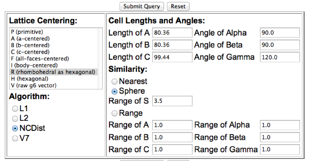
Figure 1: Query box from a SAUC website at http://www.bernstein-plus-sons.com/software/sauc/

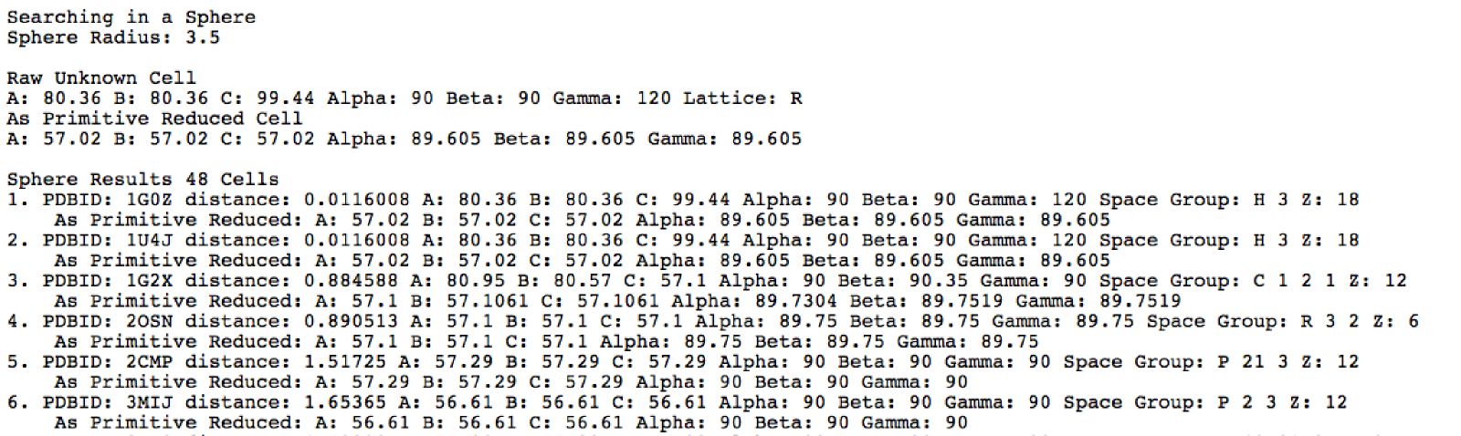
Figure 2: Partial results from SAUC website query

References

- Allen et al. [1973] F. H. Allen, O. Kennard, W. D. S. Motherwell, W. G. Town, and D. G. Watson. Cambridge crystallographic data centre. ii. structural data file. Journal of Chemical Documentation, 13(3):119–123, 1973.
- Andrews [2001] L. Andrews. A template for the nearest neighbor problem. C/C++ Users Journal, 19:40 – 49, 2001. http://sf.net/projects/neartree.