Abstract

A precise evaluation of the two-loop vacuum energy is provided for certain ${\bf Z}_{2}\times{\bf Z}_{2}$ Calabi-Yau orbifold models in the Heterotic string. The evaluation is based on the recent general prescription for superstring perturbation theory in terms of integration over cycles in supermoduli space, implemented at two-loops with the gauge-fixing methods based on the natural projection of supermoduli space onto moduli space using the super-period matrix. It is shown that the contribution from the interior of supermoduli space (computed with the procedure that has been used in previous two-loop computations) vanishes identically for both the $E_{8}\times E_{8}$ and $Spin(32)/{\bf Z}_{2}$ Heterotic strings. The contribution from the boundary of supermoduli space is also evaluated, and shown to vanish for the $E_{8}\times E_{8}$ string but not for the $Spin(32)/{\bf Z}_{2}$ string, thus breaking supersymmetry in this last model. As a byproduct, the vacuum energy in Type II superstrings is shown to vanish as well for these orbifolds.

1 Introduction

In theories with unbroken supersymmetry the vacuum energy vanishes since contributions from bosons and fermions cancel one another identically. When supersymmetry is broken, the masses of bosons and fermions are split and a non-zero net vacuum energy should be produced. It remains a major challenge to achieve mass splittings large enough to fit the Standard Model, accompanied by the production of a vacuum energy small enough to fit present cosmological data.

In superstring theory, mass splittings and vacuum energy should be calculable from first principles. Of special interest are compactifications of Heterotic strings to 4 space-time dimensions in which ${\cal N}=1$ supersymmetry is preserved at string tree-level. A large class of such 6-dimensional compactifications can be constructed using the embedding of the spin connection into the gauge group to guarantee anomaly cancellation [2]. These compactifications include Calabi-Yau manifolds in the large volume limit, and Calabi-Yau orbifolds of flat tori as vacuum solutions to string theory [3].

Non-renormalization theorems restrict the ways in which space-time supersymmetry can be broken by string loop corrections to the appearance of a Fayet-Iliopoulos $D$-term [4]. The Fayet-Iliopoulos (FI) mechanism [5] exists only when the unbroken gauge group contains a commuting $U(1)$-factor, in which case the $D$-term is properly gauge invariant. The standard embeddings of the spin connection into the gauge group distinguish the fate of supersymmetry breaking in the two Heterotic string theories, since we have,

$$Spin(32)/{\bf Z}_{2} \to SU(3)\times U(1)\times SO(26)$$

$$E_{8}~{}\times~{}E_{8} \to SU(3)\times~{}E_{6}~{}\times~{}E_{8}$$ (1.1)

With gauge group $E_{8}\times E_{8}$, no commuting $U(1)$ factor remains, no $D$-term can be generated, and supersymmetry remains unbroken by loop corrections. With gauge group $Spin(32)/{\bf Z}_{2}$, a commuting $U(1)$ factor remains, the FI mechanism is operative, and supersymmetry will be broken by loop corrections. One-loop corrections to the $D$-term tadpole and to the masses of scalars (massless at tree-level) were evaluated in [6, 7] and found to be non-zero. One-loop corrections to the vacuum energy, however, vanish for either case, as contributions arise solely from the tree-level spectra of the theories, which are supersymmetric in both cases. Two loops is the lowest order for which the vacuum energy is sensitive to perturbative supersymmetry breaking in theories with tree-level supersymmetry [8].

Two loops is also the lowest order of superstring perturbation theory for which odd moduli start playing a non-trivial role [9], and where the global structure of supermoduli space must be taken into account when pairing left and right chiral amplitudes [12]. Witten’s prescription for effecting this pairing in the case of Heterotic strings on a genus $h\geq 2$ worldsheet may be briefly summarized as follows. Left chiral amplitudes depend on a supermoduli space $\mathfrak{M}_{h}$ of dimensions $(3-3|2h-2)$, while right chiral amplitudes depend on a bosonic moduli space ${\cal M}_{hR}$ of dimension $(3h-3|0)$. The pairing of left with right chiral amplitudes is realized by integrating their product over a cycle $\Gamma\subset\mathfrak{M}_{h}\times{\cal M}_{hR}$ of dimension $(3h-3|2h-2)$, subject to certain conditions at the Deligne-Mumford compactification divisor. For genus $h\geq 5$, no holomorphic projection $\mathfrak{M}_{h}\to{\cal M}_{h}$ exists [10], and no natural choice of $\Gamma$ is available, but a superspace generalization of Stokes’s theorem [11, 12], guarantees that the full amplitude is independent of the choice of $\Gamma$. As explained in [12], supersymmetric Ward identities have to be realized by integrals of closed forms over supermoduli space.

At two loops, however, there does exist a natural holomorphic projection of the interior of supermoduli space $\mathfrak{M}_{2}$ onto the interior of moduli space ${\cal M}_{2}$ (more precisely onto spin moduli space ${\cal M}_{2,{\rm spin}}$ for even spin structures). This projection may be realized concretely in terms of the genus 2 super-period matrix $\hat{\Omega}$, whose components may be used as locally supersymmetric even moduli. Odd moduli may then be naturally integrated out while keeping $\hat{\Omega}$ fixed. The super-period matrix prescription was used for Type II and Heterotic theories in flat Minkowski space-time, where space-time supersymmetry is unbroken, to compute the superstring measure for even spin structures [13] (see [14] for a survey). In turn, the measure was used to evaluate scattering amplitudes of up to four massless NS bosons, and to prove various non-renormalization theorems [15].

However, subtleties arise, even at genus 2, as one considers extending the natural projection via the super-period matrix, and the pairing of left and right chiralities, to the Deligne-Mumford compactification divisor of supermoduli space $\mathfrak{M}_{2}$ (often referred to as the boundary of supermoduli space). In particular, even if a natural holomorphic projection exists, it does not necessarily lead to a natural cycle $\Gamma$ that behaves as one would like at infinity [16]. These subtleties appear to be inconsequential in background space-times with unbroken supersymmetry, when the string spectrum is sufficiently simple (see section 3.2.5 of [16]). But they do have physical implications, for example, when supersymmetry is broken. In particular, it was conjectured in [16] that the two-loop contribution to the vacuum energy from the interior (or bulk) of supermoduli space vanishes for both Heterotic $Spin(32)/{\bf Z}_{2}$ and $E_{8}\times E_{8}$ theories for any compactification that preserves space-time supersymmetry at tree level. The totality of the two-loop vacuum energy then arises from the boundary of supermoduli space which was shown in [16] to be given by ${\cal V}_{G}=2\pi g_{s}^{2}\langle V_{D}\rangle^{2}$, where $\langle V_{D}\rangle$ is the $D$-term tadpole vacuum expectation value, and $g_{s}$ the string coupling.

In the present paper, we shall compute these two-loop contributions from first principles, both from the interior, as well as from the boundary of supermoduli space, for the special case of $G={\bf Z}_{2}\times{\bf Z}_{2}$ Calabi-Yau orbifolds. These orbifolds are constructed so that the holonomy group $G$ of the spin connection is a subgroup of $SU(3)$, and space-time supersymmetry is preserved at tree level.

We discuss now the contents of the present paper in somewhat greater detail. The models under consideration are orbifolds of $3$-dimensional complex tori, parametrized by complex coordinates $z^{\gamma}$ with $\gamma=1,2,3$. Each non-trivial element of the orbifold group $G$ acts by a ${\bf Z}_{2}$ twist of two of the coordinates $z^{\gamma}$, leaving the third coordinate untwisted, and with corresponding twists also on the RNS worldsheet fermions.

We consider genus 2 worldsheets $\Sigma$ with a fixed homology basis, $A_{I},B_{I}$, satisfying canonical intersection pairing $\#(A_{I}\cap A_{J})=\#(B_{I}\cap B_{J})=0$, $\#(A_{I}\cap B_{J})=\delta_{IJ}$ for $I,J=1,2$. Each ${\bf Z}_{2}$ twist of a field $z^{\gamma}$ gives rise to $2^{4}$ sectors, collectively indexed by a half-characteristic $e^{\gamma}$ for $\gamma=1,2,3$. Thus the twist sectors of the $G$ orbifold theory with all three fields $z^{\gamma}$ may be indexed by vectors $\mathfrak{e}=(e^{1},e^{2},e^{3})$ of three half-characteristics, satisfying the condition,

$$e^{1}+e^{2}+e^{3}=0\quad(\rm mod\ 1)$$ (1.2)

required by the group relations in $G$. The sectors arrange into 6 irreducible orbits under the action of the modular group $Sp(4,{\bf Z})$ on the twists. The key novel orbit, which distinguishes the ${\bf Z}_{2}\times{\bf Z}_{2}$ model from ${\bf Z}_{2}$ models as well as the two-loop order from the one-loop order, is the orbit ${\cal O}_{+}$ to be defined in (2.14).

Our starting point is the gauge-fixed measure on supermoduli space obtained for general superstring compactifications in [17], and worked out explicitly for ${\bf Z}_{2}$ orbifold compactifications in [18]. The left chiral measure arises as a superfield in the odd moduli $\zeta^{1},\zeta^{2}$,

$$d{\cal A}_{L}[\delta;\mathfrak{e}](p_{L\mathfrak{e}};\hat{\Omega},\zeta)=\bigg{(}d\mu^{(0)}_{L}[\delta;\mathfrak{e}](p_{L\mathfrak{e}};\hat{\Omega})+\zeta^{1}\zeta^{2}d\mu_{L}[\delta;\mathfrak{e}](p_{L\mathfrak{e}};\hat{\Omega})\bigg{)}d\zeta^{1}d\zeta^{2}$$ (1.3)

where $\delta$ denotes an even spin structure on the worldsheet, and $p_{L\mathfrak{e}}$ refers to the internal loop momenta. For the Heterotic strings, the right chiral measure depends on internal loop momenta $p_{R\mathfrak{e}}$, on even moduli $\Omega_{R}$, but there are no right odd moduli.

As explained in [16], the bulk contribution to the vacuum energy arises from the top component $d\mu_{L}[\delta;\mathfrak{e}](p_{L\mathfrak{e}};\hat{\Omega})$ of the superfield, while the boundary contribution arises from a regularized limit to the boundary of supermoduli space of the bottom component $d\mu^{(0)}_{L}[\delta;\mathfrak{e}](p_{L\mathfrak{e}},\hat{\Omega})$, paired suitably with the contributions of the right sector. In both cases, the main difficulty will be to determine the contributions from twists $\mathfrak{e}$ in the above-mentioned orbit ${\cal O}_{+}$.

A first main result of this paper is the vanishing, pointwise on supermoduli space, of the bulk contribution from each twist in the orbit ${\cal O}_{+}$, upon summing over the spin structures $\delta$, as required for the GSO projection. An essential ingredient in this vanishing is the subtle correction term $\Gamma[\delta;\varepsilon]$ uncovered in [18], which distinguishes between the Prym period matrix of the super Riemann surface, and the supersymmetric covariance matrix arising from the chiral splitting of the super matter fields. Taking this correction term into account, the bulk contribution for sectors in ${\cal O}_{+}$ can then be shown to vanish by a seemingly new identity (6.1) between $\vartheta$-constants. Mathematically, this identity is more subtle than other more familiar identities, since it is only covariant with respect to a coset subgroup $Sp(4,{\bf Z})/{\bf Z}_{4}$ rather than the full modular group $Sp(4,{\bf Z})$. Thus the identity cannot be established just from standard structure theorems for the ring of genus 2 modular forms and examining its behavior in the degeneration limit. It should be an interesting mathematical problem to develop structure theorems for genus 2 modular forms with respect to natural modular subgroups such as $Sp(4,{\bf Z})/{\bf Z}_{4}$, and use such theorems to understand identities of the type proven in (6.1).

The second main result of the paper is the evaluation of the boundary contributions to the vacuum energy. Following the prescription of [16], the left and right sectors are paired together not by setting $\hat{\Omega}=\Omega_{R}$ as would be done for the bulk contribution, but rather by a nilpotent regularization of the conditionally convergent integrals that arise at the separating degenerating node. With this prescription, the contributions of twists in each orbit can be calculated using degeneration formulas for $\vartheta$-functions and some simplifications derived from earlier work in [19]. In the approach of [17], the bottom component of the chiral measure has an intermediate dependence on the choice of slice in the gauge-fixing procedure. With the help of the regularization of [16] near the separating node, proper gauge slice independence is restored for the full boundary contribution.

With this preparation, we find then that the boundary contributions to the vacuum energy vanish in all models for all twists not belonging to ${\cal O}_{+}$. But for twists in ${\cal O}_{+}$, the structure of the GSO summation over right spin structures $\delta_{R}$ of the internal fermion partition function factors $\overline{\vartheta[\delta_{R}]}^{4\mathfrak{n}}$ in the right sector differs for the two Heterotic theories. Since for the $E_{8}\times E_{8}$ string we have $\mathfrak{n}=1$, while for the $Spin(32)/{\bf Z}_{2}$ string we have $\mathfrak{n}=3$, we will find that the vacuum energy contribution vanishes for the $E_{8}\times E_{8}$ string, while it is strictly positive for the $Spin(32)/{\bf Z}_{2}$ string. Its value in the latter case will be evaluated explicitly.

As a byproduct, we confirm that contributions from the interior and from the boundary of supermoduli space vanish for Type II strings compactified on the same ${\bf Z}_{2}\times{\bf Z}_{2}$ Calabi-Yau orbifolds.

1.1 Organization

The paper is organized as follows. In Section 2, we describe the ${\bf Z}_{2}\times{\bf Z}_{2}$ Calabi-Yau orbifold model, the indexing of the orbifold sectors by vectors $\mathfrak{e}$ of twists, and the orbit structure of the vectors $\mathfrak{e}$ under the modular group. In Section 3, we calculate the partition function for each fixed spin structure. This begins with a description of the results of [18] for $d{\cal A}_{L}[\delta;\mathfrak{e}]$, together with a description of the contributions of the matter fields, whether they are compactified, twisted, or a combination of both. The matter fields contributions are then worked out orbit by orbit. The section concludes with the explicit evaluation of the contributions of the right sector for both $E_{8}\times E_{8}$ and $Spin(32)/{\bf Z}_{2}$ Heterotic theories, which is straightforward. Sections 4 and 5 are devoted to the identification of the GSO phases and the summation over spin structures, for sectors in the orbits distinct from ${\cal O}_{+}$ and sectors in ${\cal O}_{+}$ respectively. For sectors in all orbits distinct from ${\cal O}_{+}$, the contributions are found to vanish by the $\vartheta$-function identities already established in [17] and [18]. The contribution of sectors from the orbit ${\cal O}_{+}$ is found to vanish by the new identity (6.1), the proof of which is the subject of Section 6. Sections 7 and 8 are devoted to the evaluation of the boundary contributions, again for sectors in the orbits distinct from ${\cal O}_{+}$ and sectors in ${\cal O}_{+}$ respectively. The former all vanish by genus $1$ Riemann identities, while the latter exhibits the different behavior explained above for the both $E_{8}\times E_{8}$ and $Spin(32)/{\bf Z}_{2}$ Heterotic strings.

Some useful items have been gathered in the appendices for the convenience of the reader. Basic formulas for genus one $\vartheta$-functions are listed in Appendix A. Appendix B contains similar formulas for genus two $\vartheta$-functions, together with a detailed account of modular transformations acting on characteristics. In Appendix C, a new and simplified evaluation of the sign factor for the term $\Gamma[\delta;\varepsilon]$ is provided in detail. This factor was not given correctly in [18]; it ended up being immaterial there, but will play a crucial role in the present paper.

Acknowledgments

We are very grateful to Edward Witten for suggesting the orbifold problem to us, for sharing his paper [16] with us prior to publication, and for detailed and very helpful comments all along the project as well as on a draft of this paper. One of us (E.D.) is happy to acknowledge the generous hospitality of the Columbia University Department of Mathematics, where part of this work was completed.

2 ${\bf Z}_{2}\times{\bf Z}_{2}$ Calabi-Yau Orbifold Compactifications

We shall consider Heterotic and Type II superstring theories compactified on 6-dimensional ${\bf Z}_{2}\times{\bf Z}_{2}$ Calabi-Yau orbifolds, as described for example in [20, 21]. Ten-dimensional space-time is of the form $M_{4}\times Y$ where $M_{4}$ is 4-dimensional Minkowski space-time and the internal space $Y$ is an orbifold of a 6-dimensional torus,

$$Y=(T_{1}\times T_{2}\times T_{3})/G.$$ (2.1)

The orbifold group $G$ is isomorphic to ${\bf Z}_{2}\times{\bf Z}_{2}$. The complex tori $T_{\gamma}$ are given by $T_{\gamma}={\bf C}/\Lambda_{\gamma}$ for $\gamma=1,2,3$, where the lattices $\Lambda_{\gamma}$ are defined by,

$$\Lambda_{\gamma}=\{m_{\gamma}+n_{\gamma}t_{\gamma}~{}\hbox{with}~{}m_{\gamma},n_{\gamma}\in{\bf Z}\}$$ (2.2)

for some fixed moduli $t_{\gamma}\in{\bf C}$ with ${\rm Im\,}t_{\gamma}>0$. Setting $\Lambda=\Lambda_{1}\times\Lambda_{2}\times\Lambda_{3}$, we may also view the torus as $T_{1}\times T_{2}\times T_{3}={\bf C}^{3}/\Lambda$, and use local complex coordinates $(z^{1},z^{2},z^{3})$.

For the Heterotic strings with either gauge group $Spin(32)/Z_{2}$ or $E_{8}\times E_{8}$, the orbifold group $G={\bf Z}_{2}\times{\bf Z}_{2}$ is chosen to be a subgroup of the $SU(3)\subset SO(6)$ acting on $T_{1}\times T_{2}\times T_{3}$. Thus, $Y$ is a Calabi-Yau orbifold and ${\cal N}=1$ supersymmetry is preserved in the effective 4-dimensional theory. The holonomy group of the spin connection is embedded into the gauge group to assure proper anomaly cancellation. For Type II superstrings, compactification on the orbifold $Y$ will preserve ${\cal N}=2$ supersymmetry in the effective 4-dimensional theory.

2.1 Fields

The worldsheet fields in the RNS formulation will be denoted as follows. Bosonic fields for Minkowski $M_{4}$ are real and denoted by $x^{\mu}$ with $\mu=0,1,2,3$, while those for the internal space $Y$ are complex fields $z^{\gamma},z^{\bar{\gamma}}$ with $\gamma,\bar{\gamma}=1,2,3$. The left chirality fermionic fields are similarly split into $\psi_{+}^{\mu}$ and $\psi^{\gamma},\psi^{\bar{\gamma}}$. For the Type II strings, the right chirality fermions are split into $\psi_{-}^{\mu}$ and $\tilde{\psi}^{\gamma},\tilde{\psi}^{\bar{\gamma}}$. For Heterotic strings, we shall use the fermionic representation of the internal degrees of freedom in terms of 32 right chirality fermions $\psi_{-}^{A}$ with $A=1,\cdots,32$. Upon embedding the spin connection with holonomy group $G\subset SU(3)$ into the gauge group, we split also these fermions in a manner natural to this $SU(3)$ action, into $\psi_{-}^{\alpha}$ with $\alpha=1,\cdots,26$ and $\xi^{\gamma},\xi^{\bar{\gamma}}$ with $\gamma,\bar{\gamma}=1,2,3$. In summary, the fields $z^{\gamma},\psi^{\gamma},\xi^{\gamma}$ transform under a ${\bf 3}$ of $SU(3)$ while $z^{\bar{\gamma}},\psi^{\bar{\gamma}},\xi^{\bar{\gamma}}$ transform under the $\bar{\bf 3}$.

For gauge group $Spin(32)/{\bf Z}_{2}$, an additional commuting $U(1)$ factor arises in the embedding $SU(3)\times U(1)\subset SO(6)\subset SO(32)$ under which the fields $\psi^{\gamma}$ and $\xi^{\gamma}$ have charge 1, while $\psi^{\bar{\gamma}}$ and $\xi^{\bar{\gamma}}$ have charge $-1$ for all $\gamma,\bar{\gamma}=1,2,3$. The associated conserved $U(1)$ current is given by (repeated indices are summed), $J_{z}=\delta_{\gamma\bar{\gamma}}\,\psi^{\gamma}\psi^{\bar{\gamma}}$ and $J_{\bar{z}}=\delta_{\gamma\bar{\gamma}}\,\xi^{\gamma}\xi^{\bar{\gamma}}$.

The spin structure assignments in this orbifold model are as follows. The left chirality fermions $\psi^{\mu}_{+}$ and $\psi^{\gamma},\psi^{\bar{\gamma}}$ couple to the worldsheet gravitino field, so they all must have the same spin structure, which we denote by $\delta$. For the $Spin(32)/{\bf Z}_{2}$ string, all 32 internal fermions $\psi_{-}^{\alpha},\xi^{\gamma},\xi^{\bar{\gamma}}$ have common spin structure $\delta_{R}$, which is summed over to carry out the GSO projection and guarantee modular invariance. For the $E_{8}\times E_{8}$ string, the 32 fermions are grouped into two sets of 16 fermions each. Within each set, the 16 fermions are assigned the same spin structure, $\delta_{R}^{1}$ for the first set, and $\delta_{R}^{2}$ for the second set. The summation over spin structures is performed over all $\delta_{R}^{1}$ and $\delta_{R}^{2}$, independently of each other.

As was explained in the Introduction, the orbifold compactification breaks the gauge symmetries of the Heterotic strings in different fashions. For the $Spin(32)/{\bf Z}_{2}$ string, the gauge symmetry is broken to,

$$Spin(32)/{\bf Z}_{2}\to SU(3)\times U(1)\times SO(26)\to U(1)\times SO(26)$$ (2.3)

For the $E_{8}\times E_{8}$ string, the embedding of $G\subset SU(3)$ will be restricted to only one of the $E_{8}$ factors, so that the twisted fermions $\xi^{\gamma},\xi^{\bar{\gamma}}$ with $\gamma,\bar{\gamma}=1,2,3$ belong to the first group of 16 right fermions. With this assignment, the gauge symmetry is broken to,

$$E_{8}\times E_{8}\to SU(3)\times E_{6}\times E_{8}\to E_{6}\times E_{8}$$ (2.4)

In both theories, the $SU(3)$ itself is broken by the spin connection when the orbifold group is $G={\bf Z}_{2}\times{\bf Z}_{2}$. (When the orbifold group is the center $G={\bf Z}_{3}$ of $SU(3)$, however, an unbroken $SU(3)$ will remain as well; this was the situation analyzed in [6, 7].)

2.2 Action of the orbifold group on the fields

The action of the group $G=\{1,\lambda_{1},\lambda_{2},\lambda_{3}\}$ on $z^{\gamma}$, $\psi^{\gamma}$, and $\xi^{\gamma}$ for $\gamma=1,2,3$ is given by,

$$\lambda_{\beta}\,z^{\gamma} = (2\delta_{\beta,\gamma}-1)z^{\gamma}$$

$$\lambda_{\beta}\,\psi^{\gamma} = (2\delta_{\beta,\gamma}-1)\psi^{\gamma}$$

$$\lambda_{\beta}\,\xi^{\gamma} = (2\delta_{\beta,\gamma}-1)\xi^{\gamma}$$ (2.5)

and similarly for the fields $z^{\bar{\gamma}},\psi^{\bar{\gamma}}$ and $\xi^{\bar{\gamma}}$. The remaining fields, $x^{\mu}$, $\psi^{\mu}_{+}$ for $\mu=0,1,2,3$ and $\psi_{-}^{\alpha}$ for $\alpha=1,\cdots,26$ are invariant under $G$.

2.3 Twisted sectors in terms of characteristics

In the previous section, we have described the action of the orbifold group $G$ on the fields. We now identify all the twisted sectors which arise in the orbifold theory, and we express each twist sector in terms of a vector $\mathfrak{e}$ of three characteristics $\mathfrak{e}=(e^{1},e^{2},e^{3})$.

Figure 1: Canonical homology basis for genus 2.

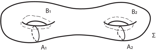
We choose a basis of homology cycles $A_{I},B_{I}$ in $H^{1}(\Sigma,{\bf Z})$ with canonical normalization $\#(A_{I},A_{J})=\#(B_{I},B_{J})=0$ and $\#(A_{I},B_{J})=\delta_{IJ}$, as shown in Figure 1. For each value of $\gamma=\bar{\gamma}=1,2,3$, the fields $z^{\gamma},z^{\bar{\gamma}},\psi^{\gamma},\psi^{\bar{\gamma}}$ and $\xi^{\gamma},\xi^{\bar{\gamma}}$ are twisted in the same manner by a single ${\bf Z}_{2}$ twist. We shall label this twist by a genus 2 half-characteristic $e^{\gamma}$ using the standard notation with $(e^{\gamma})^{\prime}_{I},(e^{\gamma})^{\prime\prime}_{I}\in\{0,{1\over 2}\}$ for $I=1,2$,

$$e^{\gamma}=\left(\matrix{(e^{\gamma})^{\prime}_{1}\cr(e^{\gamma})^{\prime}_{2}\cr}\bigg{|}\matrix{(e^{\gamma})^{\prime\prime}_{1}\cr(e^{\gamma})^{\prime\prime}_{2}\cr}\right)$$ (2.6)

Similarly, we label the spin structures $\delta$ and $\delta_{R}$ by half-characteristics $\delta=(\delta_{I}^{\prime}|\delta_{I}^{\prime\prime})$ and $\delta_{R}=((\delta_{R})_{I}^{\prime}|(\delta_{R})_{I}^{\prime\prime})$ respectively. Taking into account the spin structure assignments of the fermion fields, the monodromy relations are as follows. Around $A_{I}$-cycles we have,

$$z^{\gamma}(w+A_{I}) = (-)^{2(e^{\gamma})^{\prime}_{I}}z^{\gamma}(w)$$

$$\psi^{\gamma}(w+A_{I}) = (-)^{2(e^{\gamma})^{\prime}_{I}+2\delta_{I}^{\prime}}\,\psi^{\gamma}(w)$$

$$\xi^{\gamma}(w+A_{I}) = (-)^{2(e^{\gamma})^{\prime}_{I}+2(\delta_{R})_{I}^{\prime}}\,\xi^{\gamma}(w)$$ (2.7)

and for $B_{I}$-cycles,

$$z^{\gamma}(w+B_{I}) = (-)^{2(e^{\gamma})^{\prime\prime}_{I}}z^{\gamma}(w)$$

$$\psi^{\gamma}(w+B_{I}) = (-)^{2(e^{\gamma})^{\prime\prime}_{I}+2\delta_{I}^{\prime\prime}}\,\psi^{\gamma}(w)$$

$$\xi^{\gamma}(w+B_{I}) = (-)^{2(e^{\gamma})^{\prime\prime}_{I}+2(\delta_{R})_{I}^{\prime\prime}}\,\xi^{\gamma}(w)$$ (2.8)

The combined twist $\mathfrak{e}=(e^{1},e^{2},e^{3})$ of all compactified fields, $z^{\gamma},z^{\bar{\gamma}},\psi^{\gamma},\psi^{\bar{\gamma}},\xi^{\gamma},\xi^{\bar{\gamma}}$ for $\gamma=1,2,3$, represents a group element of $G={\bf Z}_{2}\times{\bf Z}_{2}$ provided we have the relation,

$$e^{1}+e^{2}+e^{3}\equiv 0\qquad(\hbox{mod}~{}1)$$ (2.9)

and all twists by $G$ may be implemented uniquely on $\Sigma$ in this manner.

A different, but equivalent, way of implementing the representation of $G$ on the fields is by working with the two group factors of $G={\bf Z}_{2}\times{\bf Z}_{2}$ separately. Let $\lambda_{1}$ and $\lambda_{2}$ generate the first and second ${\bf Z}_{2}$ factors respectively. All possible twist sectors may be labelled by the cycles $D_{\eta}$ and $D_{\varepsilon}$ in $H^{1}(\Sigma,Z_{2})$ around which the twisting by $\lambda_{1}$ and $\lambda_{2}$ is carried out. Each cycle $D_{\varepsilon}$ (resp. $D_{\eta}$) may be represented in terms of a half-integer characteristic $\varepsilon$ (resp. $\eta$),

$$D_{\varepsilon}=\sum_{I}\left(2\varepsilon^{\prime}_{I}A_{I}+2\varepsilon^{\prime\prime}_{I}B_{I}\right)$$ (2.10)

The action of the element $\lambda_{3}$ is now fixed, since it is already realized as the product $\lambda_{3}=\lambda_{1}\lambda_{2}$. This representation coincides with the one given in (2.3) and (2.3), provided we identify,

$$\mathfrak{e}=(e^{1},e^{2},e^{3})=(\varepsilon,\eta,\varepsilon+\eta)\qquad(\hbox{mod}~{}1)$$ (2.11)

a realization which automatically satisfies the condition (2.9).

2.4 Modular orbits of the twists

The modular transformation properties of a single twist $\varepsilon$ are listed in Appendix B. To summarize: of the 16 twists, one is invariant under modular transformations (corresponding to no twisting), while the remaining 15 transform in a single irreducible modular orbit, which we denote by ${\cal E}$. The subgroup $H_{\varepsilon}\subset Sp(4,{\bf Z})$ which leaves a non-zero twist $\varepsilon$ invariant may be determined for any convenient twist, for example $\varepsilon=\varepsilon_{2}$. By inspection of table 4), we see that the group $H_{\varepsilon_{2}}$ is generated by the elements $M_{1},M_{2},M_{3},T_{2}=\Sigma T\Sigma$, and $S_{2}=SM_{1}SM_{1}$, where $M_{1},M_{2},M_{3},S,T,\Sigma$ are defined in (B.13). The groups $H_{\varepsilon}$ for general $\varepsilon$ may be obtained from $H_{\varepsilon_{2}}$ by conjugation $H_{\varepsilon}=MH_{\varepsilon_{2}}M^{-1}$ by any modular transformation $M$ which maps the reference twist $\varepsilon_{2}$ to the general twist $\varepsilon=M\varepsilon_{2}$.

We denote by ${\cal O}_{\rm tot}$ the set of all possible twisted sectors of our full orbifold theory. Following the description of the previous section, ${\cal O}_{\rm tot}$ may be identified with the set of all triplets of half characteristics $\mathfrak{e}=(e^{1},e^{2},e^{3})$ with $e^{1}+e^{2}+e^{3}\equiv 0$ (mod 1). The orbifold quantum field theory requires a summation over all sectors, and thus over all triplets of twists $\mathfrak{e}$. It will be convenient to organize this summation in terms of orbits which are irreducible under the action of the modular group $Sp(4,{\bf Z})$. To do so, it will be convenient to parametrize $\mathfrak{e}=(\varepsilon,\eta,\varepsilon+\eta)$ by a pair $(\varepsilon,\eta)$ of independent twists, as was explained in the preceding section. The set of all pairs of twists $(\varepsilon,\eta)$ may be distinguished by their transformation properties, and arranged into the following cases.

1. $\varepsilon=\eta=0$ gives the untwisted sector;

2. $\varepsilon=0$ and $\eta\not=0$ is the sector twisted by $\lambda_{1}$;

3. $\eta=0$ and $\varepsilon\not=0$ is the sector twisted by $\lambda_{2}$;

4. $\eta=\varepsilon$ and $\varepsilon\not=0$ is the sector twisted by $\lambda_{3}$;

5. $0\not=\varepsilon\not=\eta\not=0$.

We readily deduce the decomposition of ${\cal O}_{\rm tot}$ into irreducible modular orbits.

$\bullet$ Case 0. above corresponds to the orbit ${\cal O}_{0}$ with a single point, the zero twist,

$${\cal O}_{0}=\{(\varepsilon,\eta),~{}\varepsilon=\eta=0\}$$ (2.12)

This is the untwisted sector, and it is invariant under the full modular group $Sp(4,{\bf Z})$.

$\bullet$ Cases 1. 2. and 3. correspond to the irreducible orbits of a single ${\bf Z}_{2}$ subgroup of $G$. Each case is isomorphic to the non-zero irreducible orbit ${\cal E}$ of a single twist, and we have,

$${\cal O}_{1} = \{\mathfrak{e}=(0,\varepsilon,\varepsilon),~{}\varepsilon\in{\cal E}\}$$

$${\cal O}_{2} = \{\mathfrak{e}=(\varepsilon,0,\varepsilon),~{}\varepsilon\in{\cal E}\}$$

$${\cal O}_{3} = \{\mathfrak{e}=(\varepsilon,\varepsilon,0),~{}\varepsilon\in{\cal E}\}$$ (2.13)

$\bullet$ Case 4. above comprises two irreducible modular orbits ${\cal O}_{\pm}$, distinguished as follows,

$${\cal O}_{\pm}=\{\mathfrak{e}=(\varepsilon,\eta,\varepsilon+\eta),~{}\varepsilon,\eta\in{\cal E},~{}\varepsilon\not=\eta,~{}\langle\varepsilon|\eta\rangle=\pm 1\}$$ (2.14)

where $\langle\varepsilon|\eta\rangle$ is the standard mod 2 symplectic invariant, which takes the form,

$$\langle\varepsilon|\eta\rangle=\exp\{4\pi i(\varepsilon^{\prime}\cdot\eta^{\prime\prime}-\eta^{\prime}\cdot\varepsilon^{\prime\prime})\}$$ (2.15)

The fact that ${\cal O}_{+}$ and ${\cal O}_{-}$ each forms a single irreducible modular orbit may be proven by explicit construction of the orbits. To do so, we again use the fact that for any twist $\varepsilon$ there exists a modular transformation $M$ such that $\varepsilon=M\varepsilon_{2}$. It is now straightforward to distinguish the pairs $(\varepsilon,\eta)$ that belong to ${\cal O}_{\pm}$, and we find,

$${\cal O}_{+} = \left\{\mathfrak{e}=M(\varepsilon_{2},\eta,\varepsilon_{2}+\eta),~{}\eta\in\{\varepsilon_{3},\,\varepsilon_{4},\,\varepsilon_{7},\,\varepsilon_{8},\,\varepsilon_{12},\,\varepsilon_{14}\},~{}M\in Sp(4,{\bf Z})\right\}$$ (2.16)

$${\cal O}_{-} = \left\{\mathfrak{e}=M(\varepsilon_{2},\eta,\varepsilon_{2}+\eta),~{}\eta\in\{\varepsilon_{5},\,\varepsilon_{6},\,\varepsilon_{9},\,\varepsilon_{10},\,\varepsilon_{11},\,\varepsilon_{13},\,\varepsilon_{15},\,\varepsilon_{16}\},~{}M\in Sp(4,{\bf Z})\right\}$$

By applying the subgroup $H_{\varepsilon_{2}}$ respectively to the pairs, $(\varepsilon_{2},\varepsilon_{3})\in{\cal O}_{+}$, and $(\varepsilon_{2},\varepsilon_{5})\in{\cal O}_{-}$, one verifies that each orbit ${\cal O}_{\pm}$ transforms irreducibly under $Sp(4,{\bf Z})$. Note that these two cases have clear geometrical interpretations. Given that $\varepsilon=\varepsilon_{2}$ corresponds to a twist around the cycle $B_{2}$, the case $\eta\in{\cal O}_{+}$ corresponds to a twist around the cycle $B_{1}$ for $\eta=\varepsilon_{3}$, while the case $\eta\in{\cal O}_{-}$ corresponds to a twist around the cycle $A_{2}$ for $\eta=\varepsilon_{5}$.

$\bullet$ The union of all orbits equals ${\cal O}_{{\rm tot}}$. The cardinalities indeed check, using the fact that the cardinalities of ${\cal O}_{0},{\cal O}_{i},{\cal O}_{+},{\cal O}_{-}$ are respectively given by 1, 15 (with multiplicity 3), 90, and 120, adding up to $256=16^{2}$, as expected.

3 The Two-Loop Vacuum Energy

Following [17, 18], the vacuum energy of a superstring compactification is built from the holomorphic blocks of the ghost and super ghost system as in flat space-time, and from the holomorphic blocks of the matter fields of the compactification. For orbifold models, the contributions from the matter fields from all twisted sectors must be included. As shown in Section 2, the sectors are labeled the twists $\mathfrak{e}=(e^{1},e^{2},e^{3})$, so that the sum over all sectors can be viewed as the sum over the set ${\cal O}_{\rm tot}$ of all 256 possible twists $\mathfrak{e}$.

3.1 General structure of the two-loop vacuum energy

Specializing the expressions of [18] (which were written in all generality, so as to include both symmetric and asymmetric orbifold constructions) to the case of the symmetric $G={\bf Z}_{2}\times{\bf Z}_{2}$ orbifolds discussed in Section 2, the vacuum energy ${\cal V}_{G}$ takes the form,

$${\cal V}_{G}=g_{s}^{2}\,\mathfrak{N}\,\int_{\Gamma}\sum_{\mathfrak{e}\,\in{\cal O}_{{\rm tot}}}\sum_{p_{L\mathfrak{e}},p_{R\mathfrak{e}}}C_{\delta}[\mathfrak{e}]\,d{\cal A}_{L}[\delta;\mathfrak{e}](p_{L\mathfrak{e}};\hat{\Omega},\zeta)\wedge\overline{d\mu_{R}[\mathfrak{e}](p_{R\mathfrak{e}};\Omega_{R})}$$ (3.1)

In particular, the pairing factor $K(\mathfrak{e},p_{L\mathfrak{e}},p_{R\mathfrak{e}})$, which was needed for the general formulation of [18], may be set to equal an overall normalization factor $\mathfrak{N}$, multiplied by the coupling $g_{s}^{2}$ for two loops, as was done in (3.1). The notation for the remaining ingredients is as follows:

$\bullet$ The first sum, running over all twists $\mathfrak{e}\in{\cal O}_{\rm tot}$, represents the sum over all sectors of the orbifold theory. In view of the decomposition of ${\cal O}_{\rm tot}$ into modular orbits ${\cal O}_{\alpha}$ in the previous section, the sum over ${\cal O}_{{\rm tot}}$ may be recast in terms of a sum over irreducible orbits,

$$\sum_{\mathfrak{e}\,\in{\cal O}_{\rm tot}}\ =\ \sum_{\alpha}\sum_{\mathfrak{e}\,\in{\cal O}_{\alpha}}$$ (3.2)

with the label $\alpha$ taking values in $\{0,1,2,3,\pm\}$.

$\bullet$ The second sum runs over all left and right momenta $(p_{L\mathfrak{e}},p_{R\mathfrak{e}})$ for fixed twist $\mathfrak{e}$. Note that left and right-momenta are in general different since we compactify on a 6-dimensional torus. We shall describe their range at the end of Section 3.2.

$\bullet$ Following [12] for the Heterotic string, the integration is over an arbitrary cycle $\Gamma\subset\mathfrak{M}_{2}\times{\cal M}_{2R}$ (subject to certain asymptotic and reality conditions). Here ${\cal M}_{2R}$ is the moduli space of all Riemann surfaces of genus $2$ used for right chiral amplitudes, and $\mathfrak{M}_{2}$ is the supermoduli space of all super Riemann surfaces of genus $2$, used for left chiral amplitudes. The independence of the integral on the choice of cycle $\Gamma$ is guaranteed by a super Stokes theorem. The sum over spin structures is an integral part of the integration over $\mathfrak{M}_{2}$ and thus $\Gamma$. For general genus, the summation over spin structures cannot be separated in this process from the integration over odd moduli.

$\bullet$ In genus 2, we have a natural projection from $\mathfrak{M}_{2}$ onto ${\cal M}_{2}$ provided by the super-period matrix [14, 17]. Thus, we may parametrize $\mathfrak{M}_{2}$ by $(\hat{\Omega},\zeta;\delta)$ where $\hat{\Omega}$ is the super-period matrix of the underlying super Riemann surface, $\zeta$ the two odd moduli of genus 2, and $\delta$ the spin structure. The GSO phases $C_{\delta}[\mathfrak{e}]$ are determined so as to guarantee modular invariance of the integrand. After integration over the odd moduli, the spin structures $\delta$ are summed according to the GSO projection. Parametrizing ${\cal M}_{2R}$ by a period matrix $\Omega_{R}$, the choice of the cycle $\Gamma$ corresponds to the choice of a relation between $\hat{\Omega}$ and $\Omega_{R}$. The general form of such relations is dictated by complex conjugation, up to the addition of nilpotent terms bilinear in the odd moduli $\zeta$ [16],

$$\hat{\Omega}=\Omega_{R}+{\cal O}(\zeta^{1}\zeta^{2}).$$ (3.3)

$\bullet$ The bulk contribution of supermoduli space is obtained from the top component of $d{\cal A}_{L}[\delta;\mathfrak{e}]$ in an expansion in the odd moduli $\zeta^{1},\zeta^{2}$. For this contribution, the term ${\cal O}(\zeta^{1}\zeta^{2})$ in (3.3) is immaterial, and the natural choice is to set $\hat{\Omega}=\Omega_{R}$. But, as was shown in [16], for the boundary contribution of supermoduli space a regularization of conditionally convergent integrals may produce a non-vanishing contribution from the bottom component of $d{\cal A}_{L}[\delta;\mathfrak{e}]$, and the term ${\cal O}(\zeta^{1}\zeta^{2})$ does matter. More specifically, if $\hat{\Omega}$ is viewed as the super-period matrix of a supergeometry $(g_{mn},\chi_{\bar{z}}{}^{+})$, and $\Omega$ is the period matrix of the metric $g_{mn}$, then the correct relation (3.3) for the boundary contributions amounts essentially to a regularized version of setting $\Omega=\Omega_{R}$ near the boundary of supermoduli space.

$\bullet$ The left block $d{\cal A}_{L}[\delta;\mathfrak{e}](p_{L\mathfrak{e}};\hat{\Omega},\zeta)$ depends on the left spin structure $\delta$, the super-period matrix $\hat{\Omega}$ and the odd moduli $\zeta$. The right block $d\mu_{R}[\mathfrak{e}](p_{R\mathfrak{e}};\Omega_{R})$ depends on moduli $\Omega_{R}$.

Concretely, we begin by making explicit the dependence on odd moduli $\zeta$,

$$d{\cal A}_{L}[\delta;\mathfrak{e}](p_{L\mathfrak{e}};\hat{\Omega},\zeta)=\bigg{(}d\mu^{(0)}_{L}[\delta;\mathfrak{e}](p_{L\mathfrak{e}},\hat{\Omega})+\zeta^{1}\zeta^{2}d\mu_{L}[\delta;\mathfrak{e}](p_{L\mathfrak{e}};\hat{\Omega})\bigg{)}d\zeta^{1}d\zeta^{2}$$ (3.4)

Carrying out the integration over $\zeta$ will then produce the following contributions,

$${\cal V}_{G}={\cal V}_{G}^{\rm bdy}+{\cal V}_{G}^{\rm bulk}$$ (3.5)

where the term ${\cal V}^{\rm bulk}_{G}$ refers to the contribution from the bulk of supermoduli space, while ${\cal V}_{G}^{\rm bdy}$ refers to the contributions from conditionally convergent integrals arising from the boundary of supermoduli space. The bulk term is the contribution of the top component $d\mu_{L}[\delta;\mathfrak{e}]$ in which we may set $\hat{\Omega}=\Omega_{R}\equiv\Omega$, as was explained earlier. Thus the bulk term is given by,

$${\cal V}_{G}^{\rm bulk}=g_{s}^{2}\mathfrak{N}\,\int_{{\cal M}_{2}}\sum_{\mathfrak{e}\,\in{\cal O}_{{\rm tot}}}\sum_{p_{L\mathfrak{e}},p_{R\mathfrak{e}}}\sum_{\delta}C_{\delta}[\mathfrak{e}]\,d\mu_{L}[\delta;\mathfrak{e}](p_{L\mathfrak{e}};\Omega)\wedge\overline{d\mu_{R}[\mathfrak{e}](p_{R\mathfrak{e}};\Omega)}.$$ (3.6)

The boundary contribution is from the term $d\mu^{(0)}_{L}[\delta;\mathfrak{e}]$ and will be schematically denoted by,

$${\cal V}_{G}^{\rm bdy}=g_{s}^{2}\mathfrak{N}\,\int_{\partial\Gamma}\sum_{\mathfrak{e}\,\in{\cal O}_{{\rm tot}}}\,\sum_{p_{L\mathfrak{e}},p_{R\mathfrak{e}}}\,C_{\delta}[\mathfrak{e}]\,d\mu^{(0)}_{L}[\delta;\mathfrak{e}](p_{L\mathfrak{e}};\hat{\Omega})d\zeta^{1}d\zeta^{2}\wedge\overline{d\mu_{R}[\mathfrak{e}](p_{R\mathfrak{e}};\Omega_{R})}$$ (3.7)

with the understanding that the regularization procedure of [12] must be used to parametrize and relate $\hat{\Omega},\zeta$, and $\Omega_{R}$ at the boundary $\partial\Gamma$ of the cycle $\Gamma$. It will be seen that, with the proper choice of cycle $\Gamma$ and after the regularization procedure, the term ${\cal V}_{G}^{\rm bdy}$ reduces to an integral over the separating node divisor part of the boundary of moduli space.

3.2 Internal loop momenta

The range of the internal loop momenta $(p_{L\mathfrak{e}},p_{R\mathfrak{e}})$ depends on whether the corresponding fields are uncompactified, compactified but untwisted, or compactified with a non-zero twist.

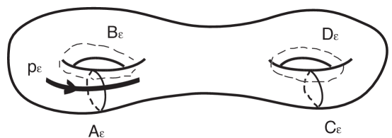
For each value of $\gamma=1,2,3$, the fields $z^{\gamma},z^{\bar{\gamma}},\psi^{\gamma},\psi^{\bar{\gamma}},\xi^{\gamma},\xi^{\bar{\gamma}}$ are untwisted when $e^{\gamma}=0$, and twisted by a common ${\bf Z}_{2}$ when $e^{\gamma}\not=0$. A field subject to a ${\bf Z}_{2}$ twist $\varepsilon=e^{\gamma}$ may be viewed as defined on the surface $\Sigma$ with a quadratic branch cut along a cycle $C_{\varepsilon}$, as represented in Figure 2. The ${\bf Z}_{2}$-twisted field is then double-valued around the conjugate cycle $D_{\varepsilon}$, defined earlier in (2.10). The remaining two cycles $A_{\varepsilon},B_{\varepsilon}$ are defined so that $\#(A_{\varepsilon},B_{\varepsilon})=\#(C_{\varepsilon},D_{\varepsilon})=1$ with all other intersection numbers vanishing.

Figure 2: Canonical cycles and internal loop momenta $p_{\varepsilon}=(p_{\varepsilon}^{\gamma},p_{\varepsilon}^{\bar{\gamma}})$ for twist $\varepsilon=e^{\gamma}\not=0$.

$\bullet$ In the uncompactified dimensions, $\mu=0,1,2,3$, left and right internal loop momenta are equal, and denoted by $p^{\mu}_{I}$. They may be viewed as traversing cycles $A_{I}$ in Figure 1.

$\bullet$ In the compactified dimensions, we distinguish twisted from untwisted directions (this distinction will depend on the modular orbit of the twist). For the untwisted fields $z^{\gamma},z^{\bar{\gamma}}$, we have internal loop momenta $(p^{\gamma}_{LI},p^{\bar{\gamma}}_{LI})$ and $(p^{\gamma}_{RI},p^{\bar{\gamma}}_{RI})$ with $I=1,2$, which may be viewed as traversing cycles $A_{I}$ in Figure 1. They correspond to the torus compactification, and may be parametrized by the lattice $\Lambda$ of (2.2), and its dual $\Lambda^{*}$. The result is standard [22],

$$p_{LI}=k_{I}-{1\over 2}\ell_{I}\hskip 72.26999ptp_{RI}=k_{I}+{1\over 2}\ell_{I}$$ (3.8)

with the vectors $k_{I}\in\Lambda^{*}$ and $\ell_{I}\in\Lambda$ for $I=1,2$, in units where $\alpha^{\prime}=2$.

$\bullet$ For the twisted fields $z^{\gamma},z^{\bar{\gamma}}$, the ${\bf Z}_{2}$ twist $\varepsilon=e^{\gamma}\not=0$ would reverse the sign of internal loop momenta crossing the cycle $C_{\varepsilon}$, so that such loop momenta must vanish. The remaining loop momenta $(p_{L\varepsilon}^{\gamma},p_{L\varepsilon}^{\bar{\gamma}}$) and $(p_{R\varepsilon}^{\gamma},p_{R\varepsilon}^{\bar{\gamma}}$) are across the cycle $A_{\varepsilon}$. The range of the momenta is again dictated by torus compactification, and we have,

$$p_{L\varepsilon}=k_{\varepsilon}-{1\over 2}\ell_{\varepsilon}\hskip 72.26999ptp_{R\varepsilon}=k_{\varepsilon}+{1\over 2}\ell_{\varepsilon}$$ (3.9)

with the vectors $k_{\varepsilon}\in\Lambda^{*}$ and $\ell_{\varepsilon}\in\Lambda$.

3.3 The top component $d\mu_{L}[\delta;\mathfrak{e}]$ in the left chiral measure

The left chiral factor $d{\cal A}_{L}[\delta;\mathfrak{e}]$ can be derived from the earlier results of [17, 18]. In [17] a general prescription is given for adapting the form of the measure for Minkowski space derived there to a general compactification. In [18], the chiral blocks for ${\bf Z}_{2}$ twisted fields were derived. In the present case, the only additional modification is that the ${\bf Z}_{2}$ twisting can be applied as well to fields valued in a torus. This results only in restricting the corresponding left and right momenta to the dual torus, which we already described in detail in the previous section. Putting together these various ingredients, we obtain the formula below. (As explained in the previous section, in the top component we may set $\hat{\Omega}=\Omega_{R}=\Omega$).

For given even spin structure $\delta$ and twist $\mathfrak{e}$, the measure $d\mu_{L}[\delta;\mathfrak{e}]$ is given by,

$$d\mu_{L}[\delta;\mathfrak{e}](p_{L\mathfrak{e}};\Omega) = d^{3}\Omega\,{\cal Q}[\mathfrak{e}](p_{L\mathfrak{e}})\,{Z_{C}[\delta;\mathfrak{e}](\Omega)\over Z_{M}[\delta](\Omega)}\,\left\{{\Xi_{6}[\delta](\Omega)\vartheta[\delta](0,\Omega)^{4}\over 16\pi^{6}\Psi_{10}(\Omega)}\right.$$ (3.10)

$$+\sum_{\gamma=1}^{3}(1-\delta_{e^{\gamma}})\Big{(}i\pi p^{\gamma}_{L\mathfrak{e}}p^{\bar{\gamma}}_{L\mathfrak{e}}-2\partial_{\tau_{\gamma}}\ln\vartheta_{i}(0,\tau_{\gamma})\Big{)}\Gamma[\delta;e^{\gamma}]\Bigg{\}}$$

where the various terms in the formula are as follows.

(a) The factor ${\cal Q}[\mathfrak{e}](p_{L\mathfrak{e}})$ represents the internal loop momenta, and is defined by,

$${\cal Q}[\mathfrak{e}](p_{L\mathfrak{e}})=\exp\bigg{\{}\pi i\Omega_{IJ}p_{I}^{\mu}p_{J}^{\mu}+\pi i\sum_{\gamma=1}^{3}\left(\delta_{e^{\gamma},0}\Omega_{IJ}p^{i}_{LI}p^{\bar{\gamma}}_{LJ}+(1-\delta_{e^{\gamma},0})\tau_{\gamma}p^{\gamma}_{L}p^{\bar{\gamma}}_{L}\right)\bigg{\}}$$ (3.11)

The index $\mu=0,1,2,3$ is summed over the uncompactified directions. The Kronecker symbol $\delta_{e^{\gamma}}$ used in (3.11), is defined by,

$$\delta_{e^{\gamma},0}=\left\{\matrix{1&\hbox{if}&e^{\gamma}=0\cr 0&\hbox{if}&e^{\gamma}\not=0\cr}\right.$$ (3.12)

The (super) Prym period $\tau_{e^{\gamma}}$ associated with twist $e^{\gamma}$ is the genus 1 modulus of the Prym variety. It will be abbreviated by $\tau_{\gamma}=\tau_{e^{\gamma}}$. Its relation to the genus 2 period matrix $\Omega$ and the twist $e^{\gamma}$ will be provided in (3.16) below; it was introduced in [18]. Thus the expression ${\cal Q}[\mathfrak{e}](p_{L\mathfrak{e}})$ reflects the fact that, for untwisted diections, whether compactified or not, the covariance matrix in the internal loop momenta is the super-period matrix $\Omega_{IJ}$, while for twisted directions, it is the Prym period matrix $\tau_{\gamma}$. This dependence on $\Omega$ and $\tau_{\gamma}$ of ${\cal Q}[\mathfrak{e}]$ will always be understood.

(b) The factor $Z_{C}/Z_{M}$ is the ratio of the contributions of the matter fields of the given compactification to those of Minkowski space. It can be constructed as follows:

• A pair of untwisted chiral bosons contributes a factor $1/Z(\Omega)^{2}$, with $Z$ given by [23],

  $$Z^{3} = {\vartheta(z_{1}+z_{2}-w_{0}-\Delta)E(z_{1},z_{2})\sigma(z_{1})\sigma z_{2})\over\sigma(w_{0})E(z_{1},w_{0})E(z_{2},w_{0}){\rm det\,}\omega_{I}(z_{J})}$$

  $${\sigma(z)\over\sigma(w)} = {\vartheta(z-w_{1}-w_{2}+\Delta)E(w,w_{1})E(w,w_{2})\over\vartheta(w-w_{1}-w_{2}+\Delta)E(z,w_{1})E(z,w_{2})}$$ (3.13)

  where $z_{1},z_{2},w_{0},w_{1},w_{2}$ are arbitrary points on $\Sigma$. A brief summary of genus 2 characteristics, Jacobi $\vartheta$-function, and related functions and forms is provided in Appendix B. In particular, the form $\sigma(z)$ and the prime form $E(z,w)$ were introduced in [24].

• A pair of untwisted fermions with spin structure $\delta$ contributes a factor $\vartheta[\delta](0,\Omega)/Z(\Omega)$.

• A pair of twisted fermions with spin structure $\delta$ and twist $e^{\gamma}$ contributes a factor $\vartheta[\delta+e^{\gamma}](0,\Omega)/Z(\Omega)$ (see for example [25], [26]). This factor is non-vanishing when the spin structure $\delta+e^{\gamma}$ is even, but vanishes when $\delta+e^{\gamma}$ is odd.

• A pair of bosons with twist $e^{\gamma}$ contributes a factor,

  $${\vartheta[\delta^{\gamma+}_{i}](0,\Omega)\vartheta[\delta^{\gamma-}_{i}](0,\Omega)\over Z(\Omega)^{2}\vartheta_{i}(0,\tau_{\gamma})^{2}}$$ (3.14)

The notation is as follows. For any twist $e^{\gamma}\not=0$, the set of the 10 even spin structures splits into two sets, depending on whether $\delta+e^{\gamma}$ is an even or an odd spin structure. The set

$${\cal D}[e^{\gamma}]=\{\delta~{}\hbox{even, such that}~{}\delta+e^{\gamma}~{}\hbox{ is also even}\}$$ (3.15)

consists of 6 elements. The spin structures in ${\cal D}[e^{\gamma}]$ may be grouped in three pairs, $(\delta^{\gamma+}_{i},\delta^{\gamma-}_{i})$ labelled by $i\in\{2,3,4\}$, where each pair sums to the original twist, $\delta^{\gamma+}_{i}+\delta^{\gamma-}_{i}=e^{\gamma}$. Each pair $(\delta^{\gamma+}_{i},\delta^{\gamma-}_{i})$ is in one-to-one correspondence with an even spin structures $\mu_{i}$ of the Prym variety, and corresponding genus one $\vartheta$-function $\vartheta_{i}$, following the conventions of (A.3).

The partition function of (3.14) is independent (possibly up to a sign) of the label $i$ in view of the Schottky relations, which hold for any pair $i,j\in\{2,3,4\}$,

$${\vartheta_{j}(0,\tau_{\gamma})^{4}\over\vartheta_{i}(0,\tau_{\gamma})^{4}}={\vartheta[\delta_{j}^{\gamma+}]^{2}(0,\Omega)\,\vartheta[\delta_{j}^{\gamma-}]^{2}(0,\Omega)^{2}\over\vartheta[\delta_{i}^{\gamma+}]^{2}(0,\Omega)\,\vartheta[\delta_{i}^{\gamma-}]^{2}(0,\Omega)^{2}}$$ (3.16)

This formula gives $\tau_{\gamma}$ in terms of $\Omega$ and $e^{\gamma}$, a relation that we shall abbreviate as $\tau_{\gamma}=R_{e^{\gamma}}(\Omega)$. Geometrically, $\tau_{\gamma}$ is the genus one Prym period associated with the genus two surface $\Sigma$ with period matrix $\Omega$, endowed with a quadratic branch cut across cycle $C_{e^{\gamma}}$ (see Figure 2).

(c) The factor

$${\Xi_{6}[\delta](\Omega)\,\vartheta[\delta](0,\Omega)^{4}\over 16\pi^{6}\,\Psi_{10}(\Omega)}$$ (3.17)

is the chiral superstring measure for Minkowski space-time. To define $\Xi_{6}[\delta](\Omega)$, we make use of some properties special to genus 2. Specifically, there are 6 odd spin structures $\nu_{j}$, $j=1,\cdots,6$. Each even spin structure can be identified with a partition of the 6 odd spin structures into two sets of 3 in each. The sum of the odd spin structures in each set adds to the given even spin structure. If $\delta=\nu_{1}+\nu_{2}+\nu_{3}$, then $\Xi_{6}[\delta]$ is defined by

$$\Xi_{6}[\delta](\Omega)=\sum_{1\leq i<j\leq 3}\langle\nu_{i}|\nu_{j}\rangle\prod_{k=4,5,6}\vartheta[\nu_{i}+\nu_{j}+\nu_{k}](\Omega)^{4}.$$ (3.18)

Alternative forms of $\Xi_{6}[\delta]$ have been given in [27]. The expression $\Psi_{10}(\Omega)$ is the weight 10 modular form in genus two [28],

$$\Psi_{10}(\Omega)=\prod_{\kappa\ {\rm even}}\vartheta[\delta](0,\Omega)^{2}$$ (3.19)

(d) The term $\Gamma[\delta;\mathfrak{e}]$ is due to twisting, and provides a key correction to the super Prym matrix $\tau_{\varepsilon}$ arising from chiral splitting [18], eq. (5.44). It may be defined as follows. Since $\delta\in{\cal D}[e^{\gamma}]$, we may identify it uniquely with one of its elements $\delta=\delta^{\gamma\alpha}_{i}$, and we then have,

$$\Gamma[\delta^{\gamma\alpha}_{i};e^{\gamma}]=-i{\langle\nu_{0}|\mu_{i}\rangle\,\vartheta[\delta_{i}^{\gamma\alpha}](0,\Omega)^{4}\over(2\pi)^{7}\eta(\tau_{\gamma})^{12}}\times{\vartheta_{j}(0,\tau_{\gamma})^{8}\over\vartheta[\delta_{j}^{\gamma+}](0,\Omega)^{4}\vartheta[\delta_{j}^{\gamma-}](0,\Omega)^{4}}$$ (3.20)

Here, $\mu_{i}$ is the genus 1 spin structure associated with $\delta^{\gamma\alpha}_{i}$, the symplectic pairing mod 2 is denoted $\langle\nu_{0}|\mu_{i}\rangle$, $\Gamma$ is independent of the choice of $j$; and we abbreviate $\vartheta[\delta_{j}^{\gamma\pm}]\equiv\vartheta[\delta_{j}^{\gamma\pm}](0,\Omega)$. The overall sign was computed in [18], but the final expression given there is not correct. A simplified and corrected calculation is presented here in Appendix C, resulting in (3.20).

3.4 The bottom component $d\mu_{L}^{(0)}[\delta;\mathfrak{e}]$ in the left chiral measure

The bottom component $d\mu^{(0)}_{L}[\delta;\mathfrak{e}]$ was evaluated in [18], and is given by

$$d\mu^{(0)}_{L}[\delta;\mathfrak{e}](p_{\mathfrak{e}};\hat{\Omega})={\cal Z}[\delta](\hat{\Omega}){Z_{C}[\delta;\mathfrak{e}](\hat{\Omega})\over Z_{M}[\delta](\hat{\Omega})}{\cal Q}[\mathfrak{e}](p_{L\mathfrak{e}})d^{3}\hat{\Omega}$$ (3.21)

Here $Z_{C}[\delta;\mathfrak{e}]/Z_{M}[\delta]$ is the contribution of the compactified fields relative to the contribution of the uncompactified fields in Minkowski space-time. The factor ${\cal Z}[\delta]$ is given by,

$${\cal Z}[\delta]={\vartheta[\delta]^{5}\vartheta(p_{1}+p_{2}+p_{3}-3\Delta)\prod_{a<b}E(p_{a},p_{b})\prod_{a}\sigma(p_{a})^{2}\over Z^{15}\vartheta[\delta](q_{1}+q_{2}-2\Delta)E(q_{1},q_{2})\sigma(q_{1})^{2}\sigma(q_{2})^{2}{\rm det\,}(\omega_{I}\omega_{J}(p_{a}))}$$ (3.22)

and ${\cal Z}[\delta]$ is common to all sectors and orbits. It is independent of the choice of points $p_{1},p_{2},p_{3},z_{1},z_{2},w_{0},w_{1},w_{2}$, but does depend on $q_{1},q_{2}$. The dependence on $q_{1},q_{2}$ can be traced back to the choice of gravitino gauge slice in the space of all two-dimensional supergeometries,

$$\chi_{\bar{z}}^{+}=\zeta^{1}\delta(z,q_{1})+\zeta^{2}\delta(z,q_{2})$$ (3.23)

so that the factor ${\cal Z}[\delta]$ has a dependence on the choice of gauge slice.

3.5 Calculation of $Z_{C}[\delta;\mathfrak{e}]/Z_{M}[\delta]$ orbit by orbit

Both components $d\mu_{L}^{(0)}[\delta;\mathfrak{e}]$ and $d\mu_{L}[\delta;\mathfrak{e}]$ of the left chiral measure depend on the ratio $Z_{C}[\delta;\mathfrak{e}]/Z_{M}[\delta]$ of the matter fields of the compactification to the matter fields of Minkowski space. These ratios depend quantitatively and qualitatively on the orbit to which $\mathfrak{e}$ belongs. We proceed to their calculation, orbit by orbit.

3.5.1 The orbit ${\cal O}_{0}$

The orbit ${\cal O}_{0}$ corresponds to the untwisted sector. The effects of some of the fields being compactified on tori, resulting in a discretization of the corresponding internal loop momenta, have already been incorporated in the factor ${\cal Q}[\mathfrak{e}](p_{L})$. Thus we have for ${\cal O}_{0}$

$$Z_{C}[\delta;\mathfrak{e}]/Z_{M}[\delta]=1$$ (3.24)

3.5.2 The orbits ${\cal O}_{1}$, ${\cal O}_{2}$, and ${\cal O}_{3}$

The orbits ${\cal O}_{1},{\cal O}_{2}$ and ${\cal O}_{3}$ are merely permutations of one another. Twisting in one of the orbits ${\cal O}_{\gamma}$ for $\gamma=1,2,3$ is effectively by a ${\bf Z}_{2}$ subgroup generated by $\lambda_{\gamma}$. The twist vector $\mathfrak{e}$ in orbit ${\cal O}_{\gamma}$ is given by $e^{\gamma}=0$ and $e^{\gamma^{\prime}}=\varepsilon$ for $\gamma^{\prime}\not=\gamma$, and we will express the left chiral amplitudes in terms of this twist $\varepsilon$. Again, ignoring the effects of compactification on tori already incorporated in the factor ${\cal Q}[\mathfrak{e}](p_{\mathfrak{e}})$, the blocks for the orbits ${\cal O}_{1},{\cal O}_{2},{\cal O}_{3}$ are exactly the same blocks as in the supersymmetric ${\bf Z}_{2}$ orbifolds studied in [18]. In the case of ${\cal O}_{1},{\cal O}_{2},{\cal O}_{3}$, we have two pairs of twisted fields and hence,

$${Z_{C}[\delta;\mathfrak{e}]\over Z_{M}[\delta]}={\vartheta[\delta_{i}^{+}]^{2}\,\vartheta[\delta_{i}^{-}]^{2}\,\vartheta[\delta+\varepsilon]^{2}\over\vartheta_{i}(0,\tau_{\varepsilon})^{4}\,\vartheta[\delta]^{2}}$$ (3.25)

where $\delta^{+}_{i}+\delta^{-}_{i}=\varepsilon$. We note that the incorporation of the factor $\Gamma[\delta,\varepsilon]$ given by (3.20) with $Z_{C}[\delta;\mathfrak{e}]/Z_{M}[\delta]$ produces,

$${Z_{C}[\delta;\mathfrak{e}]\over Z_{M}[\delta]}\,\Gamma[\delta,\varepsilon]=-i\langle\nu_{0}|\mu_{i}\rangle{\vartheta_{i}(0,\tau_{\varepsilon})^{4}\over\eta(\tau_{\varepsilon})^{12}}$$ (3.26)

The identification of $\delta$ with one of the 6 elements $\delta_{i}^{\pm}$ in ${\cal D}[\varepsilon]$ determines the index $i$.

3.5.3 The orbit ${\cal O}_{-}$

For any twist $\mathfrak{e}\in{\cal O}_{-}$, all compactified fields $z^{\gamma},\psi^{\gamma},\xi^{\gamma}$ are twisted, leaving 4 untwisted bosons $x^{\mu}$, four untwisted left fermions $\psi_{+}^{\mu}$ and 26 untwisted Heterotic fermions $\psi_{-}^{\alpha}$. We shall now show that all contributions from twists in orbit ${\cal O}_{-}$ vanish identically.

The ratio $Z_{C}[\delta;\mathfrak{e}]/Z_{M}[\delta]$ will enter both the left and the right blocks with spin structures $\delta$ and $\delta_{R}$ respectively. It may be calculated using the ingredients of Section 3.3, and we find,

$${Z_{C}[\delta;\mathfrak{e}]\over Z_{M}[\delta]}=\prod_{\gamma=1}^{3}\left({\vartheta[\delta^{\gamma+}_{i}]\,\vartheta[\delta^{\gamma-}_{i}]\,\vartheta[\delta+e^{\gamma}]\over\vartheta_{i}(0,\tau_{\gamma})^{2}\,\vartheta[\delta]}\right)$$ (3.27)

We focus on the factors involving the twisted fermions with spin structure $\delta$,

$$\prod_{\gamma=1}^{3}{\vartheta[\delta+e^{\gamma}]\over\vartheta[\delta]}$$ (3.28)

The factor (3.28) will vanish unless the spin structures $\delta+e^{\gamma}$ are even for all $\gamma=1,2,3$. Actually, for $\mathfrak{e}\in{\cal O}_{-}$ and $\delta$ an even spin structure, at least one of the spin structures $\delta+e^{\gamma}$ must be odd. A basis-independent argument may be given as follows. As usual, we define,

$$\sigma(\kappa)=e^{4\pi\kappa^{\prime}\cdot\kappa^{\prime\prime}}$$ (3.29)

The product (3.28) will vanish unless $\sigma(\delta+e^{\gamma})=1$ for each $\gamma=1,2,3$. A necessary condition is that the product of all three $\sigma(\delta+e^{\gamma})$ must be 1. Using the fact that $\delta$ is even, and that $e^{1}+e^{2}+e^{3}=0$, it is readily shown that,

$$\prod_{\gamma=1}^{3}\sigma(\delta+e^{\gamma})=\prod_{\gamma=1}^{3}\sigma(e^{\gamma})=\langle e^{1}|e^{2}\rangle$$ (3.30)

By the definition of the orbit ${\cal O}_{-}$ we have $\langle e^{1}|e^{2}\rangle=-1$, and hence there can be no even spin structures $\delta$ such that all $\delta+e^{\gamma}$ are even.

The above general argument may be checked by using the explicit representation of twists given in Appendix B. Choosing the element $(\varepsilon,\eta)=(\varepsilon_{2},\varepsilon_{5})\in{\cal O}_{-}$, we have $(e^{1},e^{2},e^{3})=(\varepsilon_{2},\varepsilon_{5},\varepsilon_{11})$, in the notation of (B.2). Requiring $\delta$ even and $\delta+e^{1}=\delta+\varepsilon_{2}$ even as well restricts to $\delta\in\{\delta_{1},\delta_{2},\delta_{3},\delta_{4},\delta_{7},\delta_{8}\}$. Requiring in addition $\delta+e^{2}=\delta+\varepsilon_{5}$ even restricts further to $\delta\in\{\delta_{1},\delta_{3},\delta_{7}\}$. But for each of these, $\delta+e^{3}=\delta+\varepsilon_{11}$ is odd. Thus, the factor of (3.28) is identically zero for all $\delta$ as long as $\mathfrak{e}$ belongs to ${\cal O}_{-}$. The contribution from the right blocks vanishes for $\mathfrak{e}\in{\cal O}_{-}$ as well, and thus so do the contributions to the vacuum energy from the entire orbit ${\cal O}_{-}$.

3.5.4 The orbit ${\cal O}_{+}$

Finally, we present here a preliminary analysis of the contributions from twists $\mathfrak{e}$ in the orbit ${\cal O}_{+}$, with a full analysis deferred to Section 4. Following the rules of Section 3.3, the ratio $Z_{C}/Z_{M}$ of partition functions for the left chiral amplitudes is given by,

$${Z_{C}[\delta;\mathfrak{e}]\over Z_{M}[\delta]}=Z_{B}[\mathfrak{e}]\prod_{\gamma=1}^{3}{\vartheta[\delta+e^{\gamma}]\over\vartheta[\delta]}$$ (3.31)

where the contribution $Z_{B}[\mathfrak{e}]$ from the twisted bosons is given by,

$$Z_{B}[\mathfrak{e}]=\prod_{\gamma=1}^{3}{\vartheta[\delta^{\gamma+}_{i}]\vartheta[\delta^{\gamma-}_{i}]\over\vartheta_{i}(0,\tau_{\gamma})^{2}}$$ (3.32)

Inspecting the product of factors involving the twisted fermions as in (3.28), we see that $Z_{C}/Z_{M}$ will vanish for $\mathfrak{e}\in{\cal O}_{+}$ unless the spin structures $\delta$ satisfies,

$$\delta\in{\cal D}[\mathfrak{e}]={\cal D}[e^{1}]\cap{\cal D}[e^{2}]\cap{\cal D}[e^{3}]$$ (3.33)

where ${\cal D}[e^{\gamma}]$ was defined in (3.15) as the set of even spin structures $\delta$ such that $\delta+e^{\gamma}$ is even.

We observe that there will be no contributions from $\delta+e^{\gamma}$ odd. To establish this is slightly subtle. Even though $Z_{C}/Z_{M}$ vanishes when one of the $\delta+e^{\gamma}$ is odd, there might still arise a contribution provided the Dirac zero modes corresponding to odd $\delta+e^{\gamma}$ are absorbed by the two-point function of the supercurrent correlator. For genus 2, the supercurrent can absorb at most two chiral zero modes. Thus, we conclude that if $\delta+e^{\gamma}$ is odd for two different $\gamma\in\{1,2,3\}$, then there are not enough field insertions to soak up all the zero modes, and the contribution must vanish. It is easy to check that the orbit ${\cal O}_{+}$ never allows for spin structures $\delta$ such that only a single $\delta+e^{\gamma}$ is odd. As a result, all contributions from $\delta\not\in{\cal D}[\mathfrak{e}]$ cancel identically, as expected.

3.6 The right chiral measure $d\mu_{R}[\mathfrak{e}]$

Right chiral amplitudes are constructed in a similar fashion. We have 6 twisted pairs of fields $(z^{\gamma},z^{\bar{\gamma}})$ and $\xi^{\gamma},\xi^{\bar{\gamma}}$ with $\gamma,\bar{\gamma}=1,2,3$, four untwisted bosons $x^{\mu}$ with $\mu=0,1,2,3$, and 26 untwisted fermions $\psi_{-}^{\alpha}$ with $\alpha=1,\cdots,26$. The spin structure assignment for the GSO projection in the right chiral amplitudes distinguishes the $Spin(32)/Z_{2}$ from the $E_{8}\times E_{8}$ Heterotic strings, and we have,

• For the $Spin(32)/Z_{2}$ string, all 32 components of $\xi$ and $\psi_{-}$ have the same even spin structure $\delta_{R}$. The GSO projection requires that $\delta_{R}$ be summed over all even spin structures with a suitable phase factor $C_{\delta_{R}}^{(1)}[\mathfrak{e}]$. The final result is,

  $$d\mu_{R}[\mathfrak{e}]=d^{3}\Omega\,{\cal Q}[\mathfrak{e}](p_{R\mathfrak{e}})\,{Z_{B}[\mathfrak{e}]\over\Psi_{10}}\sum_{\delta_{R}}C_{\delta_{R}}^{(1)}[\mathfrak{e}]\vartheta[\delta_{R}]^{16}\prod_{\gamma=1}^{3}{\vartheta[\delta_{R}+e^{\gamma}]\over\vartheta[\delta_{R}]}$$ (3.34)

  where we have suppressed the dependence on $\Omega$, and denoted $\vartheta[\delta](0,\Omega)$ simply by $\vartheta[\delta]$. The presence of the product factor involving $\vartheta[\delta_{R}+e^{\gamma}]$ makes contributions for $\delta_{R}$ vanish unless $\delta_{R}\in{\cal D}[\mathfrak{e}]$. The GSO phases $C_{\delta_{R}}^{(1)}[\mathfrak{e}]$ will be determined later by modular invariance and will turn out to be sign factors.

• For the $E_{8}\times E_{8}$ string, the 32 right fermions are grouped into two sets of 16 fermions. Within each set, all 16 fermions are endowed with the same spin structure, $\delta_{R}^{1}$ and $\delta_{R}^{2}$ respectively, and summed independently over $\delta_{R}^{1}$ and $\delta_{R}^{2}$ with modular covariant GSO phase factors. The twisting is performed in the first set of 16, corresponding to the embedding $SU(3)\times E_{6}\times E_{8}\subset E_{8}\times E_{8}$. The GSO phases for the spin structure summation over $\delta_{R}^{2}$ must then all be equal, and may be set to 1. The final result is,

  $$d\mu_{R}[\mathfrak{e}]=d^{3}\Omega\,{\cal Q}[\mathfrak{e}](p_{R\mathfrak{e}})Z_{B}[\mathfrak{e}]{\Psi_{4}\over\Psi_{10}}\sum_{\delta_{R}^{1}}C_{\delta_{R}^{1}}^{(2)}[\mathfrak{e}]\,\vartheta[\delta_{R}^{1}]^{8}\,\prod_{\gamma=1}^{3}{\vartheta[\delta_{R}^{1}+e^{\gamma}]\over\vartheta[\delta_{R}^{1}]}$$ (3.35)

  where the sum over $\delta_{R}^{2}$ has produced the genus 2 modular form $\Psi_{4}$ defined by

  $$\Psi_{4}(\Omega)=\sum_{\delta^{2}_{R}}\vartheta[\delta_{R}^{2}](0,\Omega)^{8}$$ (3.36)

  The GSO projection signs $C_{\delta_{R}^{1}}^{(2)}[\mathfrak{e}]$ will be determined later by modular invariance. They will also turn out to be all sign factors.

4 Interior of Supermoduli Space, Part I

In this section and the next, we shall establish the vanishing of the contribution to the two-loop vacuum energy arising from the interior of supermoduli space (computed with the procedure that has been used in previous two-loop superstring calculations [14, 17]) for both Heterotic and Type II superstrings. Specifically, we shall show that the GSO summation over spin structures of the left chiral measure, integrated over odd moduli, vanishes point-wise in the interior of moduli space for every twist $\mathfrak{e}\in{\cal O}_{\rm tot}$.

In this section, we briefly review the analogous cancellation of the vacuum energy at genus 1. We then go on to show that a first part of contributions to the vacuum energy vanish, specifically those arising from the orbits ${\cal O}_{\gamma}$ with $\gamma=0,1,2,3$, and well as ${\cal O}_{-}$. The calculation of the part arising from the orbit ${\cal O}_{+}$ will be deferred to Section 5.

4.1 Vanishing contribution from 1-loop

We verify that the vacuum energy for the ${\bf Z}_{2}\times{\bf Z}_{2}$ orbifold models under consideration vanishes pointwise on moduli at genus $1$. Contributions from the untwisted sector vanish by the Riemann identity. There are three distinct non-zero twists $\varepsilon_{2}=[0|{1\over 2}]$, $\varepsilon_{3}=[{1\over 2}|0]$, and $\varepsilon_{4}=[{1\over 2}|{1\over 2}]$. The contributions arising from the orbits ${\cal O}_{1},{\cal O}_{2},{\cal O}_{3}$ are all equivalent to one another. The contribution of the sum over (even) spin structures $\mu$ to the partition function in an orbit with twist $\varepsilon$ is given by,

$$\sum_{\mu}\langle\nu_{0}|\mu\rangle\vartheta[\mu](0,\tau)^{2}\vartheta[\mu+\varepsilon](0,\tau)^{2}$$ (4.1)

where $\nu_{0}$ is the odd spin structure. For the example $\varepsilon=\varepsilon_{2}$, only the spin structures $\mu=\mu_{3}$ and $\mu=\mu_{4}$ contribute; the factor $\langle\nu_{0}|\mu\rangle$ is opposite for those, so that the sum vanishes.

To study the orbits ${\cal O}_{\pm}$, we proceed as follows. For any pair of distinct twists, we have $\langle\varepsilon_{\gamma}|\varepsilon_{\gamma^{\prime}}\rangle=-1$, so that at genus 1 the orbit ${\cal O}_{+}$ is empty. The orbit ${\cal O}_{-}$ contains all three pairs $(\varepsilon_{\gamma},\varepsilon_{\gamma^{\prime}})$ for $\gamma^{\prime}\not=\gamma$. But there are no even spin structures $\delta$ such that $\delta+\varepsilon_{\gamma}$ is even for all $\gamma$. Hence, the contribution from orbit ${\cal O}_{-}$ vanishes at genus one.

4.2 Two-loop GSO projected left chiral amplitudes

At two-loop order, we exploit the existence of a holomorphic projection from $\mathfrak{M}_{2}$ to ${\cal M}_{2}$ in order to parametrize the points in $\mathfrak{M}_{2}$ by coordinates $(\hat{\Omega},\zeta^{1},\zeta^{2},\delta)$. An integral over $\mathfrak{M}_{2}$ reduces to integrals over ${\cal M}_{2}$ and $\zeta^{\alpha}$, and a sum over the spin structures $\delta$. This last sum is the GSO projection. In this section, and the next, we shall show that for any vector $\mathfrak{e}$ of twists, the GSO summation over spin structures of the left chiral amplitudes vanishes point-wise in the interior of supermoduli space, namely,

$$\sum_{\delta}C_{\delta}[\mathfrak{e}]\,d\mu_{L}[\delta;\mathfrak{e}](p_{L\mathfrak{e}};\hat{\Omega})=0.$$ (4.2)

Since the integrand of the contribution to the vacuum energy from the interior of supernoduli space is proportional to $d\mu_{L}$, it will vanishes pointwise on ${\cal M}_{2}$. Therefore, the entire bulk contribution to the vacuum energy will vanish for the Heterotic and Type II superstrings.

To show that (4.2) holds, we shall proceed orbit by orbit ${\cal O}_{\alpha}$, with $\alpha=0,1,2,3,\pm$. Since the calculation for the orbit ${\cal O}_{+}$ is significantly more involved than for the other orbits, we shall postpone to the next section the discussion for the orbit ${\cal O}_{+}$.

4.3 Vanishing contribution from orbit ${\cal O}_{0}$

For the orbit ${\cal O}_{0}$, there is no twisting, so the contribution to the vacuum energy from this orbit vanishes since the vacuum energy for Minkowski space vanishes, as established in [17]. Specifically, we have $Z_{C}[\delta;\mathfrak{e}]/Z_{M}[\delta]=1$, and all GSO phases are equal [17]. The contribution to the vacuum energy from the orbit ${\cal O}_{0}$ is proportional to the following left chiral factor,

$$\sum_{\delta}\Xi_{6}[\delta]\vartheta[\delta]^{4}=0$$ (4.3)

which vanishes point-wise on moduli space [17].

4.4 Vanishing contribution from orbits ${\cal O}_{1},{\cal O}_{2},{\cal O}_{3}$

For $\mathfrak{e}$ in orbits ${\cal O}_{1}$, ${\cal O}_{2}$, and ${\cal O}_{3}$, two pairs of fields are twisted by a single twist, which we denote by $\varepsilon$. Thus the vanishing of the vacuum energy reduces in this case to the vanishing of the ${\bf Z}_{2}$ orbifold models established in [18]. For a given twist $\varepsilon$, the GSO phases have to be equal to insure modular covariance [18]. In view of (3.10) and (3.25), we have then,

$$\sum_{\delta}d\mu_{L}[\delta;\mathfrak{e}](p_{L\mathfrak{e}};\hat{\Omega})=d^{3}\hat{\Omega}{\cal Q}[\mathfrak{e}](p_{L\mathfrak{e}}){\vartheta[\delta_{i}^{+}]^{2}\vartheta[\delta_{i}^{-}]^{2}\over 16\pi^{6}\Psi_{10}\vartheta_{i}(0,\tau_{\varepsilon})^{4}}\sum_{\delta}\Xi_{6}[\delta]\vartheta[\delta]^{2}\vartheta[\delta+\varepsilon]^{2}$$ (4.4)

The relevant identity was established in [18] using the Fay tri-secant formula [24],

$$\sum_{\delta}\Xi_{6}[\delta]\vartheta[\delta]^{2}\vartheta[\delta+\varepsilon]^{2}=0$$ (4.5)

It guarantees the vanishing of contributions from orbits ${\cal O}_{1},{\cal O}_{2},{\cal O}_{3}$.

4.5 Vanishing of the bulk energy from ${\cal O}_{-}$

We have established in Section 3.5.3 that $Z_{C}[\delta;\mathfrak{e}]/Z_{M}[\delta]=0$ for any $\mathfrak{e}$ in the orbit ${\cal O}_{-}$. As a result, the orbit ${\cal O}_{-}$ does not contribute to the vacuum energy.

5 Interior of Supermoduli Space, Part II

In this section, we shall show that the contributions to the vacuum energy from the interior of supermoduli space (computed with the procedure of [14, 17]) of the sectors with twists $\mathfrak{e}$ in the orbit ${\cal O}_{+}$ also vanish. We do so by showing that the GSO sum of the top component of the left chiral measure vanishes point-wise on moduli space. This part in the study of bulk contributions is the most delicate one, as the orbit ${\cal O}_{+}$ has a counterpart neither in the ${\bf Z}_{2}$ orbifold theories studied in [18], nor at genus one.

5.1 Isolating the $\delta$-dependence in the left chiral measure

To organize the proof of the vanishing of the GSO sum over spin structures of the top component of the left chiral measure, we begin by isolating the part of the measure with spin structure $\delta$ dependence from the part that is independent of $\delta$. The starting point will be the expression (3.10) for the top component of the left chiral measure, restricted to twists $\mathfrak{e}\in{\cal O}_{+}$. The ratio $Z_{C}/Z_{M}$ is then provided by (3.31) in terms of a $\delta$-dependent product over $\vartheta$-constants, and a $\delta$-independent factor $Z_{B}[\mathfrak{e}]$, given in (3.32). Furthermore, for any $\mathfrak{e}\in{\cal O}_{+}$, we have $\delta_{e^{\gamma}}=0$ in (3.10) and (3.11). Using these facts, the left chiral measure may be expressed in the following factorized way,

$$d\mu_{L}[\delta;\mathfrak{e}](p_{L\mathfrak{e}};\Omega)={d^{3}\Omega\,{\cal Q}[\mathfrak{e}](p_{L\mathfrak{e}})\over 16\pi^{6}}Z_{B}[\mathfrak{e}](\Omega)\Bigg{\{}{\Xi_{6}[\delta](\Omega)\over\Psi_{10}(\Omega)}\prod_{\kappa\in{\cal D}[\mathfrak{e}]}\!\!\vartheta[\kappa](0,\Omega)+{\cal B}[\delta;\mathfrak{e}](p_{L\mathfrak{e}};\Omega)\Bigg{\}}$$ (5.1)

where the combination ${\cal B}$ is given by,

$${\cal B}[\delta;\mathfrak{e}](p_{L\mathfrak{e}};\Omega)=16\pi^{6}\sum_{\gamma=1}^{3}\Big{(}i\pi p^{\gamma}_{L\mathfrak{e}}\,p^{\bar{\gamma}}_{L\mathfrak{e}}-2\partial_{\tau_{\gamma}}\ln\vartheta_{i}(0,\tau_{\gamma})\Big{)}\Gamma[\delta;e^{\gamma}]\prod_{\lambda=2,3,4}{\vartheta[\delta+e^{\lambda}](0,\Omega)\over\vartheta[\delta](0,\Omega)}$$ (5.2)

We recall that the index $i$ on the genus one $\vartheta$-function in (5.2) is determined by identifying the spin structure $\delta$ with one of the six spin structures $\delta_{i}^{\gamma\alpha}$ in the set ${\cal D}[e^{\gamma}]$. All $\delta$-dependence in (5.1) has been confined to the terms within the braces.

5.2 Determining the GSO phases for the left chiral measure

The GSO projection for both the Heterotic and Type II superstrings requires summation over all spin structures $\delta$, for each fixed twist $\mathfrak{e}\in{\cal O}_{+}$, of the left chiral amplitude multiplied by GSO phase factors $C_{\delta}[\mathfrak{e}]$. Thus, the sum to be performed, for fixed $\mathfrak{e}\in{\cal O}_{+}$, is as follows,

$$\sum_{\delta}C_{\delta}[\mathfrak{e}]\,d\mu_{L}[\delta;\mathfrak{e}](p_{\mathfrak{e}},\Omega)$$ (5.3)

We shall now determine the phase factors $C_{\delta}[\mathfrak{e}]$ by modular invariance. It will turn out that their values are restricted to $\pm 1$ only.

Given a twist $\mathfrak{e}\in{\cal O}_{+}$ the only spin structures that produce a non-zero contribution are in the set ${\cal D}[\mathfrak{e}]$ introduced in (3.33). Here, we shall need the structure of the set ${\cal D}[\mathfrak{e}]$ more explicitly. In Table 1 below, we have listed the set of all vectors $\mathfrak{e}$ in ${\cal O}_{+}$, together with the corresponding sets ${\cal D}[\mathfrak{e}]$. Direct inspection shows that ${\cal D}[\mathfrak{e}]$ contains four distinct elements for each $\mathfrak{e}\in{\cal O}_{+}$. For example, for the twist $\mathfrak{e}=(\varepsilon_{2},\varepsilon_{3},\varepsilon_{4})\in{\cal O}_{+}$, the set ${\cal D}[\mathfrak{e}]$ is given by ${\cal D}[\mathfrak{e}]=\{\delta_{1},\delta_{2},\delta_{3},\delta_{4}\}$, following the notations for twists and spin structures of Appendix B.

To determine the GSO phases $C_{\delta}[\mathfrak{e}]$, we concentrate on the term involving $\Xi_{6}[\delta]$ in (5.1). (The term proportional to $\Gamma[\delta;\mathfrak{e}]$ in (5.1) will be assigned the same GSO phases.) By inspection of (3.31), we see that the left chiral measure contains the product of $\vartheta[\kappa]$ over all $\kappa\in{\cal D}[\mathfrak{e}]$. This product is determined entirely by the twist $\mathfrak{e}$, and is independent of the specific spin structures $\delta\in{\cal D}[\mathfrak{e}]$. As a result, the remaining spin structure sum for the part of the left chiral measure involving $\Xi_{6}[\delta]$ reduces to,

$$\sum_{\delta\in{\cal D}[\mathfrak{e}]}C_{\delta}[\mathfrak{e}]\,\Xi_{6}[\delta](\Omega)$$ (5.4)

The modular transformations properties of $\Xi_{6}[\delta](\Omega)$ coincide with those of $\vartheta[\delta](0,\Omega)^{12}$, which may be obtained from (B.11) and (B.12) of Appendix B. As a result, modular covariance may be realized in terms of the following GSO phase factor assignment,

$$C_{\delta}[\mathfrak{e}]=C_{\delta_{*}}[\mathfrak{e}]\,\langle\delta_{*}|\delta\rangle$$ (5.5)

where $\delta_{*}$ is any reference spin spin structure in ${\cal D}[\mathfrak{e}]$, and $\langle\delta_{*}|\delta\rangle$ denotes the symplectic invariant mod 2, defined in (2.15). In Table 1, the signs $C_{\delta}[\mathfrak{e}]$ have been listed in the same order as the spin structures in ${\cal D}[\mathfrak{e}]$, and we have chosen $\delta_{*}$ to be the first spin structure listed in ${\cal D}[\mathfrak{e}]$. It is easily seen by inspection that the assignment rule (5.5) holds.

5.3 Determining the GSO phases for the right chiral measure

In section 8, we shall also need the GSO phase assignments for the right chiral measure, since they occur in the GSO sums for the right chiral measure in (3.34) and (3.35),

$$\sum_{\delta_{R}}C_{\delta_{R}}^{(1)}[\mathfrak{e}]\vartheta[\delta_{R}]^{12}\hskip 72.26999pt\sum_{\delta_{R}^{1}}C_{\delta_{R}^{1}}^{(2)}[\mathfrak{e}]\vartheta[\delta_{R}^{1}]^{4}$$ (5.6)

The modular transformation signs of the quantities $\Xi_{6}[\delta]$, $\vartheta[\delta]^{4}$ and $\vartheta[\delta]^{12}$ are all equal to one another, so that we may set,

$$C_{\delta}^{(1)}[\mathfrak{e}]=C_{\delta}^{(2)}[\mathfrak{e}]=C_{\delta}[\mathfrak{e}]$$ (5.7)

up to an overall sign factor, not determined by modular invariance alone. Given the equality of the GSO signs for left and right measures, we may set $C_{\delta_{*}}[\mathfrak{e}]=1$ without loss of generality.

$\mathfrak{e}\in{\cal O}_{+}$	${\cal O}_{+}^{e/o}$	${\cal D}[\mathfrak{e}]$	$C_{\delta}[\mathfrak{e}]$	$M$	$\lambda[\delta_{*};\mathfrak{e}]$
$(\varepsilon_{2},\varepsilon_{3},\varepsilon_{4})$	$e$	$(\delta_{1},\delta_{2},\delta_{3},\delta_{4})$	$(+,+,+,+)$	$I$	$+$
$(\varepsilon_{2},\varepsilon_{7},\varepsilon_{8})$	$e$	$(\delta_{1},\delta_{2},\delta_{7},\delta_{8})$	$(+,+,+,+)$	$M_{1}SM_{1}S$	$-$
$(\varepsilon_{3},\varepsilon_{5},\varepsilon_{6})$	$e$	$(\delta_{1},\delta_{3},\delta_{5},\delta_{6})$	$(+,+,+,+)$	$M_{2}SM_{2}S$	$-$
$(\varepsilon_{5},\varepsilon_{7},\varepsilon_{9})$	$e$	$(\delta_{1},\delta_{5},\delta_{7},\delta_{9})$	$(+,+,+,+)$	$S$	$+$
$(\varepsilon_{2},\varepsilon_{12},\varepsilon_{14})$	$e$	$(\delta_{3},\delta_{4},\delta_{7},\delta_{8})$	$(+,+,-,-)$	$SM_{1}S$	$+$
$(\varepsilon_{3},\varepsilon_{11},\varepsilon_{13})$	$e$	$(\delta_{2},\delta_{4},\delta_{5},\delta_{6})$	$(+,+,-,-)$	$SM_{2}S$	$+$
$(\varepsilon_{5},\varepsilon_{12},\varepsilon_{16})$	$e$	$(\delta_{3},\delta_{6},\delta_{7},\delta_{9})$	$(+,+,-,-)$	$M_{1}S$	$-$
$(\varepsilon_{7},\varepsilon_{11},\varepsilon_{15})$	$e$	$(\delta_{2},\delta_{5},\delta_{8},\delta_{9})$	$(+,-,+,-)$	$M_{2}S$	$-$
$(\varepsilon_{10},\varepsilon_{11},\varepsilon_{12})$	$e$	$(\delta_{4},\delta_{6},\delta_{8},\delta_{9})$	$(+,-,-,+)$	$M_{2}M_{1}S$	$+$
$(\varepsilon_{4},\varepsilon_{9},\varepsilon_{10})$	$o$	$(\delta_{1},\delta_{4},\delta_{9},\delta_{0})$	$(+,+,+,+)$	$TM_{1}SM_{1}S$	$-$
$(\varepsilon_{6},\varepsilon_{8},\varepsilon_{10})$	$o$	$(\delta_{1},\delta_{6},\delta_{8},\delta_{0})$	$(+,+,+,+)$	$M_{3}S$	$-$
$(\varepsilon_{4},\varepsilon_{15},\varepsilon_{16})$	$o$	$(\delta_{2},\delta_{3},\delta_{9},\delta_{0})$	$(+,+,-,-)$	$SM_{3}M_{2}M_{1}S$	$+$
$(\varepsilon_{6},\varepsilon_{14},\varepsilon_{15})$	$o$	$(\delta_{3},\delta_{5},\delta_{8},\delta_{0})$	$(+,+,-,-)$	$M_{3}M_{1}S$	$+$
$(\varepsilon_{8},\varepsilon_{13},\varepsilon_{16})$	$o$	$(\delta_{2},\delta_{6},\delta_{7},\delta_{0})$	$(+,-,+,-)$	$M_{3}M_{2}S$	$+$
$(\varepsilon_{9},\varepsilon_{13},\varepsilon_{14})$	$o$	$(\delta_{4},\delta_{5},\delta_{7},\delta_{0})$	$(+,-,-,+)$	$M_{3}M_{2}M_{1}S$	$-$

Table 1: Listed are: twists $\mathfrak{e}$ in the orbit ${\cal O}_{+}$; the set ${\cal D}[\mathfrak{e}]$; the GSO phases $C_{\delta}[\mathfrak{e}]$; the signs $\lambda$ defined in (6.1); and the modular transformation $M$ such that $\mathfrak{e}=M(\varepsilon_{2},\varepsilon_{3},\varepsilon_{4})$. For use in Section 8, we distinguish the orbits ${\cal O}_{+}^{e/o}$ under the $SL(2,{\bf Z})\times SL(2,{\bf Z})$ which leaves the separating node invariant. Finally, $\delta_{*}$ is chosen to be the first entry in the array of ${\cal D}[\mathfrak{e}]$.

5.4 Vanishing contribution from the $p_{L\mathfrak{e}}$ term

The first step in the evaluation of the contributions from twists $\mathfrak{e}\in{\cal O}_{+}$ is to show that the GSO spin structure sum over $\delta$ of the contribution proportional to $i\pi p_{L\mathfrak{e}}^{\gamma}\,p_{L\mathfrak{e}}^{\gamma}$ in (5.2) vanishes identically. For this, we isolate all $\delta$-dependence in its coefficient by casting the product over $\lambda$ in (5.2) in terms of a product of $\vartheta[\kappa]$ over all $\kappa\in{\cal D}[\mathfrak{e}]$, divided by $\vartheta[\delta]^{4}$. After some minor simplifications, we obtain with the help of (3.20),

$$16\pi^{6}\Gamma[\delta^{\gamma\pm}_{i};e^{\gamma}]\prod_{\lambda=2,3,4}{\vartheta[\delta+e^{\lambda}](0,\Omega)\over\vartheta[\delta](0,\Omega)}=-i{\langle\nu_{0}|\mu_{i}\rangle\over 8\pi\,\eta(\tau_{\gamma})^{12}}{\vartheta_{j}(0,\tau_{\gamma})^{8}\over\vartheta[\delta^{\gamma+}_{j}]^{4}\,\vartheta[\delta^{\gamma-}_{j}]^{4}}\prod_{\kappa\in{\cal D}[\mathfrak{e}]}\vartheta[\kappa]$$ (5.8)

Recall that $\delta$ is to be identified with one the six even spin structures $\delta^{\gamma\pm}_{i}\in{\cal D}[e^{\gamma}]$, which are such that $\delta^{\gamma+}_{i}+e^{\gamma}=\delta^{\gamma-}_{i}$ with $i=2,3,4$.

Formula (5.8) is independent of $j$ by the Schottky relations of (3.16). As was pointed out earlier, the product over $\kappa\in{\cal D}[\mathfrak{e}]$ in (5.8) only depends on the twist $\mathfrak{e}$, and not on $\delta$. Thus, the only dependence on $\delta$ on the rhs of (5.8) is through the symplectic pairing $\langle\nu_{0}|\mu_{i}\rangle$.

By modular covariance, it suffices to evaluate the sum over $\delta$ for any fixed $\mathfrak{e}\in{\cal O}_{+}$. We choose $\mathfrak{e}_{0}=(\varepsilon_{2},\varepsilon_{3},\varepsilon_{4})$. By inspection of the Table, we see that $C_{\delta}[\mathfrak{e}_{0}]=1$ for all $\delta\in{\cal D}[\mathfrak{e}_{0}]$. Next, we work out an explicit parametrization of the spin structures in ${\cal D}[\mathfrak{e}_{0}]$, in the conventions of Appendix B, and we find,

$$\delta^{1+}_{i}=\left[\matrix{\mu_{i}\cr\mu_{3}\cr}\right]\hskip 72.26999pt\delta^{1-}_{i}=\left[\matrix{\mu_{i}\cr\mu_{4}\cr}\right]$$ (5.9)

where $i=3,4$, yielding a total of 4 spin structures. Finally, we recast the summation over spin structures of (5.8) with the help of this explicit parametrization of $\delta$, and we find,

$$\sum_{\delta}16\pi^{6}\Gamma[\delta;e^{\gamma}]\!\prod_{\lambda=2,3,4}\!{\vartheta[\delta+e^{\lambda}]\over\vartheta[\delta]}={-i\over 8\pi\,\eta(\tau_{\gamma})^{12}}{\vartheta_{j}(0,\tau_{\gamma})^{8}\over\vartheta[\delta^{\gamma+}_{j}]^{4}\,\vartheta[\delta^{\gamma-}_{j}]^{4}}\prod_{\kappa\in{\cal D}[\mathfrak{e}]}\vartheta[\kappa]\sum_{i=3,4}\sum_{\alpha=\pm}\langle\nu_{0}|\mu_{i}\rangle$$ (5.10)

The sum over $i$ vanishes since $\langle\nu_{0}|\mu_{4}\rangle=-\langle\nu_{0}|\mu_{3}\rangle$. This concludes our proof of the vanishing of the GSO sum of the part in ${\cal B}$ of (5.1) involving $p_{L\mathfrak{e}}$ for the special choice of twist $\mathfrak{e}_{0}$. Modular covariance then automatically guarantees the vanishing of these terms for all $\mathfrak{e}\in{\cal O}_{+}$.

5.5 The contribution in $\partial_{\tau}\ln\vartheta_{i}$

Given the vanishing of the contribution of the terms in $p_{L\mathfrak{e}}$, established in the preceding subsection, the GSO sum of ${\cal B}$ in (5.2) simplifies to the following expression,

$$\sum_{\delta}C_{\delta}[\mathfrak{e}]\,{\cal B}[\delta;\mathfrak{e}](p_{L\mathfrak{e}};\Omega)=16\pi^{6}\sum_{\delta}C_{\delta}[\mathfrak{e}]\,\sum_{\gamma=1}^{3}V_{i}^{\gamma}\Gamma[\delta;e^{\gamma}]\prod_{\lambda=2,3,4}{\vartheta[\delta+e^{\lambda}](0,\Omega)\over\vartheta[\delta](0,\Omega)}$$ (5.11)

where we have defined,

$$V_{i}^{\gamma}=-\partial_{\tau_{\gamma}}\ln{\vartheta_{i}(0,\tau_{\gamma})^{2}\over\eta(\tau_{\gamma})^{2}}$$ (5.12)

and where the indices $\gamma$ and $i$ are again determined by $\delta=\delta_{i}^{\gamma\pm}$. We have used the cancellation already shown for the $p_{L\mathfrak{e}}$ contribution to freely insert the $\eta$-function term in (5.12). We evaluate the derivative terms using (A.10), and we find in the notations of Appendix A,

$$V_{2}^{\gamma} = -{i\pi\over 6}\left(\vartheta_{3}(0,\tau_{\gamma})^{4}+\vartheta_{4}(0,\tau_{\gamma})^{4}\right)$$

$$V_{3}^{\gamma} = -{i\pi\over 6}\left(\vartheta_{2}(0,\tau_{\gamma})^{4}-\vartheta_{4}(0,\tau_{\gamma})^{4}\right)$$

$$V_{4}^{\gamma} = +{i\pi\over 6}\left(\vartheta_{2}(0,\tau_{\gamma})^{4}+\vartheta_{3}(0,\tau_{\gamma})^{4}\right)$$ (5.13)

Next, we parametrize the summation over $\delta$ by setting $\delta=\delta^{\gamma\alpha}_{i}$, and rearranging the summation so as to expose the sum over $\gamma$,

$$\sum_{\delta}{\cal B}[\delta;\mathfrak{e}](p_{L\mathfrak{e}};\Omega)=\sum_{\gamma=1}^{3}{\cal B}^{\gamma}[\mathfrak{e}](\Omega)$$ (5.14)

where the reduced amplitude ${\cal B}^{\gamma}$ for fixed $\gamma$ is given by,

$${\cal B}^{\gamma}[\mathfrak{e}](\Omega)=\sum_{\alpha=\pm}\sum_{i=2,3,4}16\pi^{6}\,C_{\delta}[\mathfrak{e}]\,V_{i}^{\gamma}\Gamma[\delta^{\gamma\alpha}_{i};e^{\gamma}]\prod_{\lambda=2,3,4}{\vartheta[\delta+e^{\lambda}](0,\Omega)\over\vartheta[\delta](0,\Omega)}$$ (5.15)

We shall now calculate the contribution ${\cal B}^{\gamma}$ for each value of $\gamma=1,2,3$, and fixed $\mathfrak{e}\in{\cal O}_{+}$.

We begin by evaluating ${\cal B}^{\gamma}[\mathfrak{e}]$ for the special choice of twist $\mathfrak{e}_{0}=(\varepsilon_{2},\varepsilon_{3},\varepsilon_{4})$. The GSO phases $C_{\delta}[\mathfrak{e}_{0}]$ for all $\delta\in{\cal D}[\mathfrak{e}_{0}]$ are equal for this twist, and may be set to 1. Below, we present the even spin structures $\delta^{\gamma\alpha}_{i}$ in the basis provided by the sets ${\cal D}[e^{\gamma}]$ as a function of $\gamma\in\{1,2,3\}$, $\alpha\in\{\pm\}$ and $i\in\{2,3,4\}$,

$$\delta^{1+}_{i}=\left[\matrix{\mu_{i}\cr\mu_{3}\cr}\right] \qquad\delta^{2+}_{i}=\left[\matrix{\mu_{3}\cr\mu_{i}\cr}\right] \qquad\quad\delta^{3+}_{2}=\left[\matrix{\mu_{2}\cr\mu_{2}\cr}\right]\quad\delta^{3+}_{3}=\left[\matrix{\mu_{3}\cr\mu_{3}\cr}\right]\quad\delta^{3+}_{4}=\left[\matrix{\mu_{3}\cr\mu_{4}\cr}\right]$$

$$\delta^{1-}_{i}=\left[\matrix{\mu_{i}\cr\mu_{4}\cr}\right] \qquad\delta^{2-}_{i}=\left[\matrix{\mu_{4}\cr\mu_{i}\cr}\right] \qquad\quad\delta^{3-}_{2}=\left[\matrix{\nu_{0}\cr\nu_{0}\cr}\right]\quad\delta^{3-}_{3}=\left[\matrix{\mu_{4}\cr\mu_{4}\cr}\right]\quad\delta^{3-}_{4}=\left[\matrix{\mu_{4}\cr\mu_{3}\cr}\right]\qquad$$ (5.16)

Recall that, by construction, we have $\delta^{\gamma+}_{i}+\delta^{\gamma-}_{i}=e^{\gamma}$ for all $\gamma$ and all $i$. Also, the spin structure $\delta_{2}^{\gamma\pm}+e^{\gamma^{\prime}}$ is odd when $\gamma^{\prime}\not=\gamma$, and will not enter into the products of $\vartheta$-constants in (5.15). As a result, for each $\gamma$, the spin structures $\delta^{\gamma\alpha}_{i}$ contribute only when $i=3,4$. Putting all together, the contribution ${\cal B}^{\gamma}[\mathfrak{e}_{0}]$ is given by,

$${\cal B}^{\gamma}[\mathfrak{e}_{0}]=-{i\over 8\pi\eta(\tau_{\gamma})^{12}}\,{\vartheta_{j}(0,\tau_{\gamma})^{8}\over\vartheta[\delta_{j}^{\gamma+}]^{4}\vartheta[\delta_{j}^{\gamma-}]^{4}}\prod_{\kappa\in{\cal D}[\mathfrak{e}_{0}]}\vartheta[\kappa](0,\Omega)\sum_{\alpha}\sum_{i=3,4}\langle\nu_{0}|\mu_{i}\rangle V_{i}^{\gamma}$$ (5.17)

The sum over $\alpha$ gives a factor of 2, while the sum over $i$ may be evaluated using (5.5),

$$\sum_{i=3,4}\langle\nu_{0}|\mu_{i}\rangle V_{i}^{\gamma}=V_{3}^{\gamma}-V_{4}^{\gamma}=-{i\pi\over 2}\vartheta_{2}(0,\tau_{\gamma})^{4}$$ (5.18)

As a result, we find,

$${\cal B}^{\gamma}[\mathfrak{e}_{0}]=-{\vartheta_{2}(0,\tau_{\gamma})^{4}\over 8\eta(\tau_{g})^{12}}\,{\vartheta_{j}(0,\tau_{\gamma})^{8}\over\vartheta[\delta_{j}^{\gamma+}]^{4}\vartheta[\delta_{j}^{\gamma-}]^{4}}\prod_{\kappa\in{\cal D}[\mathfrak{e}_{0}]}\vartheta[\kappa](0,\Omega)$$ (5.19)

Using the Schottky relation (3.16) we carry out the following rearrangement,

$${\vartheta_{j}(0,\tau_{\gamma})^{8}\over\vartheta[\delta_{j}^{\gamma+}]^{4}\,\vartheta[\delta_{j}^{\gamma-}]^{4}}={\vartheta_{3}(0,\tau_{\gamma})^{4}\,\vartheta_{4}(0,\tau_{\gamma})^{4}\over\vartheta[\delta_{3}^{\gamma+}]^{2}\,\vartheta[\delta_{3}^{\gamma-}]^{2}\,\vartheta[\delta_{4}^{\gamma+}]^{2}\,\vartheta[\delta_{4}^{\gamma-}]^{2}}$$ (5.20)

Using the formula $\vartheta_{2}\vartheta_{3}\vartheta_{4}=2\eta^{3}$ of (A.9), we see that the product of genus one $\vartheta$-functions in the numerator of (5.19) cancels against a factor of $16\eta^{12}$ in the denominator, leaving the following simplified result,

$${\cal B}^{\gamma}[\mathfrak{e}_{0}]=-2{\prod_{\kappa\in{\cal D}[\mathfrak{e}_{0}]}\vartheta[\kappa](0,\Omega)\over\vartheta[\delta_{3}^{\gamma+}]^{2}\vartheta[\delta_{3}^{\gamma-}]^{2}\vartheta[\delta_{4}^{\gamma+}]^{2}\vartheta[\delta_{4}^{\gamma-}]^{2}}=-2\prod_{\kappa\in{\cal D}[\mathfrak{e}_{0}]}\vartheta[\kappa](0,\Omega)^{-1}$$ (5.21)

Noticing that the right hand side of formula (5.21) is independent of the index $\gamma$, we readily obtain the final form for the GSO sum of ${\cal B}[\mathfrak{e}_{0}]$,

$$\sum_{\delta}{\cal B}[\delta;\mathfrak{e}_{0}](p_{L\mathfrak{e}},\Omega)=-6\prod_{\kappa\in{\cal D}[\mathfrak{e}_{0}]}\vartheta[\kappa](0,\Omega)^{-1}$$ (5.22)

The corresponding result for arbitrary twist $\mathfrak{e}\in{\cal O}_{+}$ may be obtained from (5.22) by modular transformation.

5.6 Vanishing contribution from the bulk for orbit ${\cal O}_{+}$

Collecting all the GSO projected contributions to the top component of the left chiral measure $d\mu_{L}$ for the choice of twist $\mathfrak{e}_{0}=(\varepsilon_{2},\varepsilon_{3},\varepsilon_{4})\in{\cal O}_{+}$ gives the following expression,

$$\sum_{\delta}d\mu_{L}[\delta;\mathfrak{e}](p_{L\mathfrak{e}};\Omega)={d^{3}\Omega\,{\cal Q}[\mathfrak{e}](p_{L\mathfrak{e}})\,Z_{B}[\mathfrak{e}]\over 16\pi^{6}\prod_{\delta\in{\cal D}[\mathfrak{e}]}\vartheta[\delta]}\left(\sum_{\delta\in{\cal D}[\mathfrak{e}]}{\Xi_{6}[\delta]\over\Psi_{10}}\prod_{\kappa\in{\cal D}[\mathfrak{e}]}\vartheta[\kappa]^{2}-6\right)$$ (5.23)

for $\mathfrak{e}=\mathfrak{e}_{0}$. In the subsequent section, we shall prove a modular identity (6.1) for all $\mathfrak{e}\in{\cal O}_{+}$ from which it follows that the factor in parentheses on the right hand side vanishes pointwise on moduli space when $\mathfrak{e}=\mathfrak{e}_{0}$. At the same time the identity (6.1) will also automatically provide the proper modular generalization of (5.23) to all $\mathfrak{e}\in{\cal O}_{+}$.

6 Modular Factorization Identity

In this section, we shall prove the fundamental modular identity responsible for the vanishing of the contribution to the vacuum energy arising from the orbit ${\cal O}_{+}$ and from the interior of supermoduli space. We begin by stating the identity, and then prove its validity and key properties in a series of steps.

For any triplet of twists $\mathfrak{e}\in{\cal O}_{+}$, we have the following factorization identity,

$$\Bigg{(}\sum_{\delta\in{\cal D}[\mathfrak{e}]}\langle\delta_{a}|\delta\rangle\,\Xi_{6}[\delta](\Omega)\Bigg{)}\prod_{\delta\in{\cal D}[\mathfrak{e}]}\vartheta[\delta](0,\Omega)^{2}=6\lambda[\delta_{a},\mathfrak{e}]\Psi_{10}(\Omega)$$ (6.1)

where $\delta_{a}$ is any spin structure in ${\cal D}[\mathfrak{e}]$, and $\lambda[\delta_{a},\mathfrak{e}]$ takes values $\pm 1$. We shall prove formula (6.1), and some of its properties using the following steps,

1. The identity (6.1) is covariant under any change of choice of $\delta_{a}\in{\cal D}[\mathfrak{e}]$;

2. The identity transforms as a modular form of weight 6 under the subgroup $Sp(4,{\bf Z})/{\bf Z}_{4}$ of the full modular group $Sp(4,{\bf Z})$;

3. Using the hyper-elliptic representation, we prove that the square of (6.1) holds;

4. Using degeneration limits we determine the sign $\lambda$, and verify its modular covariance.

6.1 Covariance under change of reference spin structure $\delta_{a}$

Any triplet of even spin structures $\{\delta_{a},\delta_{b},\delta_{c}\}\subset{\cal D}[\mathfrak{e}]$ obeys the relation,

$$\langle\delta_{a}|\delta_{b}\rangle\langle\delta_{b}|\delta_{c}\rangle\langle\delta_{c}|\delta_{a}\rangle=+1$$ (6.2)

or, in the terminology of [28], is syzygous. The relation (6.2) is trivially satisfied if two spin structures coincide. When the three spin structures are mutually distinct, we use the fact that they are related by the non-zero twists $e^{1},e^{2}\in\mathfrak{e}$, so that $\delta_{b}=\delta_{a}+e^{1}$ and $\delta_{c}=\delta_{a}+e^{2}$. Simplifying the product of (6.2), we find, $\langle\delta_{a}|\delta_{b}\rangle\langle\delta_{b}|\delta_{c}\rangle\langle\delta_{c}|\delta_{a}\rangle=\langle e^{1}|e^{2}\rangle$. For twists in ${\cal O}_{+}$, this evaluates to $+1$, as announced.

Next, consider the sum of $\Xi_{6}$ in (6.1), and substitute $\langle\delta_{a}|\delta_{b}\rangle\langle\delta_{b}|\delta\rangle$ for $\langle\delta_{a}|\delta\rangle$, using the result of (6.2). It is then manifest that we have,

$$\sum_{\delta\in{\cal D}[\mathfrak{e}]}\langle\delta_{a}|\delta\rangle\,\Xi_{6}[\delta](\Omega)=\langle\delta_{a}|\delta_{b}\rangle\sum_{\delta\in{\cal D}[\mathfrak{e}]}\langle\delta_{b}|\delta\rangle\,\Xi_{6}[\delta](\Omega)$$ (6.3)

As a result, the transformation law for $\lambda$ must be given by,

$$\lambda[\delta_{a};\mathfrak{e}]=\langle\delta_{a}|\delta_{b}\rangle\lambda[\delta_{b};\mathfrak{e}]$$ (6.4)

for any reference spin structures $\delta_{a},\delta_{b}\in{\cal D}[\mathfrak{e}]$.

6.2 Covariance under the modular subgroup $Sp(4,{\bf Z})/{\bf Z}_{4}$

The factorization identity (6.1) will be shown to hold for any $\mathfrak{e}\in{\cal O}_{+}$ but the representative $\mathfrak{e}$ in ${\cal O}_{+}$ transforms non-trivially under the modular group $Sp(4,{\bf Z})$. Thus, (6.1) is not covariant under the full $Sp(4,{\bf Z})$, but only under the subgroup that leaves the triplet of twists $\mathfrak{e}$ invariant. Actually, the identity (6.1) is invariant under permutations of the 3 components $e^{\gamma}$ of the vector $\mathfrak{e}$. Thus, (6.1) will be invariant under the subgroup of $Sp(4,{\bf Z})$ that leaves $\mathfrak{e}$ invariant as a set.

To determine this group explicitly may be done for a convenient triplet of twists, which we take to be $\mathfrak{e}=(\varepsilon_{2},\varepsilon_{3},\varepsilon_{4})$. By inspection of the action of the modular generators in Appendix B, we see that the generators $M_{1},M_{2},M_{3},\Sigma,T$ leave the set $\{\varepsilon_{2},\varepsilon_{3},\varepsilon_{4}\}$ invariant, while $S$ does not. The subgroup generated by $S$ is given by ${\bf Z}_{4}=\{I,S,-I,-S\}$. Since $S$ coincides with the symplectic matrix, this subgroup is normal, and $Sp(4,{\bf Z})/{\bf Z}_{4}$ is itself a group. The identity (6.1) is covariant under this group.

6.3 The hyper-elliptic representation of $\delta$ and $\vartheta[\delta]^{4}$

We shall prove that the square of (6.1) holds, using the hyper-elliptic representation for genus 2. The correspondence between $\vartheta$-constants and the hyper-elliptic parametrization is provided by the Thomae formulas. We denote the branch points by $p_{a}$ for $a=1,\cdots,6$, and the corresponding odd spin structures by $\nu_{a}$. For genus 2, there is a one-to-one map between branch points and spin structures, given by the Abel map, $\nu_{a}=p_{a}-\Delta$, where $\Delta$ is the Riemann vector (see Appendix B). Each even spin structure $\delta$ corresponds to a partition of the set of branch points into two sets of 3 branch points. Equivalently $\delta$ may be written as the sum of the corresponding three odd spin structures in two different ways,

$$\delta=\nu_{a_{1}}+\nu_{a_{2}}+\nu_{a_{3}}=\nu_{b_{1}}+\nu_{b_{2}}+\nu_{b_{3}}\to(p_{a_{1}},p_{a_{2}},p_{a_{3}})\cup(p_{b_{1}},p_{b_{2}},p_{b_{3}})$$ (6.5)

with $(a_{1},a_{2},a_{3},b_{1},b_{2},b_{3})$ a permutation of $(1,2,3,4,5,6)$. There are 10 different such partitions, namely the total number of even spin structures. The Thomae formulas give [24],

$$\vartheta[\delta]^{8}=c^{2}\prod_{i<j}(p_{a_{i}}-p_{a_{j}})^{2}(p_{b_{i}}-p_{b_{j}})^{2}$$ (6.6)

where $i,j\in\{1,2,3\}$, and $c$ is a $\delta$-independent function of moduli (the expression of which will not be needed here).

While (6.1) involves factors of $\vartheta[\delta]^{2}$, the square of (6.1) involves only the 4-th powers $\vartheta[\delta]^{4}$ (recall that $\Xi_{6}[\delta]$ involves only 4-th powers as well). Thus we need the hyperelliptic representation of $\vartheta[\delta]^{4}$, including its precise overall signs. To determine the signs, we us the following explicit parametrization of the square roots of the Thomae relations (6.6),

$$\vartheta[\delta_{0}]^{4} = c\,u_{0}(p_{1}-p_{3})(p_{3}-p_{5})(p_{5}-p_{1})\cdot(p_{2}-p_{4})(p_{4}-p_{6})(p_{6}-p_{2})$$

$$\vartheta[\delta_{1}]^{4} = c\,u_{1}(p_{1}-p_{4})(p_{4}-p_{6})(p_{6}-p_{1})\cdot(p_{2}-p_{3})(p_{3}-p_{5})(p_{5}-p_{2})$$

$$\vartheta[\delta_{2}]^{4} = c\,u_{2}(p_{1}-p_{2})(p_{2}-p_{6})(p_{6}-p_{1})\cdot(p_{3}-p_{4})(p_{4}-p_{5})(p_{5}-p_{3})$$

$$\vartheta[\delta_{3}]^{4} = c\,u_{3}(p_{1}-p_{2})(p_{2}-p_{5})(p_{5}-p_{1})\cdot(p_{3}-p_{4})(p_{4}-p_{6})(p_{6}-p_{3})$$

$$\vartheta[\delta_{4}]^{4} = c\,u_{4}(p_{1}-p_{4})(p_{4}-p_{5})(p_{5}-p_{1})\cdot(p_{2}-p_{3})(p_{3}-p_{6})(p_{6}-p_{2})$$

$$\vartheta[\delta_{5}]^{4} = c\,u_{5}(p_{1}-p_{2})(p_{2}-p_{4})(p_{4}-p_{1})\cdot(p_{3}-p_{5})(p_{5}-p_{6})(p_{6}-p_{3})$$

$$\vartheta[\delta_{6}]^{4} = c\,u_{6}(p_{1}-p_{5})(p_{5}-p_{6})(p_{6}-p_{1})\cdot(p_{2}-p_{3})(p_{3}-p_{4})(p_{4}-p_{2})$$

$$\vartheta[\delta_{7}]^{4} = c\,u_{7}(p_{1}-p_{2})(p_{2}-p_{3})(p_{3}-p_{1})\cdot(p_{4}-p_{5})(p_{5}-p_{6})(p_{6}-p_{4})$$

$$\vartheta[\delta_{8}]^{4} = c\,u_{8}(p_{1}-p_{3})(p_{3}-p_{4})(p_{4}-p_{1})\cdot(p_{2}-p_{5})(p_{5}-p_{6})(p_{6}-p_{2})$$

$$\vartheta[\delta_{9}]^{4} = c\,u_{9}(p_{1}-p_{3})(p_{3}-p_{6})(p_{6}-p_{1})\cdot(p_{2}-p_{4})(p_{4}-p_{5})(p_{5}-p_{2})$$ (6.7)

Here the coefficients $u_{\alpha}$ can take the values $\pm 1$. We may set $u_{0}=+1$ without loss of generality; the remaining signs are then uniquely determined by the Riemann identities, and are found to be, (computed here using MAPLE),

$$u_{\alpha}=\left\{\matrix{+1&\hbox{when}&\alpha=0,1,4,6,8,9\cr-1&\hbox{when}&\alpha=2,3,5,7\cr}\right.$$ (6.8)

Finally, the form $\Psi_{10}$ is the discriminant, and corresponds to,

$$(\Psi_{10})^{2}=\prod_{k=0}^{9}\vartheta[\delta_{k}]^{4}=c^{10}\prod_{a<b}(p_{a}-p_{b})^{4}$$ (6.9)

6.4 The hyperelliptic representation of $\mathfrak{e}\in{\cal O}_{+}$

Next, we parametrize triplets of twists $\mathfrak{e}=(e^{1},e^{2},e^{3})\in{\cal O}_{+}$ in the hyperelliptic representation. There is a one-to-one correspondence between the 15 non-zero single twists and sums of two odd spin structures (mod 1), as simple counting confirms. Thus, every single twist $e^{\gamma}$ with $\gamma=1,2,3$ in $\mathfrak{e}$ may be uniquely expressed as follows,

$$e^{\gamma}=\nu_{c^{\gamma}}+\nu_{d^{\gamma}}$$ (6.10)

To guarantee that $\mathfrak{e}\in{\cal O}_{+}$, we calculate the symplectic invariant between any two twists,

$$\langle e^{1}|e^{2}\rangle=\langle\nu_{c^{1}}|\nu_{c^{2}}\rangle\langle\nu_{c^{1}}|\nu_{d^{2}}\rangle\langle\nu_{d^{1}}|\nu_{c^{2}}\rangle\langle\nu_{d^{1}}|\nu_{d^{2}}\rangle$$ (6.11)

Since $e^{1}\not=e^{2}$ for $\mathfrak{e}\in{\cal O}_{+}$, the sets $\{\nu_{c^{\gamma}},\nu_{d^{\gamma}}\}$ of spin structures must be distinct for $\gamma=1$ and $\gamma=2$, so that their intersection may either contain one element, or be empty.

Supposing first that one element is common, say $\nu_{d^{1}}=\nu_{d^{2}}$, equation (6.11) will simplify to $\langle e^{1}|e^{2}\rangle=\langle\nu_{c^{1}}|\nu_{c^{2}}\rangle\langle\nu_{c^{1}}|\nu_{d^{1}}\rangle\langle\nu_{d^{1}}|\nu_{c^{2}}\rangle$. Since $\nu_{c^{1}},\nu_{c^{2}},\nu_{d^{1}}$ are all distinct, this product equals $-1$, so that the corresponding $\mathfrak{e}$ must belong to ${\cal O}_{-}$. In the contrary case, we have $\langle e^{1}|e^{2}\rangle=1$, and $\mathfrak{e}\in{\cal O}_{+}$. Thus, in the hyperelliptic representation, a twist $\mathfrak{e}\in{\cal O}_{+}$ uniquely corresponds to a partition of the set of six branch points into three sets of two branch points. The number of such partitions is $6!/(2!)^{3}=90$, which agrees with the result $\#{\cal O}_{+}=90$ recorded at the end of Section 2.4. Note that formula (6.1) is invariant under permutations of the entries $e^{\gamma}$ in $\mathfrak{e}$; the number of such symmetric partitions is $6!/(2!)^{3}/3!=15$.

The set ${\cal D}[\mathfrak{e}]$ of even spin structures associated with $\mathfrak{e}\in{\cal O}_{+}$ is characterized as follows,

$${\cal D}[\mathfrak{e}]=\left\{\delta=\nu_{a^{1}}+\nu_{a^{2}}+\nu_{a^{3}}~{}\hbox{with}~{}\#\Big{(}\{\nu_{a^{1}},\nu_{a^{2}},\nu_{a^{3}}\}\cap\{\nu_{c^{\gamma}},\nu_{d^{\gamma}}\}\Big{)}=1~{}\hbox{for}~{}\gamma=1,2,3\right\}$$

One verifies that $\#{\cal D}[\mathfrak{e}]=4$.

6.5 Proving the square of equation (6.1)

We shall prove the square of equation (6.1) first for the twist $\mathfrak{e}_{0}=(\varepsilon_{2},\varepsilon_{3},\varepsilon_{4})\in{\cal O}_{+}$, in the conventions of (B.2), and then use the modular covariance of the identity to deduce the result for arbitrary $\mathfrak{e}\in{\cal O}_{+}$. The hyperelliptic representation for the twist $\mathfrak{e}_{0}$ in terms of a partition of the branch points, is given as follows,

$$\varepsilon_{2}=\nu_{2}+\nu_{4}\hskip 72.26999pt\varepsilon_{3}=\nu_{1}+\nu_{3}\hskip 72.26999pt\varepsilon_{4}=\nu_{5}+\nu_{6}$$ (6.12)

The associated set of spin structures is ${\cal D}[\mathfrak{e}_{0}]=\{\delta_{1},\delta_{2},\delta_{3},\delta_{4}\}$, in the conventions of (B.1). Using the Thomae formulas of (6.3), we then have,

$$\prod_{\delta\in{\cal D}[\mathfrak{e}_{0}]}\vartheta[\delta]^{4} = c^{4}(p_{1}-p_{2})^{2}(p_{1}-p_{4})^{2}(p_{1}-p_{5})^{2}(p_{1}-p_{6})^{2}(p_{2}-p_{3})^{2}(p_{2}-p_{5})^{2}$$ (6.13)

$$\times(p_{2}-p_{6})^{2}(p_{3}-p_{4})^{2}(p_{3}-p_{5})^{2}(p_{3}-p_{6})^{2}(p_{4}-p_{5})^{2}(p_{4}-p_{6})^{2}$$

Note that this result coincides with the product over all pairs, excluding those corresponding to the twist $\mathfrak{e}_{0}$ which, according to (6.12), is given by the factor $(p_{1}-p_{3})^{2}(p_{2}-p_{4})^{2}(p_{5}-p_{6})^{2}$. The contributions $\Xi_{6}[\delta]$ to the identity take the following form in terms of $\vartheta$-constants,

$$\Xi_{6}[\delta_{1}] = -\vartheta[\delta_{0}]^{4}\vartheta[\delta_{3}]^{4}\vartheta[\delta_{7}]^{4}-\vartheta[\delta_{2}]^{4}\vartheta[\delta_{6}]^{4}\vartheta[\delta_{9}]^{4}-\vartheta[\delta_{4}]^{4}\vartheta[\delta_{5}]^{4}\vartheta[\delta_{8}]^{4}$$

$$\Xi_{6}[\delta_{2}] = +\vartheta[\delta_{0}]^{4}\vartheta[\delta_{4}]^{4}\vartheta[\delta_{8}]^{4}-\vartheta[\delta_{1}]^{4}\vartheta[\delta_{6}]^{4}\vartheta[\delta_{9}]^{4}+\vartheta[\delta_{3}]^{4}\vartheta[\delta_{5}]^{4}\vartheta[\delta_{7}]^{4}$$

$$\Xi_{6}[\delta_{3}] = +\vartheta[\delta_{0}]^{4}\vartheta[\delta_{4}]^{4}\vartheta[\delta_{6}]^{4}-\vartheta[\delta_{1}]^{4}\vartheta[\delta_{8}]^{4}\vartheta[\delta_{9}]^{4}+\vartheta[\delta_{2}]^{4}\vartheta[\delta_{5}]^{4}\vartheta[\delta_{7}]^{4}$$

$$\Xi_{6}[\delta_{4}] = +\vartheta[\delta_{0}]^{4}\vartheta[\delta_{3}]^{4}\vartheta[\delta_{6}]^{4}-\vartheta[\delta_{1}]^{4}\vartheta[\delta_{5}]^{4}\vartheta[\delta_{8}]^{4}+\vartheta[\delta_{2}]^{4}\vartheta[\delta_{7}]^{4}\vartheta[\delta_{9}]^{4}$$ (6.14)

By inspection of Table 1, the GSO signs for the twist $\mathfrak{e}_{0}=(\varepsilon_{2},\varepsilon_{3},\varepsilon_{4})$ are all equal to 1, for any choice of reference spin structure $\delta_{a}\in{\cal D}[\mathfrak{e}_{0}]$. The sum over these four $\Xi_{6}[\delta]$ may now be carried out and, using (6.3), converted to the hyperelliptic representation. Each term $\Xi_{6}[\delta]$ in the sum over $\delta\in{\cal D}[\mathfrak{e}_{0}]$ is a polynomial of total degree 18 in $p$, divisible by $\prod_{a<b}(p_{a}-p_{b})$. One finds (using MAPLE),

$$\sum_{\delta\in{\cal D}[\mathfrak{e}_{0}]}\Xi_{6}[\delta]=6c^{3}(p_{1}-p_{3})(p_{2}-p_{4})(p_{5}-p_{6})\prod_{a<b}(p_{a}-p_{b})$$ (6.15)

Combining (6.13) and (6.15), we prove the square of (6.1) for the twist $\mathfrak{e}_{0}$,

$$\bigg{(}\sum_{\delta\in{\cal D}[\mathfrak{e}_{0}]}\Xi_{6}[\delta]\bigg{)}^{2}\prod_{\delta\in{\cal D}[\mathfrak{e}_{0}]}\vartheta[\delta]^{4}=36c^{10}\prod_{a<b}(p_{a}-p_{b})^{4}=36(\Psi_{10})^{2}$$ (6.16)

Its validity for arbitrary $\mathfrak{e}\in{\cal O}_{+}$ follows from modular covariance. Having established the validity of (6.16) confirms that the factor $\lambda[\delta_{a};\mathfrak{e}]$ in identity (6.1) can take values $\pm 1$ only.

6.6 Sign $\lambda$ from separating degeneration

The sign factor $\lambda[\delta_{a};\mathfrak{e}]$ in the identity (6.1) may be determined from the asymptotic behavior in the separating degeneration limit. This limit is achieved by letting the off-diagonal entry $\tau$ of the genus 2 period matrix,

$$\Omega=\left(\matrix{\tau_{1}&\tau\cr\tau&\tau_{2}\cr}\right)$$ (6.17)

tend to 0, while keeping $\tau_{1}$ and $\tau_{2}$ fixed. In this limit, both sides of the relation (6.1) tend to 0. In particular, we have [19],

$$\Psi_{10}(\Omega)=-2^{14}\pi^{2}\tau^{2}\eta(\tau_{1})^{24}\eta(\tau_{2})^{24}+{\cal O}(\tau^{4})$$ (6.18)

Thus, we shall need to retain all terms in the expansion, up to order ${\cal O}(\tau^{2})$ included. In particular, we shall need the asymptotics to this order of the modular objects $\Xi_{6}[\delta]$ in the separating degeneration limit. They are given as follows [19],

$$\Xi_{6}\left[\matrix{\mu_{i}\cr\mu_{j}}\right](\Omega) = 2^{8}\langle\mu_{i}|\nu_{0}\rangle\langle\mu_{j}|\nu_{0}\rangle\eta(\tau_{1})^{12}\eta(\tau_{2})^{12}\biggl{\{}-1+{\tau^{2}\over 2}\biggl{[}3\partial\ln\vartheta_{i}^{4}(0,\tau_{1})\partial\ln\vartheta_{j}^{4}(0,\tau_{2})$$

$$-\partial\ln\eta(\tau_{1})^{12}\partial\ln\vartheta_{j}^{4}(0,\tau_{2})-\partial\ln\vartheta_{i}^{4}(0,\tau_{1})\partial\ln\eta(\tau_{2})^{12}\biggr{]}\biggr{\}}+{\cal O}(\tau^{4})\qquad$$

$$\Xi_{6}[\delta_{0}](\Omega) = -3\times 2^{8}\eta(\tau_{1})^{12}\eta(\tau_{2})^{12}+{\cal O}(\tau^{2})$$ (6.19)

Here $\mu_{i}$ refers to the three even spins structures on each genus 1 component of the separating degeneration, while $\delta_{0}$ refers to the unique odd – odd decomposition. The derivatives with respect to moduli $\tau_{1}$ and $\tau_{2}$ in (6.6) may be evaluated using formula (A.10). Note that the expansion of $\Xi_{6}[\delta_{0}](\Omega)$ has been retained only to lowest order, as its coefficient in the sum over all $\Xi_{6}$ will already be of order ${\cal O}(\tau^{2})$.

Concentrating again on the twist $\mathfrak{e}_{0}=(\varepsilon_{2},\varepsilon_{3},\varepsilon_{4})$, the separating degeneration asymptotics of the sum of the $\Xi_{6}[\delta]$ terms over the four spin structures $\delta\in{\cal D}[\mathfrak{e}_{0}]$ may be simplified and yields the following formula,

$$\sum_{\delta\in{\cal D}[\mathfrak{e}_{0}]}\Xi_{6}[\delta]=-24\,(4\pi\tau)^{2}\,\eta(\tau_{1})^{12}\eta(\tau_{2})^{12}\vartheta_{2}(0,\tau_{1})^{4}\vartheta_{2}(0,\tau_{2})^{4}+{\cal O}(\tau^{4})$$ (6.20)

Our final ingredient is the separating degeneration asymptotics of the product of $\vartheta[\delta]$,

$$\prod_{\delta\in{\cal D}[\mathfrak{e}_{0}]}\vartheta[\delta]^{2}=\vartheta_{3}(0,\tau_{1})^{4}\vartheta_{4}(0,\tau_{1})^{4}\vartheta_{3}(0,\tau_{2})^{4}\vartheta_{4}(0,\tau_{2})^{4}+{\cal O}(\tau^{2})$$ (6.21)

Combining all these, we find,

$$\sum_{\delta\in{\cal D}[\mathfrak{e}_{0}]}\Xi_{6}[\delta]\prod_{\delta\in{\cal D}[\mathfrak{e}_{0}]}\vartheta[\delta]^{2}=6\Psi_{10}$$ (6.22)

Hence we have

$$\lambda[\delta_{1},\mathfrak{e}_{0}]=1$$ (6.23)

The values of $\lambda[\delta_{a},\mathfrak{e}]$ for general $\mathfrak{e}\in{\cal O}_{+}$ may be readily deduced by modular transformation, and are listed in Table 1. We have also double-checked the values of $\lambda$ for general $\mathfrak{e}$ by explicit calculation in the separating degeneration limit.

7 Boundary of Supermoduli Space, Part I

In this section and the next, we shall derive the contributions to the vacuum energy from the boundary of supermoduli space. The procedure for their determination has been laid out in [16]. The boundary contributions are due to the regularization of the pairing, near the boundary of supermoduli space, of the bottom component $d\mu_{L}^{(0)}$ in the left chiral measure with the right chiral measure along a suitable integration cycle $\Gamma$. As was explained in [16], (see also section 5 of [29]), only separating degenerations contribute. Henceforth, we shall restrict attention to this case.

In this section, we begin by developing detailed formulas for the separating degeneration asymptotics of the bottom component $d\mu_{L}^{(0)}$ in the left chiral measure. We give a preliminary account of the regularization procedure of [16], and apply it to show that contributions from orbits ${\cal O}_{i}$ for $i=0,1,2,3,-$ to the vacuum energy from the boundary of supermoduli space vanish for both Heterotic strings. To do so, we make use of the $Sp(2,{\bf Z})_{1}\times Sp(2,{\bf Z})_{2}$ modular subgroup which leaves the separating node invariant. In the next section, a more detailed account of the regularization procedure of [16] will be given, and the contributions from the remaining orbit ${\cal O}_{+}$ will be evaluated.

7.1 Preliminaries

For convenience, we reproduce here the formula for the bottom component of the measure $d\mu_{L}^{(0)}$ which was written down already in (3.21),

$$d\mu_{L}^{(0)}[\delta;\mathfrak{e}](p_{L\mathfrak{e}};\hat{\Omega})={\cal Z}[\delta](\hat{\Omega}){Z_{C}[\delta;\mathfrak{e}](\hat{\Omega})\over Z_{M}[\delta](\hat{\Omega})}\,{\cal Q}[\mathfrak{e}](p_{L\mathfrak{e}})d^{3}\hat{\Omega}$$ (7.1)

The factor ${\cal Z}[\delta]$ is given by (3.22), and is independent of the twist $\mathfrak{e}$. It will be helpful to separate its spin structure dependent part as follows,

$${\cal Z}[\delta](\hat{\Omega})\equiv{{\cal Z}_{0}(\hat{\Omega})\,\vartheta[\delta](0,\hat{\Omega})^{5}\over\vartheta[\delta](q_{1}+q_{2}-2\Delta,\hat{\Omega})}$$ (7.2)

The spin structure independent factor ${\cal Z}_{0}$ may be considerably simplified using the hyperelliptic representation, with a judicious choices of the points $p_{1},p_{2},p_{3}$ and $z_{1},z_{2},w_{0},w_{1},w_{2}$ in (3.22) and (• ‣ 3.3). The result was derived in [19], formula (3.15), and we have,

$${\cal Z}_{0}={{\cal C}_{1}E(p_{1},p_{2})^{4}\sigma(p_{1})^{2}\sigma(p_{2})^{2}\over({\cal M}_{\nu_{1}\nu_{2}})^{2}E(q_{1},q_{2})\sigma(q_{1})^{2}\sigma(q_{2})^{2}}.$$ (7.3)

Here, the points $p_{a}$ with $a=1,2$ are arbitrary distinct branch points corresponding to the odd spin structures $\nu_{a}$ by the relation $\nu_{a}=p_{a}-\Delta$. The combination ${\cal M}_{\nu_{1}\nu_{2}}$ is given by [19],

$${\cal M}_{\nu_{1}\nu_{2}}=\partial_{1}\vartheta[\nu_{1}](0,\hat{\Omega})\partial_{2}\vartheta[\nu_{2}](0,\hat{\Omega})-\partial_{1}\vartheta[\nu_{2}](0,\hat{\Omega})\partial_{2}\vartheta[\nu_{1}](0,\hat{\Omega})$$ (7.4)

while the prefactor ${\cal C}_{1}$ is given by,

$${\cal C}_{1}=\exp\left\{2\pi i\Big{(}\nu_{1}^{\prime}\hat{\Omega}\nu_{1}^{\prime}+\nu_{2}^{\prime}\Omega\nu_{2}^{\prime}-4\nu_{1}^{\prime}\hat{\Omega}\nu_{2}^{\prime}\Big{)}\right\}$$ (7.5)

The combination ${\cal Z}_{0}$ is independent of the choice of the distinct odd spin structures $\nu_{1},\nu_{2}$.

7.2 General formulas for the separating degeneration limit

In this section, we shall review some basic formulas for holomorphic Abelian differentials, the period matrix, $\vartheta$-functions, the Riemann vector, the $\vartheta$-divisor, and the prime form, in the separating degeneration limit. The general reference for this material is [24], with additional information for Green functions in [30].

7.2.1 Holomorphic Abelian differentials

We consider a genus 2 surface $\Sigma$ and a choice of canonical homology basis $A_{I},B_{I}$ with $I=1,2$. The separating degeneration is taken along a trivial homology cycle which separates $\Sigma$ into two genus 1 components, which we denote $\Sigma_{I}$ with respective homology bases given by the cycles $A_{I},B_{I}$. Following [24], we parametrize the degeneration with a complex parameter $t$, and degeneration points $s_{I}$ on the surfaces surface $\Sigma_{I}$. The holomorphic Abelian differentials with canonical normalization behave as follows,

$$\omega_{1} = \varpi_{1}(z)+{t\over 4}\varpi_{1}(s_{1})\varpi^{(1)}_{s_{1}}(z)\hskip 26.01724ptz\in\Sigma_{1}$$

$$= {t\over 4}\varpi_{1}(p_{1})\varpi^{(2)}_{s_{2}}(z)\hskip 72.26999ptz\in\Sigma_{2}$$

$$\omega_{2} = {t\over 4}\varpi_{2}(s_{2})\varpi^{(1)}_{s_{1}}(z)\hskip 72.26999ptz\in\Sigma_{1}$$ (7.6)

$$= \varpi_{2}(z)+{t\over 4}\varpi_{2}(s_{2})\varpi^{(2)}_{s_{2}}(z)\hskip 26.01724ptz\in\Sigma_{2}$$

up to order $t^{2}$. Here $\varpi_{I}(z)$ are the holomorphic Abelian differentials on component $I=1,2$, and $\varpi_{s}^{(I)}(z)$ is the second kind Abelian differential on component $I$ with double pole at $s$ with unit residue. The normalizations are as follows,

$$\oint_{A_{I}}\varpi_{J}=\delta_{IJ} \oint_{B_{I}}\varpi_{J}=\delta_{IJ}\tau_{I}$$

$$\oint_{A_{I}}\varpi_{s}^{(J)}=0~{} \oint_{B_{I}}\varpi_{s}^{(J)}=2\pi i\delta_{IJ}\varpi_{I}(s)$$ (7.7)

7.2.2 The period matrix

As a result, the period matrix admits the following expansion,

$$\Omega=\left(\matrix{\tau_{1}+\frac{\pi i}{2}\,t\,\varpi_{1}^{2}(s_{1})&\qquad\frac{\pi i}{2}\,t\,\varpi_{1}(s_{1})\,\varpi_{2}(s_{2})\cr&\cr\frac{\pi i}{2}\,t\,\varpi_{1}(s_{1})\,\varpi_{2}(s_{2})&\qquad\ \tau_{2}+\frac{\pi i}{2}\,t\,\varpi_{2}^{2}(s_{2})\cr}\right)+{\cal O}(t^{2})$$ (7.8)

The parameters $\tau_{I}$ on the diagonal are the moduli of each genus 1 components $\Sigma_{I}$. The off-diagonal entry is proportional to the degeneration parameter $t$ via the relation,

$$\Omega_{12}=\tau=\frac{\pi i}{2}\,t\,\varpi_{1}(s_{1})\,\varpi_{2}(s_{2})+{\cal O}(t^{2})$$ (7.9)

Choosing each $\Sigma_{I}$ to be flat allows us to set $\varpi_{I}(y_{I})=dy_{I}$, so that $\tau=i\pi t/2$.

7.2.3 $\vartheta$-functions

Genus two half-integer characteristics are denoted as follows (see also Appendix B),

$$\kappa=\left[\matrix{\kappa_{1}\cr\kappa_{2}\cr}\right]\hskip 72.26999pt\kappa_{I}=\left[\kappa_{I}^{\prime}~{}\kappa_{I}^{\prime\prime}\right]$$ (7.10)

where $\kappa_{I}^{\prime},\kappa_{I}^{\prime\prime}\in\{0,1/2\}$. The genus two $\vartheta$-function with characteristic $\kappa$ has the following expansion in powers of $\tau$, for fixed $\zeta=(\zeta_{1},\zeta_{2})^{t}$ (not to be confused with the odd moduli),

$$\vartheta[\kappa](\zeta,\Omega)=\sum_{p=1}^{\infty}{1\over p!}\left({\tau\over 2\pi i}\right)^{p}\partial_{\zeta_{1}}^{p}\vartheta[\kappa_{1}](\zeta_{1},\tau_{1})\partial_{\zeta_{2}}^{p}\vartheta[\kappa_{2}](\zeta_{2},\tau_{2})$$ (7.11)

For generic $\zeta$, the leading behavior is for $p=0$, and we find,

$$\vartheta[\kappa](\zeta,\Omega)~{}\to~{}\vartheta[\kappa_{1}](\zeta_{1},\tau_{1})\vartheta[\kappa_{2}](\zeta_{2},\tau_{2})+{\cal O}(\tau)$$ (7.12)

We shall also need the degeneration at special values of $\zeta$, such as even and odd spin structures. The genus one odd spin structure is denoted $\nu_{0}$, and any of the three even spin structures is denoted $\mu$. For the 10 even spin structures, we then have,

$$\vartheta\left[\matrix{\mu_{1}\cr\mu_{2}}\right](0,\Omega) = \vartheta[\mu_{1}](0,\tau_{1})\vartheta[\mu_{2}](0,\tau_{2})+{\cal O}(\tau^{2})$$

$$\vartheta\left[\matrix{\nu_{0}\cr\nu_{0}}\right](0,\Omega) = {\tau\over 2\pi i}\vartheta_{1}^{\prime}(0,\tau_{1})\vartheta_{1}^{\prime}(0,\tau_{2})+{\cal O}(\tau^{3})$$ (7.13)

while for the six odd spin structures we have,

$$\partial_{1}\vartheta\left[\matrix{\mu\cr\nu_{0}}\right](0,\Omega) = 2\tau\partial_{\tau_{1}}\vartheta[\mu](0,\tau_{1})\vartheta^{\prime}_{1}(0,\tau_{2})+{\cal O}(\tau^{3})$$

$$\partial_{2}\vartheta\left[\matrix{\mu\cr\nu_{0}}\right](0,\Omega) = \vartheta[\mu](0,\tau_{1})\vartheta^{\prime}_{1}(0,\tau_{2})+{\cal O}(\tau^{2})$$

$$\partial_{1}\vartheta\left[\matrix{\nu_{0}\cr\mu}\right](0,\Omega) = \vartheta_{1}^{\prime}(0,\tau_{1})\vartheta[\mu](0,\tau_{2})+{\cal O}(\tau^{2})$$

$$\partial_{2}\vartheta\left[\matrix{\nu_{0}\cr\mu}\right](0,\Omega) = 2\tau\vartheta^{\prime}_{1}(0,\tau_{1})\partial_{\tau_{2}}\vartheta[\mu](0,\tau_{2})+{\cal O}(\tau^{3})$$ (7.14)

7.2.4 The $\vartheta$-divisor and the Riemann vector

If $\zeta$ is an arbitrary point in the $\vartheta$-divisor, so that $\vartheta(\zeta,\Omega)=0$, then we have the following asymptotics of the $\vartheta$-function,

$$\vartheta(\zeta+x-y,\Omega)=\vartheta(\zeta_{1}+x-s_{1},\tau_{1})\vartheta(\zeta_{2}+s_{2}-y,\tau_{2})+{\cal O}(\tau)$$ (7.15)

with $\lim_{t\to 0}\zeta=(\zeta_{1},\zeta_{2})^{t}$, and $x\in\Sigma_{1}$ and $y\in\Sigma_{2}$. Formula (7.15) was derived as Proposition 3.6 in [30]. The associated formula for $x,y$ in the same component will not be needed here. Degeneration limits of other quantities which do not fit this formula will also be needed. To this end, we give next a careful derivation of the separating degeneration limits of the $\vartheta$-divisor and the Riemann vector $\Delta_{I}$.

Consider a general element of the genus two $\vartheta$-divisor,

$$(p-\Delta)_{I}=\int_{z_{0}}^{p}\omega_{I}-\Delta_{I}(z_{0})$$ (7.16)

where the Riemann vector is given by,

$$\Delta_{I}(z_{0})={1\over 2}-{1\over 2}\Omega_{II}+\sum_{K\not=I}\oint_{A_{K}}\omega_{K}(z)\int^{z}_{z_{0}}\omega_{I}$$ (7.17)

The combination $p-\Delta$ is independent of the base point $z_{0}$. It will be convenient to separate its components $\Sigma_{I}$ of the degeneration,

$$(p-\Delta)_{1}=-{1\over 2}+{1\over 2}\Omega_{11}+\oint_{A_{2}}\omega_{2}(z)\int^{p}_{z}\omega_{1}$$

$$(p-\Delta)_{2}=-{1\over 2}+{1\over 2}\Omega_{22}+\oint_{A_{1}}\omega_{1}(z)\int^{p}_{z}\omega_{2}$$ (7.18)

In the separating degeneration limit, to leading order, we have $\Omega_{II}\to\tau_{I}$, and the genus one Riemann vectors of $\Sigma_{I}$ become,

$$\Delta^{(I)}={1\over 2}-{\tau_{I}\over 2}$$ (7.19)

For $p\in\Sigma_{1}$, the path of integration from $z$ to $p$ in the integral term for $(p-\Delta)_{2}$ in (7.2.4) lies entirely inside $\Sigma_{1}$ where $\omega_{2}$ is of order ${\cal O}(t)$. As a result, the integral term vanishes to leading order in $t$. Similarly, for $p\in\Sigma_{2}$, the integral term in $(p-\Delta)_{1}$ vanishes to this order. In $(p-\Delta)_{1}$, the integral may be split up as follows,

$$\int^{p}_{z}\omega_{1}=\int^{p}_{s_{1}}\omega_{1}+\int_{z}^{s_{2}}\omega_{1}$$ (7.20)

In the second integral on the rhs above, the path lies entirely inside $\Sigma_{2}$, where $\omega_{1}$ is of order ${\cal O}(t)$, and thus vanishes to leading order in $t$. Only the first integral on the rhs survives, and we find for $p\in\Sigma_{1}$,

$$(p-\Delta)_{1} = -\Delta^{(1)}+p-s_{1}+{\cal O}(t)$$

$$(p-\Delta)_{2} = -\Delta^{(2)}+{\cal O}(t)$$ (7.21)

Similarly, for $p\in\Sigma_{2}$, we have,

$$(p-\Delta)_{1} = -\Delta^{(1)}+{\cal O}(t)$$

$$(p-\Delta)_{2} = -\Delta^{(2)}+p-s_{2}+{\cal O}(t)$$ (7.22)

It is clear that for $p\in\Sigma_{1}$, the quantity $(p-\Delta)_{2}$ tends to the genus one $\vartheta$-divisor, while for $p\in\Sigma_{2}$, it is the component $(p-\Delta)_{1}$ that tends to the genus one $\vartheta$-divisor.

7.2.5 The prime form and related quantities

We shall also need the degeneration of the prime form $E(z,w)$ of the genus 2 surface. Special care needs to be taken when one of the points is in the degeneration funnel, but we shall not need such behavior here. The remaining degeneration limits are as follows [24],

$$z\in\Sigma_{I},~{}w\in\Sigma_{I} E(z,w)~{}\to~{}E^{(I)}(z,w)$$

$$z\in\Sigma_{1},~{}w\in\Sigma_{2} E(z,w)~{}\to~{}{1\over\sqrt{t}}\,E^{(1)}(z,s_{1})\,E^{(2)}(s_{2},w)$$ (7.23)

where $E^{(I)}(z,w)$ is the prime form on $\Sigma_{I}$, given by,

$$E^{(I)}(z,w)={\vartheta_{1}(z-w,\tau_{I})\over\vartheta_{1}^{\prime}(0,\tau_{I})}$$ (7.24)

Finally, we shall need the degeneration of the form $\sigma(z)$ of weight $(h/2,0)=(1,0)$ for genus 2. This may be obtained from the defining formula in the second line of (• ‣ 3.3). When $z,w\in\Sigma_{1}$, we choose $w_{1}\in\Sigma_{1}$ and $w_{2}\in\Sigma_{2}$. The leading behavior of the $\vartheta$-functions is obtained by using (7.12) and (7.2.4), or equivalently (7.15) with $\zeta=w_{1}-\Delta$, and we find,

$$\vartheta(w_{1}+w_{2}-z-\Delta,\Omega)=\vartheta(w_{1}-z-\Delta^{(1)},\tau_{1})\vartheta(w_{2}-s_{2}-\Delta^{(2)},\tau_{2})+{\cal O}(\tau)$$ (7.25)

where the genus one Riemann vectors $\Delta^{(I)}$ were introduced in (7.19). As a result, we find,

$${\sigma(z)\over\sigma(w)}={\sigma^{(1)}(z)E^{(1)}(w,s_{1})\over\sigma^{(1)}(w)E^{(1)}(z,s_{1})}+{\cal O}(\tau)$$ (7.26)

where the genus one $\sigma$ function is given by,

$${\sigma^{(1)}(z)\over\sigma^{(1)}(w)}={\vartheta(w_{1}-z-\Delta^{(1)},\tau_{1})E^{(1)}(w,w_{1})\over\vartheta(w_{1}-w-\Delta^{(1)},\tau_{1})E^{(1)}(z,w_{1})}=e^{i\pi(z-w)}$$ (7.27)

Here, we have used (A.8) and (7.24) to reach the final simplified form on the right. Putting all ingredients together produces the final degeneration formula for $\sigma$,

$${\sigma(z)\over\sigma(w)}=e^{i\pi(z-w)}\,{\vartheta_{1}(w-s_{1},\tau_{1})\over\vartheta_{1}(z-s_{1},\tau_{1})}+{\cal O}(\tau)$$ (7.28)

These degeneration formulas also agree with [23], though care is needed for the special circumstance of the degeneration components being tori.

7.3 The degeneration limit of ${\cal Z}_{0}$

As explained in section 3.3.2 of [16], the only natural way of choosing the points $q_{I}$ along the separating node is to have $q_{1}$ and $q_{2}$ lie on opposite genus 1 components $\Sigma_{I}$. This is because each $\Sigma_{I}$ is a torus with a single puncture, and affords precisely one odd modulus. Indeed, the supersymmetry variation equation $\partial_{\bar{z}}\xi^{+}=\chi_{\bar{z}}^{+}$ can always be solved on the torus, but the solution does not allow one to set $\xi^{+}(s)=0$. Thus on the torus with one puncture, there is one mode of $\chi_{\bar{z}}^{+}$ which cannot be gauged away, and results in a single odd modulus.

Without loss of generality, we shall choose $q_{I}\in\Sigma_{I}$ for $I=1,2$. Since the branch points $p_{I}$ may be chosen arbitrarily, we set $p_{I}\in\Sigma_{I}$. The corresponding odd spin structures $\nu_{I}$ then take the form,

$$\nu_{1}=\left[\matrix{\mu_{1}\cr\nu_{0}\cr}\right]\hskip 72.26999pt\nu_{2}=\left[\matrix{\nu_{0}\cr\mu_{2}\cr}\right]$$ (7.29)

with $\mu_{1}$ and $\mu_{2}$ even. We have the following asymptotic behavior,

$${\cal C}_{1} = \exp{\pi i\over 2}\Big{\{}\tau_{1}\left(1-6\mu_{1}^{\prime}\right)+\tau_{2}\left(1-6\mu_{2}^{\prime}\right)\Big{\}}$$

$$({\cal M}_{\nu_{1}\nu_{2}})^{2} = \vartheta_{1}^{\prime}(0,\tau_{1})^{2}\vartheta^{\prime}_{1}(0,\tau_{2})^{2}\vartheta[\mu_{1}](0,\tau_{1})^{2}\vartheta[\mu_{2}](0,\tau_{2})^{2}+{\cal O}(\tau^{2})$$ (7.30)

as well as

$${\sigma(p_{1})^{2}\sigma(p_{2})^{2}\over\sigma(q_{1})^{2}\sigma(q_{2})^{2}}={\cal C}_{2}\,{\vartheta_{1}(q_{1}-s_{1},\tau_{1})^{2}\,\vartheta_{1}(q_{2}-s_{2},\tau_{2})^{2}\over\vartheta_{1}(p_{1}-s_{1},\tau_{1})^{2}\,\vartheta_{1}(p_{2}-s_{2},\tau_{2})^{2}}+{\cal O}(\tau)$$ (7.31)

with

$${\cal C}_{2}=e^{2\pi i(p_{1}+p_{2}-q_{1}-q_{2})}$$ (7.32)

To leading order the prime forms in (7.3) degenerate as follows,

$$E(p_{1},p_{2})^{4} = {1\over t^{2}}\,{\vartheta_{1}(p_{1}-s_{1},\tau_{1})^{4}\vartheta_{1}(p_{2}-s_{2},\tau_{2})^{4}\over\vartheta_{1}^{\prime}(0,\tau_{1})^{4}\,\vartheta_{1}^{\prime}(0,\tau_{2})^{4}}$$

$$E(q_{1},q_{2}) = {1\over\sqrt{t}}\,{\vartheta_{1}(q_{1}-s_{1},\tau_{1})\vartheta_{1}(q_{2}-s_{2},\tau_{2})\over\vartheta_{1}^{\prime}(0,\tau_{1})\,\vartheta_{1}^{\prime}(0,\tau_{2})}$$ (7.33)

Combining these factors gives the following leading order behavior of ${\cal Z}_{0}$,

$${\cal Z}_{0}={1\over t^{3/2}}\,{\cal C}_{1}{\cal C}_{2}{\vartheta_{1}(p_{1}-s_{1},\tau_{1})^{2}\,\vartheta_{1}(p_{2}-s_{2},\tau_{2})^{2}\vartheta_{1}(q_{1}-s_{1},\tau_{1})\,\vartheta_{1}(q_{2}-s_{2},\tau_{2})\over\vartheta_{1}^{\prime}(0,\tau_{1})^{5}\,\vartheta_{1}^{\prime}(0,\tau_{2})^{5}\,\vartheta[\mu_{1}](0,\tau_{1})^{2}\,\vartheta[\mu_{2}](0,\tau_{2})^{2}}$$ (7.34)

To simplify, we apply the limits of $p-\Delta$ obtained in (7.2.4) and (7.2.4) to $p-\Delta$, and we find,

$$p_{1}-s_{1}-\Delta^{(1)} = \mu_{1}$$

$$p_{2}-s_{2}-\Delta^{(2)} = \mu_{2}$$ (7.35)

The remaining equations resulting from (7.2.4) and (7.19) state that $\nu_{0}^{(1)}=-\Delta^{(1)}$, and $\nu_{0}^{(2)}=-\Delta^{(2)}$, which are manifestly obeyed, up to an immaterial shift by the period $1$ in each torus. Considering the $p_{I}$-dependent factors in ${\cal Z}_{0}$, we have,

$${\vartheta_{1}(p_{I}-s_{I},\tau_{I})^{2}\over\vartheta[\mu_{I}](0,\tau_{I})^{2}}\,e^{i\pi\tau_{I}(1/2-3\mu_{I}^{\prime})+2\pi i(p_{I}-s_{I})}=-e^{-i\pi\tau_{I}}$$ (7.36)

where the corresponding simplifications have been carried out with the help of the formulas (A) of Appendix A. Putting together the remaining pieces in ${\cal Z}_{0}$, we find,

$${\cal Z}_{0}={{\cal C}_{3}\over t^{3/2}}\,{\vartheta_{1}(q_{1}-s_{1},\tau_{1})\,\vartheta_{1}(q_{2}-s_{2},\tau_{2})\over\vartheta_{1}^{\prime}(0,\tau_{1})^{5}\,\vartheta_{1}^{\prime}(0,\tau_{2})^{5}}$$ (7.37)

where

$${\cal C}_{3}=e^{2\pi i(s_{1}-q_{1}+s_{2}-q_{2}-\tau_{1}/2-\tau_{2}/2)}$$ (7.38)

As expected, this complete expression for ${\cal Z}_{0}$ is independent of the branch points $p_{I}$.

7.4 The degeneration limit of ${\cal Z}[\delta]$

We can now determine the degeneration limit of ${\cal Z}[\delta]$ in (7.2), which combines the factor ${\cal Z}_{0}$ with a factor involving the spin structure $\delta$. We shall work to leading order in $t$. Two cases need to be distinguished, according to how $\delta$ reduces onto the genus 1 components $\Sigma_{I}$.

7.4.1 $\delta\to$ even - even

We first consider the case of the 9 even spin structures which reduce to even spin structures on both components $\Sigma_{I}$. The restriction of the spin structure may then be written as,

$$\delta=\left[\matrix{\delta_{1}\cr\delta_{2}\cr}\right]$$ (7.39)

where both $\delta_{1}$ and $\delta_{2}$ are even. Using (7.11) yields the following degeneration,

$$\vartheta[\delta](0,\Omega)^{5}=\vartheta[\delta_{1}](0,\tau_{1})^{5}\vartheta[\delta_{2}](0,\tau_{2})^{5}+{\cal O}(\tau^{2})$$ (7.40)

To compute the $\delta$-dependent contribution in the denominator, we use the calculations of the Riemann vector in (7.20) and (7.19), and we find,

$$(q_{1}+q_{2}-2\Delta)_{I}=q_{I}-s_{I}-2\Delta^{(I)}$$ (7.41)

so that

$$\vartheta[\delta](q_{1}+q_{2}-2\Delta,\Omega)={\cal C}_{3}\,{\cal C}_{4}\prod_{I=1}^{2}\vartheta[\delta_{I}](q_{I}-s_{I},\tau_{I})+{\cal O}(\tau)$$ (7.42)

where ${\cal C}_{3}$ was defined in (7.38), and ${\cal C}_{4}$ is given by,

$${\cal C}_{4}=(-)^{2\delta_{1}^{\prime}+2\delta_{1}^{\prime\prime}+2\delta_{2}^{\prime}+2\delta_{2}^{\prime\prime}}=\langle\nu_{0}|\delta_{1}\rangle\langle\nu_{0}|\delta_{2}\rangle$$ (7.43)

Using now the result of (7.2), we find to leading order in $t$,

$${\cal Z}[\delta]={1\over t^{3/2}}\,\prod_{I=1,2}\langle\nu_{0}|\delta_{I}\rangle{\vartheta_{1}(q_{I}-s_{I},\tau_{I})\,\vartheta[\delta_{I}](0,\tau_{I})^{5}\over\vartheta[\delta_{I}](q_{I}-s_{I},\tau_{I})\,\vartheta_{1}^{\prime}(0,\tau_{I})^{5}}$$ (7.44)

Next, we use the fact that the Szegö kernel on each genus 1 component $\Sigma_{I}$ for even spin structure $\delta_{I}$ is given by,

$$S_{\delta_{I}}(z,w,\tau_{I})={\vartheta[\delta_{I}](z-w,\tau_{I})\vartheta_{1}^{\prime}(0,\tau_{I})\over\vartheta[\delta_{I}](0,\tau_{I})\vartheta_{1}(z-w,\tau_{I})}$$ (7.45)

In summary, we assemble all the parts, and restore the original notation $\hat{\Omega},\hat{\tau}$, and $\hat{t}$ to clearly exhibit the dependence on the super-period matrix, and we find,

$${\cal Z}[\delta](\hat{\Omega})={1\over\hat{t}^{3/2}}\,\prod_{I=1,2}{\langle\nu_{0}|\delta_{I}\rangle\,\vartheta[\delta_{I}](0,\hat{\tau}_{I})^{4}\over S_{\delta_{I}}(q_{I}-s_{I},\hat{\tau}_{I})\,\vartheta_{1}^{\prime}(0,\hat{\tau}_{I})^{4}}$$ (7.46)

7.4.2 $\delta\to$ odd - odd

Next, we consider the case of $\delta=\delta_{0}$ reducing to odd spin structures on both components. The restriction of the spin structure $\delta_{0}$, and the limit of the $\vartheta$-constant are as follows,

$$\delta_{0}=\left[\matrix{\nu_{0}\cr\nu_{0}\cr}\right]\hskip 72.26999pt\vartheta[\delta_{0}](0,\Omega)^{5}=\left({\tau\over 2\pi i}\right)^{5}\vartheta_{1}^{\prime}(0,\tau_{1})^{5}\vartheta_{1}^{\prime}(0,\tau_{2})^{5}$$ (7.47)

while we also need,

$$\vartheta[\delta_{0}](q_{1}+q_{2}-2\Delta,\Omega)=\prod_{I=1}^{2}\vartheta_{1}(q_{I}-s_{I}+\tau_{I},\tau_{I})+{\cal O}(\tau)$$ (7.48)

Putting all together, all dependence on $q_{1},q_{2}$ drops out. Restoring the original notation $\hat{\Omega},\hat{\tau}$, and $\hat{t}$ to exhibit the dependence on the super-period matrix, we find,

$${\cal Z}[\delta_{0}]={1\over\hat{t}^{3/2}}\left({\hat{\tau}\over 2\pi i}\right)^{5}$$ (7.49)

This contribution vanishes as $\hat{t}\to 0$, will not contribute to the vacuum energy.

7.5 Regularization near $\hat{\tau}=0$

Near $\hat{\tau}=0$, we shall follow the prescription developed in [16], and interpolate between matching $\hat{\Omega}=\Omega_{R}$ in the bulk of supermoduli space and matching $\Omega=\Omega_{R}$ at the boundary. Thus we need to evaluate the difference $\hat{\Omega}-\Omega$ in the degeneration limit. This may be achieved using the formula for the super-period matrix written to 2-loop order [31],

$$\hat{\Omega}_{IJ}=\Omega_{IJ}-{i\over 8\pi}\int_{\Sigma}d^{2}z\int_{\Sigma}d^{2}w\omega_{I}(z)\chi_{\bar{z}}^{+}S_{\delta}(z,w)\chi_{\bar{w}}^{+}\omega_{J}(w)$$ (7.50)

with worldsheet gravitini supported at $q_{I}$,

$$\chi_{\bar{z}}^{+}=\sum_{I=1,2}\zeta^{I}\delta(z,q_{I})$$ (7.51)

For spin structure $\delta$ given by (7.39), the limit of the genus two Szego kernel $S_{\delta}$ as $z\in\Sigma_{1}$ and $w\in\Sigma_{2}$ is given in terms of the Szego kernels $S_{\delta_{I}}$ on the genus one components by,

$$S_{\delta}(z,w)=t^{1/2}\,S_{\delta_{1}}(z-s_{1},\tau_{1})S_{\delta_{2}}(s_{2}-w,\tau_{2})+{\cal O}(t^{3/2})$$ (7.52)

Thus, the asymptotic behavior of $\hat{\Omega}_{IJ}-\Omega_{IJ}$ is given by,

$$\hat{\Omega}_{IJ}=\Omega_{IJ}-i\,t^{1/2}\,{\zeta^{1}\zeta^{2}\over 4\pi}\varpi_{I}(q_{1})S_{\delta_{1}}(q_{1}-s_{1},\tau_{1})S_{\delta_{2}}(q_{2}-s_{2},\tau_{2})\varpi_{J}(q_{2})$$ (7.53)

Using the fact that the genus one holomorphic Abelian differentials $\varpi_{I}$ are constant on their respective components, and may be set equal to 1, we see that the degeneration parameters $t$ and $\hat{t}$ are related as follows (the differences $\hat{\tau}_{I}-\tau_{I}$ play no role here and may be omitted),

$$\hat{t}=t-t^{1/2}\,{\zeta^{1}\zeta^{2}\over 2\pi^{2}}S_{\delta_{1}}(q_{1}-s_{1},\tau_{1})S_{\delta_{2}}(q_{2}-s_{2},\tau_{2})$$ (7.54)

To regularize the integrals, we follow [16] and parametrize the integration cycle $\Gamma$ near the separating node by (a more complete prescription will be given in Section 8.1),

$$\hat{t}^{1/2}=t^{1/2}-h(t,\bar{t}){\zeta^{1}\zeta^{2}\over 4\pi^{2}}S_{\delta_{1}}(q_{1}-s_{1},\tau_{1})S_{\delta_{2}}(q_{2}-s_{2},\tau_{2})$$ (7.55)

Here, $h(t,\bar{t})$ is the regularization function which is subject to the following conditions,

$$h(0,0)=1\hskip 72.26999pth(t,\bar{t})=0~{}~{}\hbox{for}~{}~{}|t|>1$$ (7.56)

Keeping $t$ fixed while taking $\hat{t}\to 0$ is carried out by eliminating $\hat{t}$ in (7.57), in favor of $t$ and $\zeta^{1}\zeta^{2}$, and we find,

$${\cal Z}[\delta]={1\over t^{3/2}}\,\prod_{I=1,2}{\langle\nu_{0}|\delta_{I}\rangle\,\vartheta[\delta_{I}](0,\tau_{I})^{4}\over S_{\delta_{I}}(q_{I}-s_{I})\,\vartheta_{1}^{\prime}(0,\tau_{I})^{4}}+3\,{\zeta^{1}\zeta^{2}\over 4\pi^{2}}\,{h(t,\bar{t})\over t^{2}}\,\prod_{I=1,2}{\langle\nu_{0}|\delta_{I}\rangle\,\vartheta[\delta_{I}](0,\tau_{I})^{4}\over\vartheta_{1}^{\prime}(0,\tau_{I})^{4}}$$ (7.57)

The second term on the rhs is the one of interest, as it will produce a non-zero contribution upon integrating out the odd moduli. Notice that all dependence on $q_{I}$ has cancelled out, so that this boundary contribution is properly slice-independent.

7.6 Irreducible orbits under $SL(2,{\bf Z})_{1}\times SL(2,{\bf Z})_{2}$

To study the contributions from different twists in the separating degeneration limit, it will be convenient to separate them into irreducible orbits under the modular subgroup $SL(2,{\bf Z})_{1}\times SL(2,{\bf Z})_{2}\times{\bf Z}_{2}\subset Sp(4,{\bf Z})$ which leaves the separating degeneration invariant. The subgroup $SL(2,{\bf Z})_{I}$ transforms the component $\Sigma_{I}$, while ${\bf Z}_{2}$ exchanges the two components.

$\bullet$ Under $SL(2,{\bf Z})_{1}\times SL(2,{\bf Z})_{2}$, the twists in ${\cal O}_{\gamma}$ for $\gamma=1,2,3$ transform into three irreducible orbits, depending on whether the twist $\varepsilon$ reduces to zero on component $\Sigma_{2}$, on component $\Sigma_{1}$, or on neither component. We shall denote the corresponding sets of twists respectively by ${\cal O}_{\gamma}^{1}$, ${\cal O}_{\gamma}^{2}$ and ${\cal O}_{\gamma}^{0}$. By inspection of Table 1, we have,

$${\cal O}_{\gamma}={\cal O}_{\gamma}^{0}\cup{\cal O}_{\gamma}^{1}\cup{\cal O}_{\gamma}^{2}\hskip 50.58878pt\#{\cal O}_{\gamma}^{0}=9\hskip 50.58878pt\#{\cal O}_{\gamma}^{1}=\#{\cal O}_{\gamma}^{2}=3$$ (7.58)

Each one of the orbits ${\cal O}^{0}_{\gamma},{\cal O}^{1}_{\gamma},{\cal O}^{2}_{\gamma}$ transforms irreducibly under $SL(2,{\bf Z})_{1}\times SL(2,{\bf Z})_{2}$.

$\bullet$ Under $SL(2,{\bf Z})_{1}\times SL(2,{\bf Z})_{2}$, the twists in ${\cal O}_{+}$ transform into two irreducible orbits. The first orbit ${\cal O}_{+}^{e}$ contains all twists $\mathfrak{e}$ for which all spin structures in ${\cal D}[\mathfrak{e}]$ descend to even-even in the separating degeneration. The second orbit ${\cal O}_{+}^{o}$ contains all twists $\mathfrak{e}$ for which one spin structure in ${\cal D}[\mathfrak{e}]$ descend to the odd-odd spin structure in the separating degeneration. By inspection of Table 1, we have,

$${\cal O}_{+}={\cal O}_{+}^{e}\cup{\cal O}_{+}^{o}\hskip 72.26999pt\#{\cal O}_{+}^{e}=9\hskip 72.26999pt\#{\cal O}_{+}^{e}=6$$ (7.59)

Each one of the orbits ${\cal O}_{+}^{e}$ and ${\cal O}_{+}^{o}$ transforms irreducibly under $SL(2,{\bf Z})_{1}\times SL(2,{\bf Z})_{2}$. The contents of the orbits has been listed in Table 1.

7.7 Contributions from the twists in orbits ${\cal O}_{0},{\cal O}_{1},{\cal O}_{2},{\cal O}_{3},{\cal O}_{-}$

In this subsection, we shall show that the contributions from the separating node for the twist orbits ${\cal O}_{0},{\cal O}_{1},{\cal O}_{2},{\cal O}_{3},{\cal O}_{-}$ all vanish. This is clear for the untwisted orbit ${\cal O}_{0}$, as well as for the orbit ${\cal O}_{-}$ whose contributions cancel in view of the fact that the spin structures associated with any twist in ${\cal O}_{-}$ can never be all even. For the orbits ${\cal O}_{1},{\cal O}_{2},{\cal O}_{3}$ we shall show that the contributions from the separating node cancel in the left sector by itself.

For a twist in one of the orbits ${\cal O}_{1},{\cal O}_{2},{\cal O}_{3}$, the contribution of the two pairs of fields in the left sector twisted by $\varepsilon$ is given by (3.25), and we have,

$${Z_{C}[\delta;\varepsilon](\Omega)\over Z_{M}[\delta](\Omega)}={\vartheta[\delta_{i}^{+}](0,\Omega)^{2}\,\vartheta[\delta_{i}^{-}](0,\Omega)^{2}\,\vartheta[\delta+\varepsilon](0,\Omega)^{2}\over\vartheta_{\gamma}(0,\tau_{\varepsilon})^{4}\,\vartheta[\delta](0,\Omega)^{2}}$$ (7.60)

Recall that, for a fixed non-trivial twist $\varepsilon$, there are 6 even spin structures $\delta$ for which $\delta+\varepsilon$ is even, forming the set ${\cal D}[\varepsilon]$, defined in (3.15). They can be listed as, $\delta_{i}^{+},\delta_{i}^{-}$ for $i=2,3,4$, and with $\delta_{i}^{+}+\delta^{-}_{i}=\varepsilon$.

7.7.1 Twists in ${\cal O}_{\gamma}^{0}$

With the help of an $SL(2,{\bf Z})_{1}\times SL(2,{\bf Z})_{2}$ transformation, any twist in ${\cal O}_{\gamma}^{0}$ may be rotated to a reference twist $\varepsilon=\varepsilon_{4}$. The six associated even spin structures are,

$$\varepsilon=\bigg{[}{0|{1\over 2}\atop 0|{1\over 2}}\bigg{]} \delta_{2}^{+}=\bigg{[}{\mu_{2}\atop\mu_{2}}\bigg{]}\hskip 43.36243pt\delta_{3}^{+}=\bigg{[}{\mu_{3}\atop\mu_{3}}\bigg{]}\hskip 43.36243pt\delta_{4}^{+}=\bigg{[}{\mu_{3}\atop\mu_{4}}\bigg{]}$$ (7.61)

$$\delta_{2}^{-}=\bigg{[}{\nu_{0}\atop\nu_{0}}\bigg{]}\hskip 43.36243pt\delta_{3}^{-}=\bigg{[}{\mu_{4}\atop\mu_{4}}\bigg{]}\hskip 43.36243pt\delta_{4}^{-}=\bigg{[}{\mu_{4}\atop\mu_{3}}\bigg{]}$$

where $\mu_{i}$ are the even genus $1$ spin structures. The degeneration limits of the products of $\vartheta$-constants that enter into ${\cal Z}[\delta]Z_{C}[\varepsilon,\delta]/Z_{M}[\delta]$ is as follows,

$$\vartheta[\delta_{2}^{+}]^{2}\vartheta[\delta_{2}^{+}]^{2} = {\cal O}(\tau^{2})$$

$$\vartheta[\delta_{3}^{+}]^{2}\vartheta[\delta_{3}^{+}]^{2} = \vartheta_{3}(0,\tau_{1})^{2}\vartheta_{4}(0,\tau_{1})^{2}\vartheta_{3}(0,\tau_{2})^{2}\vartheta_{4}(0,\tau_{2})^{2}+{\cal O}(\tau^{2})$$

$$\vartheta[\delta_{4}^{+}]^{2}\vartheta[\delta_{4}^{+}]^{2} = \vartheta_{3}(0,\tau_{1})^{2}\vartheta_{4}(0,\tau_{1})^{2}\vartheta_{3}(0,\tau_{2})^{2}\vartheta_{4}(0,\tau_{2})^{2}+{\cal O}(\tau^{2})$$ (7.62)

Clearly, the pair $\delta_{2}^{\pm}$ does not contribute as $\vartheta[\delta_{2}^{-}]=0$ in the separating degeneration limit. The remaining spin structures $\delta_{3}^{\pm}$ and $\delta_{4}^{\pm}$ contribute with pairwise opposite signs and the same $\vartheta$-function factors in the separating degeneration limit, so the sum over $\delta$ cancels.

7.7.2 Twists in ${\cal O}_{\gamma}^{1}$ and ${\cal O}^{2}_{\gamma}$

Consider first the case $\mathfrak{e}\in{\cal O}_{\gamma}^{2}$, so that $\varepsilon$ reduces to the zero twist on component $\Sigma_{1}$. (The case $\mathfrak{e}\in{\cal O}_{\gamma}^{1}$ is analogous by the action of ${\bf Z}_{2}$.) Under $SL(2,{\bf Z})_{1}\times SL(2,{\bf Z})_{2}$, the twist may be rotated to a standard twist, which we choose to be $\varepsilon=\varepsilon_{2}$ in the notations of Table (B.2). Below we also list the six associated even spin structures of ${\cal D}[\varepsilon]$,

$$\varepsilon=\bigg{[}{0|0\atop 0|{1\over 2}}\bigg{]}\hskip 72.26999pt\delta_{i}^{+}=\bigg{[}{\mu_{i}\atop 0|0}\bigg{]}\hskip 72.26999pt\delta_{i}^{-}=\bigg{[}{\mu_{i}\atop 0|{1\over 2}}\bigg{]}$$ (7.63)

where $\mu_{i}$ are the even genus $1$ spin structures. In the separating degeneration limit, we have

$$\vartheta[\delta_{i}^{+}] = \vartheta_{i}(0,\tau_{1})\vartheta_{3}(0,\tau_{2})+{\cal O}(\tau^{2})$$

$$\vartheta[\delta_{i}^{-}] = \vartheta_{i}(0,\tau_{1})\vartheta_{4}(0,\tau_{2})+{\cal O}(\tau^{2})$$ (7.64)

We can quote now the result for the limit of the other $\vartheta$-constants obtained in [18], eq. (7.4), where it is also shown that $\tau_{\varepsilon}=\tau_{1}+{\cal O}(\tau)$,

$${\vartheta[\delta_{i}^{+}](0,\Omega)^{2}\vartheta[\delta_{i}^{-}](0,\Omega)^{2}\over\vartheta_{i}(0,\tau_{\epsilon})^{4}}=\vartheta_{3}(0,\tau_{2})^{2}\vartheta_{4}(0,\tau_{2})^{2}+{\cal O}(\tau^{2})$$ (7.65)

to arrive at

$${Z_{C}[\delta_{i}^{+};\varepsilon](\Omega)\over Z_{M}[\delta^{+}_{i}](\Omega)}=\vartheta_{4}(0,\tau_{2})^{4}+{\cal O}(\tau^{2})\hskip 50.58878pt{Z_{C}[\delta_{i}^{-};\varepsilon](\Omega)\over Z_{M}[\delta^{-}_{i}](\Omega)}=\vartheta_{3}(0,\tau_{2})^{4}+{\cal O}(\tau^{2})$$ (7.66)

Putting all pieces together, integrating over the odd moduli $\zeta^{1},\zeta^{2}$, and summing over the spin structures $\delta$ gives, to leading order in $t$,

$$\sum_{\delta}\int\!d^{2}\zeta\,{\cal Z}[\delta]\,{Z_{C}[\delta;\varepsilon]\over Z_{M}[\delta]}={3h(t,\bar{t})\over 4\pi^{2}t^{2}}\sum_{i=2,3,4}\langle\nu_{0}|\mu_{i}\rangle\sum_{a=3,4}\langle\nu_{0}|\mu_{a}\rangle\,{\vartheta[\mu_{i}](0,\tau_{1})^{4}\over\vartheta_{2}(0,\tau_{1})^{4}\vartheta_{1}^{\prime}(0,\tau_{2})^{4}}$$ (7.67)

up to corrections which are of order ${\cal O}(t^{0})$. The contribution vanishes for two different reasons. First, since the argument under the sums is independent of $a$, the sum over $a$ vanishes since $\langle\nu_{0}|\mu_{3}\rangle=-\langle\nu_{0}|\mu_{4}\rangle$. Second, the summation over $i$ also vanishes independently for each $a$ in view of the genus 1 Riemann idenity.

8 Boundary of Supermoduli Space, Part II

In this final section, we shall calculate the contribution to the vacuum energy from the boundary part of supermoduli space for the orbit ${\cal O}_{+}$. As in the case of the contributions from the interior of supermoduli space, it is the orbit ${\cal O}_{+}$ that contains all the characteristically ${\cal N}=1$ supersymmetry effects. Non-zero contributions from the boundary arise only from the separating degeneration node [16]. We shall parametrize the supermoduli integration cycle $\Gamma$ near this node, identity the possible non-zero contributions, and calculate the total boundary contribution for both $E_{8}\times E_{8}$ and $Spin(32)/{\bf Z}_{2}$ Heterotic strings. In a last subsection, we shall also confirm that the boundary contributions vanish for the case of Type superstrings.

8.1 Parametrizing the supermoduli integration cycle $\Gamma$

In a canonical homology basis $A_{I},B_{I}$, the separating node decomposes $\Sigma$ into the genus one components $\Sigma_{I}$ for $I=1,2$. To parametrize the supermoduli integration cycle $\Gamma$ for the Heterotic strings, we introduce the following notation for the components of the super-period matrix $\hat{\Omega}$ for left chirality, and the bosonic period matrix $\Omega_{R}$ for right chirality,

$$\hat{\Omega}=\left(\matrix{\hat{\tau}_{1}&\hat{\tau}\cr\hat{\tau}&\hat{\tau}_{1}\cr}\right)\hskip 72.26999pt\bar{\Omega}_{R}=\left(\matrix{\tilde{\tau}_{1}&\tilde{\tau}\cr\tilde{\tau}&\tilde{\tau}_{2}\cr}\right)$$ (8.1)

It will be convenient to use a parametrization in terms of the natural degeneration parameters $\hat{t}$ and $\tilde{t}$ defined by $\hat{\tau}=i\pi\hat{t}/2$ and $\tilde{\tau}=-i\pi\tilde{t}/2$. To leading order as $\hat{\tau},\tilde{\tau}\to 0$, this parametrization is equivalent to the parametrization using $\hat{\tau},\tilde{\tau}$ in view of the asymptotics of the period matrix given in (7.8). Following [16], a suitable integration cycle $\Gamma$ is parametrized in terms of local complex coordinates $t,\bar{t}$, as was already given in part in equation (7.55),

$$\tilde{\tau}_{I}=\bar{\tau}_{I} \tilde{t}=\bar{t}$$

$$\hat{\tau}_{I}=\tau_{I} \hat{t}^{1\over 2}=t^{1\over 2}-h(t,\bar{t}){\zeta^{1}\zeta^{2}\over 4\pi^{2}}\prod_{I=1,2}S_{\delta_{I}}(q_{I}-s_{I},\tau_{I})$$ (8.2)

Here, $h(t,\bar{t})$ is a regularization function, and the remaining ingredients were explained in Section 7.5. As long as $h(t,\bar{t})$ satisfies the boundary condition $h(0,0)=1$, and vanishes outside an open set containing $t=0$ (such as for example $h(t,\bar{t})=0$ for $|t|>1$), the precise shape of $h(t,\bar{t})$ will be immaterial in view of the fact that the supermoduli integral is independent of changes in $\Gamma$ thanks to a superspace version of Stokes’ theorem [11, 12]. It is also this freedom that we have used to set the diagonal parts of $\hat{\Omega}$ and $\Omega_{R}$ equal to one another, as no contribution arises from the non-separating degeneration node. Note that in the interior of supermoduli space, where $h(t,\bar{t})=0$, the cycle $\Gamma$ agrees with the prescription $\hat{\Omega}=\Omega_{R}$ used in [17, 14], for which cancellation was established in earlier sections.

8.2 Form of the boundary contributions

Using the parametrization of the integration cycle $\Gamma$ given in (8.1), the integrals of the boundary contribution ${\cal V}^{\rm bdy}_{G}$ of (3.7) may be written out more explicitly,

$${\cal V}^{\rm bdy}_{G}=g_{s}^{2}\,\mathfrak{N}\!\prod_{I=1,2}\int_{{\cal M}_{1}}\!\!\!\!\!d^{2}\tau_{I}\!\!\int\!\!d^{4}p_{I}\sum_{\mathfrak{e},\,p_{\mathfrak{e}},\,\delta}\!\!C_{\delta}[\mathfrak{e}]\hat{\cal Q}[\mathfrak{e}]\bar{\cal Q}[\mathfrak{e}]\!\int_{D}\!\!d\hat{t}\,d\tilde{t}\!\int_{\zeta}\!d\zeta^{1}d\zeta^{2}{\cal L}[\delta;\mathfrak{e}](\tau_{I},\hat{t})\overline{{\cal R}_{\mathfrak{n}}[\mathfrak{e}](\tau_{I},t)}\quad$$ (8.3)

Here, ${\cal M}_{1}$ is the moduli space of genus 1 curves; $D$ is the unit disk $D=\{|t|<1\}$; the twists $\mathfrak{e}$ are summed over the orbit ${\cal O}_{+}$; the $p_{I}$-integrals are over the 4 uncompactified dimensions; the sum over $p_{\mathfrak{e}}$ runs over the internal loop momenta of the 6 compactified dimensions (which are all twisted when $\mathfrak{e}\in{\cal O}_{+}$); the internal loop momentum factors $\hat{\cal Q}[\mathfrak{e}]$ and $\bar{\cal Q}[\mathfrak{e}]$ are respectively evaluated for $\hat{\Omega}$ and $\Omega_{R}$; and it is understood that $\hat{t}$ is defined in terms of $t,\bar{t},\zeta^{1},\zeta^{2}$ by the shape of the cycle given in (8.1). Finally, ${\cal L}[\delta;\mathfrak{e}](\tau_{I},\hat{t})$ and $\overline{{\cal R}_{\mathfrak{n}}[\mathfrak{e}](\tau_{I},t)}$ collect the integrands corresponding to left and right chiralities, and the index $\mathfrak{n}$ distinguishes the two Heterotic string gauge groups. The general expressions for these functions are as follows,

$${\cal L}[\delta;\mathfrak{e}](\tau_{I},\hat{t}) = Z_{B}[\mathfrak{e}](\hat{\Omega}){{\cal Z}[\delta](\hat{\Omega})\over\vartheta[\delta](0,\hat{\Omega})^{4}}\prod_{\kappa\in{\cal D}[\mathfrak{e}]}\vartheta[\kappa](0,\hat{\Omega})$$

$${\cal R}_{\mathfrak{n}}[\mathfrak{e}](\tau_{I},t) = Z_{B}[\mathfrak{e}](\Omega){\Psi_{4}(\Omega)^{(3-\mathfrak{n})/2}\over\Psi_{10}(\Omega)}\sum_{\delta_{R}\in{\cal D}[\mathfrak{e}]}C_{\delta_{R}}[\mathfrak{e}]\,\vartheta[\delta_{R}](0,\Omega)^{4\mathfrak{n}}\prod_{\kappa\in{\cal D}[\mathfrak{e}]}\vartheta[\kappa](0,\Omega)\qquad$$ (8.4)

where the index $\mathfrak{n}$ takes to following values,

$$\mathfrak{n}=1 E_{8}\times E_{8}$$

$$\mathfrak{n}=3 Spin(32)/{\bf Z}_{2}$$ (8.5)

and $Z_{B}$ is the contribution from twisted bosons, defined already in (3.32).

8.3 Identifying non-zero boundary contributions

The starting point is the near-boundary expression for the flat-Minkowski space left chiral factor ${\cal Z}[\delta]$ which, to leading order in $\hat{t}$, is given by (7.46),

$${\cal Z}[\delta]={1\over\hat{t}^{3/2}}\,\prod_{I=1,2}{\langle\nu_{0}|\delta_{I}\rangle\,\vartheta[\delta_{I}](0,\tau_{I})^{4}\over S_{\delta_{I}}(q_{I}-s_{I})\,\vartheta_{1}^{\prime}(0,\tau_{I})^{4}}$$ (8.6)

The next order corrections are in ${\cal O}(1/\hat{t}^{1/2})$, ${\cal O}(\hat{t}^{1/2})$, and so on, but these will not be needed for reasons we shall now explain. To obtain the separating degeneration limit of the full left chiral measure in (7.1), we shall need also the contributions from the ratio $Z_{C}[\delta,\mathfrak{e}]/Z_{M}[\delta]$. Before working out these limits in detail, we shall first carry out a general analysis of the orders in $\hat{t}$ and $\tilde{t}$ that can produce non-zero contributions at the boundary.

We use the scaling arguments of [16] to determine which behavior in $\hat{t}$ will produce non-vanishing contributions. In terms of $\hat{t}$ and $\tilde{t}$, the contributions to the measure are,

$${d\tilde{t}\over\tilde{t}^{2}}\cdot{d\hat{t}\over\hat{t}^{3/2}}\,d\zeta^{1}d\zeta^{2}$$ (8.7)

The factor $\tilde{t}^{-2}$ is from the $\bar{\Psi}_{10}$ denominator for the right chirality, while the factor $\hat{t}^{-3/2}$ is from the factor ${\cal Z}[\delta]$. The variables suitable to this degeneration are $\tilde{t}$ and $\hat{\rho}=\hat{t}^{1/2}$, ($\hat{\rho}$ corresponds to the variable $\varepsilon$ used in [16]) in terms of which the measure becomes,

$${d\tilde{t}\over\tilde{t}^{2}}\cdot{d\hat{\rho}\over\hat{\rho}^{2}}\,d\zeta^{1}d\zeta^{2}$$ (8.8)

Next, we need to include the small $\tilde{t}$ and $\hat{\rho}$ contributions from the twisted boson and fermion fields. We shall derive their asymptotic behaviors in the subsequent two sections.

8.3.1 Contributions from twisted boson fields

The contribution from the left twisted bosons for a twist $\mathfrak{e}\in{\cal O}_{+}$ is given by

$$Z_{B}[\mathfrak{e}]=\prod_{\gamma=1}^{3}{\vartheta[\delta^{\gamma+}_{j}]\,\vartheta[\delta^{\gamma-}_{j}]\,\over\vartheta_{j}(0,\tau_{\gamma})^{2}}$$ (8.9)

evaluated on the super-period matrix $\hat{\Omega}$ of (8.1). The contribution from the right twisted bosons is given by the complex conjugate of (8.9), evaluated on the period matrix $\Omega_{R}$ of (8.1). In each case, the corresponding $\tau_{\gamma}$ may be determined from the Schottky relations in (3.16). A key observation is that the leading order is $\hat{t}^{0}\,\tilde{t}^{0}$, with corrections of order $\hat{t}^{2}$ and $\tilde{t}^{2}$, but not of order $\hat{t}$ and $\tilde{t}$.

8.3.2 Contributions from fermion fields

The contribution of twisted fermion fields to left chiral measure is through a factor,

$$\prod_{\gamma=1}^{3}{\vartheta[\delta+e^{\gamma}]\over\vartheta[\delta]}={1\over\vartheta[\delta]^{4}}\prod_{\kappa\in{\cal D}[\mathfrak{e}]}\vartheta[\kappa]$$ (8.10)

multiplying the Minkowski-space factor ${\cal Z}[\delta]$. We have argued in Section 7.4.2 that the spin structure $\delta=\delta_{0}$ (which decomposes to odd – odd under separating degeneration) does not contribute. For the remaining 9 even spin structures, we shall make use of the decomposition of ${\cal O}_{+}$ into irreducible orbits ${\cal O}_{+}^{e}$ and ${\cal O}_{+}^{o}$, under the $SL(2,{\bf Z})_{1}\times SL(2,{\bf Z})_{2}$ modular subgroup introduced in Section 7.6. In terms of these orbits, we have the following behavior.

• For $\mathfrak{e}\in{\cal O}_{+}^{e}$ the leading order is $\hat{t}^{0}$, while the next order is $\hat{t}^{2}$;

• For $\mathfrak{e}\in{\cal O}_{+}^{o}$ however, the leading order is $\hat{t}$, while the next order is $\hat{t}^{3}$. The extra power of $\hat{t}$ comes from the presence of the factor $\vartheta[\delta_{0}]$ in the product over $\kappa$; the separating degeneration limit for this spin structure produces an extra $\hat{t}$, see (7.2.3).

The contribution of twisted fermions and non-twisted fermions from the right chiral measure, respectively for the $E_{8}\times E_{8}$ for $\mathfrak{n}=1$ and $Spin(32)/Z_{2}$ for $\mathfrak{n}=3$,

$$\left(\bar{\Psi}_{4}\right)^{(3-\mathfrak{n})/2}\,\left(\overline{\vartheta[\delta_{R}]}\right)^{4\mathfrak{n}}\prod_{\kappa\in{\cal D}[\mathfrak{e}]}\overline{\vartheta[\kappa]}$$ (8.11)

Again, the spin structure $\delta_{R}=\delta_{0}$ does not contribute in the separating degeneration. The behavior for the remaining 9 even spin structures is again arranged by orbits ${\cal O}_{+}^{e}$ and ${\cal O}_{+}^{o}$,

• For $\mathfrak{e}\in{\cal O}_{+}^{e}$ the leading order is $\tilde{t}^{0}$, while the next order is $\tilde{t}^{2}$;

• For $\mathfrak{e}\in{\cal O}_{+}^{o}$ however, the leading order is $\tilde{t}$, while the next order is $\tilde{t}^{3}$.

8.4 Summary of behavior by orbits ${\cal O}_{+}^{e}$ and ${\cal O}_{-}^{o}$

In summary for the Heterotic string, combining left and right contributions we have the following behavior arising from the twisted fields, arranged by orbits ${\cal O}_{+}^{e}$ and ${\cal O}_{-}^{o}$,

• For $\mathfrak{e}\in{\cal O}_{+}^{e}$ the leading order is $\hat{t}^{0}\,\tilde{t}^{0}$, while the next orders are $\hat{t}^{2}$ and $\tilde{t}^{2}$;

• For $\mathfrak{e}\in{\cal O}_{+}^{o}$ the leading order is $\hat{t}\,\tilde{t}$, while the next orders are $\hat{t}^{3}\,\tilde{t}$ and $\hat{t}\,\tilde{t}^{3}$.

assembling these contributions gives the following,

$$\mathfrak{e}\in{\cal O}_{+}^{e} {d\tilde{t}\over\tilde{t}^{2}}\cdot{d\hat{\rho}\over\hat{\rho}^{2}}\,d\zeta^{1}d\zeta^{2}\left(1+c\,\hat{t}^{2}+\tilde{c}\,\tilde{t}^{2}+\cdots\right)$$

$$\mathfrak{e}\in{\cal O}_{+}^{o} {d\tilde{t}\over\tilde{t}}\cdot d\hat{\rho}\,d\zeta^{1}d\zeta^{2}\left(1+c\,\hat{t}^{2}+\tilde{c}\,\tilde{t}^{2}+\cdots\right)$$ (8.12)

We see that twists in ${\cal O}_{+}^{e}$ single out the identity operator as leading contribution. Spin structure summation in the left chiral blocks cancels the leading contribution as pointed out in section 3.2.5 of [16]. The higher order corrections lead to convergent integrals and produce no boundary contributions.

Twists in ${\cal O}_{+}^{o}$ produce precisely the scaling structure explained in [16]. Thus, it is the contributions from orbit ${\cal O}_{+}^{o}$ that need to be collected. The factor ${\cal Z}[\delta]$ will contribute only to the leading order in $\hat{t}$ to which it has been computed; no higher orders are needed.

8.5 Simplifications in the orbit ${\cal O}_{+}^{o}$

For $\mathfrak{e}$ belonging to the orbit ${\cal O}^{o}_{+}$, the following combination,

$$Z_{B}[\mathfrak{e}]\prod_{\kappa\in{\cal D}[\mathfrak{e}]}\vartheta[\kappa]=\prod_{\gamma=1}^{3}{\vartheta[\delta^{\gamma+}_{j}]\,\vartheta[\delta^{\gamma-}_{j}]\,\over\vartheta_{j}(0,\tau_{\gamma})^{2}}\prod_{\kappa\in{\cal D}[\mathfrak{e}]}\vartheta[\kappa]$$ (8.13)

which is common to ${\cal L}$ and ${\cal R}_{\mathfrak{n}}$ in (8.2), permits an important simplification. To see this, we shall choose the index $j$ for each value of $\gamma$ in a particularly useful way. We use the fact that ${\cal D}[e^{\gamma}]$ has 6 elements, 4 of which also belong to ${\cal D}[\mathfrak{e}]$, and 2 of which do not. We shall label these two spin structures in a manner that exposes the dependence of $j$ on $\gamma$,

$${\cal D}[e^{\gamma}]\setminus{\cal D}[\mathfrak{e}]=\Big{\{}\delta^{\gamma+}_{j(\gamma)},\delta^{\gamma-}_{j(\gamma)}\Big{\}}$$ (8.14)

The above relation uniquely defines $j(\gamma)$, and this choice is canonical. By construction, as $\gamma$ ranges over the values $1,2,3$, the resulting 3 pairs of spin structures will produce 6 distinct spin structures, none of which belongs to ${\cal D}[\mathfrak{e}]$. This means that the six spin structures in question are precisely all even spin structures that are not in ${\cal D}[\mathfrak{e}]$. Thus we have,

$$Z_{B}[\mathfrak{e}]\prod_{\kappa\in{\cal D}[\mathfrak{e}]}\vartheta[\kappa]={1\over{\cal P}}\prod_{\kappa}\vartheta[\kappa]={1\over{\cal P}}\,(\Psi_{10})^{1\over 2}\hskip 72.26999pt{\cal P}\equiv\prod_{\gamma=1}^{3}\vartheta_{j(\gamma)}(0,\tau_{\gamma})^{2}$$ (8.15)

8.5.1 Calculation of the Prym $\vartheta$-functions for twists in ${\cal O}^{o}_{+}$

Next, we shall calculate the combination ${\cal P}$ of Prym $\vartheta$-functions defined in (8.15), to leading order in the separating degeneration limit. This will also require computing the Prym period $\tau_{\gamma}$ for each one of the twists $e^{\gamma}$ belonging to $\mathfrak{e}\in{\cal O}^{o}_{+}$.

The Prym period $\tau_{\gamma}$ is associated with a single twist $e^{\gamma}$. The orbit under $Sp(4,{\bf Z})$ of 15 non-zero twists decomposes into three irreducible orbits under $SL(2,{\bf Z})_{1}\times SL(2,{\bf Z})_{2}$. Decomposing the twist under this product group, $e^{\gamma}=(\varepsilon_{\ell},\varepsilon_{r})$, we see that $\varepsilon_{\ell}$ and $\varepsilon_{r}$ cannot both vanish, since then the genus 2 twist itself would vanish. The three reduced orbits are,

$${\cal T}_{\ell} = \{(\varepsilon_{\ell}\not=0,\varepsilon_{r}=0)\}$$

$${\cal T}_{r} = \{(\varepsilon_{\ell}=0,\varepsilon_{r}\not=0)\}$$

$${\cal T} = \{(\varepsilon_{\ell}\not=0,\varepsilon_{r}\not=0)\}$$ (8.16)

with $\#{\cal T}_{\ell}=\#{\cal T}_{r}=3$ and $\#{\cal T}=9$, totaling 15 non-zero genus 2 twists. Each one of these orbits is irreducible under $SL(2,{\bf Z})_{1}\times SL(2,{\bf Z})_{2}$.

It is a characteristic of the orbit ${\cal O}_{+}^{o}$ that all of its twists belong to ${\cal T}$. The list of the 9 twists $e^{\gamma}=\varepsilon_{a}$ of ${\cal T}$ is given by $a=4,6,8,9,10,13,14,15,16$ in the notation of Table (B.2). We shall now evaluate the Prym period $\tau_{\gamma}$ by using the Schottky relations,

$${\vartheta[\delta^{+}_{i}](0,\Omega)^{2}\,\vartheta[\delta^{-}_{i}](0,\Omega)^{2}\over\vartheta[\delta^{+}_{j}](0,\Omega)^{2}\,\vartheta[\delta^{-}_{j}](0,\Omega)^{2}}={\vartheta_{i}(0,\tau_{\gamma})^{4}\over\vartheta_{j}(0,\tau_{\gamma})^{4}}$$ (8.17)

such that $\delta^{+}_{i}+\delta^{-}_{i}=\delta^{+}_{j}+\delta^{-}_{j}=e^{\gamma}$, and $i,j$ take on three possible values. Only two of the ratios above are independent. Since all twists in ${\cal T}$ are mapped into one another under $SL(2,{\bf Z})_{1}\times SL(2,{\bf Z})_{2}$, it suffices to work out these relations for a single representative twist, say $e^{\gamma}=\varepsilon_{4}$, for which we have,

$$\varepsilon_{4}=\delta_{1}+\delta_{4}=\delta_{2}+\delta_{3}=\delta_{9}+\delta_{0}$$ (8.18)

The two independent Schottky combinations of genus two $\vartheta$-functions may be expressed as follows (we suppress the $\Omega$-dependence)

$${\vartheta[\delta_{2}]^{4}\,\vartheta[\delta_{3}]^{4}\over\vartheta[\delta_{1}]^{4}\,\vartheta[\delta_{4}]^{4}}={\vartheta_{i}(0,\tau_{\gamma})^{8}\over\vartheta_{j}(0,\tau_{\gamma})^{8}}\hskip 72.26999pt{\vartheta[\delta_{2}]^{4}\,\vartheta[\delta_{3}]^{4}\over\vartheta[\delta_{9}]^{4}\,\vartheta[\delta_{0}]^{4}}={\vartheta_{i}(0,\tau_{\gamma})^{8}\over\vartheta_{k}(0,\tau_{\gamma})^{8}}$$ (8.19)

where the assignments of $i,j,k$ are to be determined.

In the separating degeneration, the left equation in (8.19) tends to 1, while the right tends to $\infty$. On the standard genus 1 fundamental domain for ${\cal M}_{1}$, namely $|\tau_{\gamma}|\geq 1$ and $-1\leq 2{\rm Re\,}(\tau_{\gamma})\leq 1$, the $\vartheta$-constants $\vartheta_{i}(0,\tau_{\gamma})$ for $i=3,4$ are bounded away from 0 by,

$$\left|\vartheta_{i}(0,\tau_{\gamma})-1\right|\leq 2\sum_{n=1}^{\infty}e^{-\pi\sqrt{3}\,n^{2}/2}=0.13169\cdots$$ (8.20)

Therefore, $k$ in (8.19) can equal neither 3 nor 4, so we must have $k=2$, for which we have the asymptotics $\vartheta_{2}(0,\tau_{\gamma})^{8}\sim 2^{8}\,e^{2\pi i\tau_{\gamma}}$ as $\tau_{\gamma}\to i\infty$. As a result, we then have $\vartheta_{i}(0,\tau_{\gamma})\to 1$ and $\vartheta_{j}(0,\tau_{\gamma})\to 1$ as $\tau_{\gamma}\to i\infty$. More generally, the product of genus two $\vartheta$-functions that will produce a zero limit correspond to the combination that contains $\vartheta[\delta_{0}]$, and this product will map to $\vartheta_{2}$, while the other combinations map to $\vartheta_{3}$ and $\vartheta_{4}$ which both tend to 1.

twist $\mathfrak{e}$	${\cal D}[\mathfrak{e}]$	$e^{1}$	$e^{2}$	$e^{3}$
$(\varepsilon_{4},\varepsilon_{9},\varepsilon_{10})$	$\{\delta_{1},\delta_{4},\delta_{9},\delta_{0}\}$	$\varepsilon_{4}=\delta_{2}+\delta_{3}$	$\varepsilon_{9}=\delta_{5}+\delta_{7}$	$\varepsilon_{10}=\delta_{6}+\delta_{8}$
$(\varepsilon_{4},\varepsilon_{15},\varepsilon_{16})$	$\{\delta_{2},\delta_{3},\delta_{9},\delta_{0}\}$	$\varepsilon_{4}=\delta_{1}+\delta_{4}$	$\varepsilon_{15}=\delta_{5}+\delta_{8}$	$\varepsilon_{16}=\delta_{6}+\delta_{7}$
$(\varepsilon_{6},\varepsilon_{8},\varepsilon_{10})$	$\{\delta_{1},\delta_{6},\delta_{8},\delta_{0}\}$	$\varepsilon_{6}=\delta_{3}+\delta_{5}$	$\varepsilon_{8}=\delta_{2}+\delta_{7}$	$\varepsilon_{10}=\delta_{4}+\delta_{9}$
$(\varepsilon_{6},\varepsilon_{14},\varepsilon_{15})$	$\{\delta_{3},\delta_{5},\delta_{8},\delta_{0}\}$	$\varepsilon_{6}=\delta_{1}+\delta_{6}$	$\varepsilon_{14}=\delta_{4}+\delta_{7}$	$\varepsilon_{15}=\delta_{2}+\delta_{9}$
$(\varepsilon_{8},\varepsilon_{13},\varepsilon_{16})$	$\{\delta_{2},\delta_{6},\delta_{7},\delta_{0}\}$	$\varepsilon_{8}=\delta_{1}+\delta_{8}$	$\varepsilon_{13}=\delta_{4}+\delta_{5}$	$\varepsilon_{16}=\delta_{3}+\delta_{9}$
$(\varepsilon_{9},\varepsilon_{13},\varepsilon_{14})$	$\{\delta_{4},\delta_{5},\delta_{7},\delta_{0}\}$	$\varepsilon_{9}=\delta_{1}+\delta_{9}$	$\varepsilon_{13}=\delta_{2}+\delta_{6}$	$\varepsilon_{14}=\delta_{3}+\delta_{8}$

Table 2: Table of twists $\mathfrak{e}$, ${\cal D}[\mathfrak{e}]$ and pairs of even spin structures in ${\cal D}[e^{\gamma}]\setminus{\cal D}[\mathfrak{e}]$

In Table 2 we list all the pairs of spin structures in ${\cal D}[e^{\gamma}]\setminus{\cal D}[\mathfrak{e}]$ corresponding to the twists $e^{\gamma}\in{\cal O}_{+}^{o}$. By inspection, we see that the set ${\cal D}[\mathfrak{e}]$ always contains $\delta_{0}$, and thus the corresponding ${\cal D}[e^{\gamma}]\setminus{\cal D}[\mathfrak{e}]$ never contains $\delta_{0}$. As a result, in the separating degeneration limit $t\to 0$, the functions $\vartheta_{j(\gamma)}(0,\tau_{\gamma})$ tend to 1 for all $\gamma\in\{1,2,3\}$, and we have,

$${\cal P}=\prod_{\gamma=1}^{3}\vartheta_{j(\gamma)}(0,\tau_{e^{\gamma}})^{2}\to 1$$ (8.21)

As a result, the chiral factors ${\cal L}[\delta,\mathfrak{e}]$ and ${\cal R}_{\mathfrak{n}}[\mathfrak{e}]$ in (8.2) simplify considerably, and we find the following leading behavior as $t\to 0$,

$${\cal L}[\delta;\mathfrak{e}](\tau_{I},\hat{t}) = \Psi_{10}(\hat{\Omega})^{1\over 2}\,{{\cal Z}[\delta](\hat{\Omega})\over\vartheta[\delta](0,\hat{\Omega})^{4}}$$

$${\cal R}_{\mathfrak{n}}[\mathfrak{e}](\tau_{I},t) = {\Psi_{4}(\Omega)^{(3-\mathfrak{n})/2}\over\Psi_{10}(\Omega)^{1\over 2}}\sum_{\delta_{R}\in{\cal D}[\mathfrak{e}]}C_{\delta_{R}}[\mathfrak{e}]\,\vartheta[\delta_{R}](0,\Omega)^{4\mathfrak{n}}$$ (8.22)

where $\hat{\Omega}$ and $\Omega=\Omega_{R}$ are understood to be given in terms of $\tau_{I},\hat{t}$, and $t$ by (8.1) and (8.1).

8.6 Integration near the separating mode

In this section, we proceed to integrating over odd moduli, as well as over the even moduli $t,\bar{t}$ which control the degeneration. To do so, we compute the leading $t\to 0$ behavior of ${\cal L}[\delta,\mathfrak{e}]$ and ${\cal R}_{\mathfrak{n}}[\mathfrak{e}]$ in (8.5.1), using (8.6) as well as the limit of $\Psi_{10}$ provided by (6.18),

$${\Psi_{10}(\hat{\Omega})^{1\over 2}\over\overline{\Psi_{10}(\Omega)}^{1\over 2}}={\hat{t}\over\tilde{t}}\times{\eta(\tau_{1})^{24}\,\eta(\tau_{2})^{24}\over|\eta(\tau_{1})\,\eta(\tau_{2})|^{24}}+{\cal O}(\hat{t}^{3},\tilde{t})$$ (8.23)

while all other factors have finite, or vanishing, limits. Neglecting all terms in the integrand which do not contribute to the boundary integral, the integrations over odd moduli and over the even moduli $t,\bar{t}$ governing the separating node, reduce as follows,

$$\int_{D}\int_{\zeta}d\zeta^{1}d\zeta^{2}{d\tilde{t}\,d\hat{t}\over\tilde{t}\,\hat{t}^{1/2}}=2\int_{D}\int_{\zeta}d\zeta^{1}d\zeta^{2}{d\tilde{t}\,d(\hat{t}^{1/2})\over\tilde{t}}$$ (8.24)

to be carried out with the integration cycle of (8.1). The integration over $\zeta$ gives rise to

$$\int_{D}\int_{\zeta}d\zeta^{1}d\zeta^{2}{d\tilde{t}\,d\hat{t}\over\tilde{t}\,\hat{t}^{1/2}}=-{1\over 4\pi^{2}}\prod_{I=1,2}S_{\delta_{I}}(q_{I}-s_{I},\tau_{I})\int_{D}{d\bar{t}\,dh\over\bar{t}}$$ (8.25)

The last integral is evaluated by picking up the pole at $t=0$, and gives [16],

$$\int_{D}\int_{\zeta}d\zeta^{1}d\zeta^{2}{d\tilde{t}\,d\hat{t}\over\tilde{t}\,\hat{t}^{1/2}}={1\over 2\pi}\prod_{I=1,2}S_{\delta_{I}}(q_{I}-s_{I},\tau_{I})$$ (8.26)

The product of Szego-kernels cancels that same product in the denominator of the limit of ${\cal Z}[\delta]$, given in (8.6). The result further simplifies to become,

$$\int_{D}\!d\hat{t}\,d\tilde{t}\int_{\zeta}\!d\zeta^{1}d\zeta^{2}{\cal L}[\delta;\mathfrak{e}](\tau_{I},\hat{t})\overline{{\cal R}_{\mathfrak{n}}[\mathfrak{e}](\tau_{I},t)}={\langle\delta_{0}|\delta\rangle\over(2\pi)^{9}}\prod_{I=1,2}{\overline{\psi_{4}(\tau_{I})}^{(3-\mathfrak{n})/2}\over\overline{\eta(\tau_{I})}^{12}}\!\!\!\sum_{\delta_{R}\in{\cal D}[\mathfrak{e}]}\!\!\!C_{\delta_{R}}[\mathfrak{e}]\,\overline{\vartheta[\delta_{R}]}^{4\mathfrak{n}}\quad$$ (8.27)

Here, $\vartheta[\delta_{R}]=\vartheta[\delta_{R}^{(1)}](0,\tau_{1})\vartheta[\delta_{R}^{(2)}](0,\tau_{2})$ represents the genus two $\vartheta$-function in the degeneration limit, and $\delta_{R}^{(I)}$ stand for the genus 1 spin structure restrictions of $\delta_{R}$ on the components $\Sigma_{I}$ of the separating degeneration. Also, we have used the relation $\langle\nu_{0}|\delta_{1}\rangle\langle\nu_{0}|\delta_{2}\rangle=\langle\delta_{0}|\delta\rangle$.

8.7 Summation over spin structures and twists

Very little in (8.27) still depends upon the spin structures $\delta$ and $\delta_{R}$, and upon the twists $\mathfrak{e}\in{\cal O}^{o}_{+}$. The factors $\hat{\cal Q}$ and $\tilde{\cal Q}$ in (8.3) appear to still depend on $\mathfrak{e}$ through their Prym period $\tau_{\gamma}$, but as we have shown in Section 8.5.1, these Prym periods all diverge $\tau_{\gamma}\to i\infty$, and localize the sum over the lattice of internal momenta in the 6 compactified and twisted directions to just the zero momentum term. Thus, $\hat{\cal Q}$ and $\tilde{\cal Q}$ reduce to their 4-dimensional uncompactified form, which is independent of the twist $\mathfrak{e}$.

As a result, the only remaining contributions in the sums over $\delta,\delta_{R}$ and $\mathfrak{e}\in{\cal O}_{+}^{o}$ may be collected in the following factor ${\cal S}$,

$${\cal S}=\sum_{\mathfrak{e}\,\in{\cal O}_{+}^{o}}~{}\sum_{\delta_{R}\in{\cal D}[\mathfrak{e}]}~{}\sum_{\delta\in{\cal D}[\mathfrak{e}]}C_{\delta}[\mathfrak{e}]C_{\delta_{R}}[\mathfrak{e}]\langle\delta_{0}|\delta\rangle\,\overline{\vartheta[\delta_{R}]}^{4\mathfrak{n}}$$ (8.28)

where we recall that $\mathfrak{n}=1$ for $E_{8}\times E_{8}$ and $\mathfrak{n}=3$ for $Spin(32)/{\bf Z}_{2}$, as was stated earlier in (8.2). We shall now carry out these sums.

Since for given $\mathfrak{e}$, the summations over $\delta$ and $\delta_{R}$ are both over the set ${\cal D}[\mathfrak{e}]$, we choose the same reference spin structure $\delta_{*}$ in (5.5) and (5.7), and we have,

$$C_{\delta}[\mathfrak{e}] = C_{\delta_{*}}[\mathfrak{e}]\,\langle\delta_{*}|\delta\rangle$$

$$C_{\delta_{R}}[\mathfrak{e}] = C_{\delta_{*}}[\mathfrak{e}]\,\langle\delta_{*}|\delta_{R}\rangle$$ (8.29)

where $C_{\delta_{*}}[\mathfrak{e}]=\pm 1$. As a result of (8.28), the sum ${\cal S}$ is given by,

$${\cal S}=\sum_{\mathfrak{e}\,\in{\cal O}_{+}^{o}}~{}\sum_{\delta_{R}\in{\cal D}[\mathfrak{e}]}~{}\sum_{\delta\in{\cal D}[\mathfrak{e}]}\langle\delta_{*}|\delta\rangle\langle\delta_{*}|\delta_{R}\rangle\langle\delta_{0}|\delta\rangle\,\overline{\vartheta[\delta_{R}]}^{4\mathfrak{n}}$$ (8.30)

Now any triplet in ${\cal D}[\mathfrak{e}]$ is syzygous (as was shown in Section 4.1), so that we have,

$$\langle\delta_{*}|\delta\rangle\langle\delta_{0}|\delta\rangle = \langle\delta_{0}|\delta_{*}\rangle$$

$$\langle\delta_{0}|\delta_{*}\rangle\langle\delta_{*}|\delta_{R}\rangle = \langle\delta_{0}|\delta_{R}\rangle$$ (8.31)

Combining the two relations in (8.7), and substituting the result into (8.30), transforms the expression into a sum over $\delta$ whose argument no longer depends on $\delta$, simply giving a factor of 4. The result is as follows,

$${\cal S}=4\sum_{\mathfrak{e}\,\in{\cal O}_{+}^{o}}\sum_{\delta_{R}\in{\cal D}[\mathfrak{e}]}\langle\delta_{0}|\delta_{R}\rangle\overline{\vartheta[\delta_{R}]}^{4\mathfrak{n}}$$ (8.32)

We need this quantity in the separating degeneration limit only. Thus, the contribution from $\delta_{R}=\delta_{0}$ drops out in the limit. To write the other contributions, we shall use the shorthands,

$$s_{i}=\overline{\vartheta[\mu_{i}](0,\tau_{1})}^{4}\hskip 72.26999ptt_{i}=\overline{\vartheta[\mu_{i}](0,\tau_{2})}^{4}$$ (8.33)

with $i=2,3,4$. Inspection of Table 1 allows us to label each twist in ${\cal O}_{+}^{o}$ by its associated four spin structures, and carry out the corresponding sum in ${\cal S}$ over $\delta_{R}\in{\cal D}[\mathfrak{e}]$, and we have,

$$(\delta_{1},\delta_{4},\delta_{9},\delta_{0}) +s_{2}^{\mathfrak{n}}t_{2}^{\mathfrak{n}}+s_{3}^{\mathfrak{n}}t_{3}^{\mathfrak{n}}+s_{4}^{\mathfrak{n}}t_{4}^{\mathfrak{n}}$$

$$(\delta_{1},\delta_{6},\delta_{8},\delta_{0}) +s_{2}^{\mathfrak{n}}t_{4}^{\mathfrak{n}}+s_{3}^{\mathfrak{n}}t_{3}^{\mathfrak{n}}+s_{4}^{\mathfrak{n}}t_{2}^{\mathfrak{n}}$$

$$(\delta_{2},\delta_{3},\delta_{9},\delta_{0}) +s_{2}^{\mathfrak{n}}t_{2}^{\mathfrak{n}}-s_{3}^{\mathfrak{n}}t_{4}^{\mathfrak{n}}-s_{4}^{\mathfrak{n}}t_{3}^{\mathfrak{n}}$$

$$(\delta_{2},\delta_{6},\delta_{7},\delta_{0}) -s_{2}^{\mathfrak{n}}t_{3}^{\mathfrak{n}}-s_{3}^{\mathfrak{n}}t_{4}^{\mathfrak{n}}+s_{4}^{\mathfrak{n}}t_{2}^{\mathfrak{n}}$$

$$(\delta_{3},\delta_{5},\delta_{8},\delta_{0}) +s_{2}^{\mathfrak{n}}t_{4}^{\mathfrak{n}}-s_{3}^{\mathfrak{n}}t_{2}^{\mathfrak{n}}-s_{4}^{\mathfrak{n}}t_{3}^{\mathfrak{n}}$$

$$(\delta_{4},\delta_{5},\delta_{7},\delta_{0}) -s_{2}^{\mathfrak{n}}t_{3}^{\mathfrak{n}}-s_{3}^{\mathfrak{n}}t_{2}^{\mathfrak{n}}+s_{4}^{\mathfrak{n}}t_{4}^{\mathfrak{n}}$$ (8.34)

As a result, ${\cal S}$ is given by,

$${\cal S} = 8\Big{(}s_{2}^{\mathfrak{n}}t_{2}^{\mathfrak{n}}+s_{3}^{\mathfrak{n}}t_{3}^{\mathfrak{n}}+s_{4}^{\mathfrak{n}}t_{4}^{\mathfrak{n}}-s_{2}^{\mathfrak{n}}t_{3}^{\mathfrak{n}}+s_{2}^{\mathfrak{n}}t_{4}^{\mathfrak{n}}-s_{3}^{\mathfrak{n}}t_{2}^{\mathfrak{n}}-s_{3}^{\mathfrak{n}}t_{4}^{\mathfrak{n}}+s_{4}^{\mathfrak{n}}t_{2}^{\mathfrak{n}}-s_{4}^{\mathfrak{n}}t_{3}^{\mathfrak{n}}\Big{)}$$ (8.35)

$$= 8\Big{(}s_{3}^{\mathfrak{n}}-s_{2}^{\mathfrak{n}}-s_{4}^{\mathfrak{n}}\Big{)}\Big{(}t_{3}^{\mathfrak{n}}-t_{2}^{\mathfrak{n}}-t_{4}^{\mathfrak{n}}\Big{)}$$

For the gauge group $E_{8}\times E_{8}$ we have $\mathfrak{n}=1$, in which case we have ${\cal S}=0$ by the genus 1 Jacobi identity. For the gauge group $Spin(32)/{\bf Z}_{2}$, we have $\mathfrak{n}=3$, and we use the Jabobi identity again to show that,

$$s_{3}^{3}-s_{2}^{3}-s_{4}^{3}=3s_{2}s_{3}s_{4}$$ (8.36)

and analogously for $t_{i}$. As a result, we have,

$${\cal S}=72s_{2}s_{3}s_{4}t_{2}t_{3}t_{4}=2^{11}\cdot 3^{2}\cdot\overline{\eta(\tau_{1})}^{12}\,\overline{\eta(\tau_{2})}^{12}$$ (8.37)

which does not vanish for $Spin(32)/{\bf Z}_{2}$.

8.8 Integrations over $\tau_{I}$ for $Spin(32)/{\bf Z}_{2}$

Combining the results of (8.37), (8.3), and (8.27), we are left with the remaining integrations over $\tau_{I}$ and four-dimensional internal loop momenta $p_{I}$,

$${\cal V}^{\rm bdy}_{G}=g_{s}^{2}\,\mathfrak{N}\,{36\over\pi^{9}}\,\prod_{I=1,2}\int_{{\cal M}_{1}}\!\!\!\!d^{2}\tau_{I}\int\!\!d^{4}p_{I}\,e^{-2\pi p_{I}^{2}{\rm Im\,}(\tau_{I})}$$ (8.38)

Each 4-dimensional loop momentum integral giving a factor $(2\,{\rm Im\,}(\tau_{I}))^{-2}$ so that,

$${\cal V}^{\rm bdy}_{G}=g_{s}^{2}\,\mathfrak{N}\,{9\over 4\pi^{9}}\,\prod_{I=1,2}\int_{{\cal M}_{1}}{d^{2}\tau_{I}\over({\rm Im\,}\tau_{I})^{2}}$$ (8.39)

The volume of ${\cal M}_{1}=\{\tau_{I}\in{\bf C},\,|\tau_{I}|>1,\,|{\rm Re\,}(\tau_{I})|<1/2\}$, in the Poincaré metric is given by,

$$\int_{{\cal M}_{1}}{d^{2}\tau_{I}\over({\rm Im\,}\tau_{I})^{2}}={2\pi\over 3}$$ (8.40)

Restoring also the $\alpha^{\prime}$-dependence from our earlier choice of units $\alpha^{\prime}=2$, we obtain the following expression for the two-loop vacuum energy,

$${\cal V}_{G}^{\rm bdy}={4g_{s}^{2}\,\mathfrak{N}\over\pi^{7}(\alpha^{\prime})^{2}}$$ (8.41)

8.9 Comments on the overall normalization for $Spin(32)/{\bf Z}_{2}$

In this paper, the contribution to the two-loop vacuum amplitude from the bulk of supermoduli space was shown to vanish for both Heterotic strings. It follows from the results of [16] that the entire two-loop vacuum energy arises from the boundary contributions. For $Spin(32)/{\bf Z}_{2}$, this result is non-zero and given, on the one hand by [16] in terms of the $D$-term one-loop tadpole $\langle V_{D}\rangle$, on the other hand by our present calculations, so that,

$${\cal V}_{G}=2\pi g_{s}^{2}\langle V_{D}\rangle^{2}={4g_{s}^{2}\,\mathfrak{N}\over\pi^{7}(\alpha^{\prime})^{2}}$$ (8.42)

The one-loop tadpole $\langle V_{D}\rangle$ was computed in [7] in terms of a quantity $c$ (the model considered here has only a single $U(1)$ factor). Adapting normalizations of [7], $\langle V_{D}\rangle$ is given by,

$$\langle V_{D}\rangle=2\pi c/\hat{g}={1\over 96\pi}\sum_{i}n_{i}q_{i}h_{i}$$ (8.43)

in units chosen so that $\alpha^{\prime}=2$. Only a single multiplet contributes in the present model, so that $i=1$, for which the charge $q_{i}$ and helicity $h_{i}$ obey $q_{i}h_{i}=1$. The number of generations $n_{i}$ is given in terms of the Euler number $\chi(Y)$ of the orbifold $Y$ by $n_{i}=\chi(Y)/2$, and was determined in [21] to be given by $n_{i}=48$. Putting all this together, and exhibiting the dependence on $\alpha^{\prime}$ explicitly, we find $\langle V_{D}\rangle=1/(\pi\alpha^{\prime})$. In view of (8.42), we conclude that the overall normalization factor of the 2-loop vacuum energy $\mathfrak{N}$ should obey $\mathfrak{N}=\pi^{6}/2$.

The value of $\mathfrak{N}$ may be computed from first principles following the techniques used in [32] for the Type IIB superstring. Such calculations require a painstaking effort to achieve consistent overall normalizations throughout, and will not be pursued further here.

8.10 Vanishing of boundary contributions for Type II superstrings

For the Type II superstrings, the non-trivial structure of the cycle $\Gamma$ of (8.1) must be implemented on both left and right chiralities. We shall denote by $\hat{t}_{L}$ and $\hat{t}_{R}$ the corresponding parameters in the left and right chirality super-period matrices, and by $\zeta_{L}^{1,2}$ and $\zeta_{R}^{1,2}$ the corresponding odd moduli. The asymptotic expansion of the right chirality sector now mirrors the one of the left chirality sector, both of which may be parametrized by the bosonic moduli $t,\bar{t}$ of the cycle $\Gamma$, and their odd counterparts $\zeta_{L}^{1,2},\zeta_{R}^{1,2}$,

$$\hat{\tau}_{LI}=\tau_{I} \hat{\rho}_{L}=\hat{t}_{L}^{1\over 2}=t^{1\over 2}-h_{L}(t,\bar{t}){\zeta^{1}_{L}\zeta^{2}_{L}\over 4\pi^{2}}\prod_{I=1,2}S_{\delta_{I}}(q_{I}-s_{I},\tau_{I})$$

$$\hat{\tau}_{RI}=\bar{\tau}_{I} \hat{\rho}_{R}=\hat{t}_{R}^{1\over 2}=\bar{t}^{1\over 2}-h_{R}(t,\bar{t}){\zeta^{1}_{R}\zeta^{2}_{R}\over 4\pi^{2}}\prod_{I=1,2}\overline{S_{\delta_{I}}(q_{I}-s_{I},\tau_{I})}$$ (8.44)

The regularization functions $h_{L}$ and $h_{R}$ are subject to the same boundary conditions as were given in Section 8.1 for their counterpart $h$ in the Heterotic string, but are otherwise arbitrary. Combining left and right chirality contributions, we have the following behavior, arranged according to whether the twist $\mathfrak{e}$ belongs to orbit ${\cal O}_{+}^{e}$ or to orbit ${\cal O}_{-}^{o}$,

$$\mathfrak{e}\in{\cal O}_{+}^{e} {d\hat{\rho}_{L}\over\hat{\rho}_{L}^{2}}\cdot{d\hat{\rho}_{R}\over\hat{\rho}^{2}_{R}}\,d\zeta_{L}^{1}d\zeta_{L}^{2}d\zeta_{R}^{1}d\zeta_{R}^{2}\left(1+c_{L}\hat{t}_{L}^{2}+c_{R}\hat{t}_{R}^{2}+\cdots\right)$$

$$\mathfrak{e}\in{\cal O}_{+}^{o} d\hat{\rho}_{L}\cdot d\hat{\rho}_{R}\,d\zeta_{L}^{1}d\zeta_{L}^{2}d\zeta_{R}^{1}d\zeta_{R}^{2}\left(1+c_{L}\hat{t}_{L}^{2}+c_{R}\hat{t}_{R}^{2}+\cdots\right)$$ (8.45)

The twists in ${\cal O}_{+}^{e}$ again single out the identity operator as leading contribution. Spin structure summation in the left and right chiral blocks cancels this leading contribution as pointed out in section 3.2.5 of [16]. The higher order corrections, as well as the behavior in the orbit ${\cal O}_{+}^{o}$, lead to convergent integrals and produce no boundary contributions. Hence the boundary contributions for Type II vanish.

Appendix A Spin structures and theta functions at genus 1

Let $\tau\in{\bf C}$, ${\rm Im\,}\,\tau>0$. The general $\vartheta$-function at genus 1 with characteristics is defined by

$$\vartheta[\kappa](z,\tau)=\sum_{n\in{\bf Z}}\exp\Big{\{}i\pi\tau(n+\kappa^{\prime})^{2}+2\pi i(n+\kappa^{\prime})(z+\kappa^{\prime\prime})\Big{\}}$$ (A.1)

where $\kappa=[\kappa^{\prime}|\kappa^{\prime\prime}]$ is the genus 1 half characteristic with $\kappa^{\prime},\kappa^{\prime\prime}\in\{0,1/2\}$. The above $\vartheta$-functions with characteristics may be recast in terms of the $\vartheta$-function without characteristics $\vartheta(z,\tau)\equiv\vartheta[0](z,\tau)$, as follows,

$$\vartheta[\kappa](z,\tau)=e^{i\pi\tau(\kappa^{\prime})^{2}+2\pi i{\kappa^{\prime}}(z+\kappa^{\prime\prime})}\vartheta(z+\tau\kappa^{\prime}+\kappa^{\prime\prime},\tau)$$ (A.2)

To make contact with the standard old-fashioned notation for $\vartheta$-functions, we introduce the following conventions for genus 1 spin structures,

$$\nu_{0}=\left[{1\over 2}\Big{|}{1\over 2}\right]\hskip 50.58878pt\mu_{2}=\left[{1\over 2}\Big{|}0\right]\hskip 50.58878pt\mu_{3}=[0\big{|}0]\hskip 50.58878pt\mu_{4}=\left[0\Big{|}{1\over 2}\right]$$ (A.3)

The characteristic $\nu_{0}$ corresponds to the odd spin structure on the torus $T={\bf C}/{\bf Z}+\tau{\bf Z}$, while the characteristics $\mu_{2}$, $\mu_{3}$, and $\mu_{4}$ correspond to the three even spin structures on $T$. The standard theta functions $\vartheta_{j}(z,\tau)$ are then related to those used in our notation as follows,

$$\vartheta[\nu_{0}](z,\tau) = \vartheta_{1}(z,\tau)$$

$$\vartheta[\mu_{i}](z,\tau) = \vartheta_{i}(z,\tau)\hskip 72.26999pti=2,3,4$$ (A.4)

Periodicity relations are as follows,

$$\vartheta[\kappa](z+1,\tau) = (-)^{2\kappa^{\prime}}\,\vartheta[\kappa](z,\tau)$$

$$\vartheta[\kappa](z+\tau,\tau) = (-)^{2\kappa^{\prime\prime}}\,e^{-\pi i\tau-2\pi iz}\,\vartheta[\kappa](z,\tau)$$ (A.5)

Half-period shift relations are given by,

$$\vartheta[\kappa]\left(z+{1\over 2},\tau\right) = (-)^{4\kappa^{\prime}\kappa^{\prime\prime}}\vartheta[\kappa^{\prime}|\tilde{\kappa}^{\prime\prime}](z,\tau)$$

$$\vartheta[\kappa]\left(z+{\tau\over 2},\tau\right) = (-i)^{2\kappa^{\prime\prime}}\,e^{-\pi i\tau/4-i\pi z}\,\vartheta[\tilde{\kappa}^{\prime}|\kappa^{\prime\prime}](z,\tau)$$ (A.6)

where

$$\tilde{\kappa}^{\prime}={1\over 2}+\kappa^{\prime}\qquad(\hbox{mod}\,1)\hskip 72.26999pt\tilde{\kappa}^{\prime\prime}={1\over 2}+\kappa^{\prime\prime}\qquad(\hbox{mod}\,1)$$ (A.7)

In particular, the genus 1 Riemann vector is given by $\Delta={1\over 2}-{\tau\over 2}$, so that we have,

$$\vartheta(u-\Delta,\tau)=-i\,e^{-i\pi\tau/4-i\pi u}\,\vartheta_{1}(u,\tau)$$ (A.8)

Another useful identity is,

$$\vartheta_{1}^{\prime}(0,\tau)=-\pi\vartheta_{2}(0,\tau)\vartheta_{3}(0,\tau)\vartheta_{4}(0,\tau)=-2\pi\eta(\tau)^{3}$$ (A.9)

The well-known genus 1 formula for differentiation with respect to the modulus is given by,

$$\partial_{\tau_{1}}\ln{\vartheta[\kappa_{i}](0,\tau_{1})\over\vartheta[\kappa_{j}](0,\tau_{1})}=i{\pi\over 4}\sigma(\kappa_{i},\kappa_{j})\vartheta[\kappa_{k}](0,\tau_{1})^{4}$$ (A.10)

where $\kappa_{i}+\kappa_{j}+\kappa_{k}=\nu_{0}$, and $\sigma(\kappa_{j},\kappa_{i})=-\sigma(\kappa_{i},\kappa_{j})$ with the following values on the canonical six spin structures of (A.3),

$$\sigma(\mu_{2},\mu_{3})=\sigma(\mu_{3},\mu_{4})=\sigma(\mu_{2},\mu_{4})=1$$ (A.11)

Appendix B Spin structures and theta functions at genus 2

In this appendix, we review some fundamental facts about genus 2 Riemann surfaces, their spin structures, $\vartheta$-functions, and modular properties (see also [18]).

B.1 Spin Structures

Each spin structure $\kappa$ can be identified with a $\vartheta$-characteristic $\kappa=(\kappa^{\prime}|\kappa^{\prime\prime})$, where $\kappa^{\prime},\kappa^{\prime\prime}\in\{0,{1\over 2}\}^{2}$, represented here by column matrices. The parity of the spin structure $\kappa$ is that of the integer $4\kappa^{\prime}\cdot\kappa^{\prime\prime}$. There are 6 odd spin structures and 10 are even. The symplectic pairing mod 2 between any two spin structures $\kappa$ and $\lambda$ is defined by

$$\langle\kappa|\lambda\rangle\equiv\exp\{4\pi i(\kappa^{\prime}\lambda^{\prime\prime}-\kappa^{\prime\prime}\lambda^{\prime})\}$$ (B.1)

It will be convenient to use a definite basis for the spin structures, in a given homology basis, as in [19], and used again in [18]. The odd spin structures may be labeled by,

$$2\nu_{1}=\left(\matrix{0\cr 1\cr}\bigg{|}\matrix{0\cr 1\cr}\right)\qquad 2\nu_{3}=\left(\matrix{0\cr 1\cr}\bigg{|}\matrix{1\cr 1\cr}\right)\qquad 2\nu_{5}=\left(\matrix{1\cr 1\cr}\bigg{|}\matrix{0\cr 1\cr}\right)$$

$$2\nu_{2}=\left(\matrix{1\cr 0\cr}\bigg{|}\matrix{1\cr 0\cr}\right)\qquad 2\nu_{4}=\left(\matrix{1\cr 0\cr}\bigg{|}\matrix{1\cr 1\cr}\right)\qquad 2\nu_{6}=\left(\matrix{1\cr 1\cr}\bigg{|}\matrix{1\cr 0\cr}\right)$$ (B.2)

The even spin structures may be labeled by,

$$2\delta_{1}=\left(\matrix{0\cr 0\cr}\bigg{|}\matrix{0\cr 0\cr}\right)\quad 2\delta_{2}=\left(\matrix{0\cr 0\cr}\bigg{|}\matrix{0\cr 1\cr}\right)\quad 2\delta_{3}=\left(\matrix{0\cr 0\cr}\bigg{|}\matrix{1\cr 0\cr}\right)\quad 2\delta_{4}=\left(\matrix{0\cr 0\cr}\bigg{|}\matrix{1\cr 1\cr}\right)\quad 2\delta_{5}=\left(\matrix{0\cr 1\cr}\bigg{|}\matrix{0\cr 0\cr}\right)$$

$$2\delta_{6}=\left(\matrix{0\cr 1\cr}\bigg{|}\matrix{1\cr 0\cr}\right)\quad 2\delta_{7}=\left(\matrix{1\cr 0\cr}\bigg{|}\matrix{0\cr 0\cr}\right)\quad 2\delta_{8}=\left(\matrix{1\cr 0\cr}\bigg{|}\matrix{0\cr 1\cr}\right)\quad 2\delta_{9}=\left(\matrix{1\cr 1\cr}\bigg{|}\matrix{0\cr 0\cr}\right)\quad 2\delta_{0}=\left(\matrix{1\cr 1\cr}\bigg{|}\matrix{1\cr 1\cr}\right)$$ (B.3)

B.2 Twists

We label the twists by half-characteristics following [18],

$$2\varepsilon_{1}=\left(\matrix{0\cr 0\cr}\bigg{|}\matrix{0\cr 0\cr}\right)\qquad\ 2\varepsilon_{2}=\left(\matrix{0\cr 0\cr}\bigg{|}\matrix{0\cr 1\cr}\right)\qquad\ 2\varepsilon_{3}=\left(\matrix{0\cr 0\cr}\bigg{|}\matrix{1\cr 0\cr}\right)\qquad\ 2\varepsilon_{4}=\left(\matrix{0\cr 0\cr}\bigg{|}\matrix{1\cr 1\cr}\right)$$

$$2\varepsilon_{5}=\left(\matrix{0\cr 1\cr}\bigg{|}\matrix{0\cr 0\cr}\right)\qquad\ 2\varepsilon_{6}=\left(\matrix{0\cr 1\cr}\bigg{|}\matrix{1\cr 0\cr}\right)\qquad\ 2\varepsilon_{7}=\left(\matrix{1\cr 0\cr}\bigg{|}\matrix{0\cr 0\cr}\right)\qquad\ 2\varepsilon_{8}=\left(\matrix{1\cr 0\cr}\bigg{|}\matrix{0\cr 1\cr}\right)$$

$$2\varepsilon_{9}=\left(\matrix{1\cr 1\cr}\bigg{|}\matrix{0\cr 0\cr}\right)\qquad 2\varepsilon_{10}=\left(\matrix{1\cr 1\cr}\bigg{|}\matrix{1\cr 1\cr}\right)\qquad 2\varepsilon_{11}=\left(\matrix{0\cr 1\cr}\bigg{|}\matrix{0\cr 1\cr}\right)\qquad 2\varepsilon_{12}=\left(\matrix{1\cr 0\cr}\bigg{|}\matrix{1\cr 0\cr}\right)$$

$$2\varepsilon_{13}=\left(\matrix{0\cr 1\cr}\bigg{|}\matrix{1\cr 1\cr}\right)\qquad 2\varepsilon_{14}=\left(\matrix{1\cr 0\cr}\bigg{|}\matrix{1\cr 1\cr}\right)\qquad 2\varepsilon_{15}=\left(\matrix{1\cr 1\cr}\bigg{|}\matrix{0\cr 1\cr}\right)\qquad 2\varepsilon_{16}=\left(\matrix{1\cr 1\cr}\bigg{|}\matrix{1\cr 0\cr}\right)$$ (B.4)

B.3 $\vartheta$-functions

The $\vartheta$-function is an entire function in the period matrix $\Omega$ and $\zeta\in{\bf C}^{2}$, defined by

$$\vartheta[\kappa](\zeta,\Omega)\equiv\sum_{n\in{\bf Z}^{2}}\exp\{\pi i(n+\kappa^{\prime})\Omega(n+\kappa^{\prime})+2\pi i(n+\kappa^{\prime})(\zeta+\kappa^{\prime\prime})\}$$ (B.5)

Here, $\vartheta$ is even or odd in $\zeta$ depending on the parity of the spin structure. The following useful periodicity relations hold, in which $N,M\in{\bf Z}^{2}$ and $\lambda^{\prime},\lambda^{\prime\prime}\in{\bf C}^{2}$,

$$\vartheta[\kappa](\zeta+M+\Omega N,\Omega) = \vartheta[\kappa](\zeta,\Omega)\ \exp\{-i\pi N\Omega N-2\pi iN(\zeta+\kappa^{\prime\prime})+2\pi i\kappa^{\prime}M\}$$

$$\vartheta[\kappa^{\prime}+N,\kappa^{\prime\prime}+M](\zeta,\Omega) = \vartheta[\kappa^{\prime},\kappa^{\prime\prime}](\zeta,\Omega)\ \exp\{2\pi i\kappa^{\prime}M\}$$ (B.6)

$$\vartheta[\kappa+\lambda](\zeta,\Omega) = \vartheta[\kappa](\zeta+\lambda^{\prime\prime}+\Omega\lambda^{\prime},\Omega)\ \exp\{i\pi\lambda^{\prime}\Omega\lambda^{\prime}+2\pi i\lambda^{\prime}(\zeta+\lambda^{\prime\prime}+\kappa^{\prime\prime})\}$$

B.4 The Action of Modular Transformations

Modular transformations $M$ form the infinite discrete group $Sp(4,{\bf Z})$, defined by

$$M=\left(\matrix{A&B\cr C&D\cr}\right)\qquad\qquad M\left(\matrix{0&I\cr-I&0\cr}\right)M^{t}=\left(\matrix{0&I\cr-I&0\cr}\right)$$ (B.7)

where $A,B,C,D$ are integer valued $2\times 2$ matrices. To exhibit the action of the modular group on 1/2 characteristics, it is convenient to assemble the 1/2 characteristics into a single column of 4 entries. In this notation, the action on spin structures $\kappa$ is given by [28]

$$\left(\matrix{\tilde{\kappa}^{\prime}\cr\tilde{\kappa}^{\prime\prime}\cr}\right)=\left(\matrix{D&-C\cr-B&A\cr}\right)\left(\matrix{\kappa^{\prime}\cr\kappa^{\prime\prime}\cr}\right)+{1\over 2}\ {\rm diag}\left(\matrix{CD^{T}\cr AB^{T}\cr}\right)$$ (B.8)

Here and below, ${\rm diag}(M)$ of a $n\times n$ matrix $M$ is an $1\times n$ column vector whose entries are the diagonal entries on $M$. The action of modular transformations on twists is as follows,

$$\tilde{\varepsilon}=M[\varepsilon]\hskip 72.26999pt\left(\matrix{\tilde{\varepsilon}^{\prime}\cr\tilde{\varepsilon}^{\prime\prime}\cr}\right)=\left(\matrix{D&-C\cr-B&A\cr}\right)\left(\matrix{\varepsilon^{\prime}\cr\varepsilon^{\prime\prime}\cr}\right)$$ (B.9)

On the period matrix, modular transformations act by

$$\tilde{\Omega}=(A\Omega+B)(C\Omega+D)^{-1}$$ (B.10)

while on the Jacobi $\vartheta$-functions, we have

$$\vartheta[\tilde{\kappa}]\biggl{(}\{(C\Omega+D)^{-1}\}^{T}\zeta,\tilde{\Omega}\biggr{)}=\epsilon(\kappa,M){\rm det\,}(C\Omega+D)^{1\over 2}e^{i\pi\zeta(C\Omega+D)^{-1}C\zeta}\vartheta[\kappa](\zeta,\Omega)\quad$$ (B.11)

where $\kappa=(\kappa^{\prime}|\kappa^{\prime\prime})$ and $\tilde{\kappa}=(\tilde{\kappa}^{\prime}|\tilde{\kappa}^{\prime\prime})$. The phase factor $\epsilon(\kappa,M)$ depends upon both $\kappa$ and the modular transformation $M$ and obeys $\epsilon(\kappa,M)^{8}=1$. Its expression was calculated in [28], and is given by,

$$\epsilon(\delta,M) = \epsilon_{0}(M)\exp\{2\pi i\phi(\kappa,M)\}$$ (B.12)

$$\epsilon_{0}(M)^{2} = \exp\{2\pi i\,{1\over 8}\,{\rm tr}(M-I)\}$$

$$\phi(\kappa,M) = -{1\over 2}\kappa^{\prime}D^{T}B\kappa^{\prime}+\kappa^{\prime}B^{T}C\kappa^{\prime\prime}-{1\over 2}\kappa^{\prime\prime}C^{T}A\kappa^{\prime\prime}+{1\over 2}(\kappa^{\prime}D^{T}-\kappa^{\prime\prime}C^{T}){\rm diag}(AB^{T})$$

The modular group is generated by the following elements

$$M_{i}=\left(\matrix{I&B_{i}\cr 0&I\cr}\right)\qquad\ S=\left(\matrix{0&I\cr-I&0\cr}\right)\qquad\ \Sigma=\left(\matrix{\sigma&0\cr 0&\sigma\cr}\right)\qquad\ T=\left(\matrix{\tau_{+}&0\cr 0&\tau_{-}\cr}\right)$$ (B.13)

where we use the following notations,

$$B_{1}=\left(\matrix{1&0\cr 0&0\cr}\right)\qquad\ \ \ B_{2}=\left(\matrix{0&0\cr 0&1\cr}\right)\qquad\ \ \ B_{3}=\left(\matrix{0&1\cr 1&0\cr}\right)$$

$$\sigma=\left(\matrix{0&1\cr-1&0\cr}\right)\qquad\ \tau_{+}=\left(\matrix{1&1\cr 0&1\cr}\right)\qquad\ \ \tau_{-}=\left(\matrix{1&0\cr-1&1\cr}\right)$$ (B.14)

The transformation laws for even spin structures under these generators are given in Table 3; those for odd spin structures will not be needed here and may be found in [19]; those for twists are listed in Table 4, where we also list the actions of the composite generators $T_{2},S_{2}$ which leave the twist $\varepsilon_{2}$ invariant. These generators are defined as follows,

$$S_{2}=SM_{1}SM_{1}\hskip 72.26999ptT_{2}=\Sigma T\Sigma\hskip 72.26999ptS_{3}=S_{2}^{-1}T_{2}S_{2}T_{2}$$ (B.15)

and take the following matrix form,

$$S_{2}=-\left(\matrix{I&B_{1}\cr-B_{1}&B_{2}\cr}\right)\hskip 36.135ptT_{2}=-\left(\matrix{\tau_{-}&0\cr 0&\tau_{+}\cr}\right)\hskip 36.135ptS_{3}=\left(\matrix{\tau_{-}^{2}&-B_{2}-B_{3}\cr 0&\tau_{+}^{2}\cr}\right)$$ (B.16)

$\delta$	$M_{1}$	$M_{2}$	$M_{3}$	$S$	$T$	$\Sigma$	$T_{2}$	$S_{2}$	$\epsilon^{2}(M_{1})$	$\epsilon^{2}(M_{2})$	$\epsilon^{2}(M_{3})$	$\epsilon^{2}(T_{2})$	$\epsilon^{2}(S_{2})$
$\delta_{1}$	$\delta_{3}$	$\delta_{2}$	$\delta_{1}$	$\delta_{1}$	$\delta_{1}$	$\delta_{1}$	$\delta_{1}$	$\delta_{3}$	1	1	1	1	$i$
$\delta_{2}$	$\delta_{4}$	$\delta_{1}$	$\delta_{2}$	$\delta_{5}$	$\delta_{4}$	$\delta_{3}$	$\delta_{2}$	$\delta_{4}$	1	1	1	1	$i$
$\delta_{3}$	$\delta_{1}$	$\delta_{4}$	$\delta_{3}$	$\delta_{7}$	$\delta_{3}$	$\delta_{2}$	$\delta_{4}$	$\delta_{7}$	1	1	1	1	1
$\delta_{4}$	$\delta_{2}$	$\delta_{3}$	$\delta_{4}$	$\delta_{9}$	$\delta_{2}$	$\delta_{4}$	$\delta_{3}$	$\delta_{8}$	1	1	1	1	1
$\delta_{5}$	$\delta_{6}$	$\delta_{5}$	$\delta_{6}$	$\delta_{2}$	$\delta_{5}$	$\delta_{7}$	$\delta_{9}$	$\delta_{6}$	1	$i$	1	1	$i$
$\delta_{6}$	$\delta_{5}$	$\delta_{6}$	$\delta_{5}$	$\delta_{8}$	$\delta_{6}$	$\delta_{8}$	$\delta_{0}$	$\delta_{9}$	1	$i$	1	1	1
$\delta_{7}$	$\delta_{7}$	$\delta_{8}$	$\delta_{8}$	$\delta_{3}$	$\delta_{9}$	$\delta_{5}$	$\delta_{7}$	$\delta_{1}$	$i$	1	1	1	$i$
$\delta_{8}$	$\delta_{8}$	$\delta_{7}$	$\delta_{7}$	$\delta_{6}$	$\delta_{0}$	$\delta_{6}$	$\delta_{8}$	$\delta_{2}$	$i$	1	1	1	$i$
$\delta_{9}$	$\delta_{9}$	$\delta_{9}$	$\delta_{0}$	$\delta_{4}$	$\delta_{7}$	$\delta_{9}$	$\delta_{5}$	$\delta_{5}$	$i$	$i$	$-1$	1	$i$
$\delta_{0}$	$\delta_{0}$	$\delta_{0}$	$\delta_{9}$	$\delta_{0}$	$\delta_{8}$	$\delta_{0}$	$\delta_{6}$	$\delta_{0}$	$i$	$i$	$-1$	1	$-1$

Table 3: Modular transformations acting on even spin structures, under the generators $M_{1},M_{2},M_{3},S,T,\Sigma$ of the modular group $Sp(4,{\bf Z})$, and under the composite generators $S_{2},T_{2}$ of the subgroup $H_{\varepsilon_{2}}$, together with the non-trivial phase factors of $\vartheta$-functions.

We shall be most interested in the modular transformations of $\vartheta$-constants $\vartheta^{2}[\delta]$ and thus in even spin structures $\delta$ and the squares of $\epsilon$, which are given by

$$\left\{\matrix{\epsilon(\delta,M_{1})^{2}=\exp\{2\pi i\delta_{1}^{\prime}(1-\delta_{1}^{\prime})\}\cr\epsilon(\delta,M_{2})^{2}=\exp\{2\pi i\delta_{2}^{\prime}(1-\delta_{2}^{\prime})\}\cr\epsilon(\delta,M_{3})^{2}=\exp\{-4\pi i\delta_{1}^{\prime}\delta_{2}^{\prime}\}\cr}\right.\hskip 72.26999pt\left\{\matrix{\epsilon(\delta,S)^{2}=-1\cr\epsilon(\delta,\Sigma)^{2}=-1\cr\epsilon(\delta,T)^{2}=+1\cr}\right.$$ (B.17)

The non-trivial entries for $\epsilon^{2}$ are listed in Table 3.

$M$	$\varepsilon_{1}$	$\varepsilon_{2}$	$\varepsilon_{3}$	$\varepsilon_{4}$	$\varepsilon_{5}$	$\varepsilon_{6}$	$\varepsilon_{7}$	$\varepsilon_{8}$	$\varepsilon_{9}$	$\varepsilon_{10}$	$\varepsilon_{11}$	$\varepsilon_{12}$	$\varepsilon_{13}$	$\varepsilon_{14}$	$\varepsilon_{15}$	$\varepsilon_{16}$
$M_{1}$	$\varepsilon_{1}$	$\varepsilon_{2}$	$\varepsilon_{3}$	$\varepsilon_{4}$	$\varepsilon_{5}$	$\varepsilon_{6}$	$\varepsilon_{12}$	$\varepsilon_{14}$	$\varepsilon_{16}$	$\varepsilon_{15}$	$\varepsilon_{11}$	$\varepsilon_{7}$	$\varepsilon_{13}$	$\varepsilon_{8}$	$\varepsilon_{10}$	$\varepsilon_{9}$
$M_{2}$	$\varepsilon_{1}$	$\varepsilon_{2}$	$\varepsilon_{3}$	$\varepsilon_{4}$	$\varepsilon_{11}$	$\varepsilon_{13}$	$\varepsilon_{7}$	$\varepsilon_{8}$	$\varepsilon_{15}$	$\varepsilon_{16}$	$\varepsilon_{5}$	$\varepsilon_{12}$	$\varepsilon_{6}$	$\varepsilon_{14}$	$\varepsilon_{9}$	$\varepsilon_{10}$
$M_{3}$	$\varepsilon_{1}$	$\varepsilon_{2}$	$\varepsilon_{3}$	$\varepsilon_{4}$	$\varepsilon_{6}$	$\varepsilon_{5}$	$\varepsilon_{8}$	$\varepsilon_{7}$	$\varepsilon_{10}$	$\varepsilon_{9}$	$\varepsilon_{13}$	$\varepsilon_{14}$	$\varepsilon_{11}$	$\varepsilon_{12}$	$\varepsilon_{16}$	$\varepsilon_{15}$
$S$	$\varepsilon_{1}$	$\varepsilon_{5}$	$\varepsilon_{7}$	$\varepsilon_{9}$	$\varepsilon_{2}$	$\varepsilon_{8}$	$\varepsilon_{3}$	$\varepsilon_{6}$	$\varepsilon_{4}$	$\varepsilon_{10}$	$\varepsilon_{11}$	$\varepsilon_{12}$	$\varepsilon_{15}$	$\varepsilon_{16}$	$\varepsilon_{13}$	$\varepsilon_{14}$
$\Sigma$	$\varepsilon_{1}$	$\varepsilon_{3}$	$\varepsilon_{2}$	$\varepsilon_{4}$	$\varepsilon_{7}$	$\varepsilon_{8}$	$\varepsilon_{5}$	$\varepsilon_{6}$	$\varepsilon_{9}$	$\varepsilon_{10}$	$\varepsilon_{12}$	$\varepsilon_{11}$	$\varepsilon_{14}$	$\varepsilon_{13}$	$\varepsilon_{11}$	$\varepsilon_{13}$
$T$	$\varepsilon_{1}$	$\varepsilon_{4}$	$\varepsilon_{3}$	$\varepsilon_{2}$	$\varepsilon_{5}$	$\varepsilon_{6}$	$\varepsilon_{9}$	$\varepsilon_{10}$	$\varepsilon_{7}$	$\varepsilon_{8}$	$\varepsilon_{13}$	$\varepsilon_{16}$	$\varepsilon_{11}$	$\varepsilon_{15}$	$\varepsilon_{14}$	$\varepsilon_{12}$
$T_{2}$	$\varepsilon_{1}$	$\varepsilon_{2}$	$\varepsilon_{4}$	$\varepsilon_{3}$	$\varepsilon_{9}$	$\varepsilon_{10}$	$\varepsilon_{7}$	$\varepsilon_{8}$	$\varepsilon_{5}$	$\varepsilon_{6}$	$\varepsilon_{15}$	$\varepsilon_{14}$	$\varepsilon_{16}$	$\varepsilon_{12}$	$\varepsilon_{11}$	$\varepsilon_{13}$
$S_{2}$	$\varepsilon_{1}$	$\varepsilon_{2}$	$\varepsilon_{12}$	$\varepsilon_{14}$	$\varepsilon_{5}$	$\varepsilon_{16}$	$\varepsilon_{3}$	$\varepsilon_{4}$	$\varepsilon_{6}$	$\varepsilon_{15}$	$\varepsilon_{11}$	$\varepsilon_{7}$	$\varepsilon_{10}$	$\varepsilon_{8}$	$\varepsilon_{13}$	$\varepsilon_{9}$

Table 4: Modular transformations acting on twists, under the generators $M_{1},M_{2},M_{3},S,T,\Sigma$ of the modular group $Sp(4,{\bf Z})$, and under the composite generators $S_{2},T_{2}$ of the subgroup $H_{\varepsilon_{2}}$ defined to leave the twist $\varepsilon_{2}$ invariant.

B.5 The Riemann relations

At various times, we shall make use of the Riemann relations. They may be expressed as the following quadrilinear sum over all spin structures

$$\sum_{\kappa}\langle\kappa|\lambda\rangle\vartheta[\kappa](\zeta_{1})\vartheta[\kappa](\zeta_{2})\vartheta[\kappa](\zeta_{3})\vartheta[\kappa](\zeta_{4})=4\vartheta[\lambda](\zeta_{1}^{\prime})\vartheta[\lambda](\zeta_{2}^{\prime})\vartheta[\lambda](\zeta_{3}^{\prime})\vartheta[\lambda](\zeta_{4}^{\prime})$$ (B.18)

where the signature symbol $\langle\kappa|\lambda\rangle$ was introduced earlier. There is one Riemann relation for any spin structure $\lambda$ and we have the following relations between the vectors $\zeta$ and $\zeta^{\prime}$, expressed in terms of a matrix $\Lambda$, which satisfies $\Lambda^{2}=I$ and $2\Lambda$ has only integer entries,

$$\left(\matrix{\zeta_{1}^{\prime}\cr\zeta_{2}^{\prime}\cr\zeta_{3}^{\prime}\cr\zeta_{4}^{\prime}\cr}\right)=\Lambda\left(\matrix{\zeta_{1}\cr\zeta_{2}\cr\zeta_{3}\cr\zeta_{4}\cr}\right)\qquad\qquad\Lambda={1\over 2}\left(\matrix{1&1&1&1\cr 1&1&-1&-1\cr 1&-1&1&-1\cr 1&-1&-1&1\cr}\right)$$ (B.19)

When $\zeta_{1}=0$ and $\zeta_{2}+\zeta_{3}+\zeta_{4}=0$ then $\zeta^{\prime}_{1}=0$ and the right hand side of the relation vanishes.

Appendix C The sign factor for $\Gamma[\delta;\varepsilon]$ for $\varepsilon=\varepsilon_{2}$

In [18], the expression $\Gamma[\delta_{i}^{\gamma\alpha};\varepsilon]$ was obtained with a sign factor $\xi$,

$$\Gamma[\delta_{i}^{\gamma\alpha};\varepsilon]=i\xi{\langle\nu_{0}|\mu_{i}\rangle\vartheta_{i}(0,\tau_{\gamma})^{4}\over(2\pi)^{7}\eta(\tau_{\gamma})^{12}}{\vartheta[\delta_{i}^{\gamma\alpha}](0,\Omega)^{2}\over\vartheta[\delta_{i}^{\gamma(-\alpha)}](0,\Omega)^{2}}{\vartheta_{j}(0,\tau_{\gamma})^{4}\over\vartheta[\delta_{j}^{\gamma+}](0,\Omega)^{2}\vartheta[\delta_{j}^{\gamma-}](0,\Omega)^{2}}$$ (C.1)

where $\alpha$ can be $+$ or $-$. The sign factor $\xi$ was calculated in [18], but the final result is not correct. Here, we shall present a simplified and corrected version of the calculation of $\xi$, first for the reference twist $\varepsilon=\varepsilon_{2}$ and then, by modular transformation, for general $\varepsilon$.

C.1 Parametrization of spin structures in ${\cal D}[\varepsilon]$

The full left block formula is intrinsic and invariant under shifts of the even spin structures by full periods. But the individual factors involve single powers of $\vartheta$ and are not intrinsic. Thus, we need to fix a convention for the even spin structures which includes any added full periods. We follow the conventions of (B.1) and denote the six distinct odd spin structures by $\nu_{a},\nu_{b},\nu_{c},\nu_{d},\nu_{e},\nu_{f}$ where $(a,b,c,d,e,f)$ is a permutation of $(1,2,3,4,5,6)$. Any non-zero twist $\varepsilon$ may be parametrized as the difference between two odd spin structures,

$$\varepsilon=\nu_{b}-\nu_{a}$$ (C.2)

For $\varepsilon=\varepsilon_{2}$ these are are $(a,b)=(2,4)$ or $(a,b)=(4,2)$. Next, we parametrize the six even spin structures $\delta\in{\cal D}[\varepsilon_{2}]$ in terms of sums of three odd spin structures as follows,

$$\delta^{+}_{i}=\nu_{a}+\nu_{c}+\nu_{d} \delta^{-}_{i}=\nu_{b}+\nu_{c}+\nu_{d}$$

$$\delta^{+}_{j}=\nu_{a}+\nu_{c}+\nu_{e} \delta^{-}_{j}=\nu_{b}+\nu_{c}+\nu_{e}$$

$$\delta^{+}_{k}=\nu_{a}+\nu_{c}+\nu_{f} \delta^{-}_{k}=\nu_{b}+\nu_{c}+\nu_{f}$$ (C.3)

As was the case in [19], it is also here convenient to use a set of genus 1 even spin structures $\kappa_{a}$ for $a=1,\cdots,6$, which is well-adapted to the parametrization that we use for the odd spin structures. In terms of the standard $\mu_{2},\mu_{3},\mu_{4}$ the spin structures $\kappa_{a}$ are defined by,

$$\kappa_{1}=\kappa_{2}=\mu_{3}\hskip 36.135pt\kappa_{3}=\kappa_{4}=\mu_{4}\hskip 36.135pt\kappa_{5}=\kappa_{6}=\mu_{2}$$ (C.4)

We shall use both notations interchangeably, preferring whichever is more convenient for the computation at hand. The odd spin structures may then be labeled as follows,

$$\nu_{q}=\left[\matrix{\kappa_{q}\cr\nu_{0}\cr}\right]\hskip 72.26999pt\nu_{m}=\left[\matrix{\nu_{0}\cr\kappa_{m}\cr}\right]$$ (C.5)

where $q=1,3,5$ and $m=2,4,6$. For the case at hand with $\varepsilon=\varepsilon_{2}$, we have $c=6$ in the conventions of (B.1), and we set,

$$\nu_{d}=\left[\matrix{\mu_{i}\cr\nu_{0}}\right]\hskip 72.26999pt\nu_{e}=\left[\matrix{\mu_{j}\cr\nu_{0}}\right]\hskip 72.26999pt\nu_{f}=\left[\matrix{\mu_{k}\cr\nu_{0}}\right]$$ (C.6)

where $(i,j,k)$ is a permutation of $(2,3,4)$. The $(i,j,k)$ notation allows us to consider different spin structures all at once.

C.2 Formula for $\Gamma[\delta^{+}_{i};\varepsilon]$ up to overall sign

The starting point is an expression for $\Gamma[\delta^{+}_{i};\varepsilon]$ obtained by combining formulas (5.13), (5.14), (5.15), and (5.16) of [18]. The expression is formulated in split gauge where the points $q_{1},q_{2}$ are related by $S_{\delta^{+}_{i}}(q_{1},q_{2})=0$, and is given by,

$$\Gamma[\delta^{+}_{i},\varepsilon] \equiv -{i\over 4\pi^{3}}{\sigma(\mu_{i},\mu_{j})\over\vartheta_{k}^{4}}{\cal Z}S_{\delta_{i}^{-}}(q_{1},q_{2})S_{\delta_{j}^{+}}(q_{1},q_{2})S_{\delta_{j}^{-}}(q_{1},q_{2})$$

$${\cal Z} = -{C\over C_{r}^{2}C_{s}^{2}}\cdot{\vartheta[\delta]^{5}E(p_{r},p_{s})^{4}\sigma(p_{r})^{2}\sigma(p_{s})^{2}\over\vartheta[\delta](q_{1}+q_{2}-2\Delta)E(q_{1},q_{2})\sigma(q_{1})^{2}\sigma(q_{2})^{2}}\cdot{1\over{\cal M}_{rs}^{2}}$$ (C.7)

Here, $p_{r}=\nu_{r}+\Delta$ and $p_{s}=\nu_{s}+\Delta$ are two arbitrary branch points, and $\nu_{r},\nu_{s}$ their associated odd spin structures, and ${\cal M}_{rs}={\cal M}_{\nu_{r}\nu_{s}}$ was introduced in [19], and given here in (7.4). The exponential factors were also introduced in [18] and are given by,

$$C = -\exp\{-8\pi i\nu_{s}^{\prime}\Omega\nu_{r}^{\prime}\}$$

$$C_{r}^{2} = -\exp\{-2\pi i\nu_{r}^{\prime}\Omega\nu_{r}^{\prime}\}$$

$$C_{s}^{2} = -\exp\{-2\pi i\nu_{s}^{\prime}\Omega\nu_{s}^{\prime}\}$$ (C.8)

Expressions in terms of $\vartheta$-constants are most easily obtained by placing insertion points at branch points. If $q_{1},q_{2}$ are in split gauge, then their limits to branch points are such that $\vartheta[\delta^{+}_{i}](q_{1}+q_{2}-2\Delta)$ vanishes. The Szego kernel $S_{\delta^{-}_{i}}(q_{1},q_{2})$ then also vanishes, but their ratio remains finite. The calculation of this limit was carried out in [18] as well, by choosing $q_{1}\to p_{r}=p_{c}$ and $q_{2}\to p_{s}=p_{d}$. The result for $\Gamma[\delta^{+}_{i};\varepsilon]$ is as follows,

$$\Gamma[\delta,\varepsilon]=i\,\kappa(i,j)\,\kappa^{\prime}(i,j)\,{\sigma(\mu_{i},\mu_{j})\over 8\pi^{7}\vartheta_{k}^{4}}{\vartheta[\delta^{+}_{i}]^{4}\over\vartheta[\delta_{i}^{+}]^{2}\vartheta[\delta_{i}^{-}]^{2}\vartheta[\delta_{j}^{+}]^{2}\vartheta[\delta_{j}^{-}]^{2}}$$ (C.9)

where $\kappa$ and $\kappa^{\prime}$ have been defined as follows,

$$\kappa(i,j) \equiv {CK_{1}K_{3}K_{4}\over C_{c}^{2}C_{d}^{2}K_{2}}$$

$$\kappa^{\prime}(i,j) \equiv {\pi^{4}{\cal M}_{ab}\over{\cal M}_{ac}{\cal M}_{cd}{\cal M}_{da}}\cdot\vartheta[\delta^{+}_{i}]^{3}\vartheta[\delta_{i}^{-}]\vartheta[\delta_{j}^{+}]\vartheta[\delta_{j}^{-}]\vartheta[\delta_{k}^{+}]\vartheta[\delta_{k}^{-}]$$ (C.10)

The factors $K_{1},K_{2},K_{3},K_{4}$ are defined by,

$$\partial_{I}\vartheta[\delta^{-}_{i}](\nu_{c}-\nu_{d}) = K_{1}\partial_{I}\vartheta[\nu_{b}](0)$$

$$\partial_{I}\vartheta[\delta^{+}_{i}](\nu_{c}+\nu_{d}) = K_{2}\partial_{I}\vartheta[\nu_{a}](0)$$

$$\vartheta[\delta_{j}^{+}](\nu_{c}-\nu_{d}) = K_{3}\ \vartheta[\delta_{k}^{-}](0)$$

$$\vartheta[\delta_{j}^{-}](\nu_{c}-\nu_{d}) = K_{4}\ \vartheta[\delta_{k}^{+}](0)$$ (C.11)

Next, we shall calculate $\kappa$ and $\kappa^{\prime}$.

C.3 Calculation of $\kappa$

The $K$-factors may be computed starting from the following basic formula,

$$\vartheta[\delta](\Omega\rho^{\prime}+\rho^{\prime\prime})=\vartheta[\delta+\rho](0)\exp\Big{\{}-i\pi\rho^{\prime}\Omega\rho^{\prime}-2\pi i\rho^{\prime}(\delta^{\prime\prime}+\rho^{\prime\prime})\Big{\}}$$ (C.12)

One finds,

$$K_{1} = \exp\{-i\pi(\nu_{c}-\nu_{d})^{\prime}\Omega(\nu_{c}-\nu_{d})^{\prime}+2\pi i(\nu_{c}-\nu_{d})^{\prime}\nu_{b}^{\prime\prime}+4\pi i\nu_{c}^{\prime}\nu_{d}^{\prime\prime}+4\pi i\nu_{b}^{\prime}\nu_{d}^{\prime\prime}\}$$

$$K_{2} = -\exp\{-i\pi(\nu_{c}+\nu_{d})^{\prime}\Omega(\nu_{c}+\nu_{d})^{\prime}+2\pi i(\nu_{c}+\nu_{d})^{\prime}\nu_{a}^{\prime\prime}\}$$

$$K_{3} = \exp\{-i\pi(\nu_{c}-\nu_{d})^{\prime}\Omega(\nu_{c}-\nu_{d})^{\prime}+2\pi i(\nu_{c}-\nu_{d})^{\prime}(\nu_{a}+\nu_{d}+\nu_{e})^{\prime\prime}\}$$

$$K_{4} = \exp\{-i\pi(\nu_{c}-\nu_{d})^{\prime}\Omega(\nu_{c}-\nu_{d})^{\prime}+2\pi i(\nu_{c}-\nu_{d})^{\prime}(\nu_{b}+\nu_{d}+\nu_{e})^{\prime\prime}\}$$ (C.13)

All dependence on $\Omega$ cancels, and we find,

$$\kappa(i,j)=-\exp 4\pi i\Big{\{}(\nu_{c}-\nu_{d})^{\prime}(\nu_{b}+\nu_{e})^{\prime\prime}+\nu_{d}^{\prime}\nu_{a}^{\prime\prime}+\nu_{b}^{\prime}\nu_{d}^{\prime\prime}\Big{\}}$$ (C.14)

which takes the values $\pm 1$. To evaluate $\kappa$ further, we use the parametrization of the odd spin structures given in (C.6), and distinguish the case $(a,b)=(2,4)$ and $(a,b)=(4,2)$,

$$(a,b)=(2,4) \kappa(i,j)=+\exp\{2\pi i(\mu_{i}^{\prime\prime}+\mu_{j}^{\prime\prime})+4\pi i\mu_{i}^{\prime}\mu_{j}^{\prime\prime}\}$$

$$(a,b)=(4,2) \kappa(i,j)=-\exp\{2\pi i(\mu_{i}^{\prime\prime}+\mu_{j}^{\prime\prime})+4\pi i\mu_{i}^{\prime}\mu_{j}^{\prime\prime}\}$$ (C.15)

C.4 Calculation of $\kappa^{\prime}$

The expressions given in [18] are in terms of the even spin structures normalized as in (B.1). We shall work out here the cases when $(a,b)=(2,4)$ and $(a,b)=(4,2)$. The first group of ${\cal M}$-factors needed is as follows,

$${\cal M}_{mn}=\pi^{2}\sigma(\kappa_{m},\kappa_{n})\vartheta\left[\matrix{\nu_{0}\cr\nu_{0}\cr}\right]\prod_{i=2,3,4}\vartheta\left[\matrix{\mu_{i}\cr\kappa_{p}\cr}\right]$$ (C.16)

where $(m,n,p)$ is a permutation of $(2,4,6)$, and by construction we have ${\cal M}_{mn}=-{\cal M}_{nm}$. The second group of ${\cal M}$-factors is given by,

$${\cal M}_{qm}=-\pi^{2}\vartheta\left[\matrix{\kappa_{q}\cr\kappa_{n}\cr}\right]\,\vartheta\left[\matrix{\kappa_{q}\cr\kappa_{p}\cr}\right]\vartheta\left[\matrix{\kappa_{r}\cr\kappa_{m}\cr}\right]\,\vartheta\left[\matrix{\kappa_{s}\cr\kappa_{m}\cr}\right]$$ (C.17)

where $(q,r,s)$ is a permutation of $(1,3,5)$ and $(m,n,p)$ is a permutation of $(2,4,6)$. To obtain the relations between $\vartheta$-constants shifted by full periods, we use,

$$\vartheta[\delta^{+}_{i}] = \vartheta\left[\matrix{\mu_{i}+2\nu_{0}\cr\kappa_{b}+2\kappa_{a}+2\kappa_{6}\cr}\right]=\vartheta\left[\matrix{\mu_{i}\cr\kappa_{b}\cr}\right]\,\exp\{2\pi i\mu_{i}^{\prime}\}$$

$$\vartheta[\delta^{-}_{i}] = \vartheta\left[\matrix{\mu_{i}+2\nu_{0}\cr\kappa_{a}+2\kappa_{b}+2\kappa_{6}\cr}\right]=\vartheta\left[\matrix{\mu_{i}\cr\kappa_{a}\cr}\right]\,\exp\{2\pi i\mu_{i}^{\prime}\}$$ (C.18)

As a result, we find,

$$\vartheta[\delta^{+}_{i}]^{3}\vartheta[\delta_{i}^{-}]\vartheta[\delta_{j}^{+}]\vartheta[\delta_{j}^{-}]\vartheta[\delta_{k}^{+}]\vartheta[\delta_{k}^{-}]=\vartheta\!\left[\matrix{\mu_{i}\cr\kappa_{b}\cr}\right]^{3}\vartheta\!\left[\matrix{\mu_{i}\cr\kappa_{a}\cr}\right]\vartheta\!\left[\matrix{\mu_{j}\cr\kappa_{b}\cr}\right]\vartheta\!\left[\matrix{\mu_{j}\cr\kappa_{a}\cr}\right]\vartheta\!\left[\matrix{\mu_{k}\cr\kappa_{b}\cr}\right]\vartheta\!\left[\matrix{\mu_{k}\cr\kappa_{a}\cr}\right]$$ (C.19)

In computing $\kappa^{\prime}$, all factors of $\vartheta[\delta]$-constants with $\delta$ normalized as in (B.1) cancel, and only the overall sign of each factor needs to be retained. We find,

$$(a,b)=(2,4) \kappa^{\prime}(i,j)=+1$$

$$(a,b)=(4,2) \kappa^{\prime}(i,j)=-1$$ (C.20)

independently of $i,j$.

$i$	$j$	$\kappa(i,j)\kappa^{\prime}(i,j)$	$\sigma(\mu_{i},\mu_{j})$	$\langle\mu_{i}|\nu_{0}\rangle$	$\xi$
3	4	$-$	+	+	$-$
4	3	$-$	$-$	$-$	$-$
3	2	+	$-$	+	$-$
2	3	+	+	$-$	$-$
4	2	$-$	+	+	$-$
2	4	+	+	$-$	$-$

Table 5: Evaluation of $\xi$

C.5 The final sign

Combining the results of the preceding two subsections, we find that while $\kappa$ and $\kappa^{\prime}$ separately change sign under the interchange of $a$ and $b$, their product is invariant, and we have,

$$\kappa(i,j)\,\kappa^{\prime}(i,j)=\exp\{2\pi i(\mu_{i}^{\prime\prime}+\mu_{j}^{\prime\prime})+4\pi i\mu_{i}^{\prime}\mu_{j}^{\prime\prime}\}$$ (C.21)

This sign is not intrinsic, but neither is the sign of $\sigma(\mu_{i},\mu_{j})$ which enters into the formula for $\Gamma[\delta^{+}_{i};\varepsilon]$ of (C.9). The following combination, however, is intrinsic,

$$\xi=\kappa(i,j)\kappa^{\prime}(i,j)\sigma(\mu_{i},\mu_{j})\,\langle\mu_{i}|\nu_{0}\rangle$$ (C.22)

To evaluate $\xi$, we simply list its 6 possible values in Table 5. Thus, our final formula for $\Gamma[\delta^{+}_{i},\varepsilon]$ is as follows,

$$\Gamma[\delta^{+}_{i},\varepsilon]=-i\ {\langle\mu_{i}|\nu_{0}\rangle\over 8\pi^{7}\vartheta_{k}^{4}}{\vartheta[\delta^{+}_{i}]^{4}\over\vartheta[\delta_{i}^{+}]^{2}\vartheta[\delta_{i}^{-}]^{2}\vartheta[\delta_{j}^{+}]^{2}\vartheta[\delta_{j}^{-}]^{2}}$$ (C.23)

References

- [1]
- [2] P. Candelas, G. T. Horowitz, A. Strominger and E. Witten, “Vacuum Configurations for Superstrings,” Nucl. Phys. B 258, 46 (1985).
- [3] L. J. Dixon, J. A. Harvey, C. Vafa and E. Witten, “Strings on Orbifolds. 2.,” Nucl. Phys. B 274, 285 (1986).
- [4] M. Dine, N. Seiberg and E. Witten, “Fayet-Iliopoulos Terms in String Theory,” Nucl. Phys. B 289, 589 (1987).
- [5] P. Fayet and J. Iliopoulos, “Spontaneously Broken Supergauge Symmetries and Goldstone Spinors,” Phys. Lett. B 51, 461 (1974).
- [6] M. Dine, I. Ichinose and N. Seiberg, “F Terms and D Terms in String Theory,” Nucl. Phys. B 293, 253 (1987).
- [7] J. J. Atick, L. J. Dixon and A. Sen, “String Calculation of Fayet-Iliopoulos d Terms in Arbitrary Supersymmetric Compactifications,” Nucl. Phys. B 292, 109 (1987).
- [8] J. J. Atick and A. Sen, “Two Loop Dilaton Tadpole Induced By Fayet-iliopoulos D Terms In Compactified Heterotic String Theories,” Nucl. Phys. B 296, 157 (1988).
- [9] E. D’Hoker and D. H. Phong, “The Geometry of String Perturbation Theory,” Rev. Mod. Phys. 60, 917 (1988), and references therein
- [10] R. Donagi and E. Witten, “Supermoduli Space Is Not Projected,” arXiv:1304.7798 [hep-th].
- [11] E. Witten, “Notes On Super Riemann Surfaces And Their Moduli,” arXiv:1209.2459 [hep-th].
- [12] E. Witten, “Superstring Perturbation Theory Revisited,” arXiv:1209.5461 [hep-th].
- [13] E. D’Hoker, D. H. Phong, “Two loop superstrings. 2. The chiral measure on moduli space,” Nucl. Phys. B 636, 3 (2002) [hep-th/0110283].
- [14] E. D’Hoker and D. H. Phong, “Lectures on two loop superstrings,” Conf. Proc. C 0208124, 85 (2002) [hep-th/0211111].
- [15] E. D’Hoker and D. H. Phong, “Two-loop superstrings VI: Non-renormalization theorems and the 4-point function,” Nucl. Phys. B 715, 3 (2005) [hep-th/0501197].
- [16] E. Witten, “More On Superstring Perturbation Theory,” arXiv:1304.2832 [hep-th].
- [17] E. D’Hoker, D. H. Phong, “Two loop superstrings. 1. Main formulas,” Phys. Lett. B 529, 241 (2002) [hep-th/0110247].
- [18] K. Aoki, E. D’Hoker and D. H. Phong, “Two loop superstrings on orbifold compactifications,” Nucl. Phys. B 688, 3 (2004) [hep-th/0312181].
- [19] E. D’Hoker and D. H. Phong, “Two loop superstrings 4: The Cosmological constant and modular forms,” Nucl. Phys. B 639, 129 (2002) [hep-th/0111040].
- [20] I. Antoniadis, C. Bachas, and C. Kounnas, “Four-dimensional superstrings”, Nucl. Phys. B289 (1987) 87
- [21] R. Donagi and A. E. Faraggi, “On the number of chiral generations in Z(2) x Z(2) orbifolds,” Nucl. Phys. B 694, 187 (2004) [hep-th/0403272].
- [22] K. S. Narain, M. H. Sarmadi and E. Witten, “A Note on Toroidal Compactification of Heterotic String Theory,” Nucl. Phys. B 279, 369 (1987).
- [23] E. P. Verlinde and H. L. Verlinde, “Chiral Bosonization, Determinants and the String Partition Function,” Nucl. Phys. B 288, 357 (1987).
- [24] J. Fay, Theta Functions on Riemann surfaces, Springer Lecture Notes in Mathematics, Vol 352, Springer-Verlag, Berlin, 1973.
- [25] R. Dijkgraaf, E. Verlinde, and H. Verlinde, “ conformal field theories on Riemann surfaces”, Commun. Math. Phys. 115 (1988) 649-690.
- [26] D. Bernard, “Z(2) Twisted Fields And Bosonization On Riemann Surfaces,” Nucl. Phys. B 302, 251 (1988).
- [27] E. D’Hoker, D.H. Phong, “Asyzygies, modular forms, and the superstring measure I” Nucl.Phys. B710 (2005) 58-82
- [28] J.I. Igusa, Theta Functions, Springer-Verlag, Berlin, 1972.
- [29] E. Witten, “Notes On Holomorphic String And Superstring Theory Measures Of Low Genus,” arXiv:1306.3621 [hep-th].
- [30] R. Wentworth, “The Asymptotics of the Arakelov-Green’s Function and Faltings’ Delta Invariant”, Commun. Math. Phys. 137 (1991) 427-459.
- [31] E. D’Hoker and D. H. Phong, “Conformal Scalar Fields And Chiral Splitting On Superriemann Surfaces,” Commun. Math. Phys. 125, 469 (1989).
- [32] E. D’Hoker, M. Gutperle and D. H. Phong, “Two-loop superstrings and S-duality,” Nucl. Phys. B 722, 81 (2005) [hep-th/0503180].