Transmission grid extensions during the build-up of a fully renewable pan-European electricity supply

Abstract

Spatio-temporal generation patterns for wind and solar photovoltaic power in Europe are used to investigate the future rise in transmission needs with an increasing penetration of the variable renewable energy sources (VRES) on the pan-European electricity system. VRES growth predictions according to the official National Renewable Energy Action Plans of the EU countries are used and extrapolated logistically up to a fully VRES-supplied power system. We find that keeping today’s international net transfer capacities (NTCs) fixed over the next forty years reduces the final need for backup energy by 13 % when compared to the situation with no NTCs. An overall doubling of today’s NTCs will lead to a 26 % reduction, and an overall quadrupling to a 33 % reduction. The remaining need for backup energy is due to correlations in the generation patterns, and cannot be further reduced by transmission. The main investments in transmission lines are due during the ramp-up of VRES from 15 % (as planned for 2020) to 80 %. Additionally, our results show how the optimal mix between wind and solar energy shifts from about 70 % to 80 % wind share as the transmission grid is enhanced. Finally, we exemplify how reinforced transmission affects the import and export opportunities of single countries during the VRES ramp-up.

1 Introduction

In order to reach the 2020 and 2050 CO₂ reduction goals of the European Union, a high share of renewable electricity generation from weather-dependent sources, mainly wind and solar PV power, is inevitable [1]. According to [2], this is both an economically and environmentally viable solution. As opposed to traditional electricity generation from dispatchable power plants, these variable renewable energy sources (VRES) are intermittent. Desirable features of an electricity system with high VRES shares are low needs of storage, transmission and (conventional) backup power, but also minimal excess generation of VRES. Based on the mismatch between weather-determined generation data and historical load, optimal mixes of wind and solar energy with respect to different objectives have been derived [3, 4, 5]. Moreover, storage needs on different time scales have been looked at and strong synergies between short-term storage, long-term storage and backup power generation have been discovered [6]. Most recently, the transmission needs of a fully VRES-supplied Europe have been investigated and different grid extension scenarios in order to minimise the need for backup energy were examined [7]. In the spirit of this work, we now proceed to look at not only the fully renewable end-point scenario, but also at possible pathways to it.

As opposed to other grid extension studies such as [5, 8, 9, 10], we do not follow an overall cost-optimal approach with a simplified transmission paradigm, but focus on maximum usage and optimal sharing of VRES at a minimal transmission capacity layout. Our results are independent of cost assumptions. At a later stage, our approach can be extended to include an economical evaluation of how a targeted reduction in backup energy can be achieved at a minimal transmission investment. We use a straight-forward generalization of the physical DC power flow paradigm together with the most localised equal-time matching of excess-power and deficit-power regions. This yields a lower bound on the total necessary link capacity. It has to be noted that market-driven power transfer will in general lead to more flow. We also do not take the necessary upgrades of the country-internal grids into account. We calculate how much inter-country transmission capacity is needed to reduce the necessary total backup energy by a certain percentage.

We strive to answer the following questions: Which pan-European transmission needs do arise where, and when? How can transmission mitigate backup needs? What are other benefits of reinforced transmission grids, e.g. facilitated trade, and what investments are required? The latter two questions have already been addressed in [7] for a fully renewable end-point scenario. Here, we extend this discussion to the transitional pathways.

The paper is organised in the following way: In Sec. 2, we describe the load and VRES generation data used in this work, the assumptions made for the growth of VRES installation, and the power flow calculations. Sec. 3 presents results on the time-dependent reinforcements of the transmission grid during the VRES ramp-up necessary to reduce backup energy by a given amount. It also includes a discussion of the impact of transmission on the optimal mix of wind and solar energy and on the future import and export opportunities of single countries. Sec. 4 concludes the paper.

2 Data and methodology

2.1 Weather, generation and load data

The weather data set used covers the eight year period 2000-2007 with a temporal resolution of one hour and a spatial resolution of $\rm 47\,km\times 47\,km$. Encompassed are the European Union as well as Norway, Switzerland, and the Balkans. The weather data were converted into wind and solar PV power generation time series for all grid points as described in [3]. These were further aggregated to country level, ignoring any national transmission bottlenecks.

In addition to weather data, historical load data with hourly resolution were obtained for all countries. They were either downloaded directly from UCTE (now ENTSO-E) [11] for the same eight year period, or extrapolated from the UCTE data for countries where load data were not available throughout the eight year simulation period. For additional details see [12]. Finally, the load time series of each country was detrended from an average yearly growth of about 2 %.

Data for the Baltic have been synthesised based on corresponding time series for Finland and Poland since they were not included in the original data set.

By combining load and (scaled) VRES power generation, we calculate their hourly mismatch for each country as expressed by Eq. (1) below. When the mismatch is positive, VRES generation is in surplus, i.e. it exceeds the load, and when it is negative, a deficit of VRES generation occurs as compared to the load.

$$\Delta_{n}(t)=\gamma_{n}\langle L_{n}\rangle\left(\alpha^{\rm W}_{n}\frac{G^{\rm W}_{n}(t)}{\langle G^{\rm W}_{n}\rangle}+(1-\alpha^{\rm W}_{n})\frac{G^{\rm S}_{n}(t)}{\langle G^{\rm S}_{n}\rangle}\right)-L_{n}(t)\,,$$ (1)

where $L_{n}$ is the load at node (country) $n$, $G^{\rm W}_{n}$ denotes the corresponding wind and $G^{\rm S}_{n}$ the solar PV generation time series. The node $n$’s VRES penetration, i.e. the ratio between mean VRES generation and load, is denoted $\gamma_{n}$. $0\leq\alpha^{\rm W}_{n}\leq 1$ is the share of wind in VRES at node $n$; we also refer to it as the relative mix of wind and solar energy. $(1-\alpha^{\rm W}_{n})$ is the corresponding share of solar PV, and $\langle.\rangle$ denotes the time average of a quantity.

The negative part of a country’s mismatch may partly be covered by imports from other countries. What is still missing after imports is what has to be covered by the local dispatchable backup system. We term it balancing, as it is required to maintain balance between supply and demand in the power system. Here, every form of electricity generation other than VRES is subsumed under balancing.

2.2 Growth of VRES 1990-2050

Overview

In order to model the growth of VRES installation from today’s values up to a fully VRES-supplied energy system, we let $\alpha^{\rm W}_{n}$ and $\gamma_{n}$ from Eq. (1) depend smoothly on a reference year. The reference years correspond to real years in the sense that historical penetrations of wind and solar power are made to follow historical values. In a similar fashion, future penetrations are based on official 2020 targets and 2050 assumptions. $\gamma_{n}$ and $\alpha_{n}^{\rm W}$ are obtained by fitting growth curves to historical and targeted penetrations. The year variable of the fit is termed reference year to emphasise that the fit does not exactly pass through neither the historical nor the targeted values.

Historical data and 2020 targets

The historical wind and solar penetrations originate from Eurostat [13] for EU member states as well as Switzerland, Norway, and Croatia, and from the IEA [14] for the other Balkan countries.

The 2020 targets for EU member states are taken from their official National Renewable Energy Action Plans [15]. In the case of Denmark, this target has already been revised because of the strong growth in wind installations, and we consequently use the new target [16]. For Switzerland, the Energy Strategy 2050 of the Swiss government and the corresponding scenario from a consulting firm is employed [17, 18]. For Croatia, we use the Croatian energy strategy as officially communicated in [19]. These figures are also applied to the other Balkan states, since no other data source has been found. For Norway, the 2020 targets are estimates of the independent research organisation SINTEF [20].

2050 targets

For the reference year 2050, we assume a very ambitious end-point scenario by setting the target penetration of VRES to 100 % of the average electricity demand for all countries ($\gamma_{n}=1$). However, even at this penetration, a backup system of dispatchable power plants is needed to ensure security of supply when the production from VRES does not meet the demand. The minimum balancing energy that must be provided by the backup system was investigated in [4, 6, 7], and for a penetration of 100 %, it amounts on average to between 15 % and 24 % of the demand, depending on the strength of the transmission grid. In a fully renewable power system, this energy must be provided by dispatchable renewable technologies such as hydro power and biomass, or from re-dispatch of earlier stored VRES-surplus. In general, conventional fossil and nuclear plants can also be used.

The official goal of the European Union is to reduce CO₂ emissions by 80 % before 2050 [21]. It is argued in [1] that to reach this goal it will be necessary to decarbonise the electricity sector almost completely. The ambitious target of a VRES penetration of 100 % ($\gamma_{n}=1$) by 2050 is consistent with this goal as the required balancing energy could be provided by a combination of dispatchable renewable resources such as hydro power and biomass, possibly in combination with storage as investigated in [6]. More conservative end-point scenarios with a lower VRES penetration, e.g. those of [1, 9], can easily be encompassed implicitly by shifting the 100 % VRES targets to later times, e.g. 2075 or 2100.

It is reasonable to be restrictive in the assumptions on the contribution from non-variable RES, which are mainly biomass and hydro power. As summarised in Tab. 1, growth is severely constrained for both. For biomass, this is firstly because agricultural areas not needed for food production are limited and secondly because it is also commonly used for bio-fuel and heating. As a result, its contribution to electricity generation is only expected to double during the period 2010-2020, until it covers about 7 % of the total (2007) load. In sharp contrast, growth by factors of four to five for the VRES technologies are expected. Concerning hydro power, most of what is feasible is already in use today. So, further substantial growth is not expected in the EU, cf. also [22]. The expected hydro installation in 2020 in the EU is able to cover 11 % of the 2007 load (Tab. 1); note that the significant resources of Norway are not included here, which would yield another 4 %. We also do not include explicitly other forms of renewable energy, such as tidal, ocean, wave or geothermal energy, because these are still in early stages of their development and whether or not they will yield a substantial contribution at some point remains uncertain, cf. Tab. 1.

Table 1: Planned development of different RES technologies in the EU-27: Historical and projected gross electricity generation. Although the EU-27 is not identical to our simulated region, the deviations are small and therefore, the EU projections can serve as a proxy to the economical renewable potentials we are interested in. Data taken from the National Renewable Energy Action Plans [15], as compiled by the Energy Research Centre of the Netherlands [23].

Electricity generation	Year
(TWh/yr)	2010	2020
Wind (on- and offshore)	165	495
Solar (PV and CSP)	21	103
Hydro	343	369
Biomass	114	232
Geothermal	6	11
Ocean (heat, wave, and tidal)	1	7

Nuclear power and some other conventional sources of electricity, e.g. fossil fuel plants with carbon capture and storage (CCS) technologies, could also provide CO₂-free balancing power or replace some or all VRES. However, the ever-growing acceptance problems of nuclear power makes the future role of this technology uncertain. Such concerns have already led to accomplished or planned phase-outs or bans in several countries, such as Ireland, Italy, Austria, Denmark, Belgium, Germany, and Switzerland. For similar reasons, we also rule out CCS. Fusion power could become an option in the far future, but it will not be commercially available before 2040 or later [24], and consequently it cannot play a role in the transition to a decarbonised electricity system Europe is facing before 2050.

In summary, this means that most of the growth of CO₂-free electricity generation until 2050 has to come from wind and solar power.

The mix between wind and solar power in 2050 is chosen such that the balancing energy becomes minimal for each single country for the base scenario. As an example, Fig. 1c shows the balancing energy as a function of the mix for Germany, for a penetration $\gamma_{\rm DE}=1.0$, with a clear minimum at 0.72. For all other countries a similar behaviour can be observed, and the average mix of the base scenario becomes 0.71, with individual countries ranging from 0.64 for Croatia to 0.85 for Norway [7].

Fit function

The historical and targeted wind and solar penetrations are fitted with logistic growth curves. Logistic curves have proven to be able to successfully model the diffusion of new technologies across various fields such as infrastructures, e.g. canals, railroads, roads [25], electrification, and household appliances such as refrigerators and dishwashers [26]. The case of energy transitions is discussed in [27], and the current switch to CO₂-neutral generation is further analysed in [28]. We assume that the penetration of wind and solar PV electricity production will follow a similar growth for each individual country.

A general logistic function is given by

$$f(y;y_{0},a,b,m)=\frac{a\cdot b\cdot{\rm e}^{m(y-y_{0})}}{a({\rm e}^{m(y-y_{0})}-1)+b}\,.$$ (2)

In our application, $f$ denotes either the wind ($\gamma_{n}\cdot\alpha^{\rm W}_{n})$ or the solar $(\gamma_{n}\cdot(1-\alpha^{\rm W}_{n}))$ penetration. The reference year is denoted $y$, with $y_{0}$ and $a,b,m\geq 0$ being the fit parameters. $a$ is the value of $f$ in year $y_{0}$, $b$ is the limiting value for late years, and $m$ is a proxy to the maximal slope. This function is least-square fitted to historical and projected wind or solar penetration data.

The logistic function is symmetrical to its inflection point. Since we target relatively high end-point shares for 2050, this may lead to almost step-like growth for countries which do not have a significant share of VRES yet. To remove this artifact, we limit the growth rate to the rate necessary to replace old production capacity for wind turbines and solar panels at the end of their lifetime in the end scenario, i.e. we modify the fit function (2) by imposing a maximal slope. As a rough estimate, the lifetime is set to 20 years for both wind and solar installations for this purpose [29]. Examples of these logistic fits can be seen in Fig. 1, see also Fig. 2. Detailed numerical values are found in Tabs. LABEL:tab:endmix and LABEL:tab:logfit.

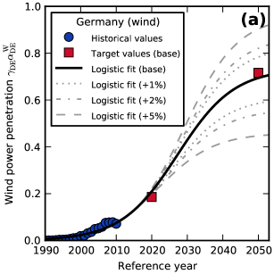
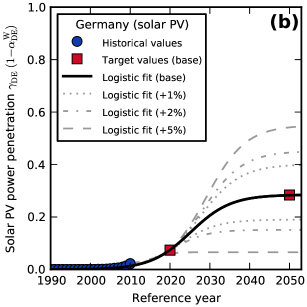
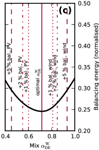
Figure 1: Logistic fits to historical and targeted wind (a) and solar PV (b) penetration in Germany 1990 - 2050. In panel (c), balancing energy as a function of the wind/solar mix for Germany is shown, for a renewable penetration of $\gamma_{\rm DE}=1.0$. The solid vertical line in this panel points out the balancing optimal mix, and the dotted, dashed-dotted and dashed lines indicate the mixes that lead to balancing needs increased by 1 %, 2 %, and 5 % of the load, respectively. These mixes are used for seven different 2050 targets in panels (a) and (b): the optimal mix corresponds to the base scenario (solid black lines), and the other mixes lead to the three wind heavy and three solar heavy logistic growth scenarios (grey broken lines). In calculating the balancing needs of single countries as in (c), imports and exports are not considered. Balancing is normalised by the average load.

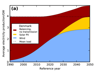
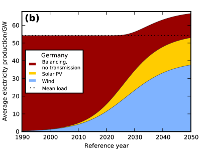
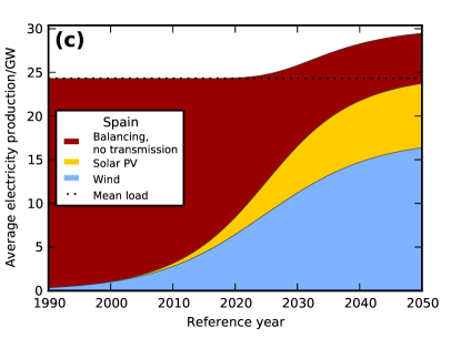
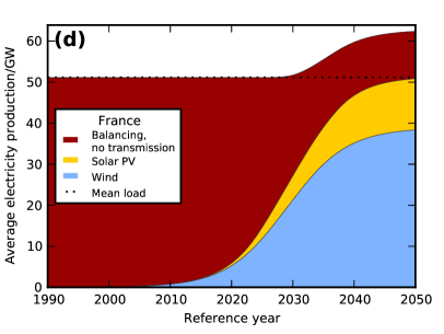
Figure 2: Logistic growth of wind (blue) and solar PV (yellow) power production, replacing conventional balancing, for (a) Denmark, (b) Germany, (c) Spain, and (d) France. Shown is the base scenario, where the single country balancing optimal mix is reached in 2050. The balancing energy (red) has been determined with the no-transmission layout. The conversion from the shares $\gamma_{n}\cdot\alpha^{\rm W}_{n}$ (wind) resp. $\gamma_{n}\cdot(1-\alpha^{\rm W}_{n})$ (solar PV) to average generation in $\rm GW$ is done using the 2007 load.

Alternative end-point mixes

To investigate whether the optimal mix changes as soon as transmission comes into play, we calculate logistic growth curves for a further range of end-point mixes $\alpha_{\rm W}$ of wind and solar energy. The final mix is varied over a range from roughly $\alpha^{\rm W}=0.40$ to $\alpha^{\rm W}=0.90$ wind share in six additional scenarios apart from the optimal mix base scenario: three solar heavy and three wind heavy scenarios, see Fig. 1c. In the base scenario, the end-point mix of each country is chosen as the mix that minimises the average balancing energy of the country on its own, i.e. without transmission. The wind heavy scenarios are defined by identifying the mixes to the right of the minimum that lead to increases in balancing by 1 %, 2 %, and 5 % of the average load. The three solar heavy scenarios are defined in analogy to the left of the minimum. All seven scenarios are indicated in Fig. 1c for Germany. Similar pictures emerge for the other countries; the different end-point mixes are given in Tab. LABEL:tab:endmix In the following, we examine the interplay between balancing and transmission in all seven scenarios with a focus on the base scenario, and then investigate the effect of transmission on the optimal mix comparing all scenarios.

2.3 Power transmission and balancing

The power transmission optimisation used in this paper applies a non-standard approach designed to maximise the utilisation of VRES while minimising the total need for transmission capacity. The optimisation is performed in two steps: The total balancing $B_{\rm tot}$ is minimised first. Secondly, the dissipation in the transmission network is minimised with $B_{\rm tot}$ constrained to its minimum value. Here, the two steps are described in short. Additional details can be found in [7].

The physical DC approximation to the full AC power flow, see e.g. [30], is used in order to calculate the balancing need at each node and the flow across each link. We conveniently assume equal susceptances for all the lines. In this case, the net export $P_{n}$ of each of the $N$ nodes can be expressed in terms of the $L$ flows $F_{l}$ via

$$P_{n}=\sum_{l=1}^{L}K_{nl}F_{l}.$$ (3)

Here, $K$ is the network’s incidence matrix, i.e.

$$K_{nl}=\begin{cases}\phantom{-}1&\text{ if link $l$ starts at node $n$}\\ -1&\text{ if link $l$ ends at node $n$}\\ \phantom{-}0&\text{ otherwise}\end{cases}$$ (4)

It is not difficult to generalise this to the case of non-uniform susceptances; these would appear in the entries of $K$. This formulation allows us to work in terms of the flows alone, since balancing can now be expressed as:

$$B_{\rm tot}=\sum_{n=1}^{N}(\Delta_{n}-(K\cdot F)_{n})_{-}=\sum_{n=1}^{N}B_{n}\,.$$ (5)

The balancing need $B_{n}$ at node $n$ is what is potentially left of a negative mismatch $\Delta_{n}$ after it has been reduced by the net imports $(K\cdot F)_{n}$.

If the line capacities are constrained by (possibly direction dependent) net transfer capacities (NTCs), $h_{-l}\leq F_{l}\leq h_{l}$, these constraints have to be included. We end up with two minimisation steps, the first representing maximal sharing of renewables, and the second minimizes transmission:

$$\begin{split}\text{Step 1: }&\min_{h_{-l}\leq F_{l}\leq h_{l}}\sum_{i=1}^{N}(\Delta_{n}-(K\cdot F)_{n})_{-}=B_{\rm min}\\ \text{Step 2: }&\min_{\begin{subarray}{c}h_{-l}\leq F_{l}\leq h_{l}\\ \sum_{i=1}^{N}(\Delta_{n}-(K\cdot F)_{n})_{-}=B_{\rm min}\end{subarray}}\sum_{l=1}^{L}F_{l}^{2}\end{split}$$ (6)

The network topology employed is shown in Fig. 3. We use five different transmission layouts, i.e. line capacity constraints: Zero transmission, transmission capacities as of today (shown in Fig. 3a), unconstrained transmission [7], and two layouts that are introduced and described in Sec. 3.3. See also Tab. LABEL:tab:linecap.

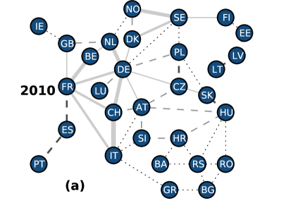
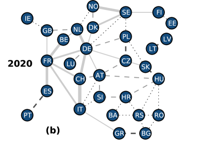
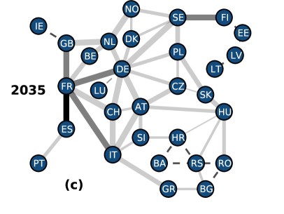
Figure 3: Network topology as used in our model: (a) present layout (winter 2010/2011) as reported by ENTSO-E plus the three new links GB-NL, NO-NL, and SE-PL [31, 32, 33, 34], (b)-(d) development of the 90 % benefit of transmission line capacities (see Sec. 3.3) for the years 2020, 2035, and 2050. Line style and thickness represents the larger one of the two net transfer capacities of each link. Line lengths and node sizes are not to scale.

3 Results

3.1 Time dependence of balancing energy for two fixed transmission layouts

We first focus on the base scenario, i.e. the single country balancing optimal mix. The impact of different end-point mixes will be discussed in Sec. 3.5. The first two transmission layouts we investigate are constant in time:

1. Zero transmission.

2. Today’s transmission layout: Net transfer capacities as of winter 2010/2011 from ENTSO-E, plus the three new links BritNed, NorNed, and SwePol [31, 32, 33, 34].

The resulting annual balancing energies for the single countries Denmark, Germany, Spain, and France are shown in Fig. 4a-d, in dark red for layout 1 and in red for layout 2. For each reference year, the annual balancing energy has been averaged over the available 8 years of weather and load data. Balancing needs rise quite steeply for the case of no power transmission, until it amounts to about 25 % of the average load in 2050. This is mitigated slightly if line capacities as of today are assumed. As discussed in more detail in Sec. 3.4, single countries show different intermediate behavior due to different trade opportunities. The corresponding figure for all of Europe is Fig. 5a, where balancing for layouts 1 and 2 is shown also in dark red and red, respectively.

For comparison, Fig. 5a also shows the theoretical minimum value for balancing as a thin, grey line. This would be obtained if the entire VRES production could be used to cover the load, i.e. if no excess production occurred. In this case, only a fraction of $(1-\gamma_{\text{avg.}}(t))=(1-\sum_{n}\gamma_{n}(t)\langle{L_{n}}\rangle/\langle{L_{EU}}\rangle)$ of the total load needs to be covered from balancing. It can be seen that the balancing needs of layout 1 depart already before 2030 from this optimal line, while layout 2 follows the optimum up to 2030.

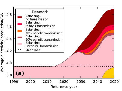
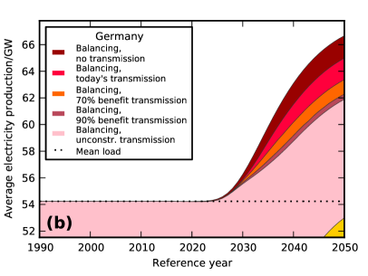
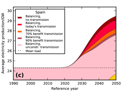
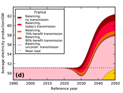
Figure 4: Zoom of Fig. 2, now also showing the reduction of annual balancing energy for various transmission layouts. For details on the transmission layouts, see Secs. 3.1–3.3.

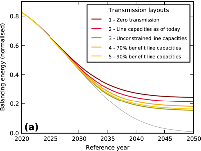
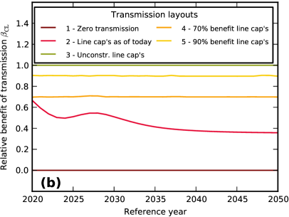
Figure 5: (a): Balancing energy vs. reference year for the various transmission layouts in the base scenario. Note how the balancing is reduced by 70 % (layout 4) or 90 % (layout 5) of what is achievable by suitable transmission grid extensions (see Sec. 3.3). This is also visible in panel (b), where the relative benefit of transmission is shown, cf. Eq. (7). In panel (a), the thin grey line shows the theoretical minimum balancing energy in each reference year, i.e. the average normalised load minus the average VRES penetration $\gamma$. Balancing energy is normalised by the mean load.

3.2 Maximum reduction of balancing energy for the time-dependent unconstrained transmission layout

The next transmission layout is chosen to be:

1. Unconstrained transmission.

It is possible to a posteriori associate a finite line capacity layout to unconstrained transmission, simply by setting the link capacities to the maximum value of the flow that is observed during the eight years of data, see Fig. 6a. Detailed numerical values can be found in Tab. LABEL:tab:linecap. Since in this layout a single hour’s flow determines the capacity of a link, it sometimes happens that these capacities drop from one reference year to the next for single links. This would correspond to a downgrade of an already built link, which is unrealistic. Such artifacts have therefore been removed, making the single links’ capacities monotonously increasing in reference year by keeping them at least at the levels reached in previous years.

To see the effect of this layout on balancing energy, we look again at Figs. 5a (green line) and 4a-d (pink area). We see that in Fig. 5a, balancing energy follows the theoretical minimum (grey line) about five years longer than layout 1, up to about 2032. Additionally, it is able to reduce the final balancing needs considerably, by about 40 % of its value at zero transmission. It cannot, however, reduce balancing energy down to zero: Power transmission is only able to match surpluses at some nodes with deficits at others. If there is a global deficit across all of Europe, balancing energy is needed no matter how strong the transmission grid. In Fig. 4d, it is seen that balancing for France drops temporarily such that combined own VRES generation and own balancing become lower than the average load. This is due to imports of VRES and will be discussed in more detail in Sec. 3.4.

Fig. 7a,b show in green the total necessary line upgrades to obtain layout 3. Fig. 7a depicts the total line capacities that need to be installed, and Fig. 7b shows the increments per five-year interval. For calculating the total transmission capacity, the larger one of the two NTC values of each link is used as a proxy to its physical capacity. These yield a sum of approximately $74\,\rm GW$ for the total line capacities installed today. The necessary total line capacities are plotted as multiples of this number. It is seen that line capacities for this layout would amount to almost twelve times of today’s installation in the end, and require a top installation speed of roughly adding today’s installation each year between 2025 and 2030.

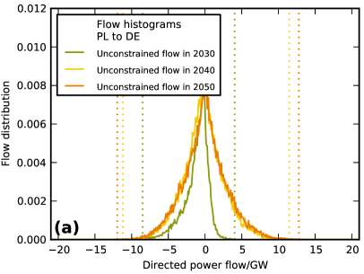
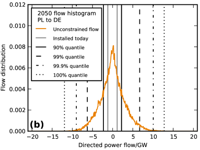
Figure 6: (a): Distributions of the unconstrained flow across the link between Germany and Poland for the years 2030, 2040 and 2050. Only non-zero flows are shown. The corresponding unconstrained line capacity layouts are assigned by setting the capacity of a given link to the maximum value that occurs in the unconstrained flow during the eight year data time series (dotted vertical lines). These values can be found in the last four columns of Tab. LABEL:tab:linecap. (b): 2050 unconstrained flow for the same link, with (direction specific) quantiles.

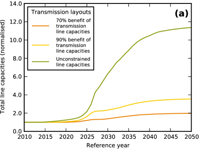
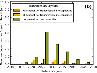
Figure 7: (a): Growth of total installed line capacity for the three time-dependent line capacity layouts unconstrained transmission (layout 3), 70 % benefit of transmission (layout 4), and 90 % benefit of transmission (layout 5). It is seen that layout 3 requires a final installation of almost twelve times of what we have today, layout 4 about twice as much, and layout 5 a little less than four times as much. (b): Five-year increment of line installations for the same three layouts. In both panels, the total installation is normalised by the installation of today (see Sec. 3.2 for details).

3.3 Two compromise transmission layouts

While the absence of new line investment of the two fixed layouts 1 and 2 makes them attractive, they lead to large balancing needs. Balancing needs are considerably reduced by the unimpeded power exchange of the unconstrained layout 3. This, however, requires huge investments in reinforced transmission lines. The idea is now to choose a line capacity layout which yields a certain reduction of balancing needs while keeping new line investments in a reasonable range.

The benefit of transmission for balancing reduction can be quantified in the following way: Denote a capacity layout by $C_{\text{L}}$, representing a set of net transfer line capacities. The total balancing $B_{\text{tot}}(C_{\text{L}})$ can then be understood as a function of $C_{\text{L}}$. The two extreme cases are the zero capacity layout $C_{\text{zero}}$ (layout 1), where all transmission capacities are set to zero, and the unconstrained layout $C_{\text{unconstrained}}$ (layout 3), where the transmission capacities are determined from what is necessary for unimpeded flow. The relative benefit of transmission $\beta(C_{\text{L}})$ of a generic layout $C_{\text{L}}$ can then be expressed as the reduction of balancing achieved by installing $C_{\text{L}}$ divided by the maximum possible benefit of transmission, which is obtained when switching from $C_{\text{zero}}$ to $C_{\text{unconstrained}}$:

$$\beta(C_{\text{L}})=\frac{B_{\text{tot}}(C_{\text{zero}})-B_{\text{tot}}(C_{\text{L}})}{B_{\text{tot}}(C_{\text{zero}})-B_{\text{tot}}(C_{\text{unconstrained}})}\;.$$ (7)

By construction, the relative benefit of transmission is zero for the zero capacity layout 1, and it is one for the unconstrained capacity layout 3. Fig. 5b illustrates the relative benefit of transmission for today’s capacity layout 2. It decreases with progressing reference years and converges from above to about $\beta(C_{\text{today}})=0.34$ for the final reference years.

Two new compromise transmission layouts are:

1. 70 % benefit of transmission capacities: For all links, fix a quantile of the unconstrained 2050 flows as transmission capacity (cf. Fig. 6 (b)), such that 70 % of the relative benefit of transmission is harvested (cf. Fig. 5 (a) and (b)).

2. 90 % benefit of transmission capacities: Analogously to 70 % benefit of transmission capacities.

There are a multitude of possible interpolations between zero transmission and unconstrained transmission that lead to the same desired balancing energy reduction and benefit of transmission as depicted in Fig. 5a+b. We choose the quantiles of the corresponding end-point (2050) unconstrained flow distribution because this policy has been found to perform best in terms of minimal transmission installations and maximum balancing reduction in [7]. For an illustration of the flow quantiles, see Fig. 6b for the link between Poland and Germany. We work with quantiles of the end-point flows rather than with quantiles of the unconstrained flow of the same year in order to consistently build up the capacity layout that is actually needed in the end. The quantile line capacities are capped by the unconstrained capacities of the corresponding years in order to avoid a premature installation of lines that are not used immediately. Furthermore, layouts 4 and 5 start from today’s NTCs, that is, no dismantling of existing lines is assumed.

The total transmission line capacities required to obtain the 70% and 90% benefit of transmission and the amount of new installations per five year intervals are shown in Fig. 7a and b. In addition, the capacity of each single link in the years 2020, 2030, 2040, and 2050 in the base scenario for the year-dependent line capacity layouts 3, 4, and 5 can be found in Tab. LABEL:tab:linecap. The build-up of the 90 % benefit of transmission layout is also illustrated in Fig. 3. About two and four times as much as what is installed today is needed to harvest 70 % and 90 % of the possible benefit of transmission, respectively. Both schemes seem within reach. For single links, the 90 % benefit layout agrees nicely with the results of [35], which finds e.g. a line capacity of $19.5\,\rm GW$ between Spain and France for the fully renewable stage, compared to $17.3\,\rm GW$ found in our base scenario. For the link between France and the UK, they report a final capacity $6\,\rm GW$, while we find $11.9\,\rm GW$. But this is due to the different grid topology they use, which includes an additional link from Great Britain to Norway with a capacity of $3.5\,\rm GW$, and a substantial offshore grid in the North Sea with a total capacity of $16.5\,\rm GW$.

Notably, the build-up in line capacities has to start no later than 2020 if the desired 70 % or 90 % benefit of transmission is to be harvested throughout the years. We have to keep in mind that the absolute reduction in balancing is small in the beginning (cf. Fig. 5), such that the total losses from not building the lines would be small at first. But, as balancing needs grow, the need for transmission capacity quickly increases. So it would be advisable to start the line build-up as soon as possible.

We take a combined look at Tab. LABEL:tab:logfit and Figs. 2, 5 and 7. Fig. 2 and Tab. LABEL:tab:logfit show that the main part of the wind installation growth takes place 2015-2035, while solar PV installations are a little later, about 2020-2040. Figs. 2 and 5a show an interesting feature: The onset of additional balancing energy beyond the minimum of $(1-\gamma_{\text{avg.}})$ times the average load can be postponed by transmission by five years. In order to achieve this, the main transmission line growth has to happen from 2025 to 2030, leading to the peak in new installations seen in Fig. 7b at that time.

3.4 Import and export opportunities

It is possible to investigate the effects of a strong transmission grid on the import and export opportunities of single countries. We only consider trade with VRES since other forms of electricity generation are not treated explicitly in our model. The transition at different times in different countries has some interesting effects. There are roughly three coordinates which determine export and import opportunities of a country, namely the size of its mean load, its position in the network (central or peripheral) and the time of transition to VRES with respect to its neighborhood.

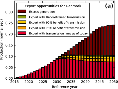
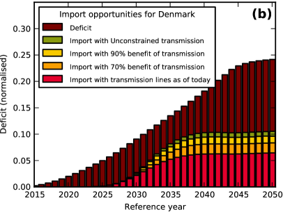
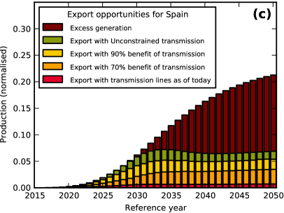
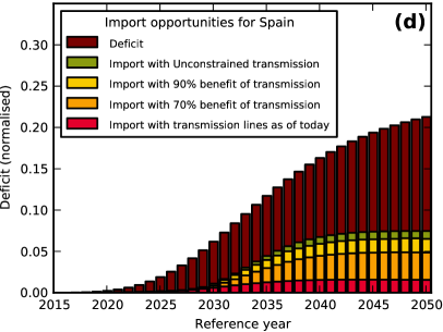
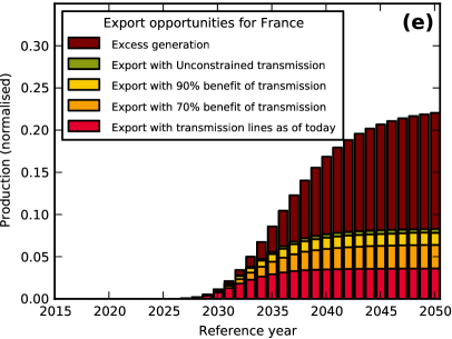
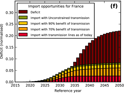
Figure 8: Export and import opportunities for selected countries, in the base scenario. Panels (a), (c), and (e) show the export opportunities in case of a domestic overproduction for Denmark, Spain, and France, respectively. Panels (b), (d), and (f) depict the import opportunities for the same countries, which are used to cover a domestic deficit or to replace domestic balancing.

Load size

A country’s load size influences the ratio of imported or exported energy to its deficit or surplus. A country with a high absolute load will experience high deficit as well as high excess. If its neighbours have a substantially smaller load, they will in most cases neither be able to absorb a large excess nor cover a large deficit. This means that the fraction of the deficit that can be covered by imports and the fraction of the excess that can be exported is smaller the larger a country’s load.

Position

The position of a country in the network is another factor that influences its trade opportunities. This point is a little more subtle and partly due to our power flow modelling which minimises the overall flow in the network. Neglect for a moment restricted transmission line capacities. Imagine a situation where some countries are in deficit and some are in excess, such that there is an overall shortage. The question is now which of the countries with a deficit gets the excess from those which see a surplus production. In a specific situation, the answer depends on the details of the distribution of excess and deficit in the network, but on average, transport of energy to a remote country causes more flow than to a central country, such that the central country will be preferred. The same goes for a situation where there is global excess, but some countries with a deficit: Central countries have a higher chance of exporting than peripheral ones, because this will on average cause less flow. Taking now limited transmission capacities into account, the situation is accentuated: A lot of flow to or from peripheral countries is not only suppressed by the flow minimisation, but may be altogether impossible.

Time of transition

Whether the transition to VRES occurs early or late in a country does not have an effect on the end-point import/export capabilities, but becomes important during the transition. If the transition in a country takes place early, it experiences deficit and excess situations earlier than its neighbours. For the first years, this means that in case of a deficit, neighbours are probably not able to export anything because they do not see excesses yet. On the other hand, because VRES generated electricity is shared wherever possible, if the early country has a surplus production, it can almost certainly export it to later neighbors, where it replaces local balancing. In short, an early transition may mean poor import opportunities, but on the other hand good export opportunities during the first years. These differences are subsequently diminished as all countries switch to VRES-based electricity supply, and then size and position become the dominant factors determining import and export opportunities.

In the reference year 2050, all countries reach a VRES share of (almost) $\gamma=1$. As shown in [7], even unlimited transmission can reduce the total balancing in Europe by only 40 % in the $\gamma=1$ case, due to the spatio-temporal correlations in the weather. This implies that in 2050, only 40 % of the total deficit can be covered by imports and equally only 40 % of the total excess can be exported. This statement is valid for the load-weighted average over all countries. Single countries see deviations due to their position and load size as explained above.

We take a look at three examples from the different classes which arise from these distinctions. We start with Denmark, which is small, central and an early adopter; see Figs. 8a and b as well as Fig. 4a. Denmark’s wind power installation covers on average more than 33 % of the load already today [36]. Up to now, the excess production can easily be exported into the neighbouring countries. On the import side, at first there are no neighbours willing to export any VRES generation because they can use everything domestically. This changes quickly as soon as the neighbours catch up with their VRES installation causing them excess production. Since the neighbours have a larger total production, resulting in more excess, the import opportunities are actually very good then, even leading to a dip in balancing energy between 2030 and 2040 for reinforced transmission grids, see Fig. 4a. Between 2045 and 2050, finally all countries reach a VRES share close to 100 %. This means that export opportunities are reduced: Since import can only replace balancing, but not domestic VRES production, it becomes less probable to find a customer for excess production.

For comparison, we now look at Spain (Figs. 8c and d and Fig. 4c), which also has ambitious VRES targets for the near future, but is peripheral. There is only one strong connection to Portugal. This connection does not improve the import/export capabilities of Spain much, since Portugal’s load is less than one fifth of the Spanish load, and it can therefore not absorb much of the Spanish fluctuations. We see that Spain starts similarly to Denmark with good potential export opportunities and no good chances to cover its deficits by import. However, there is a significant difference between the transmission capacities needed: While for Denmark today’s transmission capacities are already sufficient to export most of its excess, the weak link from Spain to France blocks almost all export if it is not reinforced. The same is true to a lesser degree for the import opportunities. In the further development, the import evolves appreciably different: Compared to Denmark, Spain’s import opportunities are poor. This is due to two reasons: Firstly, Spain has a bigger mean load. Its total deficit is therefore larger and harder to cover. Secondly, it is peripheral. In cases where there is only an insufficient supply of excess power which some countries want to export, while Spain and other countries have a deficit, the export flow will probably dry out before reaching Spain.

As a last example, we look at a central country which is large and relatively late, namely France (Figs. 8e and f and Fig. 4d). Its import opportunities are reasonably good for a country with a large load, but could be significantly improved by increased transmission capacities. The same holds for the export. As the transition to VRES is expected to be rather late in France, there are no deficits that cannot be covered by imports during the first years. In fact, VRES imports can already be used to replace balancing even before there is a significant domestic VRES installation, causing France to produce less than its own load from VRES and balancing. The rest can be covered by VRES imports (see the dip in Fig. 4d). On the other hand, France does not experience an export boom in the beginning.

3.5 Shift of optimal mix

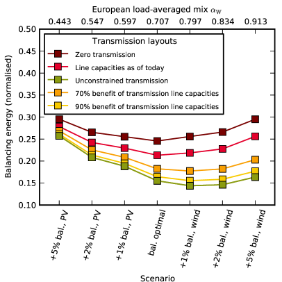
Figure 9: Annual European balancing energy for different average end-point mix scenarios for the year 2050. Note that the average mix can be read off the nonlinear top axis. Balancing is normalized by the average load.

So far we have used only the base scenario for the logistic growth of wind and solar power generation, where the 2050 end-point mix of each country is chosen such that it minimises the average balancing energy based on the zero transmission capacity layout. At the end of Sec. 2.2, six additional mix scenarios have been defined, with three of them having an increasingly larger share of wind power generation and the other three having an increasingly larger share of solar power generation. We will now use these six additional scenarios and investigate the impact of different relative mixes between wind and solar power generation on the combined balancing and transmission needs.

Fig. 9 shows the dependence of the annual European balancing energy on the different mix scenarios and on the different transmission layouts for the final reference year 2050. Once transmission is introduced, a higher wind share performs better in terms of balancing reduction. Compared to the base scenario, the two wind heavy $+1\,\%$ and $+2\,\%$ scenarios result in a lower European-wide balancing energy once the strong transmission layout types 3-5 are considered. The result is consistent with [7], where an optimal end-point mix $\alpha^{\rm W}_{\textup{agg.}}=0.822$ was found for an aggregated Europe with an unconstrained transmission capacity layout. The underlying reason for the shift towards more wind when large regions are interconnected is that the spatial correlation of wind power generation drops significantly over distances of 500 to 1000 km, while solar PV remains more correlated. The effect is well illustrated for the case of Sweden in [37]. When comparing the total balancing energy required in the base scenario and the $+1\,\%$ and $+2\,\%$ wind heavy scenarios, it becomes clear that the absolute difference between the three is relatively small for the strong transmission capacity layouts. This is again demonstrated in Fig. 10a, which shows the balancing energy as a function of the reference year, based on the 90 % benefit of transmission line capacities (layout 5).

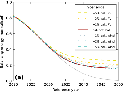
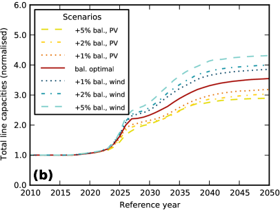
Figure 10: (a) Balancing energy and (b) total net transfer capacities vs. reference year for the base scenario, the three wind heavy and the three solar heavy scenarios, based on the 90 % benefit of transmission line capacities (layout 5). Total net transfer capacities have been normalized by the total installation of today. The dark red curves for the base scenario in panels (a) and (b) are identical to the yellow curves in Figs. 5a and 7a, respectively.

Fig. 10b illustrates the development of the total line capacities and reveals that a high wind share leads to higher transmission needs. This is due to the fact that for a high wind share, there is a high chance of covering a shortage in one country with excess from another. Solar PV power output, on the other hand, is much more correlated, being bound to the day-night pattern. Therefore, in case of a high share of solar PV, it is less probable that deficit and surplus production can cancel each other, implying less transmission needs.

The impact of the different scenarios for the relative mixes between wind and solar power generation on the combined balancing and transmission needs is summarised in Tab. 2. An opposing trend is observed: whereas the balancing energy decreases with an increasing, not-too-large share of wind power generation, it is the opposite for the total transmission capacity needs. This finding shows that when determining the complex features of a fully renewable energy system for Europe, it is not sufficient to look at isolated regions only, but also at the interplay between regions.

Table 2: Balancing energy needs and total transmission investment in 2050 resulting for different end-point mix scenarios, based on the 90 % benefit of transmission line capacities. All quantities are given as the relative deviation from the base scenario.

Scenario	Change in balancing energy	Change in transmission investment
$+5\,\%$ balancing, PV	$58.8\,$%	$-18.9\,$%
$+2\,\%$ balancing, PV	$30.0\,$%	$-14.8\,$%
$+1\,\%$ balancing, PV	$18.5\,$%	$-10.6\,$%
base	$0.0\,$%	$0.0\,$%
$+1\,\%$ balancing, wind	$-5.3\,$%	$9.1\,$%
$+2\,\%$ balancing, wind	$-3.5\,$%	$13.1\,$%
$+5\,\%$ balancing, wind	$7.9\,$%	$22.0\,$%

4 Conclusions

Using the logistic growth as an assumption for how the share of VRES in Europe grows from today up to a fully VRES-supplied European power system, we have investigated the required amount of transmission capacities that allow most of the excess from VRES to be shared across Europe during the transition. Most of the wind installation growth is expected to occur between 2015 and 2035, while the solar PV growth period is shifted by about five years. As soon as the total VRES share reaches levels of about 35 % in 2025, surplus production starts to rise without a strong transmission grid. This can be postponed by up to five years by transmission reinforcements, until the average VRES penetration has grown to more than 50 %. This line build-up has to start strongly during the early years from 2020 to 2030, and has to be continued on similar levels for fifteen more years in order for transmission to have a large overall system benefit. Such a transmission line investment is large, but appears to be feasible since the overall installation needs to reach only about two to four times of what we have today.

Reinforced transmission lines have several effects. Firstly, without any demand-side management and storage, transmission alone leads to a significant reduction in balancing energy needs by about one third. Secondly, the import and export opportunities become better for all countries, especially for those that are peripheral and go early for a high share of VRES, such as Ireland and Spain. Thirdly, the optimal mix of wind and solar changes: With more transmission, wind grid integration becomes easier, and so the optimum shifts from about a 70 % wind share to about 80 % wind share.

Import and export of electricity is greatly facilitated by a reinforced transmission grid. It has to be kept in mind, however, that while countries which increase their VRES penetration early benefit from the strong transmission lines during the first years, the export and import opportunities decrease once all countries have reached a high VRES share. This problem requires more attention in future research: most likely it can be diminished by the use of country-internal smart-energy systems, including storage, demand-side management, and conversion of excess electricity to heat.

This study is open for several possible future extensions. New transmission lines can be added to the topology of the employed network, which are either being built right now or planned in the near future, e.g. between Norway and Great Britain. New nodes can be added, reflecting Europe’s connections its neighbours. Dispatchable renewable sources, such as biomass and hydropower, could be included explicitly into the system. Note however, that the inclusion of hydro power in particular will lead to more transmission requirements, since the sites at which it is available are mainly Norway, Switzerland, and Austria. Taking these ideas further, a multi-dimensional optimization of the electricity supply can be investigated, including heterogeneous line capacities, balancing power capacities, balancing energy reserves, and renewable generation mix. Storage would be included as well, splitting it up into a local, small-capacity part, representing battery storage or demand-side management, and a large storage of seasonal capacity, representing e.g. hydrogen storage in salt caverns in Northern Germany, similar to the approach of [6]. This localized large storage facility will again lead to more power flow.

5 Acknowledgements

SB gratefully acknowledges financial support from O. and H. Stöcker, and GBA from DONG Energy and the Danish Advanced Technology Foundation. Furthermore, we would like to thank Uffe V. Poulsen and Tue V. Jensen for helpful discussions.

References

Appendix A Data tables

Table 3: End-point wind/solar mixes for three wind heavy, three solar heavy, and the single country optimal mix base scenario, expressed as the relative share $\alpha^{\rm W}$ of wind in VRES. The wind resp. solar heavy scenarios lead to balancing needs increased by 1 %, 2 % and 5 % of the average load when transmission is not included. The second last row shows the load-weighted average of the mixes over all single countries, and the last row shows the corresponding mixes for an aggregated Europe, where load and generation are shared without transmission limits.

		wind fraction $\alpha_{\rm W}$
country	avg. load/	solar heavy scenarios			base	wind heavy scenarios
	GW	$+5$ % bal.	$+2$ % bal.	$+1$ % bal.	opt. mix	$+1$ % bal.	$+2$ % bal.	$+5$ % bal.
AT	5.8	0.405	0.511	0.562	0.674	0.764	0.799	0.874
BA	3.1	0.413	0.523	0.574	0.683	0.765	0.797	0.872
BE	9.5	0.426	0.523	0.577	0.701	0.802	0.837	0.911
BG	5.1	0.368	0.484	0.540	0.659	0.753	0.789	0.869
CH	4.8	0.410	0.522	0.575	0.691	0.785	0.819	0.891
CZ	6.6	0.439	0.548	0.600	0.713	0.802	0.836	0.911
DE	54.2	0.454	0.551	0.601	0.716	0.810	0.849	0.934
DK	3.9	0.474	0.569	0.617	0.732	0.829	0.867	0.951
EE	1.5	0.570	0.671	0.717	0.813	0.895	0.931	1.000
ES	24.3	0.461	0.556	0.600	0.697	0.794	0.837	0.933
FI	9.0	0.531	0.638	0.689	0.796	0.878	0.912	0.991
FR	51.1	0.511	0.610	0.657	0.755	0.845	0.886	0.979
GB	38.5	0.547	0.641	0.687	0.787	0.873	0.911	0.996
GR	5.8	0.369	0.479	0.530	0.642	0.739	0.781	0.871
HR	1.6	0.351	0.464	0.520	0.640	0.734	0.768	0.840
HU	4.4	0.390	0.496	0.548	0.663	0.753	0.786	0.860
IE	3.2	0.514	0.606	0.651	0.754	0.843	0.880	0.962
IT	34.5	0.390	0.492	0.540	0.647	0.744	0.786	0.877
LT	1.5	0.538	0.640	0.688	0.789	0.874	0.912	0.997
LU	0.7	0.421	0.533	0.588	0.707	0.801	0.835	0.906
LV	0.7	0.575	0.672	0.717	0.811	0.894	0.932	1.000
NL	11.5	0.451	0.546	0.596	0.716	0.813	0.851	0.933
NO	13.7	0.614	0.710	0.755	0.849	0.926	0.961	1.000
PL	15.2	0.472	0.577	0.629	0.740	0.830	0.868	0.952
PT	4.8	0.412	0.511	0.559	0.661	0.756	0.797	0.887
RO	5.4	0.423	0.532	0.583	0.689	0.777	0.816	0.904
RS	3.9	0.422	0.530	0.582	0.695	0.783	0.815	0.887
SE	16.6	0.572	0.672	0.719	0.818	0.901	0.937	1.000
SI	1.4	0.372	0.482	0.535	0.651	0.743	0.778	0.851
SK	3.1	0.438	0.546	0.597	0.707	0.792	0.825	0.901
Eur. (agg.)	345.3	0.611	0.698	0.738	0.822	0.907	0.945	1.000
Eur. (avg.)	345.3	0.475	0.575	0.623	0.730	0.821	0.859	0.942

Table 4: Logistic growth of VRES installation, for the base scenario. Shown are the penetrations of wind and solar PV production in the total electricity production, for the reference years 2015-2050 in five-year steps, and the fit parameters, see Eq. (2). The last two rows contain the average development in Europe.

country	penetration in electricity production								fit parameters
	2015	2020	2025	2030	2035	2040	2045	2050	$a$	$b$	$m$	$y_{0}$
AT (wind)	0.04	0.09	0.17	0.30	0.44	0.55	0.62	0.66	2.1e-05	0.69	0.16	1967
AT (PV)	0.00	0.00	0.04	0.12	0.21	0.29	0.32	0.33	1.1e-11	0.33	0.50	1980
BA (wind)	0.00	0.04	0.20	0.38	0.55	0.67	0.68	0.68	2.5e-09	0.68	0.56	1990
BA (PV)	0.00	0.02	0.08	0.15	0.23	0.30	0.31	0.32	4.7e-09	0.32	0.34	1975
BE (wind)	0.03	0.10	0.23	0.40	0.56	0.65	0.69	0.70	5.7e-07	0.70	0.22	1965
BE (PV)	0.00	0.01	0.04	0.12	0.19	0.26	0.29	0.30	3.8e-08	0.30	0.30	1978
BG (wind)	0.03	0.07	0.18	0.34	0.50	0.60	0.64	0.66	1.1e-05	0.66	0.22	1979
BG (PV)	0.00	0.01	0.08	0.16	0.25	0.32	0.34	0.34	1.1e-10	0.34	0.47	1980
CH (wind)	0.00	0.01	0.12	0.30	0.47	0.64	0.69	0.69	4.2e-13	0.69	0.61	1980
CH (PV)	0.00	0.01	0.06	0.13	0.21	0.28	0.31	0.31	6.3e-10	0.31	0.41	1979
CZ (wind)	0.00	0.02	0.10	0.27	0.45	0.63	0.70	0.71	1.3e-08	0.71	0.35	1979
CZ (PV)	0.01	0.02	0.06	0.13	0.20	0.26	0.28	0.29	1.7e-06	0.29	0.24	1979
DE (wind)	0.13	0.21	0.31	0.43	0.53	0.61	0.66	0.69	7.5e-05	0.73	0.13	1954
DE (PV)	0.03	0.07	0.14	0.21	0.25	0.27	0.28	0.28	3.5e-05	0.28	0.20	1979
DK (wind)	0.38	0.49	0.58	0.64	0.68	0.71	0.72	0.73	1.8e-02	0.74	0.12	1984
DK (PV)	0.00	0.00	0.01	0.06	0.13	0.20	0.26	0.27	4.0e-14	0.27	0.58	1980
EE (wind)	0.02	0.05	0.13	0.28	0.47	0.63	0.71	0.75	5.0e-06	0.77	0.21	1974
EE (PV)	0.00	0.00	0.01	0.06	0.12	0.18	0.23	0.24	4.7e-13	0.24	0.53	1980
ES (wind)	0.18	0.27	0.36	0.46	0.54	0.61	0.65	0.67	1.0e-03	0.71	0.11	1966
ES (PV)	0.04	0.08	0.15	0.22	0.27	0.29	0.30	0.30	2.0e-04	0.30	0.20	1988
FI (wind)	0.01	0.06	0.20	0.40	0.60	0.74	0.78	0.79	5.5e-06	0.80	0.29	1987
FI (PV)	0.00	0.00	0.01	0.05	0.10	0.15	0.20	0.20	2.2e-13	0.20	0.54	1980
FR (wind)	0.04	0.10	0.23	0.42	0.59	0.69	0.73	0.75	6.0e-05	0.76	0.21	1983
FR (PV)	0.00	0.01	0.05	0.11	0.18	0.23	0.24	0.24	1.9e-08	0.25	0.34	1980
GB (wind)	0.08	0.21	0.40	0.59	0.71	0.76	0.78	0.79	7.9e-05	0.79	0.22	1982
GB (PV)	0.00	0.01	0.05	0.10	0.15	0.20	0.21	0.21	8.6e-12	0.21	0.51	1980
GR (wind)	0.13	0.25	0.39	0.51	0.59	0.62	0.63	0.64	4.1e-05	0.64	0.19	1970
GR (PV)	0.01	0.05	0.14	0.23	0.32	0.35	0.36	0.36	4.9e-08	0.36	0.36	1980
HR (wind)	0.01	0.04	0.14	0.29	0.45	0.58	0.62	0.64	1.0e-05	0.64	0.27	1988
HR (PV)	0.00	0.02	0.10	0.19	0.28	0.35	0.36	0.36	1.3e-12	0.36	0.61	1981
HU (wind)	0.01	0.03	0.11	0.26	0.43	0.57	0.64	0.66	4.6e-07	0.67	0.26	1977
HU (PV)	0.00	0.00	0.05	0.14	0.22	0.30	0.34	0.34	9.1e-18	0.34	0.82	1980
IE (wind)	0.14	0.24	0.35	0.48	0.58	0.66	0.71	0.74	1.6e-04	0.77	0.13	1960
IE (PV)	0.00	0.00	0.01	0.06	0.12	0.18	0.24	0.25	1.5e-14	0.25	0.60	1980
IT (wind)	0.03	0.07	0.15	0.28	0.43	0.55	0.61	0.64	1.6e-05	0.66	0.19	1975
IT (PV)	0.01	0.03	0.09	0.18	0.27	0.33	0.35	0.35	2.2e-06	0.35	0.26	1983
LT (wind)	0.04	0.09	0.21	0.39	0.57	0.68	0.73	0.75	6.8e-06	0.76	0.20	1972
LT (PV)	0.00	0.00	0.04	0.10	0.16	0.22	0.24	0.24	4.9e-18	0.24	0.83	1980
LU (wind)	0.01	0.04	0.12	0.28	0.46	0.61	0.68	0.70	1.5e-06	0.71	0.24	1977
LU (PV)	0.00	0.01	0.05	0.11	0.19	0.25	0.28	0.29	3.1e-07	0.29	0.26	1978
LV (wind)	0.04	0.11	0.25	0.44	0.62	0.71	0.74	0.75	6.9e-05	0.76	0.23	1987
LV (PV)	0.00	0.00	0.03	0.09	0.15	0.21	0.24	0.24	8.4e-19	0.24	0.85	1980
NL (wind)	0.11	0.24	0.40	0.55	0.64	0.69	0.71	0.71	8.3e-04	0.72	0.19	1988
NL (PV)	0.00	0.00	0.01	0.07	0.14	0.21	0.27	0.28	2.0e-13	0.28	0.55	1980
NO (wind)	0.05	0.19	0.40	0.61	0.78	0.83	0.85	0.85	2.1e-05	0.85	0.30	1988
NO (PV)	0.00	0.00	0.00	0.04	0.07	0.11	0.14	0.15	1.2e-13	0.15	0.54	1980
PL (wind)	0.03	0.09	0.23	0.42	0.59	0.69	0.72	0.74	6.2e-05	0.74	0.24	1988
PL (PV)	0.00	0.00	0.01	0.06	0.13	0.19	0.25	0.26	1.2e-11	0.26	0.46	1980
PT (wind)	0.17	0.27	0.38	0.48	0.56	0.61	0.64	0.65	1.4e-04	0.67	0.13	1959
PT (PV)	0.01	0.04	0.11	0.20	0.28	0.32	0.34	0.34	7.3e-07	0.34	0.28	1980
RO (wind)	0.02	0.11	0.29	0.46	0.62	0.68	0.69	0.69	9.5e-06	0.69	0.36	1993
RO (PV)	0.00	0.00	0.06	0.14	0.22	0.29	0.31	0.31	3.9e-15	0.31	0.70	1980
RS (wind)	0.00	0.04	0.21	0.38	0.56	0.68	0.69	0.69	1.7e-08	0.70	0.57	1994
RS (PV)	0.00	0.02	0.09	0.17	0.24	0.30	0.30	0.30	2.9e-11	0.31	0.52	1981
SE (wind)	0.04	0.09	0.20	0.38	0.58	0.71	0.78	0.81	2.3e-05	0.83	0.20	1977
SE (PV)	0.00	0.00	0.01	0.04	0.09	0.13	0.17	0.18	1.3e-13	0.18	0.55	1980
SI (wind)	0.00	0.01	0.14	0.30	0.47	0.62	0.65	0.65	5.4e-14	0.65	0.67	1980
SI (PV)	0.00	0.01	0.06	0.15	0.24	0.32	0.35	0.35	1.7e-10	0.35	0.45	1980
SK (wind)	0.00	0.02	0.13	0.31	0.49	0.66	0.70	0.71	1.6e-10	0.71	0.47	1980
SK (PV)	0.00	0.01	0.07	0.15	0.22	0.28	0.29	0.29	1.5e-13	0.29	0.63	1980
Avg. (wind)	0.07	0.15	0.27	0.43	0.57	0.66	0.70	0.72	-	-	-	-
Avg. (PV)	0.01	0.03	0.07	0.13	0.20	0.24	0.27	0.27	-	-	-	-

Table 5: Line capacities for the reference year-dependent transmission capacity layouts 3, 4, and 5 (see Secs. 3.1–3.3) according to the base scenario in the years 2020, 2030, 2040, and 2050. Net transfer capacities are given in MW.

link	today	70 % benefit				90 % benefit				unconstrained
		2020	2030	2040	2050	2020	2030	2040	2050	2020	2030	2040	2050
	470	470	1210	1890	2030	470	2440	3460	3680	470	4900	12270	13720
AT $\rightleftarrows$ CH	1200	1200	1350	1990	2100	1200	2430	3310	3510	1200	6250	10020	11050
	600	600	1580	2630	2850	600	3480	5000	5350	600	8660	15500	16100
AT $\rightleftarrows$ CZ	1000	1000	1500	2530	2740	1000	3280	4570	4850	1000	5650	10480	11720
	2000	2000	2370	3940	4280	2000	5300	7830	8450	2000	11150	25300	28170
AT $\rightleftarrows$ DE	2200	2200	2630	4180	4460	2200	5320	7260	7670	2200	10520	17420	17420
	800	800	1450	2240	2410	800	2850	3900	4130	800	6930	8910	9590
AT $\rightleftarrows$ HU	800	800	1310	2220	2380	800	2980	4690	5120	800	7340	19300	19860
	220	220	2200	3390	3600	220	4250	5710	6050	220	7830	13840	15460
AT $\rightleftarrows$ IT	285	290	2190	3560	3820	290	4590	6560	6990	290	10850	19050	21450
	900	900	1240	2000	2160	900	2570	3410	3600	900	4360	7400	7830
AT $\rightleftarrows$ SI	900	900	1180	1950	2140	900	2600	3910	4220	900	7000	14000	15500
	600	600	600	950	1040	600	1300	2020	2210	600	3920	7100	7290
BA $\rightleftarrows$ HR	600	600	620	930	990	600	1180	1590	1670	600	2580	3780	3850
	350	350	420	730	790	350	980	1460	1580	350	2070	4170	4230
BA $\rightleftarrows$ RS	450	450	450	640	680	450	810	1140	1210	450	2620	3850	4020
	550	550	1040	1720	1840	550	2270	3410	3660	550	6080	15540	15780
BG $\rightleftarrows$ GR	500	570	1180	1800	1900	1270	2240	3060	3270	2320	7290	10280	10560
	600	600	600	940	1030	600	1300	1960	2110	600	4800	7220	7220
BG $\rightleftarrows$ RO	600	600	710	1060	1130	600	1300	1740	1830	600	3050	4820	5260
	450	450	790	1410	1540	450	1960	3010	3250	450	6330	10800	11230
BG $\rightleftarrows$ RS	300	300	1080	1540	1620	300	1840	2340	2450	300	3420	5350	5790
	3500	3500	3500	3810	4070	3500	4910	7100	7620	3500	9990	20700	22060
CH $\rightleftarrows$ DE	1500	1500	2450	3860	4120	1500	4890	6760	7210	1500	9450	14730	16360
	4165	4170	4170	4170	4170	4170	4890	6530	6860	4170	8660	13850	14950
CH $\rightleftarrows$ IT	1810	1810	2310	3790	4100	1810	5000	7360	7890	1810	10380	23390	26300
	2300	2300	2300	2300	2340	2300	2840	4210	4580	2300	5620	14760	16820
CZ $\rightleftarrows$ DE	800	800	1580	2460	2620	800	3070	4180	4470	800	8370	10870	11810
	2200	2200	2200	2200	2200	2200	2200	2200	2340	2200	3530	5030	5360
CZ $\rightleftarrows$ SK	1200	1200	1200	1310	1420	1200	1710	2530	2740	1200	3710	8200	8790
	1550	1550	1550	2250	2400	1550	2900	4050	4310	1550	9210	11590	12130
DE $\rightleftarrows$ DK	2085	2090	2090	2430	2610	2090	3180	4500	4830	2090	5350	10470	12920
	980	980	980	980	980	980	980	980	980	980	980	980	980
DE $\rightleftarrows$ LU	NRL	980	980	980	980	980	980	980	980	980	980	1360	1500
	600	600	2310	3630	3860	600	4620	6370	6760	600	13830	16430	16580
DE $\rightleftarrows$ SE	610	610	2240	3710	4030	610	4930	7090	7580	610	5020	16420	20370
	750	750	750	750	750	750	750	980	1040	750	1730	2500	2580
EE $\rightleftarrows$ LV	850	850	850	850	850	850	850	1060	1120	850	1120	2650	2910
	350	350	490	800	860	350	1060	1560	1680	350	3000	4230	4350
FI $\rightleftarrows$ EE	350	350	510	810	870	350	990	1520	1660	350	990	4230	5350
	1650	1650	2650	4800	5240	1650	6570	9650	10390	1650	8280	22690	25290
FI $\rightleftarrows$ SE	2050	2050	3100	4790	5100	2050	5990	7770	8170	2050	12130	15070	15420
	3400	3400	3400	3400	3400	3400	3730	5310	5720	3400	11000	17130	18820
FR $\rightleftarrows$ BE	2300	2300	2300	3010	3200	2300	3810	5360	5770	2300	6650	13060	13900
	3200	3200	3200	3790	4090	3200	4800	6720	7120	3200	13990	21760	25250
FR $\rightleftarrows$ CH	1100	1100	2330	3550	3810	1100	4470	6140	6550	1100	10280	22430	25370
	2700	2700	3670	5810	6230	2700	7480	10590	11280	2700	20680	33290	35450
FR $\rightleftarrows$ DE	3200	3200	3380	5400	5810	3200	7000	9850	10560	3200	14430	29190	29650
	1300	1300	5210	8000	8530	1300	10120	14040	14950	1300	17440	37250	37860
FR $\rightleftarrows$ ES	500	730	3490	6550	7280	3780	9310	15420	16880	15070	49600	65360	72750
	2000	2000	3320	5450	5820	2000	6950	9650	10270	2000	20400	30070	31470
FR $\rightleftarrows$ GB	2000	2000	4150	6520	6970	2000	8350	11280	11940	2000	16610	25930	27960
	2575	2580	4180	6440	6860	2580	8070	10900	11530	2580	20930	31670	35380
FR $\rightleftarrows$ IT	995	1000	3750	5990	6380	1000	7820	11570	12450	1000	16010	36580	39900
	450	450	620	1040	1130	450	1340	1830	1930	450	3230	4510	4510
GB $\rightleftarrows$ IE	80	80	700	1070	1120	80	1240	1680	1750	80	1240	3290	4230
	500	630	1680	2900	3110	1810	3910	5930	6440	2320	14070	21510	21670
GR $\rightleftarrows$ IT	500	500	2140	3100	3290	500	3780	4790	5010	500	8200	9880	11900
	800	800	800	1160	1240	800	1520	2200	2370	800	4150	7200	7310
HR $\rightleftarrows$ HU	1200	1200	1200	1200	1200	1200	1420	1910	2010	1200	2240	4260	4770
	350	350	680	990	1050	350	1210	1560	1630	350	2480	3200	3230
HR $\rightleftarrows$ RS	450	450	530	900	980	450	1210	1900	2040	450	3910	7780	7920
	1000	1000	1000	1520	1620	1000	2010	3140	3370	1000	5260	12290	13030
HR $\rightleftarrows$ SI	1000	1000	1000	1570	1690	1000	2030	2680	2830	1000	5170	6670	7100
	600	600	1000	1600	1710	600	2090	2870	3050	600	3740	6330	6580
HU $\rightleftarrows$ RS	700	700	930	1590	1700	700	2120	3320	3640	700	7110	12760	13280
	600	600	1750	3100	3350	600	4150	6290	6840	600	12030	23040	24970
HU $\rightleftarrows$ SK	1300	1300	1810	3080	3310	1300	4030	5550	5920	1300	6870	12890	14150
	160	160	1250	1930	2060	160	2450	3400	3620	160	5550	11410	12280
IT $\rightleftarrows$ SI	580	580	1220	1810	1910	580	2240	3110	3340	580	5030	12570	12890
	1300	1300	1300	1300	1300	1300	1300	1300	1300	1300	1300	1680	1720
LV $\rightleftarrows$ LT	1500	1500	1500	1500	1500	1500	1500	1500	1500	1500	1500	1840	2190
	2400	2400	2400	2570	2720	2400	3280	4620	4920	2400	7210	12100	13080
NL $\rightleftarrows$ BE	2400	2400	2400	2560	2750	2400	3390	4860	5210	2400	9970	14340	15980
	3000	3000	3000	3270	3540	3000	4260	5860	6240	3000	10310	17240	19010
NL $\rightleftarrows$ DE	3850	3850	3850	3850	3850	3850	3850	5170	5550	3850	10590	16370	19280
	1000	1000	2340	4020	4350	1000	5270	7450	7930	1000	11700	24870	27920
NL $\rightleftarrows$ GB	1000	1000	3120	5060	5400	1000	6450	8780	9270	1000	15420	24320	25300
	700	700	2670	3950	4180	700	4870	6770	7190	700	14710	18290	19640
NL $\rightleftarrows$ NO	700	700	2470	3930	4170	700	4940	6800	7210	700	9720	17990	20250
	950	950	1350	2000	2110	950	2420	3090	3230	950	4310	7530	8120
NO $\rightleftarrows$ DK	950	950	1190	1680	1770	950	2030	2600	2730	950	5630	6850	7510
	3595	3600	3600	3600	3600	3600	3600	3810	4020	3600	9100	12180	12240
NO $\rightleftarrows$ SE	3895	3900	3900	3900	3900	3900	3900	3900	3900	3900	5500	11950	13160
	1800	1800	1800	1990	2110	1800	2510	3450	3680	1800	3490	8010	8880
PL $\rightleftarrows$ CZ	800	800	1170	1880	2020	800	2410	3370	3580	800	5810	10610	11570
	1100	1100	1510	2450	2630	1100	3170	4340	4630	1100	4040	11470	12780
PL $\rightleftarrows$ DE	1200	1200	1630	2540	2730	1200	3250	4380	4640	1200	8500	11260	11960
	1	0	1900	3000	3180	0	3760	5220	5580	0	8630	17090	18120
PL $\rightleftarrows$ SE	600	600	1920	3140	3410	600	4080	5900	6270	600	7680	15850	16860
	600	600	1730	2630	2790	600	3280	4520	4790	600	5550	10930	11430
PL $\rightleftarrows$ SK	500	500	1530	2520	2730	500	3380	4940	5350	500	7990	16890	17940
	1500	1500	1500	2040	2190	1500	2650	3840	4110	2250	7720	11780	12150
PT $\rightleftarrows$ ES	1700	1700	1700	1900	2040	1700	2430	3240	3400	2540	5370	7850	7850
	700	700	1240	2160	2350	700	2910	4470	4870	700	9250	15870	16330
RO $\rightleftarrows$ HU	700	700	1400	2100	2240	700	2630	3490	3670	700	4640	7160	7570
	700	700	700	910	1000	700	1250	1940	2120	700	3650	5480	5680
RO $\rightleftarrows$ RS	500	500	660	900	950	500	1080	1390	1470	500	2750	3830	3830
	1980	1980	1980	1980	1980	1980	2170	3060	3240	1980	2210	7040	8230
SE $\rightleftarrows$ DK	2440	2440	2440	2440	2440	2440	2440	2900	3070	2440	6590	7340	7340

References

- [1] McKinsey & Company, KEMA, The Energy Futures Lab at Imperial College London, Oxford Economics, and ECF. Roadmap 2050 – A practical guide to a prosperous, low-carbon Europe. Technical report, European Climate Foundation, http://www.roadmap2050.eu/downloads, April 2010. Online, retrieved June 2012.
- [2] M. Z. Jacobson and M. A. Delucchi. A Path to Sustainable Energy by 2030. Scientific American, 301:58–65, 2009.
- [3] D. Heide, L. von Bremen, M. Greiner, C. Hoffmann, M. Speckmann, and S. Bofinger. Seasonal optimal mix of wind and solar power in a future, highly renewable Europe. Renewable Energy, 35:2483–2489, November 2010.
- [4] D. Heide, M. Greiner, L. von Bremen, and C. Hoffmann. Reduced storage and balancing needs in a fully renewable European power system with excess wind and solar power generation. Renewable Energy, 36:2515–2523, September 2011.
- [5] K. Schaber, F. Steinke, T. Hamacher, and P. Mühlich. Parametric study of variable renewable energy integration in Europe: Advantages and costs of transmission grid extensions. Energy Policy, 42:498–508, December 2011.
- [6] M. G. Rasmussen, G. B. Andresen, and M. Greiner. Storage and balancing synergies in a fully or highly renewable pan-European power system. Energy Policy, 51:642–651, December 2012.
- [7] R. A. Rodriguez, S. Becker, G. B. Andresen, D. Heide, and M. Greiner. Transmission needs across a fully renewable European power system. Submitted for review, 2013. Preprint available on http://arxiv.org/abs/1306.1079.
- [8] K. Schaber, F. Steinke, and T. Hamacher. Transmission grid extensions for the integration of variable renewable energies in Europe: Who benefits where? Energy Policy, 43:123–135, February 2012.
- [9] M. Fürsch, S. Hagspiel, C. Jägemann, S. Nagl, D. Lindenberger, L. Glotzbach, E. Tröster, and T. Ackermann. Roadmap 2050 - a closer look. Technical report, energynautics and Institute for Energy Economy at the University of Cologne, http://www.energynautics.com/news/, October 2011.
- [10] F. Steinke, P. Wolfrum, and C. Hoffmann. Grid vs. storage in a 100% renewable Europe. Renewable Energy, 50:826 – 832, February 2013.
- [11] ENTSO-E. Country-specific hourly load data. https://www.entsoe.eu/resources/data-portal/consumption/, 2011.
- [12] S. Bofinger, L. von Bremen, K. Knorr, K. Lesch, K. Rohrig, Y.-M. Saint-Drenan, and M. Speckmann. Raum-zeitliche Erzeugungsmuster von Wind- und Solarenergie in der UCTE-Region und deren Einfluss auf elektrische Transportnetze: Abschlussbericht für Siemens Zentraler Forschungsbereich (Temporal and Spatial Generation Patterns of Wind and Solar Energy in the UCTE-Region. Impacts of these on the Electricity Transmission Grid). Technical report, Institut für Solare Energieversorgungstechnik, ISET e.V., Kassel, November 2008.
- [13] Eurostat. http://epp.eurostat.ec.europa.eu, 2012. Online, retrieved January 2012.
- [14] International Energy Agency. Energy in the Western Balkans, 2008.
- [15] EU member countries. National Renewable Energy Action Plans. http://ec.europa.eu/energy/renewables/action_plan_en.htm, 2010. Online, retrieved January 2012.
- [16] Energiaftalen 22. marts 2012. http://www.ens.dk, 2012. Online, retrieved November 2012.
- [17] Schweizerische Eidgenossenschaft - Der Bundesrat. Energieperspektiven 2050, May 2011.
- [18] A. Kirchner, F Ess, and A. Piégsa. Energieszenarien für die Schweiz bis 2050. Technical report, prognos AG Basel, May 2011.
- [19] Croatian Parliament. Energy Strategy of Croatia. Official Gazette of the Croatian Parliament, October 2009.
- [20] SINTEF (Norwegian foundation for scientific and industrial research). http://www.sintef.no/wind, 2012. Online, retrieved September 2012.
- [21] European Commission. A roadmap for moving to a competitive low carbon economy in 2050. Technical report, EC, March 2011.
- [22] B. Lehner, G. Czisch, and S. Vassolo. The impact of global change on the hydropower potential of Europe: a model-based analysis. Energy Policy, 33(7):839 – 855, 2005.
- [23] L. W. M. Beurskens, M. Hekkenberg, and P. Vethman. Renewable Energy Projections as Published in the National Renewable Energy Action Plans of the European Member States. Technical report, Energy research Centre of the Netherlands, http://ecn.nl/nreap, November 2011. Online, retrieved September 2012.
- [24] ITER Organization. http://www.iter.org/proj/iterandbeyond, 2012. Online, retrieved May 2012.
- [25] A. Grübler. The Rise and Fall of Infrastructures. Physica-Verlag, Heidelberg, 1990.
- [26] S. Moore and J. L. Simon. The Greatest Century that ever was. Policy Analysis, 1999.
- [27] A. Grübler, N. Nakićenović, and D. G. Victor. Dynamics of energy technologies and global change. Energy Policy, 5:247–280, May 1999.
- [28] C. Wilson and A. Grübler. Lessons from the history of technological change for clean energy scenarios and policies. Natural Resources Forum, 35:165–184, August 2011.
- [29] Technology Data for Energy Plants. Technical report, The Danish Energy Agency (Energistyrelsen) and Energinet.dk, http://www.ens.dk, May 2012. Online, retrieved October 2012.
- [30] B. Oswald and D. Oeding. Elektrische Kraftwerke und Netze. Springer-Verlag, Berlin Heidelberg New York, 6 edition, 2004.
- [31] ENTSO-E. Indicative values for Net Transfer Capacities (NTC) in Continental Europe. European Transmission System Operators. https://www.entsoe.eu/resources/ntc-values/ntc-matrix, February 2011. Online, retrieved February 2012.
- [32] BritNed Construction. http://www.britned.com/BritNed/AboutUs/Construction, 2013. Online, retrieved July 2013.
- [33] NorNed – første markedsdag mandag. http://www.statnett.no/no/Nyheter-og-media/Nyhetsarkiv/Nyhetsarkiv---20%08/NorNed--forste-markedsdag-mandag-/, 2008. Online, retrieved July 2013.
- [34] SwePol Link HVDC interconnection project. http://www.abb.com/industries/ap/db0003db004333/c84945b54aa6cfb8c125774%a00486402.aspx, 2013. Online, retrieved July 2013.
- [35] E. Tröster, R. Kuwahata, and T. Ackermann. European grid study 2030/2050. Technical report, energynautics GmbH, http://www.energynautics.com/news/, January 2011. Online, retrieved November 2012.
- [36] Månedlig elforsyningsstatistik, summary tab B58-B72. http://www.ens.dk, 2012. Online, retrieved November 2012.
- [37] J. Widén. Correlations between large-scale solar and wind power in a future scenario for sweden. IEEE Transactions on Sustainable Energy, 2(2):177–184, 2011.