Linear bound in terms of maxmaxflow
for the chromatic roots of series-parallel graphs

Abstract

We prove that the (real or complex) chromatic roots of a series-parallel graph with maxmaxflow $\Lambda$ lie in the disc $|q-1|<(\Lambda-1)/\log 2$. More generally, the same bound holds for the (real or complex) roots of the multivariate Tutte polynomial when the edge weights lie in the “real antiferromagnetic regime” $-1\leq v_{e}\leq 0$. This result is within a factor $1/\log 2\approx 1.442695$ of being sharp.

Key Words: Chromatic polynomial; multivariate Tutte polynomial; antiferromagnetic Potts model; chromatic roots; maxmaxflow; series-parallel graph.

Mathematics Subject Classification (MSC 2010) codes: 05C31 (Primary); 05A20, 05C15, 05C99, 05E99, 30C15, 37F10, 37F45, 82B20 (Secondary).

Abbreviated title: Bound on chromatic roots in terms of maxmaxflow

1 Introduction

The roots of the chromatic polynomial of a graph, and their location in the complex plane, have been extensively studied both by combinatorial mathematicians and by statistical physicists [26, 46, 38]. Combinatorial mathematicians were originally motivated by attempts (thus far unsuccessful) to use analytic techniques to prove the four-colour theorem [8, p. 357], while statistical physicists are motivated by the deep connections to the partition function of the $q$-state Potts model and the Yang–Lee theory of phase transitions [46].

For both groups of researchers, one of the fundamental questions that arises is to find bounds on the location of chromatic roots in terms of graph structure or parameters of the graph. Early conjectures that there might be absolute bounds on the location of chromatic roots, such as being restricted to the right half-plane [23], were disproved by the following strong result:

Theorem 1.1

[45, Theorems 1.1–1.4]   Chromatic roots are dense in the whole complex plane. Indeed, even the chromatic roots of the generalized theta graphs $\Theta^{(s,p)}$ are dense in the whole complex plane with the possible exception of the disc $|q-1|<1$.

Biggs, Damerell and Sands [5] were the first to suggest, in the early 1970s, that the degree (i.e. valency) of a regular graph might be relevant to the location of its chromatic roots. They conjectured (on rather limited evidence) the existence of a function $f$ such that the chromatic roots of a regular graph of degree $r$ lie in the disc $|q|\leq f(r)$. Two decades later, Brenti, Royle and Wagner [18] extended this conjecture to not-necessarily-regular graphs of maximum degree $r$. This latter conjecture was finally confirmed by one of us, who used cluster-expansion techniques from statistical physics to show that taking $f(r)\approx 8r$ would suffice:

Theorem 1.2

[44, Corollary 5.3 and Proposition 5.4]   The chromatic roots of a graph of maximum degree $\Delta$ lie in the disc $|q|\leq 7.963907\Delta$.

Moreover, almost the same bound holds when the largest degree $\Delta$ is replaced by the second-largest degree $\Delta_{2}$: namely, all the chromatic roots lie in the disc $|q|\leq 7.963907\Delta_{2}+1$ [44, Corollary 6.4]. The constant $7.963907$ (see also [14]) is an artifact of the proof and is not likely to be close to the true value. Fernández and Procacci [24] have recently improved the constant in Theorem 1.2 to 6.907652 (see also [27]), but this is probably still far from best possible. Of course, the linear dependence on $\Delta$ is indeed best possible, since the complete graph $K_{\Delta+1}$ has chromatic roots $0,1,2,\ldots,\Delta$.

The parameters $\Delta$ and $\Delta_{2}$ are, however, unsatisfactory in various ways. For example, $\Delta$ and $\Delta_{2}$ can be made arbitrarily large by gluing together blocks at a cut-vertex, yet this operation does not alter the chromatic roots. The underlying reason for this discrepancy is that the chromatic polynomial is essentially a property of the cycle matroid of the graph, but vertex degrees are not. Therefore it would be of great interest to find a matroidal parameter that could play the role of maximum degree (or second-largest degree) in results of this type. Motivated by some remarks of Shrock and Tsai [42, 43], a few years ago Sokal [44, Section 7] and Jackson and Sokal [29] suggested considering a graph parameter that they called maxmaxflow, defined as follows: If $x$ and $y$ are distinct vertices in a graph $G$, then let $\lambda_{G}(x,y)$ denote the maximum flow from $x$ to $y$:

$$\lambda_{G}(x,y)&=\text{max. number of edge disjoint paths from $x$ to $y$}\\ =\text{min. number of edges separating $x$ from $y$.}$$ (1.1)

Then define the maxmaxflow $\Lambda(G)$ to be the maximum of these values over all pairs of distinct vertices:

$$\Lambda(G)\;=\;\max_{x\neq y}\lambda_{G}(x,y)\;.$$ (1.2)

Although this definition appears to use the non-matroidal concept of a “vertex” in a fundamental way, Jackson and Sokal [29] proved that maxmaxflow has a “dual” formulation in terms of cocycle bases: namely,

$$\Lambda(G)\;=\;\min_{\cal B}\max_{C\in{\cal B}}|C|$$ (1.3)

where $M(G)$ is the cycle matroid of the graph $G$, the min runs over all bases ${\cal B}$ of the cocycle space of $M(G)$ [over $GF(2)$], and the max runs over all cocycles in the basis ${\cal B}$. Thus, by taking (1.3) as the definition of $\Lambda(M)$ for an arbitrary binary matroid $M$, we obtain a matroidal parameter that specializes to maxmaxflow for a graphic matroid. Furthermore, for graphs, $\Lambda(G)$ behaves exactly as one would wish with respect to gluing together blocks at a cut-vertex: namely, the maxmaxflow of a graph is the maximum of the maxmaxflows of its blocks. Furthermore, from either description it is immediate that

$$\Lambda(G)\;\leq\;\Delta_{2}(G)\;.$$ (1.4)

It is therefore natural to make the following conjecture [44, 29], which if true would extend the known bound on chromatic roots in terms of second-largest degree:

Conjecture 1.3

[29, Conjecture 1.1]   There exist universal constants $C(\Lambda)<\infty$ such that all the chromatic roots (real or complex) of all loopless graphs of maxmaxflow $\Lambda$ lie in the disc $|q|\leq C(\Lambda)$. Indeed, it is conjectured that $C(\Lambda)$ can be taken to be linear in $\Lambda$.

However, there are some serious difficulties in modifying the existing cluster-expansion proof of Theorem 1.2 to get an analogous bound in terms of $\Lambda$; and although some progress has been made in this direction [29], a number of obstacles remain.

In this paper, we restrict our attention to series-parallel graphs and use an entirely different approach to prove the following main result:

Theorem 1.4

Fix an integer $\Lambda\geq 2$, and let $G$ be a loopless series-parallel graph of maxmaxflow at most $\Lambda$. Then all the roots (real or complex) of the chromatic polynomial $P_{G}(q)$ lie in the disc $|q-1|<(\Lambda-1)/\log 2\approx 1.442695(\Lambda-1)$.

Since there are series-parallel graphs of maxmaxflow $\Lambda$ having chromatic roots arbitrarily close to every point of the circle $|q-1|=\Lambda-1$ (see Appendix B below), the constant in Theorem 1.4 is non-sharp by at most a factor $1/\log 2\approx 1.442695$. Moreover, a bound $|q-1|\leq\Lambda-1$ cannot hold in general, since at least for $\Lambda=3$ we can exhibit a 94-vertex series-parallel graph with a chromatic root at $|q-1|\approx 2.009462$ (see Section 6).

Let us also remark that in this paper we use only the definition (1.2) of maxmaxflow; we do not use the result (1.3).

The essence of our approach is to view the chromatic polynomial $P_{G}(q)$ as a special case of the multivariate Tutte polynomial $Z_{G}(q,{\bf v})$ of a graph equipped with edge weights ${\bf v}=\{v_{e}\}_{e\in E}$: namely, the case in which all the edge weights take the special value $v_{e}=-1$. By working within the more flexible framework of the multivariate Tutte polynomial, we can use the rules for series and parallel reduction [46, Sections 4.4 and 4.5] to transform a graph $G$ into a smaller graph with different edge weights and the same (or closely related) multivariate Tutte polynomial. In particular, a series-parallel graph can be transformed into a one-edge graph with a complicated weight (a messy rational function of $q$ and $\{v_{e}\}$) on its single edge. Although this weight is complicated, we are able in certain circumstances to bound where it lies in the complex plane and thereby to ensure that the multivariate Tutte polynomial is nonvanishing. After some fairly straightforward real and complex analysis, we can prove Theorem 1.4.

We shall actually prove a result that is slightly stronger than Theorem 1.4 in two ways: First of all, the chromatic roots will be shown to lie in a disc $|q-1|<Q^{\star}_{\Lambda}$, where $Q^{\star}_{\Lambda}$ is the solution of a particular polynomial equation of degree $2\Lambda-3$ and satisfies $Q^{\star}_{\Lambda}<(\Lambda-{\textstyle{3\over 2}}\log 2)/\log 2<(\Lambda-1)/\log 2$. [Note that ${\textstyle{3\over 2}}\log 2\approx 1.039721$.] Secondly, the chromatic polynomial $P_{G}(q)$ can be replaced by the multivariate Tutte polynomial $Z_{G}(q,{\bf v})$ where the edge weights ${\bf v}=\{v_{e}\}_{e\in E}$ lie in a suitable set. See Theorem 5.1 for details.

At this point the reader might well wonder: Since series-parallel graphs form a tiny subset of planar graphs, which in turn form a tiny subset of all graphs, what is the interest of a result restricted to the former? The answer is that Theorem 1.1 already shows that even series-parallel graphs can exhibit “wild” behavior in their chromatic roots. If one wishes to bound those roots, then some additional parameter is clearly needed. It is a nontrivial fact that maxmaxflow is such a parameter. Whether or not this is good evidence for the truth of the more general Conjecture 1.3 remains to be seen.

The techniques used in proving Theorem 1.4 lend themselves to a number of direct extensions. For example, one fairly easy extension is to permit the original graph to have edge weights throughout the “real antiferromagnetic regime”, i.e. taking $v_{e}\in[-1,0]$ independently for each edge $e$. It turns out that exactly the same bound holds:

Theorem 1.5

Fix an integer $\Lambda\geq 2$. Let $G=(V,E)$ be a loopless series-parallel graph of maxmaxflow at most $\Lambda$, and let the edge weights ${\bf v}=\{v_{e}\}_{e\in E}$ satisfy $v_{e}\in[-1,0]$ for all $e$. Then all the roots (real or complex) of the multivariate Tutte polynomial $Z_{G}(q,{\bf v})$ lie in the disc $|q-1|<(\Lambda-1)/\log 2\approx 1.442695(\Lambda-1)$.

Once again, we shall actually prove a slightly stronger result, in which the chromatic roots are shown to lie in the disc $|q-1|<Q^{\star}_{\Lambda}$, and in which the edge weights ${\bf v}=\{v_{e}\}_{e\in E}$ are allowed to lie in a set that is somewhat larger than $[-1,0]$. See Theorem 7.1.

A second extension is to consider graphs that are not series-parallel but are nevertheless built up by using series and parallel compositions from a fixed “starting set” of graphs. For instance, we can prove the following:

Theorem 1.6

Let ${\sf G}=(G,s,t)$ be a 2-terminal graph that can be obtained from $K_{2}$ and the Wheatstone bridge ${\sf W}$ by successive series and parallel compositions. If $G$ has maxmaxflow at most $\Lambda$ (where $\Lambda\geq 3$), then all the roots (real or complex) of the chromatic polynomial $P_{G}(q)$ lie in the disc $|q-1|<(\Lambda-\log 2)/\log 2$.

Once again, we shall actually prove a slightly stronger result: see Theorem 8.2 and Corollary 8.4.

The plan of this paper is as follows: In Section 2 we review the properties of the multivariate Tutte polynomial, with emphasis on its behavior under series and parallel composition. In Section 3 we discuss series-parallel graphs and decomposition trees for 2-terminal graphs. In Section 4 we state and prove an abstract result that gives a sufficient condition for the multivariate Tutte polynomial to be nonzero, involving sets $S_{1}\subseteq S_{2}\subseteq\cdots\subseteq S_{\Lambda-1}$ in the complex plane satisfying certain conditions. In Section 5 we prove Theorem 1.4 (and the stronger Theorem 5.1) by constructing suitable sets $S_{1}\subseteq S_{2}\subseteq\cdots\subseteq S_{\Lambda-1}$. In Section 6 we give a slightly sharper result for the case $\Lambda=3$. In Section 7 we prove Theorem 1.5 (and the stronger Theorem 7.1) by a slight generalization of our previous construction. In Section 8 we prove Theorem 1.6 (and the stronger Theorem 8.2 and Corollary 8.4). In Appendix A we define parallel and series connection for edge weights lying in the Riemann sphere. In Appendix B we prove Theorem 3.11 on the chromatic roots of leaf-joined trees by using methods from the theory of holomorphic dynamics.

2 The multivariate Tutte polynomial

In this section we begin by reviewing the definition and elementary properties of the multivariate Tutte polynomial (Section 2.1). We then discuss the technical tools that will play a central role in this paper: parallel and series reduction of edges (Section 2.2), the partial multivariate Tutte polynomials and “effective weights” $v_{\rm eff}$ for 2-terminal graphs (Section 2.3), and the parallel and series composition of 2-terminal graphs (Section 2.4).

2.1 Definition and elementary properties

Let $G=(V,E)$ be a finite undirected graph (which may have loops and/or multiple edges). Then the multivariate Tutte polynomial of $G$ is the polynomial

$$Z_{G}(q,{\bf v})\;=\;\sum_{A\subseteq E}q^{k(A)}\prod_{e\in A}v_{e}\;,$$ (2.1)

where $q$ and ${\bf v}=\{v_{e}\}_{e\in E}$ are commuting indeterminates and $k(A)$ is the number of connected components in the subgraph $(V,A)$. See [46] for a review on the multivariate Tutte polynomial. In this paper we shall sometimes consider $Z_{G}(q,{\bf v})$ algebraically as a polynomial belonging to the polynomial ring ${\mathbb{Z}}[q,{\bf v}]$ or ${\mathbb{C}}[q,{\bf v}]$, but we shall most often take an analytic point of view and consider $Z_{G}(q,{\bf v})$ to be a polynomial function of the complex variables $q$ and $\{v_{e}\}$.

If $q$ is a positive integer, then the multivariate Tutte polynomial is equal to the partition function of the $q$-state Potts model in statistical mechanics, which is defined by

$$Z_{G}^{\rm Potts}(q,{\bf v})\;=\;\sum_{\sigma\colon\,V\to\{1,2,\ldots,q\}}\;\prod_{e\in E}\,\biggl{[}1+v_{e}\delta(\sigma(x_{1}(e)),\sigma(x_{2}(e)))\biggr{]}\;.$$ (2.2)

where the sum runs over all maps $\sigma\colon\,V\to\{1,2,\ldots,q\}$, the $\delta$ is the Kronecker delta

$$\delta(a,b)\;=\;\begin{cases}1&\text{if $a=b$}\\ 0&\text{if $a\neq b$}\end{cases}$$ (2.3)

and $x_{1}(e),x_{2}(e)\in V$ are the two endpoints of the edge $e$ (in arbitrary order). More precisely, we have:

Theorem 2.1 (Fortuin–Kasteleyn representation of the Potts model)

For integer $q\geq 1$,

$$Z_{G}^{\rm Potts}(q,{\bf v})\;=\;Z_{G}(q,{\bf v})\;.$$ (2.4)

That is, the Potts-model partition function is simply the specialization of the multivariate Tutte polynomial to $q\in{\mathbb{Z}}_{+}$.

See e.g. [46, Section 2.2] for the easy proof.

We shall adopt the terminology from statistical mechanics to designate various sets of values for the edge weights $v_{e}$. In particular, we shall say that a real weight $v_{e}$ is ferromagnetic if $v_{e}\geq 0$ and antiferromagnetic if $-1\leq v_{e}\leq 0$. We shall also sometimes say that a complex weight $v_{e}$ is complex ferromagnetic if $|1+v_{e}|\geq 1$ and complex antiferromagnetic if $|1+v_{e}|\leq 1$. Finally, we shall say that a set of weights ${\bf v}=\{v_{e}\}_{e\in E}$ is ferromagnetic or antiferromagnetic if all of the $v_{e}$ are.

The zero-temperature limit of the antiferromagnetic Potts model arises when $v_{e}=-1$ for all edges $e$: then $Z_{G}^{\rm Potts}$ gives weight 1 to each proper coloring and weight 0 to each improper coloring, and so counts the proper colorings. It follows from Theorem 2.1 that the number of proper $q$-colorings of $G$ is in fact the restriction to $q\in{\mathbb{Z}}_{+}$ of a polynomial in $q$, namely the chromatic polynomial

$$P_{G}(q)\;=\;Z_{G}(q,\{-1\})\;.$$ (2.5)

The multivariate Tutte polynomial factorizes in a simple way over connected components and blocks. If $G$ is the disjoint union of $G_{1}$ and $G_{2}$, then trivially

$$Z_{G}(q,{\bf v})\;=\;Z_{G_{1}}(q,{\bf v})\,Z_{G_{2}}(q,{\bf v})\;.$$ (2.6)

If $G$ consists of subgraphs $G_{1}$ and $G_{2}$ joined at a single cut vertex, then it is not hard to see [46, Section 4.1] that

$$Z_{G}(q,{\bf v})\;=\;{Z_{G_{1}}(q,{\bf v})\,Z_{G_{2}}(q,{\bf v})\over q}\;.$$ (2.7)

Therefore, when studying the multivariate Tutte polynomial, it suffices to restrict attention to nonseparable graphs $G$.

Note also that a loop $e$ contributes a trivial prefactor $1+v_{e}$ to $Z_{G}(q,{\bf v})$. If $v_{e}=-1$ (as it is e.g. for the chromatic polynomial), this causes $Z_{G}$ to be identically zero as a polynomial in $q$; if $v_{e}\neq-1$, the loop does not affect the roots of $Z_{G}$ at all. Since in this paper we want to allow $v_{e}=-1$, we shall assume in our main theorems that the graph $G$ is loopless.

Finally, if $G$ consists of a single vertex and no edges (i.e. $G=K_{1}$), then $Z_{G}(q,{\bf v})=q$. So we can assume without loss of generality that $G$ is loopless, nonseparable and contains at least one edge.

There are several reasons why it can be advantageous to consider the multivariate Tutte polynomial, even when the ultimate goal is to obtain results on the chromatic polynomial. The first reason is that $Z_{G}(q,{\bf v})$ is multiaffine in the variables ${\bf v}$ (i.e. of degree 1 in each $v_{e}$ separately); and often a multiaffine polynomial in many variables is easier to handle than a general polynomial in a single variable (e.g. it may permit simple proofs by induction on the number of variables). Secondly, allowing unequal edge weights $v_{e}$ permits more flexibility in inductive proofs; indeed, in some cases the stronger result is much easier to prove. In particular, local operations on graphs can be reflected in local changes to the edge weights of the affected edges, which is impossible if all edge weights are constrained to be equal. In this context, two of the most important such “local operations” are parallel and series reductions, to be discussed in the next subsection.

2.2 Parallel and series reduction

We say that edges $e$, $f\in E$ are in parallel if they connect the same pair of distinct vertices $x$ and $y$. In this case they can be replaced, without changing the value of the multivariate Tutte polynomial, by a single new edge with “effective weight”

$$v_{\rm eff}\;=\;(1+v_{e})(1+v_{f})-1\;.$$ (2.8)

This operation of replacing two parallel edges by a single edge is called parallel reduction, and we write $v_{e}\mathbin{\|}v_{f}$ as a shorthand for $(1+v_{e})(1+v_{f})-1$.

We say that edges $e$, $f\in E$ are in series (in the narrow sense) if there are vertices $x,y,z\in V$ with $x\not=y$ and $y\not=z$ such that $e$ connects $x$ and $y$, $f$ connects $y$ and $z$, and $y$ has degree 2. In this case, replacing the edges $e$ and $f$ with a single edge of effective weight

$$v_{\rm eff}\;=\;\frac{v_{e}v_{f}}{q+v_{e}+v_{f}}$$ (2.9)

yields a graph whose multivariate Tutte polynomial — when multiplied by the prefactor $q+v_{e}+v_{f}$ — is the same as that of the original graph, provided that $q+v_{e}+v_{f}\neq 0$. More formally, we can consider the new graph to be obtained from $G$ by contracting $f$, and we can write

$$Z_{G}(q,{\bf v}_{\neq e,f},v_{e},v_{f})\;=\;(q+v_{e}+v_{f})\,Z_{G/f}(q,{\bf v}_{\neq e,f},v_{e}v_{f}/(q+v_{e}+v_{f}))\;.$$ (2.10)

See [46, Section 4.5] for the easy proof. Naturally this operation is called series reduction, and we write

$$v_{e}\mathbin{\bowtie_{q}}v_{f}\;=\;\begin{cases}\frac{\displaystyle v_{e}v_{f}}{\displaystyle q+v_{e}+v_{f}}&\text{\rm if $q+v_{e}+v_{f}\neq 0$}\\[5.69054pt] \hbox{undefined}&\text{\rm if $q+v_{e}+v_{f}=0$}\end{cases}$$ (2.11)

where “undefined” is a special value (not a complex number). We furthermore declare that any $\mathbin{\|}$ or $\mathbin{\bowtie_{q}}$ operation in which one or both of the inputs is “undefined” yields an output that is also “undefined”. The operators $\mathbin{\|}$ and $\mathbin{\bowtie_{q}}$ are thus maps ${\widehat{\mathbb{C}}}\times{\widehat{\mathbb{C}}}\to{\widehat{\mathbb{C}}}$, where ${\widehat{\mathbb{C}}}={\mathbb{C}}\cup\{\hbox{undefined}\}$.

There are other ways to parametrize the edge weights occurring in the multivariate Tutte polynomial, and there are often advantages in using the variables that give the simplest expression for the immediate task at hand. In particular, in this paper we will use three sets of variables, namely the edge weights $\{v_{e}\}$, the transmissivities $\{t_{e}\}$ defined by

$$t_{e}\,=\,\frac{v_{e}}{q+v_{e}},\qquad v_{e}\,=\,\frac{qt_{e}}{1-t_{e}}\;,$$ (2.12)

and a third set of variables $\{y_{e}\}$ given by

$$y_{e}\,=\,1+v_{e},\qquad v_{e}\,=\,y_{e}-1\;.$$ (2.13)

There are two main reasons for using these different sets of variables. The first reason is that the variables $\{t_{e}\}$ and $\{y_{e}\}$ each make one of the operations of series and parallel reduction trivial. More precisely, let $\mathbin{\|}^{V}$, $\mathbin{\|}^{T}$ and $\mathbin{\|}^{Y}$ denote the parallel-reduction operation expressed in the $v$, $t$ and $y$ variables, respectively, and similarly for $\mathbin{\bowtie}^{V}$, $\mathbin{\bowtie}^{T}$ and $\mathbin{\bowtie}^{Y}$. Then we have

$$v_{e}\mathbin{\|}^{V}v_{f} = (1+v_{e})(1+v_{f})-1$$ (2.14)

$$v_{e}\mathbin{\bowtie}_{q}^{V}v_{e} = \frac{v_{e}v_{f}}{q+v_{e}+v_{f}}$$ (2.15)

$$t_{e}\mathbin{\|}^{T}_{q}t_{f} = \frac{t_{e}+t_{f}+(q-2)t_{e}t_{f}}{1+(q-1)t_{e}t_{f}}$$ (2.16)

$$t_{e}\mathbin{\bowtie}^{T}t_{f} = t_{e}t_{f}$$ (2.17)

$$y_{e}\mathbin{\|}^{Y}y_{f} = y_{e}y_{f}$$ (2.18)

$$y_{e}\mathbin{\bowtie}_{q}^{Y}y_{f} = \frac{q-1+y_{e}y_{f}}{q-2+y_{e}+y_{f}}$$ (2.19)

where it is understood in (2.15)/(2.16)/(2.19) that the result is declared to be “undefined” whenever the denominator vanishes, as in (2.11). We have given the operators a $q$-subscript whenever the corresponding expression depends on $q$. Note that series reduction is particularly easy in the $t$-variables, while parallel reduction is particularly easy in the $y$-variables. We shall also use the obvious notations

$$A\mathbin{\|}^{V}B = \{a\mathbin{\|}^{V}b\colon\;a\in A,\,b\in B\}$$ (2.20)

$$A\mathbin{\bowtie}_{q}^{V}B = \{a\mathbin{\bowtie}_{q}^{V}b\colon\;a\in A,\,b\in B\}$$ (2.21)

when $A$ and $B$ are subsets of the complex plane, and analogously for the other variables.

The second reason for introducing these different sets of variables is that the regions we are attempting to bound have different shapes in the complex $v$-plane, $t$-plane and $y$-plane, and we will ultimately choose the variables in which the regions are the easiest to effectively bound. Of course, since the maps (2.12) and (2.13) are Möbius transformations, discs in any one of these planes always map to discs (or their exteriors) in any other one of these planes; but discs centered at the origin do not in general map to discs centered at the origin, and concentric discs do not in general map to concentric discs. It is convenient, as we shall see, to choose variables in which we can use discs centered at the origin.

To avoid notational overload, we will normally specify the variables being used in each section of the paper and use the convention that $\mathbin{\|}$ and $\mathbin{\bowtie}$ with no superscript refer to the expressions applicable to the current choice.

Remark. The definitions given in this section concerning the use of the value “undefined” are convenient for the main purposes of this paper, where we will be dealing with regions that belong to the finite plane simultaneously in both the $v$- and $t$-variables, but they are somewhat unnatural because the conditions for being “undefined” in (2.15)/(2.19) and (2.16) do not correspond: $q+v_{e}+v_{f}=0$ is not equivalent to $1+(q-1)t_{e}t_{f}=0$. A more natural approach is to define the operations $\mathbin{\|}$ and $\mathbin{\bowtie}$ on the Riemann sphere ${\overline{\mathbb{C}}}={\mathbb{C}}\cup\{\infty\}$ in such a way that the conditions for being “undefined” are the same no matter which variables are used. See Appendix A for a brief description of this approach. We shall employ this approach in Appendix B in studying the chromatic roots of leaf-joined trees.

2.3 Partial multivariate Tutte polynomials and $v_{\rm eff}$ for 2-terminal graphs

A 2-terminal graph ${\sf G}=(G,s,t)$ is a graph $G$ with two distinguished vertices $s$ and $t$ ($s\neq t$), called the terminals. (We do not insist here that $G$ be connected, but in practice it always will be.) Given a 2-terminal graph $(G,s,t)$, we define the partial multivariate Tutte polynomials

$$Z_{G}^{(s\kern 1.0pt\not\kern-1.0pt\leftrightarrow t)}(q,{\bf v}) = \!\!\!\sum_{00112233\begin{array}[]{c}E^{\prime}\subseteq E\\ E^{\prime}\,{\rm does\,not\,connect}\,s\,{\rm to}\,t\end{array}}\!\!\!\!\!q^{k(E^{\prime})}\;\prod_{e\in E^{\prime}}v_{e}$$ (2.24)

$$Z_{G}^{(s\leftrightarrow t)}(q,{\bf v}) = \!\!\!\sum_{00112233\begin{array}[]{c}E^{\prime}\subseteq E\\ E^{\prime}\,{\rm connects}\,s\,{\rm to}\,t\end{array}}\!\!\!\!\!q^{k(E^{\prime})}\;\prod_{e\in E^{\prime}}v_{e}$$ (2.27)

From (2.1) we have trivially

$$Z_{G}(q,{\bf v})\;=\;Z_{G}^{(s\kern 1.0pt\not\kern-1.0pt\leftrightarrow t)}(q,{\bf v})\,+\,Z_{G}^{(s\leftrightarrow t)}(q,{\bf v})\;.$$ (2.28)

Since clearly $k(E^{\prime})\geq 2$ (resp. 1) whenever $E^{\prime}$ does not connect (resp. connects) $s$ to $t$, it is convenient to define

$$A_{G,s,t}(q,{\bf v}) = q^{-2}Z_{G}^{(s\kern 1.0pt\not\kern-1.0pt\leftrightarrow t)}({q,{\bf v}})$$ (2.29)

$$B_{G,s,t}(q,{\bf v}) = q^{-1}Z_{G}^{(s\leftrightarrow t)}({q,{\bf v}})$$ (2.30)

$A_{G,s,t}(q,{\bf v})$ and $B_{G,s,t}(q,{\bf v})$ are thus defined by sums like (2.24)/(2.27) but in which only those connected components not containing one or both of the terminals $s,t$ receive a factor $q$. We also define the “effective weight”

$$v_{\rm eff}(G,s,t)\;\equiv\;{B_{G,s,t}(q,{\bf v})\over A_{G,s,t}(q,{\bf v})}\;=\;{qZ_{G}^{(s\leftrightarrow t)}(q,{\bf v})\over Z_{G}^{(s\kern 1.0pt\not\kern-1.0pt\leftrightarrow t)}(q,{\bf v})}\;,$$ (2.31)

which is a rational function of $q$ and $\{v_{e}\}$. [Note that the polynomial $Z_{G}^{(s\kern 1.0pt\not\kern-1.0pt\leftrightarrow t)}(q,{\bf v})$ cannot vanish identically, because the term $E^{\prime}=\varnothing$ in (2.24) contributes $q^{|V(G)|}$.] More precisely:

Lemma 2.2

Let $(G,s,t)$ be a 2-terminal graph.

• If $G$ contains an $st$-path, then $v_{\rm eff}(G,s,t)$ is a rational function of $q$ and $\{v_{e}\}$ that depends nontrivially on $\{v_{e}\}$.

• If $G$ does not contain an $st$-path, then $v_{\rm eff}(G,s,t)\equiv 0$.

Proof.  (a) If $G$ contains an $st$-path, then $B_{G,s,t}(q,{\bf v})\not\equiv 0$, and every monomial in $B_{G,s,t}(q,{\bf v})$ contains at least one factor $v_{e}$. On the other hand, $A_{G,s,t}(q,{\bf v})$ contains a monomial $q^{|V(G)|-2}$ (coming from $E^{\prime}=\varnothing$) that contains no factors $v_{e}$. Therefore, it cannot happen that $B_{G,s,t}(q,{\bf v})=f(q)\,A_{G,s,t}(q,{\bf v})$.

(b) is trivial.  $\Box$

Remarks. 1. The “effective transmissivity” $t_{{\rm eff}}\equiv v_{{\rm eff}}/(q+v_{{\rm eff}})$ is given by the simple formula

$$t_{{\rm eff}}(G,s,t)\;=\;{Z_{G}^{(s\leftrightarrow t)}(q,{\bf v})\over Z_{G}(q,{\bf v})}$$ (2.32)

and thus represents the “probability” that $s$ is connected to $t$. In fact, when ${\bf v}\geq 0$ this is a true probability in the random-cluster model [25].

2. If $G$ is a graph and $s,t$ are distinct vertices of $G$, we define $G/st$ to be the graph in which $s$ and $t$ are contracted to a single vertex. (N.B.: If $G$ contains one or more edges $st$, then these edges are not deleted, but become loops in $G/st$.) It is then easy to see that

$$Z_{G/st}(q,{\bf v})\;=\;Z_{G}^{(s\leftrightarrow t)}(q,{\bf v})\,+\,q^{-1}Z_{G}^{(s\kern 1.0pt\not\kern-1.0pt\leftrightarrow t)}(q,{\bf v})\;.$$ (2.33)

One convenient way of calculating $Z_{G}^{(s\leftrightarrow t)}$ and $Z_{G}^{(s\kern 1.0pt\not\kern-1.0pt\leftrightarrow t)}$ is to first calculate $Z_{G}$ and $Z_{G/st}$ (for instance, by deletion-contraction) and then solve (2.28)/(2.33) for $Z_{G}^{(s\leftrightarrow t)}$ and $Z_{G}^{(s\kern 1.0pt\not\kern-1.0pt\leftrightarrow t)}$. See [46, Section 4.6] for more information on the partial multivariate Tutte polynomials.  $\Box$

Let us now justify the name $v_{\rm eff}$ by showing that when $(G,s,t)$ is inserted inside a larger graph, it acts essentially (modulo a prefactor) as a single edge with effective weight $v_{\rm eff}(G,s,t)$. The precise construction is as follows: Let $H$ be a graph, and let $e_{\star}$ be an edge of $H$ with endpoints $a$ and $b$. Let us denote by $H[(e_{\star},a,b)\to(G,s,t)]$ the graph obtained from the disjoint union of $H\setminus e_{\star}$ and $G$ by identifying $s$ with $a$ and $t$ with $b$. So the edge set of $H[(e_{\star},a,b)\to(G,s,t)]$ can be identified with $(E(H)\setminus\{e_{\star}\})\cup E(G)$. Now put weights ${\bf v}=\{v_{e}\}_{e\in E(H)}$ on the edges of $H$ and weights ${\bf w}=\{w_{e}\}_{e\in E(G)}$ on the edges of $G$, so that $v_{\rm eff}(G,s,t)=B_{G,s,t}(q,{\bf w})/A_{G,s,t}(q,{\bf w})$ is a rational function of $q$ and ${\bf w}$. We use the notation ${\bf v}_{\neq e_{\star}}=\{v_{e}\}_{e\in E(H)\setminus\{e_{\star}\}}$ and hence $Z_{H}(q,{\bf v})=Z_{H}(q,{\bf v}_{\neq e_{\star}},v_{e_{\star}})$. We then have:

Proposition 2.3

When a 2-terminal graph $(G,s,t)$ is inserted into a graph $H$ as above,

$$Z_{H[(e_{\star},a,b)\to(G,s,t)]}(q,{\bf v}_{\neq e_{\star}},{\bf w})\;=\;A_{G,s,t}(q,{\bf w})\>Z_{H}(q,{\bf v}_{\neq e_{\star}},v_{\rm eff}(G,s,t))\;.$$ (2.34)

Proof.  The sets $A\subseteq(E(H)\setminus\{e_{\star}\})\cup E(G)$ contributing to the multivariate Tutte polynomial (2.1) of $H[(e_{\star},a,b)\to(G,s,t)]$ can be classified according to whether $a$ is or is not connected to $b$ via edges in $E(G)$. Those that do not connect $a$ to $b$ give a factor $A_{G,s,t}(q,{\bf w})$ and correspond to the sets $A^{\prime}\not\ni e_{\star}$ contributing to the multivariate Tutte polynomial (2.1) of $H$, while those that connect $a$ to $b$ give a factor $B_{G,s,t}(q,{\bf w})$ and correspond to the sets $A^{\prime}\ni e_{\star}$ contributing to the multivariate Tutte polynomial (2.1) of $H$. Since $v_{\rm eff}(G,s,t)=B_{G,s,t}(q,{\bf w})/A_{G,s,t}(q,{\bf w})$, the formula (2.34) is an immediate consequence of this correspondence.  $\Box$

Remarks. 1. The graphical construction of inserting $(G,s,t)$ inside $H$ depends on the chosen order of endpoints for the edge $e_{\star}$, but the resulting multivariate Tutte polynomial does not. That is, $H[(e_{\star},a,b)\to(G,s,t)]$ and $H[(e_{\star},b,a)\to(G,s,t)]$ are in general nonisomorphic as graphs, but Proposition 2.3 shows that they have the same multivariate Tutte polynomial.

2. The formula (2.10) for series reduction is a special case of (2.34), in which the inserted graph $(G,s,t)$ is a two-edge path.

2.4 Parallel and series composition of 2-terminal graphs

If ${\sf G}_{1}=(G_{1},s_{1},t_{1})$ and ${\sf G}_{2}=(G_{2},s_{2},t_{2})$ are 2-terminal graphs on disjoint vertex sets, then their parallel composition is the 2-terminal graph

$${\sf G}_{1}\mathbin{\|}{\sf G}_{2}\;=\;(H,s_{1},t_{1})$$ (2.35)

where $H$ is obtained from $G_{1}\cup G_{2}$ by identifying $s_{2}$ with $s_{1}$ and $t_{2}$ with $t_{1}$, and their series composition is the 2-terminal graph

$${\sf G}_{1}\mathbin{\bowtie}{\sf G}_{2}\;=\;(H,s_{1},t_{2})$$ (2.36)

where $H$ is obtained from $G_{1}\cup G_{2}$ by identifying $t_{1}$ with $s_{2}$. For future use (see Section 3.3), let us say that a 2-terminal graph is prime if it cannot be written as the parallel or series composition of two strictly smaller 2-terminal graphs.

Remark. We trivially have ${\sf G}_{1}\mathbin{\|}{\sf G}_{2}={\sf G}_{2}\mathbin{\|}{\sf G}_{1}$. On the other hand, ${\sf G}_{1}\mathbin{\bowtie}{\sf G}_{2}\neq{\sf G}_{2}\mathbin{\bowtie}{\sf G}_{1}$, if only because the terminals are different in the two cases; moreover, even the graphs underlying ${\sf G}_{1}\mathbin{\bowtie}{\sf G}_{2}$ and ${\sf G}_{2}\mathbin{\bowtie}{\sf G}_{1}$ (ignoring the terminals) need not be isomorphic, as can be seen by simple examples. But this subtlety will play no role in this paper, because ${\sf G}_{1}\mathbin{\bowtie}{\sf G}_{2}$ and ${\sf G}_{2}\mathbin{\bowtie}{\sf G}_{1}$ will have the same multivariate Tutte polynomial; indeed, they will have the same partial multivariate Tutte polynomials (2.24)/(2.27) and hence also the same $v_{\rm eff}$. This is a reflection of the fact that the multivariate Tutte polynomial of a graph $G$ depends only on the graphic matroid $M(G)$ [except for an overall prefactor $q^{|V(G)|}$] and that series connection of matroids does not depend on any orientation.  $\Box$

Let us now show how the partial multivariate Tutte polynomials $Z_{G}^{(s\kern 1.0pt\not\kern-1.0pt\leftrightarrow t)}$ and $Z_{G}^{(s\leftrightarrow t)}$ of a parallel or series composition of 2-terminal graphs $(G_{1},s_{1},t_{1})$ and $(G_{2},s_{2},t_{2})$ can be computed from the partial multivariate Tutte polynomials of the two input graphs. It is convenient to use the modified partial multivariate Tutte polynomials $A_{G,s,t}$ and $B_{G,s,t}$ defined in (2.29)/(2.30).

Proposition 2.4

• Consider a parallel composition $(G,s,t)\,=\,(G_{1},s_{1},t_{1})\,\mathbin{\|}\,(G_{2},s_{2},t_{2})$. Writing $A=A_{G,s,t}$ and $A_{i}=A_{G_{i},s_{i},t_{i}}$ for $i=1,2$ and likewise for $B$, we have

  $$A = A_{1}A_{2}$$ (2.37)

  $$B = A_{1}B_{2}+A_{2}B_{1}+B_{1}B_{2}$$ (2.38)

  and in particular

  $$A+B\;=\;(A_{1}+B_{1})(A_{2}+B_{2})$$ (2.39)

  and

  $$\,v_{\rm eff}(G,s,t)\;=\;v_{\rm eff}(G_{1},s_{1},t_{1})\,\mathbin{\|}\,v_{\rm eff}(G_{2},s_{2},t_{2})\;.$$ (2.40)

• Consider a series composition $(G,s,t)\,=\,(G_{1},s_{1},t_{1})\,\mathbin{\bowtie}\,(G_{2},s_{2},t_{2})$. Writing $A=A_{G,s,t}$ and $A_{i}=A_{G_{i},s_{i},t_{i}}$ for $i=1,2$ and likewise for $B$, we have

  $$A = A_{1}B_{2}+A_{2}B_{1}+qA_{1}A_{2}$$ (2.41)

  $$B = B_{1}B_{2}$$ (2.42)

  and in particular

  $$qA+B\;=\;(qA_{1}+B_{1})(qA_{2}+B_{2})$$ (2.43)

  and

  $$\>v_{\rm eff}(G,s,t)\;=\;v_{\rm eff}(G_{1},s_{1},t_{1})\,\mathbin{\bowtie_{q}}\,v_{\rm eff}(G_{2},s_{2},t_{2})\;.$$ (2.44)

Proof.  We recall that $A_{G,s,t}(q,{\bf v})$ and $B_{G,s,t}(q,{\bf v})$ are defined by sums like (2.24)/(2.27) but in which only those connected components not containing one or both of the terminals $s,t$ (let us call these “non-terminal components”) receive a factor $q$.

For a parallel composition, $s$ is connected to $t$ in a spanning subgraph of $G$ if and only if it is connected in the corresponding spanning subgraph of $G_{1}$ or $G_{2}$ or both; and the number of non-terminal components in $G$ is the sum of those in $G_{1}$ and $G_{2}$. This proves (2.37)/(2.38); then (2.39) and (2.40) are an immediate consequence.

For a series composition, $s$ is connected to $t$ in a spanning subgraph of $G$ if and only if $s_{i}$ is connected to $t_{i}$ in the corresponding spanning subgraph of $G_{i}$ for both $i=1$ and $i=2$; and the number of non-terminal components in $G$ is the sum of those in $G_{1}$ and $G_{2}$ except that there is an extra non-terminal component containing the “inner terminal” $s_{2}=t_{1}$ whenever $s_{i}$ is disconnected from $t_{i}$ in $G_{i}$ for both $i=1$ and $i=2$ [this explains the factor $q$ in front of $A_{1}A_{2}$ in (2.41)]. This proves (2.41)/(2.42); then (2.43) and (2.44) are an immediate consequence.  $\Box$

Of course, it is no accident that $v_{\rm eff}$ satisfies (2.40) and (2.44) under parallel and series composition: by Proposition 2.3, $v_{\rm eff}$ must behave under parallel and series composition exactly like the parallel and series connection of single edges. Indeed, this argument gives an alternate way of proving (2.40) and (2.44).

3 Series-parallel graphs and decomposition trees

In this section we begin by making some further remarks on series and parallel composition of 2-terminal graphs (Section 3.1); we then discuss series-parallel graphs (Section 3.2), decomposition trees for 2-terminal graphs (Section 3.3), and the use of decomposition trees to compute the multivariate Tutte polynomial (Section 3.4). Finally, we introduce an important family of example graphs, the leaf-joined trees (Section 3.5).

Before starting, however, we need to clarify our usage of the term “nonseparable” as concerns graphs with loops. So let us call a graph separable if it is either disconnected or can be obtained by gluing at a vertex two graphs that each have at least one edge; otherwise we call it nonseparable. Equivalently, a graph is nonseparable if it is either a single vertex with no edges, a single vertex with a single loop, a pair of vertices connected by one or more edges, or a 2-connected graph. Note in particular that, in our definition, a nonseparable graph must be loopless unless it consists of a single vertex with a single loop. (By contrast, the usual definition of “separable” for connected graphs — namely, a graph with a cut-vertex — deems a single vertex with multiple loops to be nonseparable. This definition has the disadvantage of not being invariant under planar duality.) Our definition of “nonseparable” agrees with the usual definition when restricted to loopless graphs.

3.1 Nice 2-terminal graphs

As preparation for a more detailed study of series and parallel composition of 2-terminal graphs, we wish to single out a class of 2-terminal graphs that are “well behaved” in the sense that they connect the terminals without containing “dangling ends”. More precisely, let us say that a 2-terminal graph $(G,s,t)$ is nice if $G$ is connected and $G+st$ is nonseparable. (Here $G+st$ denotes the graph obtained from $G$ by adding a new edge from $s$ to $t$, irrespective of whether or not such an edge was already present.) Equivalently, $(G,s,t)$ is nice if either $G$ is nonseparable or else $G$ is a block path (with more than one block) in which $s$ lies in one endblock and $t$ in the other and neither of them is a cut vertex. In the latter case $(G,s,t)$ can be written uniquely as a series composition ${\sf H}_{1}\mathbin{\bowtie}{\sf H}_{2}\mathbin{\bowtie}\cdots\mathbin{\bowtie}{\sf H}_{k}$ where $k\geq 2$ and all the ${\sf H}_{i}$ are nonseparable. Conversely, if $(G,s,t)$ is nice and not the series composition of two smaller 2-terminal graphs, then $G$ must be nonseparable.

The following facts are easily verified:

Lemma 3.1

Let ${\sf G}_{1}=(G_{1},s_{1},t_{1})$ and ${\sf G}_{2}=(G_{2},s_{2},t_{2})$ be 2-terminal graphs. Then:

• The series composition ${\sf G}_{1}\mathbin{\bowtie}{\sf G}_{2}$ is always separable.

• The series composition ${\sf G}_{1}\mathbin{\bowtie}{\sf G}_{2}$ is nice if and only if both ${\sf G}_{1}$ and ${\sf G}_{2}$ are nice.

• If ${\sf G}_{1}$ and ${\sf G}_{2}$ are nice, then the parallel composition ${\sf G}_{1}\mathbin{\|}{\sf G}_{2}$ is nonseparable (and hence also nice).

• Conversely, if $G_{1}$ and $G_{2}$ each have at least one edge and the parallel composition ${\sf G}_{1}\mathbin{\|}{\sf G}_{2}$ is nice, then ${\sf G}_{1}$ and ${\sf G}_{2}$ are both nice (and hence ${\sf G}_{1}\mathbin{\|}{\sf G}_{2}$ is nonseparable).

In particular, any 2-terminal graph formed by successive series and parallel compositions of nice 2-terminal graphs is nice.

3.2 Series-parallel graphs

In the literature one can find two slightly different concepts of “series-parallel graph”: one applying to graphs, and the other applying to 2-terminal graphs. In this paper we shall need to use both of these concepts. We therefore begin by reviewing the two definitions and the theorems relating them.

In Section 2.4 we defined the parallel and series composition of 2-terminal graphs. We now define a 2-terminal series-parallel graph to be a 2-terminal graph that is either $K_{2}$ (with the two vertices as terminals) or else the parallel or series composition of two smaller 2-terminal series-parallel graphs. Note that a 2-terminal series-parallel graph is always loopless. Note also that if $(G,s,t)$ is 2-terminal series-parallel, then it is nice, i.e. $G$ is connected and $G+st$ is nonseparable: this is an immediate consequence of Lemma 3.1 and the fact that $K_{2}$ is nice.

For 2-terminal series-parallel graphs we have the following analogue of Lemma 3.1:

Lemma 3.2

Let ${\sf G}_{1}=(G_{1},s_{1},t_{1})$ and ${\sf G}_{2}=(G_{2},s_{2},t_{2})$ be 2-terminal graphs. Then:

• The series composition ${\sf G}_{1}\mathbin{\bowtie}{\sf G}_{2}$ is 2-terminal series-parallel if and only if both ${\sf G}_{1}$ and ${\sf G}_{2}$ are 2-terminal series-parallel.

• If ${\sf G}_{1}$ and ${\sf G}_{2}$ are 2-terminal series-parallel, then the parallel composition ${\sf G}_{1}\mathbin{\|}{\sf G}_{2}$ is 2-terminal series-parallel.

• Conversely, if $G_{1}$ and $G_{2}$ each have at least one edge and the parallel composition ${\sf G}_{1}\mathbin{\|}{\sf G}_{2}$ is 2-terminal series-parallel, then ${\sf G}_{1}$ and ${\sf G}_{2}$ are 2-terminal series-parallel.

Proof.  The “if” part of (a) is obvious. For the “only if”, we observe that if ${\sf G}={\sf G}_{1}\mathbin{\bowtie}{\sf G}_{2}$ is 2-terminal series-parallel, then it is nice and separable and hence can be written uniquely as ${\sf H}_{1}\mathbin{\bowtie}{\sf H}_{2}\mathbin{\bowtie}\cdots\mathbin{\bowtie}{\sf H}_{k}$ with $k\geq 2$ and all the ${\sf H}_{i}$ nonseparable; moreover, we must have ${\sf G}_{1}={\sf H}_{1}\mathbin{\bowtie}\cdots\mathbin{\bowtie}{\sf H}_{\ell}$ and ${\sf G}_{2}={\sf H}_{\ell+1}\mathbin{\bowtie}\cdots\mathbin{\bowtie}{\sf H}_{k}$ for some $\ell$. We now claim that all the ${\sf H}_{i}$ are 2-terminal series-parallel (so that ${\sf G}_{1}$ and ${\sf G}_{2}$ are as well), and we shall prove this by induction on $k$. If $k=2$, the last operation in the series-parallel construction of ${\sf G}$ must have been the series connection of ${\sf H}_{1}$ with ${\sf H}_{2}$, so ${\sf H}_{1}$ and ${\sf H}_{2}$ must be 2-terminal series-parallel. If $k>2$, then the last operation in the series-parallel construction of ${\sf G}$ must have been the series connection of ${\sf H}_{1}\mathbin{\bowtie}\cdots\mathbin{\bowtie}{\sf H}_{m}$ with ${\sf H}_{m+1}\mathbin{\bowtie}\cdots\mathbin{\bowtie}{\sf H}_{k}$ for some $m$, so both of these must be 2-terminal series-parallel; and since they each have less than $k$ blocks, the inductive hypothesis implies that all the ${\sf H}_{i}$ are 2-terminal series-parallel.

(b) is obvious. For (c), we observe that ${\sf G}={\sf G}_{1}\mathbin{\|}{\sf G}_{2}$ is nice, and hence by Lemma 3.1(d) it is nonseparable. Now any nonseparable 2-terminal graph ${\sf G}$ can be written uniquely (modulo ordering) as ${\sf G}={\sf H}_{1}\mathbin{\|}{\sf H}_{2}\mathbin{\|}\cdots\mathbin{\|}{\sf H}_{k}$ where none of the ${\sf H}_{i}$ can be further decomposed as a nontrivial parallel composition. (The summands ${\sf H}_{i}$ are the $st$-bridges in $G$.) An argument essentially identical to the one used in part (a) shows that if ${\sf G}$ is 2-terminal series-parallel, then all the ${\sf H}_{i}$ are 2-terminal series-parallel, and moreover ${\sf G}_{1}$ and ${\sf G}_{2}$ are obtained by parallel composition of some (complementary) nonempty subsets of the ${\sf H}_{i}$.  $\Box$

Let us now turn to the definition of “series-parallel graph” tout court. Unfortunately, there seems to be no completely standard definition of “series-parallel graph”; a plethora of slightly different definitions can be found in the literature [22, 20, 34, 35, 16, 37]. So let us be completely precise about our own usage: we shall call a loopless graph series-parallel if it can be obtained from a forest by a finite (possibly empty) sequence of series and parallel extensions of edges (i.e. replacing an edge by two edges in series or two edges in parallel). We shall call a general graph (allowing loops) series-parallel if its underlying loopless graph is series-parallel. Some authors write “obtained from a tree”, “obtained from $K_{2}$” or “obtained from $C_{2}$” in place of “obtained from a forest”; in our terminology these definitions yield, respectively, all connected series-parallel graphs, all connected series-parallel graphs whose blocks form a path, or all nonseparable series-parallel graphs with the exception of $K_{2}$. See [16, Section 11.2] for a more extensive bibliography.

The precise relationship between the 2-terminal and pure-graph definitions of “series-parallel” is given by the following theorem, which follows from results of Duffin [22] (see also Oxley [34]):

Theorem 3.3

If $G$ is a loopless nonseparable graph with at least one edge, then the following are equivalent:

1. $G$ is series-parallel.

2. $(G,s,t)$ is 2-terminal series-parallel for some pair of vertices $s$, $t$.

3. $(G,s,t)$ is 2-terminal series-parallel for every pair of adjacent vertices $s$, $t$.

One useful consequence of Theorem 3.3 is the following:

Corollary 3.4

Let $(G,s,t)$ be a 2-terminal graph, where $G$ is loopless and has at least one edge, and $G+st$ is nonseparable. Then the following are equivalent:

1. $(G,s,t)$ is 2-terminal series-parallel.

2. $(G+st,s,t)$ is 2-terminal series-parallel.

3. $G+st$ is series-parallel.

Proof.  Applying Theorem 3.3 to $G+st$ proves the equivalence of (2) and (3). Moreover, (1) $\implies$ (2) is trivial, and (2) $\implies$ (1) is a special case of Lemma 3.2(c).  $\Box$

The reason for using the 2-terminal notion of series-parallel graph in this paper is that, although we are unable to precisely control the maxmaxflow of a series-parallel graph, we can control the flow between its terminals via the following trivial fact:

Lemma 3.5

Let $(G_{1},s_{1},t_{1})$ and $(G_{2},s_{2},t_{2})$ be 2-terminal graphs (not necessarily series-parallel). Then

$$\lambda_{G_{1}\mathbin{\bowtie}G_{2}}(s,t) = \min[\lambda_{G_{1}}(s_{1},t_{1}),\,\lambda_{G_{2}}(s_{2},t_{2})]$$ (3.1)

$$\lambda_{G_{1}\mathbin{\|}G_{2}}(s,t) = \lambda_{G_{1}}(s_{1},t_{1})\,+\,\lambda_{G_{2}}(s_{2},t_{2})$$ (3.2)

where $s$ and $t$ denote the terminals of $G_{1}\mathbin{\bowtie}G_{2}$ and $G_{1}\mathbin{\|}G_{2}$, respectively. [Recall that $\lambda_{G}(x,y)$ denotes the maximum flow in $G$ from $x$ to $y$, as defined in (1.1).]

3.3 Decomposition trees

Let ${\sf G}=(G,s,t)$ be a 2-terminal graph, where we now assume that $G$ is connected and loopless. A decomposition tree for $(G,s,t)$ is a rooted binary tree with three types of nodes — called $s$-nodes, $p$-nodes and leaf nodes — in which the children of each $s$-node are ordered, and each node is a connected 2-terminal graph (whose underlying graph is a subgraph of $G$), as follows: The root node is ${\sf G}$; if ${\sf H}$ is an $s$-node and ${\sf H}_{1}$ and ${\sf H}_{2}$ are its children (in order), then ${\sf H}={\sf H}_{1}\mathbin{\bowtie}{\sf H}_{2}$; if ${\sf H}$ is a $p$-node and ${\sf H}_{1}$ and ${\sf H}_{2}$ are its children (in either order), then ${\sf H}={\sf H}_{1}\mathbin{\|}{\sf H}_{2}$; and if ${\sf H}$ is a leaf node, then it has no children. If $G$ is edge-weighted, then the graph at each node is also edge-weighted with the weights inherited from its parent. The graphs that appear as nodes in this decomposition tree are called the constituents of ${\sf G}$ (with respect to the particular decomposition tree), and a constituent is proper if it is not equal to ${\sf G}$.

A given 2-terminal graph ${\sf G}=(G,s,t)$ can have many distinct decomposition trees, and this for two separate reasons. Firstly, one is free to stop the decomposition at any stage. Indeed, in the extreme case the decomposition tree can consist of the single node ${\sf G}$ (which is then a leaf node); we call this the trivial decomposition tree. At the other extreme, we say that a decomposition tree is maximal if each leaf node corresponds to a prime 2-terminal graph. Secondly, if ${\sf G}$ or one of its constituents is formed by placing three or more 2-terminal graphs in series or in parallel, then these may be paired up in various ways. (This nonuniqueness arises from our insistence that a decomposition tree is a binary tree.)

Remarks. 1. The order of the children at an $s$-node is important to reconstructing the graph (since ${\sf G}_{1}\mathbin{\bowtie}{\sf G}_{2}\neq{\sf G}_{2}\mathbin{\bowtie}{\sf G}_{1}$) but is irrelevant to the multivariate Tutte polynomial.

2. We have insisted here that the decomposition tree be a binary tree: this means that we need only consider parallel or series composition of pairs of 2-terminal subgraphs, but it also means that the maximal decomposition tree is nonunique whenever $G$ or one of its constituents is formed by placing three or more 2-terminal graphs in series or in parallel, since these may be paired up in various ways. Alternatively, we could allow the decomposition tree to be a general rooted tree: then the maximal decomposition tree would be unique, but we would need to consider consider parallel and series composition of an arbitrary number of 2-terminal subgraphs. Six of one, half dozen of the other.

3. Many authors have defined and applied decomposition trees for 2-terminal series-parallel graphs (see footnote 16 above); and most of the present paper is indeed concerned with this special case (Theorems 1.4 and 1.5). But the technique set forth here is more general, and applies to graphs that are not series-parallel but are nevertheless built up by using series and parallel compositions from a fixed starting set of 2-terminal “base graphs” (see Section 8). A simple example of such a result is Theorem 1.6, where the set of base graphs is taken to be $K_{2}$ and the Wheatstone bridge. It is for this reason that we have developed the theory of decomposition trees for 2-terminal graphs that are not necessarily series-parallel.  $\Box$

We have the following basic facts concerning the structure of decomposition trees:

Lemma 3.6

Let $(G,s,t)$ be a 2-terminal graph, with $G$ connected and loopless, and fix a decomposition tree for it. Then the following are equivalent:

• The root node $(G,s,t)$ is nice.

• Every node is nice.

• Every leaf node is nice.

Moreover, when these equivalent conditions hold, every $p$-node is nonseparable and every $s$-node is separable.

Proof.  This is an immediate consequence of Lemma 3.1.  $\Box$

An analogous result holds for 2-terminal series-parallel graphs:

Lemma 3.7

Let $(G,s,t)$ be a 2-terminal graph, with $G$ connected and loopless, and fix a decomposition tree for it. Then the following are equivalent:

• $(G,s,t)$ is 2-terminal series-parallel.

• Every node is 2-terminal series-parallel.

• Every leaf node is 2-terminal series-parallel.

Proof.  This is an immediate consequence of Lemma 3.2.  $\Box$

Among 2-terminal graphs, the series-parallel ones can be characterized as follows:

Lemma 3.8

Let $(G,s,t)$ be a 2-terminal graph. Then the following are equivalent:

1. $(G,s,t)$ is 2-terminal series-parallel.

2. $(G,s,t)$ has a decomposition tree in which all leaf nodes are single edges.

3. In every maximal decomposition tree for $(G,s,t)$, all leaf nodes are single edges.

Proof.  (1) $\iff$ (2) follows directly from the definition of “2-terminal series-parallel”. Furthermore, (3) $\implies$ (2) is trivial because every 2-terminal graph does possess a maximal decomposition tree. Finally, to show (1) $\implies$ (3), we observe from Lemma 3.7 that every leaf node is 2-terminal series-parallel; so if a leaf node is not a single edge, then it must be either a series or parallel composition of two smaller 2-terminal series-parallel graphs, contradicting the hypothesis that the decomposition tree is maximal.  $\Box$

Let us now note a simple but important fact that will play a key role in the remainder of this paper:

Lemma 3.9

Let ${\sf G}=(G,s,t)$ be a 2-terminal graph, and consider a decomposition tree for ${\sf G}$ in which the root is a $p$-node. [If $G$ is nonseparable, then every decomposition tree other than the trivial one has this property.] If $G$ has maxmaxflow $\Lambda$, then all its proper constituents $(H,a,b)$ have between-terminals flow $\lambda_{H}(a,b)$ at most $\Lambda-1$.

Proof.  Suppose that there is a proper constituent $(H,a,b)$ such that $\lambda_{H}(a,b)\geq\Lambda$. Let $(F,c,d)$ be the first ancestor of $(H,a,b)$ that is a $p$-node (such a node must exist since the root is a $p$-node). Then one of the children of $(F,c,d)$ is a connected series extension $(F_{1},c,d)$ of $(H,a,b)$ [possibly $(H,a,b)$ itself], while the other child $(F_{2},c,d)$ is connected and has no edges in common with $H$. Therefore, by concatenating a $cd$-path from $F_{2}$ with $ac$- and $bd$-paths from $F_{1}\setminus H$ (these paths will degenerate to empty paths if $a=c$ or $b=d$, respectively), we obtain an $ab$-path in $F$ that uses only edges not in $H$. Therefore, in $F$ (and hence also in $G$) there are at least $\Lambda+1$ edge-disjoint paths between $a$ and $b$, which contradicts the hypothesis that $G$ has maxmaxflow $\Lambda$.  $\Box$

In less formal terms, the key point of this lemma is that if a 2-terminal series-parallel graph of maxmaxflow $\Lambda$ is constructed via a sequence of series and parallel compositions, with the last stage being a parallel composition, then every intermediate graph has between-terminals flow at most $\Lambda-1$ (as well as of course having maxmaxflow at most $\Lambda$).

3.4 Computing the multivariate Tutte polynomial using a decomposition tree

Let $(G,s,t)$ be a 2-terminal graph, with $G$ connected and loopless, and fix a decomposition tree for it. We will now describe a simple algorithm for computing the partial multivariate Tutte polynomials $A_{G,s,t}(q,{\bf v})$ and $B_{G,s,t}(q,{\bf v})$ — and more generally the partial multivariate Tutte polynomials $A_{H,a,b}(q,{\bf v})$ and $B_{H,a,b}(q,{\bf v})$ for each node $(H,a,b)$ in the decomposition tree — given the partial multivariate Tutte polynomials of all the leaf nodes. In particular, we will be able to compute the multivariate Tutte polynomial

$$Z_{G}(q,{\bf v})\;=\;q^{2}A_{G,s,t}(q,{\bf v})\,+\,qB_{G,s,t}(q,{\bf v})\;.$$ (3.3)

Before stating the algorithm, however, let us remark briefly on the different ways that it can be interpreted. Since $A_{G,s,t}(q,{\bf v})$, $B_{G,s,t}(q,{\bf v})$ and $Z_{G}(q,{\bf v})$ are polynomials with integer coefficients — i.e. they belong to the polynomial ring ${\mathbb{Z}}[q,{\bf v}]$ — they induce well-defined polynomial functions on every commutative ring $R$, i.e. $A_{G,s,t}\colon\,R\times R^{E}\to R$ and likewise for the other two. Therefore, if $R$ is an arbitrary commutative ring and $q$ and $\{v_{e}\}$ are given specified values in $R$, then it makes sense to compute the value (which again lies in $R$) of the polynomial functions $A_{G,s,t}(q,{\bf v})$, $B_{G,s,t}(q,{\bf v})$ and $Z_{G}(q,{\bf v})$. This is what our algorithm will do, using only addition and multiplication in the ring $R$; it thus works, without any modification, for an arbitrary choice of the commutative ring $R$. The two most interesting choices for our purposes are:

• $R={\mathbb{Z}}[q,{\bf v}]$, with $q$ and $\{v_{e}\}$ taken to be indeterminates. This allows us to compute symbolically the various multivariate Tutte polynomials.

• $R={\mathbb{C}}$ (or ${\mathbb{R}}$ or ${\mathbb{Q}}$ or ${\mathbb{Z}}$), with $q$ and $\{v_{e}\}$ given specified numerical values. This allows us to compute the numerical values of the various multivariate Tutte polynomials.

Let us now state the algorithm, which is in fact a trivial application of Proposition 2.4:

Algorithm 1. Fix a commutative ring $R$, and fix values $q\in R$ and ${\bf v}=\{v_{e}\}\in R^{E}$. We assume that the values of $A_{H,a,b}(q,{\bf v})$ and $B_{H,a,b}(q,{\bf v})$ are known for every leaf node $(H,a,b)$. Then we proceed inductively up the tree, computing $A_{H,a,b}(q,{\bf v})$ and $B_{H,a,b}(q,{\bf v})$ using Proposition 2.4:

• If $(H,a,b)$ is a $p$-node whose children $(H_{1},s_{1},t_{1})$ and $(H_{2},s_{2},t_{2})$ have already been computed, we set

  $$A_{H,a,b}&=A_{H_{1},s_{1},t_{1}}A_{H_{2},s_{2},t_{2}}\\ B_{H,a,b}=A_{H_{1},s_{1},t_{1}}B_{H_{2},s_{2},t_{2}}\,+\,A_{H_{2},s_{2},t_{2}}B_{H_{1},s_{1},t_{1}}\,+\,B_{H_{1},s_{1},t_{1}}B_{H_{2},s_{2},t_{2}}$$ (3.4)

• If $(H,a,b)$ is an $s$-node whose children $(H_{1},s_{1},t_{1})$ and $(H_{2},s_{2},t_{2})$ have already been computed, we set

  $$A_{H,a,b}&=A_{H_{1},s_{1},t_{1}}B_{H_{2},s_{2},t_{2}}\,+\,A_{H_{2},s_{2},t_{2}}B_{H_{1},s_{1},t_{1}}\,+\,qA_{H_{1},s_{1},t_{1}}A_{H_{2},s_{2},t_{2}}\\ B_{H,a,b}=B_{H_{1},s_{1},t_{1}}B_{H_{2},s_{2},t_{2}}$$ (3.5)

$\Box$

The validity of this algorithm is an immediate consequence of Proposition 2.4.

If the ring $R$ is in fact a field $F$, then this algorithm can be usefully rephrased in terms of the “effective weights” $v_{\rm eff}(H,a,b)=B_{H,a,b}(q,{\bf v})/A_{H,a,b}(q,{\bf v})$, provided that we are careful to avoid division by zero. The two most interesting choices of the field $F$ are:

• $F={\mathbb{Q}}(q,{\bf v})$, the field of rational functions with rational coefficients in the indeterminates $q$ and $\{v_{e}\}$. This will allow us to compute symbolically the various multivariate Tutte polynomials.

• $F={\mathbb{C}}$ (or ${\mathbb{R}}$ or ${\mathbb{Q}}$). This will allow us to compute the numerical values of the various multivariate Tutte polynomials, when $q$ and $\{v_{e}\}$ are given specified numerical values.

In this version, the algorithm works as follows [for simplicity we concentrate on computing $Z_{G}(q,{\bf v})$ and $v_{\rm eff}(H,a,b)$]:

Algorithm 2. Fix a field $F$ and fix values $q\in F$ and ${\bf v}=\{v_{e}\}\in F^{E}$. We assume that the values of $A_{H,a,b}(q,{\bf v})$ and $B_{H,a,b}(q,{\bf v})$ are known for every leaf node $(H,a,b)$, with all the $A_{H,a,b}(q,{\bf v})$ nonzero. We can therefore define $v_{\rm eff}(H,a,b)=B_{H,a,b}(q,{\bf v})/A_{H,a,b}(q,{\bf v})$ for each leaf node. We now proceed inductively up the tree:

• If $(H,a,b)$ is a $p$-node whose children $(H_{1},s_{1},t_{1})$ and $(H_{2},s_{2},t_{2})$ have already been labelled with values $v_{\rm eff}(H_{1},s_{1},t_{1})$ and $v_{\rm eff}(H_{2},s_{2},t_{2})$, we then label $(H,a,b)$ with

  $$v_{\rm eff}(H,a,b)\;=\;v_{\rm eff}(H_{1},s_{1},t_{1})\,\mathbin{\|}\,v_{\rm eff}(H_{2},s_{2},t_{2})\;.$$

• If $(H,a,b)$ is an $s$-node whose children $(H_{1},s_{1},t_{1})$ and $(H_{2},s_{2},t_{2})$ have already been labelled with values $v_{\rm eff}(H_{1},s_{1},t_{1})$ and $v_{\rm eff}(H_{2},s_{2},t_{2})$, we then label $(H,a,b)$ with

  $$v_{\rm eff}(H,a,b)\;=\;v_{\rm eff}(H_{1},s_{1},t_{1})\,\mathbin{\bowtie_{q}}\,v_{\rm eff}(H_{2},s_{2},t_{2})$$

  provided that $q+v_{\rm eff}(H_{1},s_{1},t_{1})+v_{\rm eff}(H_{2},s_{2},t_{2})\neq 0$; otherwise we give $v_{\rm eff}(H,a,b)$ the value “undefined” and terminate the algorithm. In the former case, we also mark the node $(H,a,b)$ as carrying a prefactor $q+v_{\rm eff}(H_{1},s_{1},t_{1})+v_{\rm eff}(H_{2},s_{2},t_{2})$.

If the algorithm succeeds in labeling the entire decomposition tree (i.e. does not encounter any value “undefined”), we then set $Z_{G}(q,{\bf v})$ equal to $q[q+v_{\rm eff}(G,s,t)]$ times the product of the prefactors associated to all the $s$-nodes times the product of the $A_{H,a,b}(q,{\bf v})$ from all the leaf nodes.  $\Box$

Since this algorithm for computing $v_{\rm eff}(H,a,b)$ and $Z_{G}(q,{\bf v})$ is simply a rephrasing of Algorithm 1 combined with (3.3), its validity follows immediately.

Of course, Algorithm 2 is not really an algorithm (i.e. a process that is always guaranteed to give an answer) because it could fail by encountering an “undefined” value at some $s$-node. But we can say the following:

First of all, Algorithm 2 is guaranteed to succeed when it is carried out symbolically, i.e. over the field ${\mathbb{Q}}(q,{\bf v})$ of rational functions in the indeterminates $q$ and $\{v_{e}\}$. More precisely:

Proposition 3.10

Let $(G,s,t)$ be 2-terminal graph, with $G$ connected and loopless, and fix a decomposition tree for it. Then, for each node $(H,a,b)$ in the decomposition tree, the quantities $v_{\rm eff}(H,a,b)$, considered as elements of the field ${\mathbb{Q}}(q,{\bf v})$ of rational functions in the indeterminates $q$ and $\{v_{e}\}_{e\in E(H)}$, have the following properties:

• $v_{\rm eff}(H,a,b)$ is a rational function of $q$ and $\{v_{e}\}_{e\in E(H)}$ that depends nontrivially on $\{v_{e}\}_{e\in E(H)}$.

• At an $s$-node $(H,a,b)$ with children $(H_{1},s_{1},t_{1})$ and $(H_{2},s_{2},t_{2})$, one can never have $q+v_{\rm eff}(H_{1},s_{1},t_{1})+v_{\rm eff}(H_{2},s_{2},t_{2})=0$ in ${\mathbb{Q}}(q,{\bf v})$.

Therefore, Algorithm 2 never encounters an “undefined” value when it is carried out over the field ${\mathbb{Q}}(q,{\bf v})$.

Proof.  Statement (a) is simply Lemma 2.2(a) since by hypothesis $H$ is connected. Statement (b) holds because, by (a), $v_{\rm eff}(H_{1},s_{1},t_{1})$ and $v_{\rm eff}(H_{2},s_{2},t_{2})$ depend nontrivially on disjoint sets of indeterminates.  $\Box$

On the other hand, Algorithm 2 can fail when it is carried out over ${\mathbb{C}}$ (i.e. with numerical values of $q$ and $\{v_{e}\}$). Suppose, for instance, that $(G,s,t)$ [or some constituent thereof] consists of an edge $e$ in series with the parallel combination of edges $f$ and $g$. Then the multivariate Tutte polynomial for this graph is unambiguously

$$Z_{G}(q,{\bf v})\;=\;q(q+v_{e})(q+v_{f}+v_{g}+v_{f}v_{g})\;.$$ (3.6)

But if we choose $v_{e}=-q$ (where $q$ is any complex number), $v_{f}=-1/2$ and $v_{g}=1$, then Algorithm 2 first computes $v_{f}\mathbin{\|}v_{g}=0$ and then tries to compute $v_{e}\mathbin{\bowtie_{q}}(v_{f}\mathbin{\|}v_{g})=-q\mathbin{\bowtie_{q}}0$, yielding an “undefined” result of $0/0$.

It is nevertheless worth stressing once again that whenever Algorithm 2, carried out over ${\mathbb{C}}$ (or any other field), does give an answer, that answer is guaranteed to be correct.

In the remainder of this paper, when we use Algorithm 2 over ${\mathbb{C}}$, we will do so in the context of additional hypotheses that guarantee that no intermediate answer is ever “undefined”.

Some remarks concerning computational complexity. 1. There exists a linear-time algorithm for taking a 2-terminal graph $(G,s,t)$ and finding a maximal decomposition tree for it (see [50]). Then Lemma 3.8 tells us in particular that $(G,s,t)$ is 2-terminal series-parallel if and only if all the leaves of this maximal decomposition tree are $K_{2}$’s.

2. Given a maximal decomposition tree for a 2-terminal series-parallel graph $(G,s,t)$, Algorithm 2 provides a linear-time algorithm for computing $Z_{G}(q,{\bf v})$ as well as $v_{\rm eff}(H,a,b)$ for every constituent $(H,a,b)$, provided that we work in a computational model where each field operation (in ${\mathbb{C}}$ or in ${\mathbb{Q}}(q,{\bf v})$ as the case may be) is assumed to take a time of order 1, and provided we take into account the possibility of failure when we work over ${\mathbb{C}}$.

3.5 Leaf-joined trees

Given a positive integer $r\geq 2$, we can form a graph $G_{n}^{r}$ by taking a complete $r$-ary rooted tree of height $n\geq 1$ and then identifying all the leaves into a single vertex. As an example, Figure 1 shows the graphs $G_{3}^{2}$ and $G_{3}^{3}$.

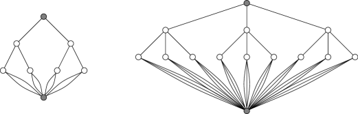
Figure 1: $G_{3}^{2}$ is a complete binary tree of height three with all leaves identified, and $G^{3}_{3}$ is a complete ternary tree of height three with all leaves identified.

We consider $G_{n}^{r}$ as a 2-terminal graph in which the terminals are the root and the identified-leaves vertex. It is easy to see that $G_{n}^{r}$ is in fact 2-terminal series-parallel, as it can be defined recursively as follows:

$$G_{1}^{r}&=K_{2}^{(r)}\\ G_{n+1}^{r}=(K_{2}\mathbin{\bowtie}G_{n}^{r})^{\mathbin{\|}r}$$ (3.7)

where $K_{2}^{(r)}$ is the graph with two vertices connected by $r$ parallel edges, and $G^{\mathbin{\|}r}$ denotes the parallel composition of $r$ copies of $G$. It then follows that $G_{n}^{r}$ has $(r^{n}+r-2)/(r-1)$ vertices, that the flow between its terminals is $r$ (for $n\geq 1$), and that its maxmaxflow is $r+1$ (for $n\geq 2$).

In Appendix B we shall prove the following:

Theorem 3.11

For fixed $r\geq 2$, every point of the circle $|q-1|=r$ is a limit point of chromatic roots for the family $\{G_{n}^{r}\}_{n\geq 1}$ of leaf-joined trees of branching factor $r$. [More precisely, for every $q_{0}$ satisfying $|q_{0}-1|=r$ and every $\epsilon>0$, there exists $n_{0}=n_{0}(q_{0},\epsilon)$ such that for all $n\geq n_{0}$ the graph $G_{n}^{r}$ has a chromatic root $q$ lying in the disc $|q-q_{0}|<\epsilon$.]

4 An abstract theorem on excluding roots

The multivariate Tutte polynomial of the graph $G=K_{2}$ having a single non-loop edge of weight $v_{e}$ is $Z_{K_{2}}(q,{\bf v})=q(q+v_{e})$, which has roots at $q=0$ and $q=-v_{e}$. Given a 2-terminal series-parallel graph $G$ with arbitrary complex edge weights $\{v_{e}\}$ and a fixed complex number $q$, we can apply series and parallel reductions as in Section 3.4 until $G$ has been reduced to a single edge with some “effective weight” $v_{\rm eff}\in{\mathbb{C}}\cup\{\hbox{undefined}\}$. If $v_{\rm eff}\neq\hbox{undefined}$, then we can be sure that none of the prefactors of the form $q+v_{e_{1}}+v_{e_{2}}$ generated during the series reductions were 0, and we can therefore conclude that $Z_{G}(q,{\bf v})=0$ if and only if $q=0$ or $v_{\rm eff}=-q$.

This observation then gives us a strategy for determining root-free regions for the multivariate Tutte polynomials of families of series-parallel graphs. For a fixed $q\neq 0$ in the conjectured root-free region, we bound the regions of the (finite) complex $v$-plane where $v_{\rm eff}$ can lie for any graph in the family, and we show that these regions do not contain the point $v_{\rm eff}=-q$ that would correspond to a zero of $Z_{G}(q,{\bf v})$. If we can do this, then we have shown that $Z_{G}(q,{\bf v})\neq 0$. The precise result is as follows:

Theorem 4.1

Let $q\neq 0$ be a fixed complex number and let $\Lambda\geq 2$ be a fixed integer. Let $S_{1}\subseteq S_{2}\subseteq\cdots\subseteq S_{\Lambda-1}$ be sets in the (finite) complex $v$-plane such that

• $S_{k}\mathbin{\bowtie^{V}_{q}}S_{\ell}\subseteq S_{\min(k,\ell)}$ for all $k,\ell$

• $S_{k}\mathbin{\|^{V}}S_{\ell}\subseteq S_{k+\ell}$ for $k+\ell\leq\Lambda-1$

Now consider any 2-terminal series-parallel graph $(G,s,t)$ and any maximal decomposition tree for $(G,s,t)$ in which all the proper constituents have between-terminals flow at most $\Lambda-1$, and equip $G$ with edge weights $v_{e}\in S_{1}$. Then, for every node $(H,a,b)$ of the decomposition tree that has between-terminals flow $\lambda_{H}(a,b)\leq\Lambda-1$, we have $v_{\rm eff}(H,a,b)\in S_{\lambda_{H}(a,b)}$.

Now assume further that, in addition to (1) and (2), the following hypotheses hold:

• $-q\notin S_{\Lambda-1}$

• $-q\notin S_{k}\mathbin{\|^{V}}S_{\ell}$ for $k+\ell=\Lambda$

Then, for any loopless series-parallel graph $G$ with maxmaxflow at most $\Lambda$, we have $Z_{G}(q,{\bf v})\not=0$ whenever $v_{e}\in S_{1}$ for all edges. (In particular, if $-1\in S_{1}$, then $q$ is not a chromatic root of $G$.)

Remarks. 1. It is implicit in condition (1) that the operation in question is always well-defined (i.e. does not take the value “undefined”), or in other words that $q+v_{1}+v_{2}\neq 0$ whenever $v_{1}\in S_{k}$ and $v_{2}\in S_{\ell}$.

2. When the root of the decomposition tree is a $p$-node (which occurs in particular whenever $G$ is nonseparable and not $K_{2}$) and $G$ has maxmaxflow $\Lambda$, then Lemma 3.9 guarantees that every proper constituent has between-terminals flow at most $\Lambda-1$. The root node $(G,s,t)$, by contrast, might have between-terminals flow as large as $\Lambda$.  $\Box$

Proof.  Let $(G,s,t)$, its maximal decomposition tree and its edge weights be as specified. We want to prove that $v_{\rm eff}(H,a,b)\in S_{\lambda_{H}(a,b)}$ for all nodes $(H,a,b)$ that satisfy $\lambda_{H}(a,b)\leq\Lambda-1$. We shall prove this claim by induction upwards from the leaves of the decomposition tree. By Lemma 3.8, a leaf of the decomposition tree is an edge $e$ of $G$, hence has between-terminals flow equal to 1, and $v_{\rm eff}=v_{e}\in S_{1}$ by hypothesis. So let $(H,a,b)$ be a non-leaf node of the decomposition tree and suppose that the children of $(H,a,b)$, call them $(H_{1},a_{1},b_{1})$ and $(H_{2},a_{2},b_{2})$, have between-terminals flow $k$ and $\ell$, respectively. Since $(H_{1},a_{1},b_{1})$ and $(H_{2},a_{2},b_{2})$ are proper constituents, we have by hypothesis $k,\ell\leq\Lambda-1$; so by the inductive hypothesis, we have $v_{\rm eff}(H_{1},a_{1},b_{1})\in S_{k}$ and $v_{\rm eff}(H_{2},a_{2},b_{2})\in S_{\ell}$. Using Lemma 3.5, it is clear that conditions (1) and (2) ensure that $v_{\rm eff}(H,a,b)\in S_{\lambda_{H}(a,b)}$ holds whenever $\lambda_{H}(a,b)\leq\Lambda-1$ (which holds for all proper constituents and might or might not hold for the root node). This proves the first half of the theorem.

As $Z_{G}(q,{\bf v})$ is multiplicative over blocks, and the maxmaxflow of a separable graph is the maximum of the maxmaxflows of its blocks, it suffices to prove the second half of the theorem when $G$ is a loopless nonseparable series-parallel graph of maxmaxflow at most $\Lambda$. Since the result holds trivially when $G=K_{1}$, we can assume that $G$ has at least one edge. Therefore, by Theorem 3.3, $G$ has a pair of vertices $s$, $t$ such that $(G,s,t)$ is a 2-terminal series-parallel graph and hence described by a maximal decomposition tree whose leaf nodes are single edges. Furthermore, by Lemma 3.9, all of the proper constituents of $(G,s,t)$ have between-terminals flow at most $\Lambda-1$. Therefore, if $(H,a,b)$ is a proper constituent of $(G,s,t)$ with between-terminals flow $\lambda_{H}(a,b)=\lambda$, we can apply the first half of the theorem to conclude that $v_{\rm eff}(H,a,b)\in S_{\lambda}$.

By condition (3) [and the nesting $S_{i}\subseteq S_{\Lambda-1}$], we have $v_{\rm eff}(H,a,b)\neq-q$ whenever $(H,a,b)$ is a proper constituent of $(G,s,t)$. On the other hand, the final step (at the root of the decomposition tree) constructs $(G,s,t)$ as the parallel composition of two proper constituents whose between-terminal flows sum to $\lambda_{G}(s,t)\leq\Lambda$, so conditions (4) and (2)/(3) together ensure that $v_{\rm eff}(G,s,t)\neq-q$. Therefore, by Algorithm 2 of Section 3.4, $Z_{G}(q,{\bf v})$ is equal to a nonzero prefactor — namely, the product over $s$-nodes of $q+v_{\rm eff}(G_{1},s_{1},t_{1})+v_{\rm eff}(G_{2},s_{2},t_{2})$, a quantity that is nonvanishing by virtue of Remark 1 preceding this proof — multiplied by $q[q+v_{\rm eff}(G,s,t)]$, and is therefore nonzero as claimed.  $\Box$

Of course, to apply this theorem it is necessary to actually identify suitable sets $S_{1}\subseteq S_{2}\subseteq\ldots\subseteq S_{\Lambda-1}$. In practice one usually starts from a specified set ${\mathcal{V}}\subseteq{\mathbb{C}}$ of “allowed edge weights” — for instance, ${\mathcal{V}}=\{-1\}$ for the chromatic polynomial — and one attempts to find sets $S_{1}\subseteq S_{2}\subseteq\ldots\subseteq S_{\Lambda-1}$ satisfying $S_{1}\supseteq{\mathcal{V}}$ along with the hypotheses (1)–(4) of Theorem 4.1. For any particular combination of $q$, $\Lambda$ and ${\mathcal{V}}$, there is always a collection of minimal regions $S_{1}\subseteq S_{2}\subseteq\ldots\subseteq S_{\Lambda-1}$ where $S_{1}\supseteq{\mathcal{V}}$ and conditions (1) and (2) are satisfied. If one knows this collection of minimal regions, then conditions (3) and (4) become a “final check” certifying that $q$ is not a root.

In practice, though, it is almost always impossible to describe the minimal regions even for specific values of $q$ and $\Lambda$, let alone symbolically (but see Section 5 for some computer-generated approximations). Therefore it is necessary to bound the optimal regions inside larger regions with shapes that are more amenable to analysis. But it is also important to fit the bounding regions as tightly as possible to the optimal regions, as conditions (1) and (2) cause any “unnecessary points” included in the approximation to a region to have a cascading effect on the approximations for the other regions, thereby incorporating still more possibly unnecessary points, and so on.

There are, in fact, two slightly different reasons why including unnecessary points in the regions $S_{i}$ can lead to poor bounds. Firstly, if we have chosen $S_{2},S_{3},\ldots$ to be much larger than they need to be, for the given set $S_{1}$, then the bounds one obtains from Theorem 4.1 may (not surprisingly) be much weaker than the truth. Secondly, it is important to observe that even if we are ultimately interested in proving $Z_{G}(q,{\bf v})\neq 0$ for weights $v_{e}$ lying in a specified set ${\mathcal{V}}$, we will get from Theorem 4.1, whether we like it or not, the same result for all $v_{e}\in S_{1}$. Of course, if $S_{1}$ is exactly the minimal region containing the given ${\mathcal{V}}$ and satisfying conditions (1) and (2), then nothing is lost, as any bound valid for all series-parallel graphs of maxmaxflow $\Lambda$ with weights in ${\mathcal{V}}$ will also be valid for weights in $S_{1}$ (since any $v$ lying in the minimal region $S_{1}$ is in fact the $v_{\rm eff}$ for a suitable 2-terminal series-parallel graph of maxmaxflow $\Lambda$ and between-terminals flow 1, with edge weights in ${\mathcal{V}}$). But if the chosen $S_{1}$ is significantly larger than the minimal region, then even the best-possible bound for weights in $S_{1}$ may be much weaker than the corresponding bound for weights in ${\mathcal{V}}$. In particular, if $S_{1}$ extends much outside the “complex antiferromagnetic regime” $|1+v_{e}|\leq 1$ — where “much outside” means, roughly, more than a distance of order $1/|q|$ — then one expects the $q$-plane roots of $Z_{G}(q,{\bf v})$ to grow exponentially in $\Lambda$ rather than linearly (see [27] for further discussion, and see also footnote 19 below).

The simplest types of region to manipulate analytically are discs, especially discs centered at the origin, and so it is natural to try to bound the optimal regions inside suitable discs. If one insists on using discs centered at the origin, then it furthermore matters whether one uses the $v$-variables, the $y$-variables or the $t$-variables. If one makes a poor choice — e.g. the optimal regions are either far from being discs, or far from being centered at the origin in the chosen variables — then one will obtain poor bounds, e.g. bounds that grow exponentially rather than linearly in $\Lambda$.

It turns out that the optimal regions are not too far from being discs centered at the origin if we use the $t$-variables, but are quite far from being discs centered at the origin if we use the $v$- or $y$-variables. We shall therefore use the $t$-variables in the remainder of this paper. Let us recall that the important points $v=-1$, $v=\infty$ and $v=-q$ correspond to $t=1/(1-q)$, $t=1$ and $t=\infty$, respectively. We can therefore re-express Theorem 4.1 in the language of transmissivities $\{t_{e}\}$. For simplicity we suppress the statements about $v_{\rm eff}$ (or $t_{\rm eff}$) and concentrate on the conclusion that $Z_{G}(q,{\bf v})\neq 0$.

Theorem 4.2

Let $q\not=0$ be a fixed complex number and let $\Lambda\geq 2$ be a fixed integer. Let $S_{1}\subseteq S_{2}\subseteq\cdots\subseteq S_{\Lambda-1}$ be sets in the (finite) complex $t$-plane such that

• $S_{k}\mathbin{\bowtie^{T}}S_{\ell}\subseteq S_{\min(k,\ell)}$ for all $k,\ell$

• $S_{k}\mathbin{\|^{T}_{q}}S_{\ell}\subseteq S_{k+\ell}$ for $k+\ell\leq\Lambda-1$

• $1\notin S_{\Lambda-1}$

• $S_{k}\mathbin{\|^{T}_{q}}S_{\ell}\subseteq{\mathbb{C}}$ for $k+\ell=\Lambda$ (i.e. does not ever take the value “undefined”)

Then, for any series-parallel graph $G$ with maxmaxflow at most $\Lambda$, we have $Z_{G}(q,{\bf v})\not=0$ whenever $v_{e}/(q+v_{e})\in S_{1}$ for all edges.

In particular, to handle chromatic polynomials it suffices to arrange that $1/(1-q)\in S_{1}$.

Remark. Condition (3) states merely that the set $S_{\Lambda-1}$ avoids the point $t=1$, but in practice we will always have $S_{\Lambda-1}\subseteq\{|t|<1\}$. Indeed, if $S_{\Lambda-1}$ contains any point with $|t|=1$ (resp. $|t|>1$), then by condition (1) its closure $\overline{S}_{\Lambda-1}$ must contain the point $t=1$ (resp. $t=\infty$); and while this is not explicitly forbidden, it is hard to see how one could satisfy all the hypotheses (1)–(4) in such a case.

Proof of Theorem 4.2.  This is almost a direct translation of Theorem 4.1 into transmissivities. Indeed, conditions (1) and (2) here are direct translations of conditions (1) and (2) of Theorem 4.1. Condition (3^′) here is equivalent to the hypothesis in Theorem 4.1 that the sets lie in the finite $v$-plane, while condition (3) of Theorem 4.1 is equivalent to the hypothesis here that the sets lie in the finite $t$-plane. Finally, condition (4) here is a direct translation of condition (4) of Theorem 4.1.  $\Box$

Since the regions $S_{i}$ are assumed increasing, the condition (1) is most stringent for $\ell=\Lambda-1$, and it reduces to

• $S_{k}\mathbin{\bowtie^{T}}S_{\Lambda-1}\subseteq S_{k}$  for all $k$.

Furthermore, there is a simple but very useful sufficient condition for condition (1)/(1^′) to hold:

Lemma 4.3

If there exists $r>0$ such that

$$D(r^{2})\subseteq S_{1}\subseteq S_{2}\subseteq\cdots\subseteq S_{\Lambda-1}\subseteq D(r)$$ (4.1)

where $D(r)=\{t\in{\mathbb{C}}\colon\,|t|\leq r\}$, then condition (1) of Theorem 4.2 holds.

Proof. $S_{k}\mathbin{\bowtie^{T}}S_{\ell}\subseteq D(r)\mathbin{\bowtie^{T}}D(r)=D(r^{2})\subseteq S_{\min(k,\ell)}$.  $\Box$

5 Discs in the $t$-plane

In this section we shall prove the following slight strengthening of Theorem 1.4:

Theorem 5.1

Fix an integer $\Lambda\geq 2$, and let $G$ be a loopless series-parallel graph of maxmaxflow at most $\Lambda$. Let $\rho^{\star}_{\Lambda}$ be the unique solution of

$$(1+\rho)^{\Lambda}\;=\;2(1+\rho^{2})^{\Lambda-1}$$ (5.1)

in the interval $(0,1)$ when $\Lambda\geq 3$, and let $\rho^{\star}_{2}=1$. Then the multivariate Tutte polynomial $Z_{G}(q,{\bf v})$ is nonvanishing whenever $|q-1|\geq 1/\rho^{\star}_{\Lambda}$ (with $\geq$ replaced by $>$ when $\Lambda=2$) and the edge weights ${\bf v}=\{v_{e}\}_{e\in E}$ satisfy

$$v_{e}\,=\,-1\quad\hbox{or}\quad\left|{v_{e}\over q+v_{e}}\right|\>\leq\>\rho\,{X-1\over 1-\rho X}$$ (5.2)

(again with strict inequality when $\Lambda=2$), where

$$\rho\>=\>{1\over|q-1|}\quad\hbox{and}\quad X\,=\,\biggl{(}{2\over 1+\rho}\biggr{)}^{1/(\Lambda-1)}\;.$$ (5.3)

Furthermore we have $\rho^{\star}_{\Lambda}>(\log 2)/(\Lambda-{\textstyle{3\over 2}}\log 2)$, so that in particular all the roots (real or complex) of the chromatic polynomial $P_{G}(q)$ lie in the disc $|q-1|<(\Lambda-{\textstyle{3\over 2}}\log 2)/\log 2$.

Remark. We shall see in Lemma 5.6 that under the hypothesis $|q-1|\geq 1/\rho^{\star}_{\Lambda}$ (i.e. $\rho\leq\rho^{\star}_{\Lambda}$) we have

$$\rho\,{X-1\over 1-\rho X}\;\geq\;\rho^{2}\;,$$ (5.4)

so that the conclusion of Theorem 5.1 holds under the more stringent but simpler condition

$$v_{e}\,=\,-1\quad\hbox{or}\quad\left|{v_{e}\over q+v_{e}}\right|\>\leq\>{1\over|q-1|^{2}}\;.$$ (5.5)

$\Box$

We shall prove Theorem 5.1 by exhibiting regions $S_{1}\subseteq S_{2}\subseteq\cdots\subseteq S_{\Lambda-1}$ of the complex $t$-plane that satisfy the conditions of Theorem 4.2 when $|q-1|\geq 1/\rho^{\star}_{\Lambda}$ and for which the set $S_{1}$ corresponds precisely to (5.2). Since in this section we shall always be working in the $t$-plane, we shall henceforth drop the superscripts ^T from the operators $\mathbin{\|^{T}_{q}}$ and $\mathbin{\bowtie^{T}}$. Let us also recall that, in the $t$-plane, series connection $\mathbin{\bowtie}$ is simply multiplication.

Before beginning this proof, it is instructive to engage in some informal motivation of our constructions.

If we want to handle the chromatic polynomial using Theorem 4.2, then we must certainly have $1/(1-q)\in S_{1}$. The set of minimal regions $S_{i}$ that contain the point $1/(1-q)$ and satisfy the first two conditions of Theorem 4.2 can be approximated by computer, because these conditions can be viewed as rules for constructing each $S_{i}$ from certain others. By imposing a fine grid on the disc $|t|<1$ and “rounding” each complex number to the closest grid point, we can restrict our attention to a finite number of points. We start by marking $t_{0}=1/(1-q)$ as belonging to $S_{1}$ (and hence to each $S_{i}$); we then iteratively construct approximations to the regions $S_{1},S_{2},\ldots,S_{\Lambda-1}$ by using conditions (1) and (2) of Theorem 4.2 until the approximations are closed under further application of the rules. If the resulting region $S_{\Lambda-1}$ is contained in the open unit disc $\{|t|<1\}$, then Theorem 4.2 implies that $q$ is not a chromatic root for any graph of maxmaxflow $\Lambda$.

Repeating these experiments for a range of different values of $q$ and moderate values of $\Lambda$ suggests that although the minimal regions are generally complicated shapes, they are often loosely “disc-like” and can be bounded reasonably well by a disc in the $t$-plane centered at the origin. Some examples with $\Lambda=3$ are shown in Figure 2, and a more extensive set of plots is included with the preprint version of this paper at arXiv.org.

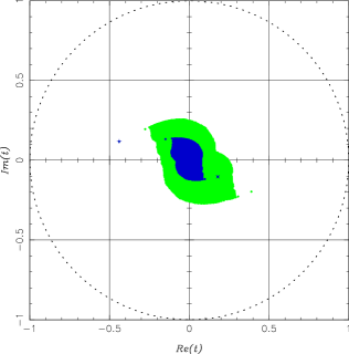
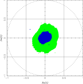
(a) $q=3.125+0.569i\approx 1+2.2e^{\pi i/12}$	(b) $q=2.905+1.100i\approx 1+2.2e^{\pi i/6}$
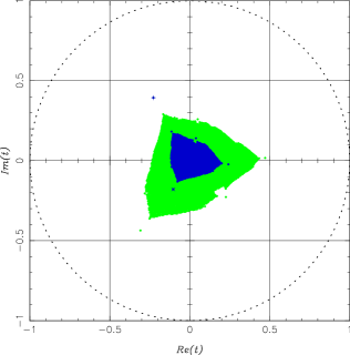
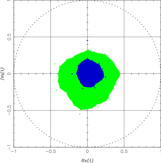
(c) $q=2.100+1.905i\approx 1+2.2e^{\pi i/3}$	(d) $q=1.000+2.200i\approx 1+2.2e^{\pi i/2}$
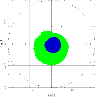
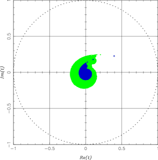
(e) $q=-0.100+1.905i\approx 1+2.2e^{2\pi i/3}$	(f) $q=-0.905+1.100\approx 1+2.2e^{5\pi i/6}$

Figure 2: Computer-generated approximations to $S_{1}$ (dark blue) and $S_{2}$ (light green) in the complex $t$-plane, for $\Lambda=3$ and selected values of $q$. Note that we always have $S_{1}\subseteq S_{2}$ and $S_{1}=\{t_{0}\}\cup t_{0}S_{2}$ where $t_{0}=1/(1-q)$. The points $t_{0}$ and $t_{0}\mathbin{\bowtie}t_{0}=t_{0}^{2}$, which both belong to $S_{1}$, are shown as dark blue $+$ and $\times$, respectively. The circle $|t|=1$ is shown for reference in dashed black.

In fact we need to be a bit more careful, because every region $S_{i}$ must contain the point $t_{0}=1/(1-q)$, but taking the smallest region $S_{1}$ to be a disc of radius $\rho=|t_{0}|=|1/(1-q)|$ cannot give very good bounds. Indeed, with this choice of $S_{1}$ there exist graphs $G$ of maxmaxflow $\Lambda$ having roots $Z_{G}(q,v)=0$ with $v\in S_{1}$ and $q$ growing exponentially in $\Lambda$ (more precisely like $2^{\Lambda}$).

However, a slight modification works: namely, we take each region $S_{i}$ to be a “point + disc”

$$S_{i}\;=\;\{1/(1-q)\}\cup D(r_{i})$$ (5.6)

where $D(r_{i})$ is a closed disc of radius $r_{i}$ centered at the origin. This choice results in a situation that is both amenable to analysis and also yields good bounds when the radii $r_{i}$ are suitably chosen, as we will prove in this section.

The disc $D(r_{1})$ must have radius at least $\rho^{2}$ because it must contain the point $t_{0}\mathbin{\bowtie}t_{0}=1/(1-q)^{2}$. So choose some $r_{1}\geq\rho^{2}$; this choice of $r_{1}$ sets a lower bound on the possible values for $r_{2}$ because $S_{1}\mathbin{\|_{q}}S_{1}\subseteq S_{2}$. Continuing in this fashion, $r_{1}$ and $r_{2}$ determine the minimum allowable value for $r_{3}$; then $r_{1}$, $r_{2}$ and $r_{3}$ determine the minimum allowable value for $r_{4}$; and so on. Ultimately this process determines a minimum allowable value for $r_{\Lambda-1}$; and if $r_{\Lambda-1}\leq\rho$, then the set of radii $r_{1},r_{2},\ldots,r_{\Lambda-1}$ yields a set of regions $S_{i}$ defined by (5.6) that satisfies the conditions of Theorem 4.2. We formalize this observation in the following proposition:

Proposition 5.2

Let $\Lambda\geq 2$ be a fixed integer; then let $q$ be a fixed complex number satisfying $|q-1|>1$, and set $t_{0}=1/(1-q)$ and $\rho=|t_{0}|$. If the real numbers $r_{1},r_{2},\ldots,r_{\Lambda-1}$ satisfy

$$\rho^{2}\leq r_{1}\leq r_{2}\leq\cdots\leq r_{\Lambda-1}\leq\rho$$ (5.7)

and

$$r_{s}\;\geq\;\max\{|t_{e}\mathbin{\|_{q}}t_{f}|\colon\;t_{e}\in D(r_{k}),\,t_{f}\in D(r_{\ell}),\,k+\ell=s\}$$ (5.8)

for $2\leq s\leq\Lambda-1$, then the set of regions $S_{1}$, $S_{2}$, $\ldots$, $S_{\Lambda-1}$ defined by

$$S_{i}\;=\;\{1/(1-q)\}\cup D(r_{i})$$ (5.9)

satisfies the conditions of Theorem 4.2.

Proof.  We need to show that the four conditions of Theorem 4.2 hold. Condition (1) holds by Lemma 4.3 with $r=\rho$. To check condition (2), we observe that

$$S_{k}\mathbin{\|_{q}}S_{\ell}\;=\;\left(\{t_{0}\}\cup D(r_{k})\right)\mathbin{\|_{q}}\left(\{t_{0}\}\cup D(r_{\ell})\right)\;=\;\{t_{0}\}\cup\left(D(r_{k})\mathbin{\|_{q}}D(r_{\ell})\right)$$ (5.10)

because $t_{0}\mathbin{\|_{q}}t=t_{0}$ for every $t$. Therefore condition (5.8) on the radii is exactly what is needed to ensure that $S_{k}\mathbin{\|_{q}}S_{\ell}\subseteq S_{k+\ell}$. Condition (3) holds because $S_{\Lambda-1}\subseteq D(\rho)$ and $\rho<1$. Finally, condition (4) fails only if there are $t_{e}\in S_{k}$ and $t_{f}\in S_{\ell}$ (with $k+\ell=\Lambda$, though we do not even need to use this constraint) such that $t_{e}t_{f}=1/(1-q)$, but this is impossible because $|t_{e}t_{f}|\leq\rho^{2}<\rho=1/|1-q|$.  $\Box$

To apply this theorem, we need to be able to bound the modulus of

$$t_{e}\mathbin{\|}_{q}t_{f}\;=\;\frac{t_{e}+t_{f}+(q-2)t_{e}t_{f}}{1+(q-1)t_{e}t_{f}}$$ (5.11)

when $t_{e}\in D(r_{k})$ and $t_{f}\in D(r_{\ell})$. Since the maximum modulus of $t_{e}\mathbin{\|_{q}}t_{f}$ occurs when $t_{e}$ and $t_{f}$ are on the boundaries of their respective discs, let us define for $x,y\in[0,\rho)$ the function

$$f_{q}(x,y)\;:=\;\max\{|t_{e}\mathbin{\|_{q}}t_{f}|\,\colon\;|t_{e}|=x,\,|t_{f}|=y\}\;.$$ (5.12)

If we bound (5.11) in the most naive way by replacing the numerator by an upper bound and the denominator by a lower bound, and we furthermore use $|q-2|\leq|q-1|+1$ to express the $q$-dependence in terms of the single number $|q-1|$, then we get

$$f_{q}(x,y)\;\leq\;F_{q}(x,y)\;:=\;\frac{x+y+(|q-1|+1)xy}{1-|q-1|xy}\;=\;\frac{x+y+(\rho^{-1}+1)xy}{1-\rho^{-1}xy}\;.$$ (5.13)

The condition $x,y\in[0,\rho)$ ensures that the denominator of $F_{q}(x,y)$ is strictly positive. Therefore, given the chosen value of $r_{1}$, we can define a sequence of radii $r_{2},r_{3},\ldots$ satisfying (5.8) using the iteration

$$r_{s}\;=\;\max\{F_{q}(r_{k},r_{\ell})\colon\;k+\ell=s\}$$ (5.14)

(stopping the iteration whenever a result $r_{s}$ becomes $\geq\rho$). It is immediate that $r_{1}\leq r_{2}\leq\ldots\;$. If the iteration remains well-defined up to $s=\Lambda-1$ and satisfies $r_{\Lambda-1}\leq\rho$, then the radii satisfy the hypotheses of Proposition 5.2. (Henceforth let us write $F$ in place of $F_{q}$ to lighten the notation.)

At first sight, this seems rather unappealing for analysis because the $\max$ in (5.14) appears difficult to handle. However, this difficulty is illusory because it turns out that $F$ is actually an associative function:

Lemma 5.3

Let $G$ be a function of the form

$$G(x,y)\;=\;\frac{x+y+Axy}{1+Bxy}$$ (5.15)

where $A$, $B$ are arbitrary constants. Then

$$G(x,G(y,z))\;=\;G(y,G(x,z))\;=\;G(z,G(x,y))\;.$$ (5.16)

Proof.  Direct calculation shows that

$$G(x,G(y,z))\;=\;\frac{(x+y+z)+A(xy+yz+xz)+(A^{2}+B)xyz}{1+B(xy+xz+yz)+ABxyz}\;,$$ (5.17)

which is clearly symmetric under all permutations of $\{x,y,z\}$.  $\Box$

Corollary 5.4

If $F$ is given by (5.13) and $r_{2},\ldots,r_{\Lambda-1}$ by (5.14), then

$$F(r_{k},r_{\ell})\;=\;F(r_{1},r_{k+\ell-1})$$ (5.18)

for all pairs $k,\ell$ of positive integers such that $k+\ell\leq\Lambda$.

Proof.  We prove this by induction on $s=k+\ell$. The result clearly holds for $s=2$. So suppose that the result is true for all $k^{\prime}+\ell^{\prime}<k+\ell$. Then

$$F(r_{k},r_{\ell})=F(F(r_{1},r_{k-1}),r_{\ell})=F(r_{1},F(r_{k-1},r_{\ell}))=F(r_{1},r_{k+\ell-1})$$ (5.19)

and the result holds.  $\Box$

The key point of this lemma (which was used implicitly in the proof) is that all the terms in (5.14) are actually the same, and so we can arbitrarily choose any one of them to define $r_{s}$. So let us take $r_{s+1}=F(r_{1},r_{s})$, i.e.

$$r_{s+1}\;=\;\frac{[1+(\rho^{-1}+1)r_{1}]r_{s}+r_{1}}{1-\rho^{-1}r_{1}r_{s}}\;.$$ (5.20)

Since the map $r_{s}\mapsto r_{s+1}$ is a Möbius transformation, we can obtain an explicit expression for $r_{k}$:

Lemma 5.5

For fixed real numbers $r_{1}$ and $\rho\neq 1$, define a sequence $r_{1},r_{2},\ldots\in{\mathbb{R}}\cup\{\infty\}$ by

$$r_{s+1}\;=\;\frac{[1+(\rho^{-1}+1)r_{1}]r_{s}+r_{1}}{1-\rho^{-1}r_{1}r_{s}}\;.$$ (5.21)

Then

$$r_{k}\;=\;\rho\,\frac{(1+r_{1}/\rho)^{k}-(1+r_{1})^{k}}{(1+r_{1})^{k}-\rho(1+r_{1}/\rho)^{k}}\;.$$ (5.22)

Proof.  The map $r_{s}\mapsto r_{s+1}$ is a (real) Möbius transformation of the form

$$x\;\mapsto\;\frac{ax+b}{cx+d}$$ (5.23)

whose coefficients can be displayed in a suitable matrix

$$M\,=\,\left(\begin{array}[]{cc}a&b\\ c&d\end{array}\right)\,=\,\left(\begin{array}[]{cc}1+(\rho^{-1}+1)r_{1}&r_{1}\\ -\rho^{-1}r_{1}&1\end{array}\right)\,.$$ (5.24)

By standard results on Möbius transformations, the matrix $M^{k}$ represents the $k$th iterate of this transformation. Now, the matrix $M$ has eigenvalues $1+r_{1}/\rho$ and $1+r_{1}$, and it can be diagonalized by $M=QDQ^{-1}$ where

$$D = \left(\begin{array}[]{cc}1+r_{1}/\rho&0\\ 0&1+r_{1}\end{array}\right)$$ (5.27)

$$Q = \frac{1}{1-\rho}\left(\begin{array}[]{cc}1&-\rho\\ -1&1\end{array}\right)$$ (5.30)

$$Q^{-1} = \left(\begin{array}[]{cc}1&\rho\\ 1&1\end{array}\right)$$ (5.33)

It follows immediately that $M^{k}=QD^{k}Q^{-1}$ and so

$$M^{k}\;=\;\frac{1}{1-\rho}\left(\begin{array}[]{cc}(1+r_{1}/\rho)^{k}-\rho(1+r_{1})^{k}&\rho[(1+r_{1}/\rho)^{k}-(1+r_{1})^{k}]\\[5.69054pt] (1+r_{1})^{k}-(1+r_{1}/\rho)^{k}&(1+r_{1})^{k}-\rho(1+r_{1}/\rho)^{k}\\ \end{array}\right).$$ (5.34)

Treating this as a Möbius transformation and applying it to $r_{0}=0$, we get $r_{k}=(M^{k})_{12}/(M^{k})_{22}$ and thus

$$r_{k}\;=\;\rho\,\frac{(1+r_{1}/\rho)^{k}-(1+r_{1})^{k}}{(1+r_{1})^{k}-\rho(1+r_{1}/\rho)^{k}}\;.$$ (5.35)

This also reproduces the correct value at $k=1$.  $\Box$

Remarks. 1. The formula (5.22), once we have it, can of course be proven by an easy induction on $k$. But we thought it preferable to give a more conceptual proof that shows where (5.22) comes from. Note also that we can rewrite (5.22) as

$$r_{k}\>=\>\rho\,\frac{X^{k}-1}{1-\rho X^{k}}\quad\text{where}\quad X\>=\>\frac{1+r_{1}/\rho}{1+r_{1}}\;;$$ (5.36)

this will be useful later.

2. The reasoning in Lemma 5.3, Corollary 5.4 and Lemma 5.5 can be made even more explicit by observing that the associative function $G(x,y)=(x+y+Axy)/(1+Bxy)$ is actually conjugate to $\widehat{G}(X,Y)=XY$: it suffices to make the Möbius change of variables $X=f(x):=(1+\alpha x)/(1+\beta x)$ with

$$\alpha&={A\pm\sqrt{A^{2}+4B}\over 2}\\ \beta={A\mp\sqrt{A^{2}+4B}\over 2}$$ (5.37)

and we then have

$$f\Big{(}G\big{(}f^{-1}(X),\,f^{-1}(Y)\big{)}\Big{)}\;=\;XY\;.$$ (5.38)

In our application we have $A=1+\rho^{-1}$ and $B=-\rho^{-1}$, hence $\alpha=\rho^{-1}$ and $\beta=1$ (or the reverse). Therefore, defining $R_{k}=f(r_{k}):=(1+\rho^{-1}r_{k})/(1+r_{k})$, we have simply $R_{k}=R_{1}^{k}$, which is equivalent to (5.22). Further information on associative rational functions in two variables can be found in [17].  $\Box$

The final step in proving Theorem 5.1 is to show that, for suitable $q$, we can choose $r_{1}\geq\rho^{2}$ and have $r_{k}\leq\rho$ for $1\leq k\leq\Lambda-1$. Whenever this is the case, the radii $r_{1},r_{2},\ldots,r_{\Lambda-1}$ defined by (5.21)/(5.22) will satisfy the conditions of Proposition 5.2, and hence the set of nested “point + disc” regions $S_{i}$ will satisfy the conditions of Theorem 4.2, thereby certifying that $Z_{G}(q,{\bf v})\neq 0$ whenever $G$ is a series-parallel graph of maxmaxflow at most $\Lambda$ and $v_{e}/(q+v_{e})\in S_{1}$ for all edges $e$.

The simplest choice is to take $r_{1}=\rho^{2}$ exactly; then from (5.22) we have

$$r_{k}\;=\;\rho\,\frac{X^{k}-1}{1-\rho X^{k}}\quad\text{where}\quad X\>=\>\frac{1+\rho}{1+\rho^{2}}\;.$$ (5.39)

When this choice works (i.e. satisfies $r_{k}\leq\rho$ for $1\leq k\leq\Lambda-1$), it yields the minimal regions $S_{i}$ of the form (5.9) that satisfy the conditions of Proposition 5.2. However, a slightly better choice is to take $r_{\Lambda-1}=\rho$ exactly; simple algebra using (5.22) then shows that

$$r_{k}\;=\;\rho\,\frac{X^{k}-1}{1-\rho X^{k}}\quad\hbox{where}\quad X\,=\,\biggl{(}{2\over 1+\rho}\biggr{)}^{1/(\Lambda-1)}\;.$$ (5.40)

When this choice works (i.e. satisfies $\rho^{2}\leq r_{k}\leq\rho$ for $1\leq k\leq\Lambda-1$), it yields the maximal regions $S_{i}$ of the form (5.9) that satisfy the conditions of Proposition 5.2, and hence the largest allowed set $S_{1}$ of edge weights. The following lemma shows that these two choices work in precisely the same set of circumstances, namely when $\rho\leq\rho^{\star}_{\Lambda}$ where $\rho^{\star}_{\Lambda}$ is defined by (5.1)/(5.41). In the borderline case $\rho=\rho^{\star}_{\Lambda}$ both choices yield the same sequence, which satisfies both $r_{1}=\rho^{2}$ and $r_{\Lambda-1}=\rho$. But when $\rho<\rho^{\star}_{\Lambda}$ we get different sequences, and we prefer to use the second choice because it yields a larger region $S_{1}$.

Lemma 5.6

For $\rho\in(0,1)$ and integer $\Lambda\geq 2$, the following are equivalent:

• There exist real numbers $r_{1},\ldots,r_{\Lambda-1}$ satisfying (5.21) and $\rho^{2}\leq r_{1}\leq\ldots\leq r_{\Lambda-1}\leq\rho$.

• The sequence defined by (5.39) satisfies $\rho^{2}\leq r_{k}\leq\rho$ for $1\leq k\leq\Lambda-1$.

• The sequence defined by (5.40) satisfies $\rho^{2}\leq r_{k}\leq\rho$ for $1\leq k\leq\Lambda-1$.

• $(1+\rho)^{\Lambda}\>\leq\>2(1+\rho^{2})^{\Lambda-1}$.

• $\rho\leq\rho^{\star}_{\Lambda}$, where $\rho^{\star}_{\Lambda}$ is the unique solution of

  $$(1+\rho)^{\Lambda}\;=\;2(1+\rho^{2})^{\Lambda-1}$$ (5.41)

  in the interval $(0,1)$ when $\Lambda\geq 3$, and $\rho^{\star}_{2}=1$.

Let us remark that the equation (5.41) has $\rho=1$ as a root, so that after division by $\rho-1$ it reduces to a polynomial equation of degree $2\Lambda-3$.

Proof of Lemma 5.6.  Fix $\rho\in(0,1)$ and $r_{1}>0$ and define a sequence $r_{1},r_{2},\ldots,r_{\Lambda-1}$ by (5.21)/(5.22); or equivalently, fix $\rho\in(0,1)$ and $X>1$ and define $r_{1},r_{2},\ldots,r_{\Lambda-1}$ by (5.36). It is then easy to see that we have $r_{1}\leq r_{2}\leq\ldots\leq r_{\Lambda-1}<\infty$ if and only if $X<\rho^{-1/(\Lambda-1)}$ [so that the denominator in the expression (5.36) for $r_{k}$ is positive for all $k\leq\Lambda-1$]; and each $r_{k}$ is an increasing function of $X$ (for fixed $\rho$) in the region $1<X<\rho^{-1/(\Lambda-1)}$. If we furthermore want to have $r_{1}\geq\rho^{2}$ and $r_{\Lambda-1}\leq\rho$, then we must have

$$\frac{1+\rho}{1+\rho^{2}}\;\leq\;X\;\leq\;\biggl{(}{2\over 1+\rho}\biggr{)}^{1/(\Lambda-1)}$$ (5.42)

(note that $[2/(1+\rho)]^{1/(\Lambda-1)}<\rho^{-1/(\Lambda-1)}$); and by the just-observed monotonicity in $X$, this condition is necessary and sufficient. This proves the equivalence of (a), (b) and (c). Moreover, there exists such an $X$ if and only if

$$\frac{1+\rho}{1+\rho^{2}}\;\leq\;\biggl{(}{2\over 1+\rho}\biggr{)}^{1/(\Lambda-1)}\;,$$ (5.43)

which is equivalent to (d). So (a)–(d) are all equivalent.

Finally we shall prove the equivalence of (d) and (e). We do this in slightly greater generality than is claimed, namely for all real $\Lambda\geq 2$. Consider the function

$$f_{\Lambda}(\rho)\;=\;\Lambda\log(1+\rho)\,-\,(\Lambda-1)\log(1+\rho^{2})\;.$$ (5.44)

Clearly (d) holds if and only if $f_{\Lambda}(\rho)\leq\log 2$. Now the first two derivatives of $f_{\Lambda}(\rho)$ are

$$f^{\prime}_{\Lambda}(\rho)&={\Lambda\over 1+\rho}\,-\,{2(\Lambda-1)\rho\over 1+\rho^{2}}\\ f^{\prime\prime}_{\Lambda}(\rho)=-\,{4(1+\rho+\rho^{2}-\rho^{3})\,+\,(\Lambda-2)(3+4\rho+2\rho^{2}-4\rho^{3}-\rho^{4})\over(1+\rho)^{2}(1+\rho^{2})^{2}}$$ (5.45)

For $0\leq\rho\leq 1$ we manifestly have $1+\rho+\rho^{2}-\rho^{3}\geq 1+\rho\geq 1$ and $3+4\rho+2\rho^{2}-4\rho^{3}-\rho^{4}\geq 3+\rho^{2}\geq 3$, so that $f_{\Lambda}$ is strictly concave on $[0,1]$ whenever $\Lambda\geq 2$. We have $f_{\Lambda}(0)=0$, $f^{\prime}_{\Lambda}(0)=\Lambda>0$, $f_{\Lambda}(1)=\log 2$ and $f^{\prime}_{\Lambda}(1)=-(\Lambda-2)/2$. Therefore, for $\Lambda>2$, there is a unique $\rho^{\star}_{\Lambda}\in(0,1)$ satisfying $f_{\Lambda}(\rho^{\star}_{\Lambda})=\log 2$; and for $\rho\in[0,1)$ we have $f_{\Lambda}(\rho)\leq\log 2$ if and only if $\rho\leq\rho^{\star}_{\Lambda}$. This proves the equivalence of (d) and (e) for all real $\Lambda>2$. When $\Lambda=2$, (d) holds for all $\rho\in[0,1]$, so (d) is again equivalent to (e) with $\rho^{\star}_{2}=1$.  $\Box$

We have now completed the proof of the main part of Theorem 5.1. All that remains is to prove the final statement that $\rho^{\star}_{\Lambda}>(\log 2)/(\Lambda-{\textstyle{3\over 2}}\log 2)$ for all integers $\Lambda\geq 2$, or equivalently (in view of Lemma 5.6d,e) that $(1+\rho)^{\Lambda}<2(1+\rho^{2})^{\Lambda-1}$ when $\rho=(\log 2)/(\Lambda-{\textstyle{3\over 2}}\log 2)$. We shall actually prove this for all real $\Lambda>{\textstyle{5\over 2}}\log 2\approx 1.732868$ (this ensures that $\rho<1$). Taking the logarithm of $2(1+\rho^{2})^{\Lambda-1}/(1+\rho)^{\Lambda}$, substituting for $\Lambda$ in terms of $\rho$, and parametrizing by $\rho\in(0,1)$, we see that this is equivalent to the following claim:

Lemma 5.7

The function

$$g(\rho)&=\rho\left[\log 2\>+\>\biggl{(}{\log 2\over\rho}\,+\,{\textstyle{3\over 2}}\log 2\,-\,1\biggr{)}\,\log(1+\rho^{2})\>-\>\biggl{(}{\log 2\over\rho}+{\textstyle{3\over 2}}\log 2\biggr{)}\,\log(1+\rho)\right]\\ \\ =\rho\log\left(\frac{2}{1+\rho}\right)\,-\,(\log 2)\log\left(\frac{1+\rho}{1+\rho^{2}}\right)\,-\,({\textstyle{3\over 2}}\log 2\,-\,1)\,\rho\,\log\left({1+\rho\over 1+\rho^{2}}\right)$$ (5.46)

is strictly positive for $0<\rho<1$.

Proof.  The second derivative of $g$ is given by $g^{\prime\prime}(\rho)=h(\rho)\times\rho/[(1+\rho)^{2}(1+\rho^{2})^{2}]$ where

$$h(\rho)\;=\;-(2-{\textstyle{3\over 2}}\log 2)\rho^{4}\,-\,(4-2\log 2)\rho^{3}\,-\,(8-5\log 2)\rho^{2}\,-\,(12-14\log 2)\rho\,+\,({\textstyle{23\over 2}}\log 2-6)\;.$$ (5.47)

All the coefficients of $h(\rho)$ are strictly negative except for the last (constant) term, so we have $h^{\prime}(\rho)<0$ for all $\rho\geq 0$. Since $h(0)={\textstyle{23\over 2}}\log 2-6>0$ and $h(1)=34\log 2-32<0$ and $h$ is strictly decreasing for $\rho\geq 0$, it follows that $h(\rho)$ has exactly one positive real root $\rho^{*}$ and that it lies between 0 and 1 (by computer $\rho^{*}\approx 0.417876$). Therefore $g$ is strictly convex on $[0,\rho^{*}]$ and strictly concave on $[\rho^{*},\infty)$. Since $g(0)=g^{\prime}(0)=0$, we have $g(\rho)>0$ for $\rho\in(0,\rho^{*}]$. Moreover, since $g(\rho^{*})>0$ and $g(1)=0$ and $g$ is strictly concave on $[\rho^{*},1]$, we have $g(\rho)>0$ for $\rho\in[\rho^{*},1)$. Hence $g(\rho)>0$ for all $\rho\in(0,1)$, as claimed.  $\Box$

Remark. A straightforward calculation shows that the large-$\Lambda$ asymptotic behavior of $\rho^{\star}_{\Lambda}$ is given by

$$\rho^{\star}_{\Lambda}\;=\;(\log 2)\Biggl{[}{1\over\Lambda-1}\,+\,{3\log 2-2\over 2(\Lambda-1)^{2}}\,+\,{25\log^{2}2-24\log 2+6\over 6(\Lambda-1)^{3}}\,+\,\ldots\Biggr{]}$$ (5.48)

and hence

$${1\over\rho^{\star}_{\Lambda}}\;=\;{\Lambda-1\over\log 2}\,-\,{3\log 2-2\over 2\log 2}\,-\,{23\log 2-12\over 12(\Lambda-1)}\,+\,\ldots\;\;.$$ (5.49)

So the inequality $\rho^{\star}_{\Lambda}>(\log 2)/(\Lambda-{\textstyle{3\over 2}}\log 2)$ captures the first two terms of the large-$\Lambda$ asymptotic behavior.  $\Box$

We have now completed the proof of Theorem 5.1.

6 The case $\Lambda=3$

Theorem 1.4 is a strong result because it provides a linear bound for the chromatic roots of series-parallel graphs in terms of the maxmaxflow $\Lambda$, thereby achieving our main objective. Furthermore, the constant $1/\log 2$ cannot be reduced below $1$ (see Appendix B) and so it is reasonably close to optimal. However, the result applies uniformly for all $\Lambda$, its proof involves a number of steps where expressions are replaced by fairly naive upper bounds, and it only involves the magnitude of $q-1$; so for all these reasons, Theorem 1.4 does not give a very precise picture of the root-free region for any particular value of $\Lambda$.

In this section we consider how to get sharper results for the simplest nontrivial case, namely for $\Lambda=3$. In this case, the bound given by Theorem 1.4 is that chromatic roots for series-parallel graphs of maxmaxflow 3 are contained in the disk

$$|q-1|\;\leq\;2/(\log 2)\;\approx\;2.8853900818\;.$$ (6.1)

An immediate improvement can be obtained from Theorem 5.1 by using the exact value of $\rho_{3}^{\star}$, which gives the slightly better bound

$$|q-1|\;\leq\;1/\rho_{3}^{\star}\;\approx\;2.6589670819\;.$$ (6.2)

Both of these regions ultimately relied on the quantity $F_{q}$ given by (5.13) as an upper bound for the true value $f_{q}$. We can do better by computing a numerical approximation to the actual value $f_{q}(\rho^{2},\rho^{2})$, and then imposing the condition $f_{q}(\rho^{2},\rho^{2})\leq\rho$ that arises out of Proposition 5.2 with $\Lambda=3$. Since $f_{q}(\rho^{2},\rho^{2})$ depends on $q$ and not just on $|q-1|$, this procedure will lead to a region with no simple analytic description. As $t_{e}\mathbin{\|_{q}}t_{f}$ is given by a ratio of symmetric multiaffine polynomials in $t_{e}$ and $t_{f}$ [cf. (5.11)] and $D(\rho^{2})$ is a circular region, the Grace–Walsh–Szegő coincidence theorem [36, Theorem 3.4.1b] implies that

$$\max_{t_{e},t_{f}\in D(\rho^{2})}|t_{e}\mathbin{\|_{q}}t_{f}|\;=\;\max_{t\in D(\rho^{2})}|t\mathbin{\|_{q}}t|\;,$$ (6.3)

and so we can compute an approximation to $f_{q}(\rho^{2},\rho^{2})$ by letting $t$ range over the (discretized) boundary of $D(\rho^{2})$ and taking the maximum value of $|t\mathbin{\|_{q}}t|$ thus obtained. Then for each fixed angle $\theta$ we can set $1/(1-q)=\rho e^{i\theta}$ and use the bisection method to determine the maximum possible value of $\rho$. Figure 3 shows how this bound (shown as a green solid curve) compares with the circular regions (6.1) and (6.2). This bound is the optimal bound obtainable from Theorem 4.2 under the assumption that $S_{1}$ is chosen to be a “point+disk” region $S_{1}=\{1/(1-q)\}\cup D(\rho^{2})$.

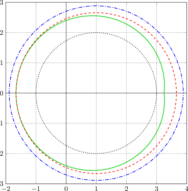
Figure 3: Different bounds on the chromatic roots for $\Lambda=3$: the bound based on $f_{q}$ (green solid curve), the bound $|q-1|=2.6589670819$ based on $F_{q}$ (red dashed circle), and the bound $|q-1|=2/\log 2\approx 2.8853900818$ from Theorem 1.4 (blue dot-dashed outer circle). The inner circle $|q-1|=2$ is also shown for reference (dotted gray).

At this point it is natural to inquire: What is the best possible result? Otherwise put: Can we describe exactly the closure of the set of all chromatic roots of all series-parallel graphs of maxmaxflow $\Lambda=3$, or at least the outer boundary of this set? In [38] one of the authors gave a computer approximation to this boundary, but he suspects that this approximation may become poor near the real axis, in part because this boundary is likely to be fractal-like rather than smooth.

As previously mentioned, we will show in Appendix B that, for each fixed $r\geq 2$, every point of the circle $|q-1|=r$ is a limit point (as $n\to\infty$) of chromatic roots of the family $\{G_{n}^{r}\}_{n\geq 1}$ of leaf-joined trees of branching factor $r$, which have maxmaxflow $\Lambda=r+1$. Moreover, numerical calculations suggest (though we have no proof) that the chromatic roots of leaf-joined trees always lie inside the circle $|q-1|=r$ (see Conjecture B.12). This led us to conjecture that the exact answer to our question is: the chromatic roots of series-parallel graphs of maxmaxflow $\Lambda$ always lie inside the disc $|q-1|<\Lambda-1$, and this bound is sharp.

That would be neat, but it is false! In fact, a counterexample can be found by a simple modification of a leaf-joined tree. Let us first recall [46, Example 2.2] the multivariate Tutte polynomial of a cycle $C$:

$$Z_{C}(q,{\bf v})\;=\;\prod_{e\in E(C)}(q+v_{e})\,+\,(q-1)\prod_{e\in E(C)}v_{e}\;.$$ (6.4)

In particular, if we consider a cycle of $N+1$ edges where $N$ edges carry weight $v$ and the last edge carries weight $-1$, we have

$$Z_{C}(q,{\bf v})\;=\;(q-1)[(q+v)^{N}-v^{N}]\;,$$ (6.5)

which vanishes whenever $t=v/(q+v)$ is an $N$th root of unity. It follows that if we consider any 2-terminal graph ${\sf G}=(G,s,t)$ and form the graph $H$ consisting of $N$ copies of ${\sf G}$ together with one $K_{2}$ connected in a cycle, then $H$ has a chromatic root whenever the “effective transmissivity” $t_{\rm eff}(G,s,t)$ is an $N$th root of unity.

It is easy to compute the effective transmissivity for leaf-joined trees, symbolically as a function of $q$, by using the recursion (B.11)/(B.12) along with $t=(y-1)/(q+y-1)$. We can then plot the curve in the complex $q$-plane where $|t_{\rm eff}(G_{n}^{r},s,t)|=1$. For $r=2$, we find that this curve stays within the disc $|q-1|<2$ when $n\leq 4$, but that it strays slightly outside this disc when $n=5$. (On the circle $q-1=2e^{i\theta}$, $|t_{\rm eff}(G_{5}^{2},s,t)|$ reaches a maximum value $\approx 1.08448$ at $\theta\approx\pm 0.679954\pi$, corresponding to $q\approx-0.071413\pm 1.68881i$.) If we now consider the graph $H$ consisting of $N=3$ copies of $G_{5}^{2}$ together with one $K_{2}$ connected in a cycle — note that $H$ has maxmaxflow 3 and has 94 vertices — we see that $H$ has a chromatic root whenever $t_{\rm eff}(G_{5}^{2},s,t)$ is a cube root of unity. Solving $t_{\rm eff}(G_{5}^{2},s,t)=e^{\pm 2\pi i/3}$ for $q$, we find 31 roots, of which one ($q\approx-0.144883\mp 1.651418i$) has $|q-1|\approx 2.009462>2$.

7 The real antiferromagnetic regime

The chromatic polynomial corresponds to the special case of the multivariate Tutte polynomial in which all the edge weights $v_{e}$ take the value $-1$. However, it is often the case that results valid for this limiting case also hold throughout the “real antiferromagnetic regime” where edge weights $v_{e}\in[-1,0]$ are chosen independently for each edge. Expressed in transmissivities, we get $t_{e}\in{\mathcal{C}}_{q}$, where ${\mathcal{C}}_{q}$ is the curve defined parametrically by

$${\mathcal{C}}_{q}\;=\;\Bigl{\{}\frac{v}{q+v}\colon\;v\in[-1,0]\Bigr{\}}\;.$$ (7.1)

In the complex $t$-plane, ${\mathcal{C}}_{q}$ traces out a circular arc that runs from the origin (when $v=0$) to the point $1/(1-q)$ [when $v=-1$]. In this section we will show how we can handle this case by a minor modification of the argument given in Section 5, thereby proving Theorem 1.5. In fact, we shall prove the following slight strengthening of Theorem 1.5, which is identical to Theorem 5.1 except that $v_{e}=-1$ is replaced by $-1\leq v_{e}\leq 0$:

Theorem 7.1

Fix an integer $\Lambda\geq 2$, and let $G$ be a loopless series-parallel graph of maxmaxflow at most $\Lambda$. Let $\rho^{\star}_{\Lambda}$ be the unique solution of

$$(1+\rho)^{\Lambda}\;=\;2(1+\rho^{2})^{\Lambda-1}$$ (7.2)

in the interval $(0,1)$ when $\Lambda\geq 3$, and let $\rho^{\star}_{2}=1$. Then the multivariate Tutte polynomial $Z_{G}(q,{\bf v})$ is nonvanishing whenever $|q-1|\geq 1/\rho^{\star}_{\Lambda}$ (with $\geq$ replaced by $>$ when $\Lambda=2$) and the edge weights ${\bf v}=\{v_{e}\}_{e\in E}$ satisfy

$$-1\,\leq\,v_{e}\,\leq\,0\quad\hbox{or}\quad\left|{v_{e}\over q+v_{e}}\right|\>\leq\>\rho\,{X-1\over 1-\rho X}$$ (7.3)

(with strict inequality in the second expression when $\Lambda=2$), where

$$\rho\>=\>{1\over|q-1|}\quad\hbox{and}\quad X\>=\>\biggl{(}{2\over 1+\rho}\biggr{)}^{1/(\Lambda-1)}\;.$$ (7.4)

The first step in the proof of Theorem 7.1 is the following simple lemma, which shows how to combine a pair of families $C_{1}\subseteq C_{2}\subseteq\cdots\subseteq C_{\Lambda-1}$ and $D_{1}\subseteq D_{2}\subseteq\cdots\subseteq D_{\Lambda-1}$, each of which satisfies the “parallel condition” (2) of Theorem 4.2, into a single family that also satisfies the “parallel condition”:

Lemma 7.2

Let $C_{1}\subseteq C_{2}\subseteq\cdots\subseteq C_{\Lambda-1}$ and $D_{1}\subseteq D_{2}\subseteq\cdots\subseteq D_{\Lambda-1}$ be subsets of the complex $t$-plane satisfying

$$C_{k}\mathbin{\|_{q}}C_{\ell}\,\subseteq\,C_{k+\ell}\quad\hbox{\rm whenever }k+\ell\leq\Lambda-1\\ D_{k}\mathbin{\|_{q}}D_{\ell}\,\subseteq\,D_{k+\ell}\quad\hbox{\rm whenever }k+\ell\leq\Lambda-1$$ (7.5)

Now define the sets $S_{1}\subseteq S_{2}\subseteq\cdots\subseteq S_{\Lambda-1}$ by

$$S_{k}\;=\;\bigcup\limits_{i=0}^{k}\,(C_{i}\mathbin{\|_{q}}D_{k-i})$$ (7.6)

with $C_{0}=D_{0}=\{0\}$. Then

$$S_{k}\mathbin{\|_{q}}S_{\ell}\,\subseteq\,S_{k+\ell}\quad\hbox{\rm whenever }k+\ell\leq\Lambda-1\;.$$ (7.7)

Proof.  If $k+l\leq\Lambda-1$, we have

$$S_{k}\mathbin{\|_{q}}S_{\ell} = \bigcup\limits_{i=0}^{k}\,\bigcup\limits_{j=0}^{\ell}\,(C_{i}\mathbin{\|_{q}}D_{k-i})\mathbin{\|_{q}}(C_{j}\mathbin{\|_{q}}D_{\ell-j})$$ (7.8)

$$= \bigcup\limits_{i=0}^{k}\,\bigcup\limits_{j=0}^{\ell}\,(C_{i}\mathbin{\|_{q}}C_{j})\mathbin{\|_{q}}(D_{k-i}\mathbin{\|_{q}}D_{\ell-j})$$

$$\subseteq \bigcup\limits_{i=0}^{k}\,\bigcup\limits_{j=0}^{\ell}\,(C_{i+j}\mathbin{\|_{q}}D_{k+\ell-i-j})$$

$$= \bigcup\limits_{i=0}^{k+\ell}\,(C_{i}\mathbin{\|_{q}}D_{k+\ell-i})$$

$$= S_{k+\ell}\;.$$

$\Box$

In Section 5 we treated the chromatic-polynomial case by taking $C_{1}=\ldots=C_{\Lambda-1}=\{t_{0}\}$ where $t_{0}=1/(1-q)$, and $D_{i}=D(r_{i})$. The fact that $t_{0}\mathbin{\|_{q}}t=t_{0}$ for all $t$ — which is very special to chromatic polynomials — then ensures that all the terms $1\leq i\leq k$ in (7.6) equal $\{t_{0}\}$, while the term $i=0$ equals $D(r_{k})$. So we indeed have $S_{k}=\{t_{0}\}\cup D(r_{k})$ as stated in Proposition 5.2, and the proof of the “parallel condition” (2) given as part of the proof of Proposition 5.2 is a special case of Lemma 7.2.

To treat the real antiferromagnetic regime, we will take $C_{1}=\ldots=C_{\Lambda-1}={\mathcal{C}}_{q}$ and $D_{i}=D(r_{i})$ with $r_{1}\leq r_{2}\leq\ldots\leq r_{\Lambda-1}$. The invariance of the real antiferromagnetic regime under parallel connection (which is most easily seen in the $v$-plane or $y$-plane) then guarantees that $C_{k}\mathbin{\|_{q}}C_{\ell}\subseteq C_{k+\ell}$. It follows that

$$S_{k}\;=\;({\mathcal{C}}_{q}\mathbin{\|_{q}}D(r_{k-1}))\,\cup\,D(r_{k})$$ (7.9)

where we have set $r_{0}=0$ and hence $D(r_{0})=\{0\}$. The sets $S_{k}$ are no longer “point + disc”, but rather “stalk + disc”: for $S_{1}$ the “stalk” is precisely the curve ${\mathcal{C}}_{q}$, while for higher $S_{k}$ the “stalk” gets increasingly “fattened out” by parallel connection with $D(r_{k-1})$. Figure 4 illustrates this situation for $\Lambda=3$ and $q=-2+3i$: the “stalk” for $S_{2}$ is the cone-shaped region ${\mathcal{C}}_{q}\mathbin{\|_{q}}D(r_{1})$ that runs from $D(r_{1})$ to the point $t_{0}=1/(1-q)$.

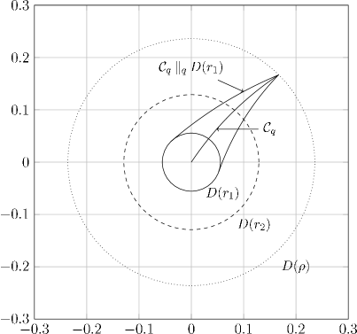
Figure 4: The boundaries of the discs and stalks when $q=-2+3i$.

We can choose the radii $\rho^{2}=r_{1}\leq r_{2}\leq\ldots\leq r_{\Lambda-1}\leq\rho$ exactly as in Section 5, and this guarantees that $D_{k}\mathbin{\|_{q}}D_{\ell}\subseteq D_{k+\ell}$.

To complete the proof of Theorem 7.1, it therefore suffices to verify the “series condition” (1) of Theorem 4.2. We shall do this, once again, by using Lemma 4.3 with $r=\rho$. Since $\rho^{2}=r_{1}\leq r_{2}\leq\cdots\leq r_{\Lambda-1}\leq\rho$, it suffices to verify that

$${\mathcal{C}}_{q}\mathbin{\|_{q}}D(r_{\Lambda-2})\;\subseteq\;D(\rho)\;.$$ (7.10)

We shall prove the stronger statement that

$${\mathcal{C}}_{q}\mathbin{\|_{q}}D(\rho)\;\subseteq\;D(\rho)\;.$$ (7.11)

Indeed, we shall prove also a strong converse to this statement, although we shall not make use of this converse.

Lemma 7.3

Let $q$ be a fixed complex number such that $|q-1|>1$, let $\rho=1/|1-q|$, and let ${\mathcal{C}}_{q}$ be defined by (7.1). Then a complex number $t$ satisfies $\{t\}\mathbin{\|_{q}}D(\rho)\subseteq D(\rho)$ if and only if $t\in{\mathcal{C}}_{q}$. [Otherwise put, we have ${\mathcal{C}}_{q}\mathbin{\|_{q}}D(\rho)\subseteq D(\rho)$, and ${\mathcal{C}}_{q}$ is the largest set with this property.]

Proof.  It is easiest to change variables once again and consider the situation in the complex $y$-plane, where parallel connection is simply multiplication $y_{e}\mathbin{\|^{Y}}y_{f}=y_{e}y_{f}$ and the curve ${\mathcal{C}}_{q}$ corresponds to the segment $[0,1]$. The relationship between $y$ and $t$ is given by the Möbius transformation

$$y\;=\;\frac{(q-1)t+1}{-t+1}\;.$$ (7.12)

Since $D(\rho)$ is a closed disc in the complex $t$-plane having the point $t_{0}=1/(1-q)$ on its boundary, the image of $D(\rho)$ in the complex $y$-plane is a closed disc $D^{Y}(\rho)$ having the origin $y_{0}=0$ on its boundary. (Here we have used $|q-1|>1$. If $|q-1|=1$, then $D^{Y}(\rho)$ is a closed half-plane having the origin on its boundary; while if $|q-1|<1$, then $D^{Y}(\rho)$ is the closed exterior of a disc having the origin on its boundary.) Now, for any closed disc $D$ having the origin on its boundary, it is easy to see that a complex number $y$ satisfies $yD\subseteq D$ if and only if $y\in[0,1]$. Back in the $t$-plane, this says that $t\in{\mathcal{C}}_{q}$.  $\Box$

Combining these results, we have:

Proof of Theorem 7.1.  We choose the radii $\rho^{2}=r_{1}\leq r_{2}\leq\ldots\leq r_{\Lambda-1}\leq\rho$ exactly as in Section 5, which guarantees that $D(r_{k})\mathbin{\|_{q}}D(r_{\ell})\subseteq D(r_{k+\ell})$. Then Lemmas 7.2, 7.3 and 4.3 guarantee that the sets $S_{k}$ defined by (7.9) satisfy the conditions (1) and (2) of Theorem 4.2. Conditions (3) and (4) of Theorem 4.2 are verified exactly as in the proof of Proposition 5.2.  $\Box$

The fact that Lemma 7.3 gives a necessary and sufficient condition suggests that there is something natural about the real antiferromagnetic regime $v_{e}\in[-1,0]$. On the other hand, our strategy of proof does not really require us to prove the strong statement (7.11); it would suffice to prove the slightly weaker statement (7.10) [or perhaps even weaker bounds], and this might allow a somewhat larger set of weights $v_{e}$. In particular, the proof of Theorem 1.2 given in [44] works naturally for the “complex antiferromagnetic regime” $|1+v_{e}|\leq 1$ (see [27] for the changes when one goes beyond this), so it is reasonable to ask whether the bounds in terms of maxmaxflow can be extended to this case, possibly with a worse constant (but still growing only linearly in $\Lambda$). We do not yet know the answer. As a warm-up, it might be helpful to study the intersection of the complex antiferromagnetic regime with the real axis, namely the “extended real antiferromagnetic regime” $v_{e}\in[-2,0]$.

8 Generalization to non-series-parallel graphs

In this section we show how our constructions can be generalized to handle graphs that are not series-parallel but are nevertheless built up by using series and parallel compositions from a fixed starting set of 2-terminal “base graphs”. We begin by stating an abstract theorem on excluding roots, which generalizes Theorems 4.1 and 4.2 to the non-series-parallel case (Section 8.1). Then we apply this result to prove Theorem 1.6 (Section 8.2).

8.1 Generalized abstract theorem on excluding roots

Here is Theorem 4.1 generalized to the non-series-parallel case:

Theorem 8.1

Let $q\neq 0$ be a fixed complex number and let $\Lambda\geq 2$ be a fixed integer. Let $S_{1}\subseteq S_{2}\subseteq\cdots\subseteq S_{\Lambda-1}$ be sets in the (finite) complex $v$-plane such that

• $S_{k}\mathbin{\bowtie^{V}_{q}}S_{\ell}\subseteq S_{\min(k,\ell)}$ for all $k,\ell$

• $S_{k}\mathbin{\|^{V}}S_{\ell}\subseteq S_{k+\ell}$ for $k+\ell\leq\Lambda-1$

Now consider any (loopless connected) 2-terminal graph $(G,s,t)$ and any nontrivial decomposition tree for $(G,s,t)$ in which all the proper constituents have between-terminals flow at most $\Lambda-1$. Suppose that we equip $G$ with edge weights $\{v_{e}\}$ such that for every leaf node $(H,a,b)$ of the decomposition tree, we have $v_{\rm eff}(H,a,b)\in S_{\lambda_{H}(a,b)}$. Then, for every node $(H,a,b)$ of the decomposition tree that has between-terminals flow $\lambda_{H}(a,b)\leq\Lambda-1$, we have $v_{\rm eff}(H,a,b)\in S_{\lambda_{H}(a,b)}$.

Now assume further that, in addition to (1) and (2), the following hypotheses hold:

• $-q\notin S_{\Lambda-1}$

• $-q\notin S_{k}\mathbin{\|^{V}}S_{\ell}$ for $k+\ell=\Lambda$

Then, for any $(G,s,t)$ and $\{v_{e}\}$ as above, such that $G$ has maxmaxflow at most $\Lambda$, we have $Z_{G}(q,{\bf v})\not=0$.

The proof of Theorem 8.1 is a minor modification of that of Theorem 4.1 and is left to the reader. There is also an obvious translation of Theorem 8.1 to the $t$-plane along the lines of Theorem 4.2, of which the statement and proof are again left to the reader.

8.2 Wheatstone bridge

The Wheatstone bridge is the 2-terminal graph ${\sf W}=(W,s,t)$ obtained from $W=K_{4}-e$ by taking the two vertices of degree $2$ to be the terminals $s$ and $t$. Note that although $K_{4}-e$ is a series-parallel graph, ${\sf W}$ is not a 2-terminal series-parallel graph (by Corollary 3.4, because $W+st=K_{4}$ is not a series-parallel graph).

Now define the class ${\mathcal{W}}$ of 2-terminal graphs to be the smallest class that contains both $K_{2}$ (with the two vertices as terminals) and ${\sf W}$ and is closed under series and parallel composition. Figure 5 shows some graphs in ${\mathcal{W}}$: the first is a 2-terminal series-parallel graph, while the second has used ${\sf W}=(W,s,t)$ in place of the “diamond” ${\sf D}=(K_{2}\mathbin{\bowtie}K_{2})\mathbin{\|}(K_{2}\mathbin{\bowtie}K_{2})$.

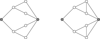
Figure 5: The graphs $(K_{2}\mathbin{\bowtie}{\sf D})\mathbin{\|}(K_{2}\mathbin{\bowtie}{\sf D})$ and $(K_{2}\mathbin{\bowtie}{\sf W})\mathbin{\|}(K_{2}\mathbin{\bowtie}{\sf W})$.

For the Wheatstone bridge, simple calculations [e.g. using (2.28)/(2.33)] show that if $v_{f}=-1$ for every edge, then the partial Tutte polynomials (2.29)/(2.30) are given by

$$A_{W,s,t}&=(q-2)(q-3)\\ B_{W,s,t}=2(q-2)$$ (8.1)

and hence

$$v_{\rm eff}(W,s,t)\;=\;\frac{2}{q-3}\;.$$ (8.2)

Expressed in terms of transmissivities, this yields

$$t_{\rm eff}(W,s,t)\;\equiv\;{v_{{\rm eff}}\over q+v_{{\rm eff}}}\;=\;\frac{2}{(q-1)(q-2)}\;.$$ (8.3)

The maximum flow between the terminals of the Wheatstone bridge is equal to $2$. Therefore, as far as the chromatic roots of graphs in ${\mathcal{W}}$ are concerned, the Wheatstone bridge just behaves as a sort of “super-edge” with capacity (in the flow-carrying sense) equal to 2 and effective transmissivity given by (8.3): that is the upshot of Theorem 8.1.

Now suppose that $S_{1}\subseteq S_{2}\subseteq\cdots\subseteq S_{\Lambda-1}$ is a set of regions in the complex $t$-plane certifying (via Theorem 4.2) that a particular value of $q$ is not the chromatic root of any series-parallel graph of maxmaxflow at most $\Lambda$. Then, by Theorem 8.1, the same set of regions will suffice for graphs in ${\mathcal{W}}$ of maxmaxflow at most $\Lambda$, provided only that $2/[(q-1)(q-2)]\in S_{2}$.

So, under the same hypothesis $|q-1|\geq 1/\rho^{\star}_{\Lambda}$ as in Theorem 5.1, let us again choose “point+disk” regions (5.6) with radii $r_{k}$ given by (5.40). We then have

$$r_{2}\;=\;\rho\,{X^{2}-1\over 1-\rho X^{2}}\qquad\hbox{where}\quad\rho\,=\,{1\over|q-1|}\;\;\hbox{and}\;\;X\,=\,\biggl{(}{2\over 1+\rho}\biggr{)}^{1/(\Lambda-1)}\;.$$ (8.4)

Therefore, these regions suffice to show that $q$ is not a chromatic root of any graph in ${\mathcal{W}}$ whenever we have

$$\frac{2}{|q-2|}\;\leq\;{X^{2}-1\over 1-\rho X^{2}}$$ (8.5)

in addition to the hypothesis $|q-1|\geq 1/\rho^{\star}_{\Lambda}$. We have therefore proven:

Theorem 8.2

Fix an integer $\Lambda\geq 3$, and let ${\sf G}=(G,s,t)$ be a 2-terminal graph in the class ${\mathcal{W}}$ such that $G$ has maxmaxflow at most $\Lambda$. Then the chromatic polynomial $P_{G}(q)$ is nonvanishing whenever

$$|q-1|\>\geq\>1/\rho^{\star}_{\Lambda}\quad\hbox{and}\quad|q-2|\>\geq\>{2(1-\rho X^{2})\over X^{2}-1}\;,$$ (8.6)

where $\rho_{\Lambda}^{\star}$ is defined by (5.1) and $\rho$ and $X$ are defined by (8.4).

When $\Lambda=3$, the condition (8.5) becomes particularly simple as it reduces to

$$|q-2|\;\geq\;2\;.$$ (8.7)

The disk $|q-2|<2$ extends only slightly beyond the disk $|q-1|<1/\rho_{3}^{\star}$, with the greatest protrusion $4-(1+1/\rho_{3}^{\star})\approx 0.34103\ldots$ occurring on the positive real axis. Thus, the region guaranteed to contain the chromatic roots of the graphs in ${\mathcal{W}}$ of maxmaxflow 3, given by the union of the discs $|q-1|<1/\rho_{3}^{\star}$ and $|q-2|<2$ (the left-hand picture of Figure 6), is only slightly larger than the region $|q-1|<1/\rho_{3}^{\star}$ guaranteed to contain the chromatic roots of series-parallel graphs of maxmaxflow 3.

For $\Lambda>3$, the right-hand side of (8.5) is not independent of $\rho$, and so the corresponding region is not quite a circular disk (as it depends on the phase of $q$), but rather a slightly squashed disk. Nevertheless, the corresponding region always extends slightly past the region $|q-1|<1/\rho_{\Lambda}^{\star}$, with maximum protrusion again on the positive real axis (see the right-hand picture of Figure 6 for $\Lambda=4$).

In order to obtain a simple sufficient condition depending only on $|q-1|$, we can use the trivial bound $|q-2|\geq|q-1|-1=\rho^{-1}-1$. After some simple algebra we find that a sufficient condition on $\rho$ for (8.5) to be satisfied is that

$$\left(\frac{2}{1+\rho}\right)^{2/{(\Lambda-1)}}\;\geq\;\frac{1+\rho}{1-\rho+2\rho^{2}}\;,$$ (8.8)

or equivalently that

$$(1+\rho)^{\Lambda+1}\;\leq\;4(1-\rho+2\rho^{2})^{\Lambda-1}\;.$$ (8.9)

This condition is handled by the following analogue of Lemma 5.6:

Lemma 8.3

For $\rho\in(0,1)$ and real $\Lambda>2$, the following are equivalent:

• $(1+\rho)^{\Lambda+1}\>\leq\>4(1-\rho+2\rho^{2})^{\Lambda-1}$.

• $\rho\leq\rho^{\star\star}_{\Lambda}$, where $\rho^{\star\star}_{\Lambda}$ is the unique solution of

  $$(1+\rho)^{\Lambda+1}\;=\;4(1-\rho+2\rho^{2})^{\Lambda-1}$$ (8.10)

  in the interval $(0,1)$.

Deferring temporarily the proof of this Lemma, let us observe that from (5.1) it follows easily that

$$\left(\frac{2}{1+\rho_{\Lambda}^{\star}}\right)^{1/{(\Lambda-1)}}\;=\;\frac{1+\rho_{\Lambda}^{\star}}{1+{\rho_{\Lambda}^{\star}}^{2}}\;<\;\frac{1+\rho_{\Lambda}^{\star}}{1-\rho_{\Lambda}^{\star}+2{\rho_{\Lambda}^{\star}}^{2}}\;,$$ (8.11)

so that the condition (8.8) is false when $\rho=\rho_{\Lambda}^{\star}$, or in other words we have $\rho_{\Lambda}^{\star\star}<\rho_{\Lambda}^{\star}$ whenever $\Lambda>2$ (see Table 1). We have therefore proven (subject to the proof of Lemma 8.3):

Corollary 8.4

Fix an integer $\Lambda\geq 3$, and let ${\sf G}=(G,s,t)$ be a 2-terminal graph in the class ${\mathcal{W}}$ such that $G$ has maxmaxflow at most $\Lambda$. Then the chromatic polynomial $P_{G}(q)$ is nonvanishing whenever

$$|q-1|\;\geq\;1/\rho^{\star\star}_{\Lambda}\;,$$ (8.12)

where $\rho_{\Lambda}^{\star\star}$ is the unique solution of

$$(1+\rho)^{\Lambda+1}\;=\;4(1-\rho+2\rho^{2})^{\Lambda-1}$$ (8.13)

in the interval $(0,1)$.

Since the bound $|q-2|\geq|q-1|-1$ holds as equality when $q$ is real and $q>2$, we see that the condition (8.8) is also necessary for (8.5) when $q$ is real and positive; or in other words, the circle $|q-1|=1/\rho_{\Lambda}^{\star\star}$ coincides with the boundary of the region (8.5) on the positive real axis, but lies outside of it elsewhere. Figure 6 shows how these regions compare for $\Lambda=3,4$.

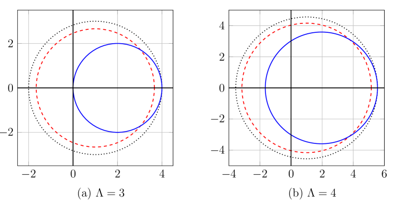
Figure 6: Circles $|q-1|=1/\rho_{\Lambda}^{*}$ (red dashed) and $|q-1|=1/\rho_{\Lambda}^{**}$ (black dotted) and the boundary of the region (8.5) [blue solid curve], for (a) $\Lambda=3$ and (b) $\Lambda=4$.

$\Lambda$	$\rho^{\star}_{\Lambda}$	$\rho^{\star\star}_{\Lambda}$	$1/\rho^{\star}_{\Lambda}$	$1/\rho^{\star\star}_{\Lambda}$
2	1	1.000000	1	1.000000
3	0.376086	0.333333	2.658967	3.000000
4	0.240380	0.219471	4.160076	4.556417
5	0.177591	0.165204	5.630929	6.053134
6	0.141038	0.132841	7.090297	7.527812
7	0.117041	0.111213	8.544040	8.991750
8	0.100054	0.095697	9.994599	10.449611
9	0.087388	0.084008	11.443181	11.903688
10	0.077577	0.074877	12.890449	13.355246

Table 1: Values of $\rho^{\star}_{\Lambda}$, $\rho^{\star\star}_{\Lambda}$, $1/\rho^{\star}_{\Lambda}$, $1/\rho^{\star\star}_{\Lambda}$ for $2\leq\Lambda\leq 10$.

Proof of Lemma 8.3.  Consider the function

$$f_{\Lambda}(\rho)\;=\;(\Lambda+1)\log(1+\rho)\,-\,(\Lambda-1)\log(1-\rho+2\rho^{2})\;.$$ (8.14)

Its first two derivatives are

$$f^{\prime}_{\Lambda}(\rho)&={\Lambda+1\over 1+\rho}\,-\,{(\Lambda-1)(4\rho-1)\over 1-\rho+2\rho^{2}}\\ f^{\prime\prime}_{\Lambda}(\rho)=-\,{(6+4\rho+18\rho^{2}-24\rho^{3}+4\rho^{4})\,+\,(\Lambda-2)(4+8\rho+8\rho^{2}-16\rho^{3}-4\rho^{4})\over(1+\rho)^{2}(1-\rho+2\rho^{2})^{2}}\\$$ (8.15)

For $0\leq\rho\leq 1$ we manifestly have $6+4\rho+18\rho^{2}-24\rho^{3}+4\rho^{4}\geq 4\rho-4\rho^{3}\geq 0$ and $4+8\rho+8\rho^{2}-16\rho^{3}-4\rho^{4}\geq 4-4\rho^{4}\geq 0$, with strict inequality when $0<\rho<1$; hence $f_{\Lambda}$ is strictly concave on $[0,1]$ whenever $\Lambda\geq 2$. We have $f_{\Lambda}(0)=0$, $f^{\prime}_{\Lambda}(0)=2\Lambda>0$, $f_{\Lambda}(1)=\log 4$ and $f^{\prime}_{\Lambda}(1)=-(\Lambda-2)$. Therefore, for $\Lambda>2$, there is a unique $\rho^{\star\star}_{\Lambda}\in(0,1)$ satisfying $f_{\Lambda}(\rho^{\star\star}_{\Lambda})=\log 4$; and for $\rho\in[0,1)$ we have $f_{\Lambda}(\rho)\leq\log 4$ if and only if $\rho\leq\rho^{\star\star}_{\Lambda}$. This proves the equivalence of (a) and (b) for all real $\Lambda>2$.  $\Box$

Finally, let us deduce Theorem 1.6 as an immediate consequence of Corollary 8.4, by proving that $\rho^{\star\star}_{\Lambda}>(\log 2)/(\Lambda-\log 2)$ for all integers $\Lambda\geq 3$, or equivalently (in view of Lemma 8.3) that $(1+\rho)^{\Lambda+1}<4(1-\rho+2\rho^{2})^{\Lambda-1}$ when $\rho=(\log 2)/(\Lambda-\log 2)$. We shall actually prove this for all real $\Lambda>2\log 2\approx 1.386294$. Taking logarithms and parametrizing by $\rho\in(0,1)$, we see that this is equivalent to the following claim:

Lemma 8.5

The function

$$g(\rho)&=\rho\left[2\log 2\>+\>\biggl{(}{\log 2\over\rho}\,+\,\log 2\,-\,1\biggr{)}\,\log(1-\rho+2\rho^{2})\>-\>\biggl{(}{\log 2\over\rho}+\log 2+1\biggr{)}\,\log(1+\rho)\right]\\ \\ =2\rho\log\biggl{(}{2\over 1+\rho}\biggr{)}\,-\,(\log 2)\log\biggl{(}{1+\rho\over 1-\rho+2\rho^{2}}\biggr{)}-(\log 2-1)\rho\log\biggl{(}{1+\rho\over 1-\rho+2\rho^{2}}\biggr{)}$$ (8.16)

is strictly positive for $0<\rho<1$.

Proof.  The second derivative of $g$ is given by $g^{\prime\prime}(\rho)=h(\rho)\times\rho/(1+\rho^{2}+2\rho^{3})^{2}$ where

$$h(\rho)\;=\;-(12-4\log 2)\rho^{4}\,-\,12\rho^{3}\,-\,(2+8\log 2)\rho^{2}\,-\,(24-16\log 2)\rho\,+\,(20\log 2-6)\;.$$ (8.17)

All the coefficients of $h(\rho)$ are strictly negative except for the last (constant) term, so we have $h^{\prime}(\rho)<0$ for all $\rho\geq 0$. Since $h(0)=20\log 2-6>0$ and $h(1)=32\log 2-56<0$ and $h$ is strictly decreasing for $\rho\geq 0$, it follows that $h(\rho)$ has exactly one positive real root $\rho^{*}$ and that it lies between 0 and 1 (by computer $\rho^{*}\approx 0.417655$). Therefore $g$ is strictly convex on $[0,\rho^{*}]$ and strictly concave on $[\rho^{*},\infty)$. Since $g(0)=g^{\prime}(0)=0$, we have $g(\rho)>0$ for $\rho\in(0,\rho^{*}]$. Moreover, since $g(\rho^{*})>0$ and $g(1)=0$ and $g$ is strictly concave on $[\rho^{*},1]$, we have $g(\rho)>0$ for $\rho\in[\rho^{*},1)$. Hence $g(\rho)>0$ for all $\rho\in(0,1)$, as claimed.  $\Box$

Remark. A straightforward calculation shows that the large-$\Lambda$ asymptotic behavior of $\rho^{\star\star}_{\Lambda}$ is given by

$$\rho^{\star\star}_{\Lambda}\;=\;(\log 2)\Biggl{[}{1\over\Lambda-1}\,+\,{\log 2-1\over(\Lambda-1)^{2}}\,+\,{16\log^{2}2-15\log 2+6\over 6(\Lambda-1)^{3}}\,+\,\ldots\Biggr{]}$$ (8.18)

and hence

$${1\over\rho^{\star\star}_{\Lambda}}\;=\;{\Lambda-1\over\log 2}\,-\,{\log 2-1\over\log 2}\,-\,{10\log 2-3\over 6(\Lambda-1)}\,+\,\ldots\;\;.$$ (8.19)

So the inequality $\rho^{\star\star}_{\Lambda}>(\log 2)/(\Lambda-\log 2)$ captures the first two terms of the large-$\Lambda$ asymptotic behavior.  $\Box$

Appendix A Parallel and series connection on the Riemann sphere

In this appendix we shall define parallel and series connection for edge weights $\{v_{e}\}$ (or $\{y_{e}\}$ or $\{t_{e}\}$) lying in the Riemann sphere ${\overline{\mathbb{C}}}={\mathbb{C}}\cup\{\infty\}$; in our opinion this is the most natural way to view these maps. We shall always treat ${\overline{\mathbb{C}}}$ as a one-dimensional complex manifold equipped with its usual holomorphic structure.

We begin with some general remarks concerning rational functions of several complex variables.

At an algebraic level, there is no difficulty in defining the field ${\mathbb{K}}(z_{1},\ldots,z_{n})$ of rational functions in an arbitrary number of indeterminates $z_{1},\ldots,z_{n}$ over an arbitrary field ${\mathbb{K}}$. The elements of this field are simply equivalence classes of ratios $P/Q$ where $P,Q\in{\mathbb{K}}[z_{1},\ldots,z_{n}]$ are polynomials with $Q\not\equiv 0$, and the field operations are defined in the obvious way.

However, when ${\mathbb{K}}={\mathbb{C}}$ and we wish to consider rational functions from an analytic point of view, there is a fundamental difference between the cases $n=1$ and $n>1$. This is a consequence of the following theorem [39, Theorem 1.3.2]: Let $P,Q$ be relatively prime polynomials in $n$ complex variables, and let $z_{0}\in{\mathbb{C}}^{n}$ be such that $P(z_{0})=Q(z_{0})=0$. (Of course, this can happen only when $n>1$.) Then in every neighborhood $U\ni z_{0}$, the function $P/Q$ takes unambiguously all possible values in ${\overline{\mathbb{C}}}$ (in addition to also taking the undefined value $0/0$). Therefore, if the zero sets ${\mathcal{Z}}(P)$ and ${\mathcal{Z}}(Q)$ have a nonempty intersection, the rational function $P/Q$ cannot even be defined as a continuous function (much less a holomorphic one) in a neighborhood of the intersection point. On the other hand, if we cut out the “bad points” ${\mathcal{Z}}(P)\cap{\mathcal{Z}}(Q)$, then $P/Q$ is a well-defined holomorphic function from ${\mathbb{C}}^{n}\setminus({\mathcal{Z}}(P)\cap{\mathcal{Z}}(Q))$ into ${\overline{\mathbb{C}}}$. And with a little more work we can also allow $\infty$ as a possible value for $z_{1},\ldots,z_{n}$ (expanding the “bad set” as needed).

In our case we want to make sense of the parallel and series maps (in $n=2$ variables) defined in (2.14)–(2.19). Note first that the maps (2.12)/(2.13) between the $v$-, $t$- and $y$-variables are invertible Möbius transformations, hence biholomorphic maps of the Riemann sphere ${\overline{\mathbb{C}}}$ onto itself, whenever $q\neq 0,\infty$ (as we shall assume henceforth). We can therefore define the parallel connection $\mathbin{\|}$ as follows: Map first into the $y$ variables; use the definition $y_{e}\mathbin{\|}^{Y}y_{f}=y_{e}y_{f}$; then map back. Now, the operation of multiplication, $(y_{1},y_{2})\mapsto y_{1}y_{2}$, is unambiguously defined for $y_{1}$ and $y_{2}$ in the Riemann sphere, with two exceptions: $0\cdot\infty$ and $\infty\cdot 0$ are ill-defined. Deleting these two “bad points”, we see that multiplication is a well-defined holomorphic map from ${\overline{\mathbb{C}}}^{2}\setminus\{(0,\infty),\,(\infty,0)\}$ into ${\overline{\mathbb{C}}}$. It follows that

• the parallel connection $\mathbin{\|}^{Y}$ is well-defined for $(y_{e},y_{f})\in{\overline{\mathbb{C}}}^{2}\setminus\{(0,\infty),\,(\infty,0)\}$,

• the parallel connection $\mathbin{\|}^{V}$ is well-defined for $(v_{e},v_{f})\in{\overline{\mathbb{C}}}^{2}\setminus\{(-1,\infty),\,(\infty,-1)\}$, and

• the parallel connection $\mathbin{\|^{T}_{q}}$ is well-defined for $(t_{e},t_{f})\in{\overline{\mathbb{C}}}^{2}\setminus\{(1/(1-q),1),\,(1,1/(1-q))\}$.

Only at the two “bad points” do we declare that the parallel connection takes the value “undefined”.

Likewise, we can define the series connection $\mathbin{\bowtie}$ as follows: Map first into the $t$ variables; use the definition $t_{e}\mathbin{\bowtie}^{Y}t_{f}=t_{e}t_{f}$; then map back. It follows that

• the series connection $\mathbin{\bowtie}^{T}$ is well-defined for $(t_{e},t_{f})\in{\overline{\mathbb{C}}}^{2}\setminus\{(0,\infty),\,(\infty,0)\}$,

• the series connection $\mathbin{\bowtie^{V}_{q}}$ is well-defined for $(v_{e},v_{f})\in{\overline{\mathbb{C}}}^{2}\setminus\{(0,-q),\,(-q,0)\}$, and

• the series connection $\mathbin{\bowtie^{Y}_{q}}$ is well-defined for $(y_{e},y_{f})\in{\overline{\mathbb{C}}}^{2}\setminus\{(1,1-q),\,(1-q,1)\}$.

At the two “bad points” we assign once again the value “undefined”.

Finally, we declare that if one or both of the inputs to a $\mathbin{\|}^{\sharp}$ or $\mathbin{\bowtie}^{\sharp}$ operation ($\sharp=V$, $T$ or $Y$) is “undefined”, then the output is also “undefined”. The operations $\mathbin{\|}^{\sharp}$ and $\mathbin{\bowtie}^{\sharp}$ then become well-defined maps ${\widetilde{\mathbb{C}}}\times{\widetilde{\mathbb{C}}}\to{\widetilde{\mathbb{C}}}$, where ${\widetilde{\mathbb{C}}}={\overline{\mathbb{C}}}\cup\{\hbox{undefined}\}={\mathbb{C}}\cup\{\infty,\hbox{undefined}\}$, and moreover these operations for different $\sharp$ intertwine correctly with the Möbius transformations that map one set of variables ($v$, $t$ or $y$) to another.

Appendix B Chromatic roots of leaf-joined trees

For integers $r\geq 2$ and $n\geq 1$, the leaf-joined tree of branching factor $r$ and depth $n$ is defined to be the graph $G_{n}^{r}$ obtained by taking a complete $r$-ary rooted tree of height $n$ and then identifying all the leaves into a single vertex. Our goal in this appendix is to study, for fixed $r$, the accumulation points as $n\to\infty$ of the chromatic roots of the family $\{G_{n}^{r}\}_{n\geq 1}$. In particular, we shall prove the following:

Theorem B.1 (= Theorem 3.11)

For fixed $r\geq 2$, every point of the circle $|q-1|=r$ is a limit point of chromatic roots for the family $\{G_{n}^{r}\}_{n\geq 1}$ of leaf-joined trees of branching factor $r$. [More precisely, for every $q_{0}$ satisfying $|q_{0}-1|=r$ and every $\epsilon>0$, there exists $n_{0}=n_{0}(q_{0},\epsilon)$ such that for all $n\geq n_{0}$ the graph $G_{n}^{r}$ has a chromatic root $q$ lying in the disc $|q-q_{0}|<\epsilon$.]

To lighten the notation, we shall henceforth fix $r\geq 2$ and write $G_{n}$ in place of $G_{n}^{r}$. We shall regard $G_{n}$ as a 2-terminal graph in which the terminals are the root and the identified-leaves vertex. It is easy to see that $G_{n}$ is in fact 2-terminal series-parallel, as it can be defined recursively as follows:

$$G_{1}&=K_{2}^{(r)}\\ G_{n+1}=(K_{2}\mathbin{\bowtie}G_{n})^{\mathbin{\|}r}{}$$ (B.1)

where $K_{2}^{(r)}$ is the graph with two vertices connected by $r$ parallel edges, and $G^{\mathbin{\|}r}$ denotes the parallel connection of $r$ copies of $G$.

To every edge of $G_{n}$ we assign the same weight $v_{\sharp}$ and we study the (bivariate) Tutte polynomial $Z_{G_{n}}(q,v_{\sharp})$. In particular, by taking $v_{\sharp}=-1$ we can study the chromatic polynomial $P_{G_{n}}(q)$. We shall prove Theorem B.1 by tracking the evolution of the “effective coupling” $v_{\rm eff}(G_{n})$ according to (LABEL:eq.app_tree.def_Gn.b). In doing this we shall adopt the approach set forth in Appendix A, where $v_{\rm eff}$ is considered to lie in the Riemann sphere ${\overline{\mathbb{C}}}={\mathbb{C}}\cup\{\infty\}$. Please note that the parallel and series connections arising in (LABEL:eq.app_tree.def_Gn.b) are always well-defined in the sense of Appendix A: the series connections avoid the “bad points” $(v_{1},v_{2})=(0,-q)$ and $(-q,0)$ because we always have $v_{1}=v_{\sharp}$ (corresponding to the graph $K_{2}$) and we shall assume that $q\notin\{0,-v_{\sharp}\}$; while the parallel connections avoid the “bad points” $(v_{1},v_{2})=(-1,\infty)$ and $(\infty,-1)$ because we perform repeated parallel connections of the same graph $K_{2}\mathbin{\bowtie}G_{n}$ and hence at every stage $v_{1}$ and $v_{2}$ are either both finite or both infinite.

The basic idea is now that $Z_{G_{n}}(q,v_{\sharp})$ equals $q[q+v_{\rm eff}(G_{n})]$ times some prefactors; so if we temporarily put aside the problem of the prefactors, we can conclude that $Z_{G_{n}}(q,v_{\sharp})=0$ if and only if $v_{\rm eff}(G_{n})=-q$ (provided that $q\neq 0$, as we shall assume henceforth). To be more precise (and to handle the problem of the prefactors), let us use Proposition 2.4 to compute the polynomials $A_{n}(q,v_{\sharp})\equiv A_{G_{n},s,t}$ and $B_{n}(q,v_{\sharp})\equiv B_{G_{n},s,t}$ that were defined in (2.29)/(2.30); from these we can obtain $Z_{G_{n}}(q,v_{\sharp})=q^{2}A_{n}(q,v_{\sharp})+qB_{n}(q,v_{\sharp})$. Defining the intermediate graphs $G^{\prime}_{n}=K_{2}\mathbin{\bowtie}G_{n}$ and the corresponding quantities $A^{\prime}_{n}\equiv A_{G^{\prime}_{n},s,t}$ and $B^{\prime}_{n}\equiv B_{G^{\prime}_{n},s,t}$, we have from Proposition 2.4(b)

$$A^{\prime}_{n}&=(q+v_{\sharp})A_{n}+B_{n}\\ B^{\prime}_{n}=v_{\sharp}B_{n}$$ (B.2)

and thence from Proposition 2.4(a)

$$A_{n+1}&=(A^{\prime}_{n})^{r}\\ =[(q+v_{\sharp})A_{n}+B_{n}]^{r}\\ B_{n+1}=(A^{\prime}_{n}+B^{\prime}_{n})^{r}\,-\,(A^{\prime}_{n})^{r}\\ =[(q+v_{\sharp})A_{n}+(1+v_{\sharp})B_{n}]^{r}\,-\,[(q+v_{\sharp})A_{n}+B_{n}]^{r}$$ (B.3)

The initial condition for this recursion is

$$A_{1}\>=\>1,\qquad B_{1}\>=\>(1+v_{\sharp})^{r}\,-\,1$$ (B.4)

or equivalently

$$A_{0}\>=\>0,\qquad B_{0}\>=\>1\;.$$ (B.5)

Note now that the polynomials $A_{n}$ and $B_{n}$ have no common zeros in ${\mathbb{C}}^{2}\setminus\{(q,v_{\sharp})\colon\>q+v_{\sharp}=0\}$: this follows by induction from (B.3), since $A_{n+1}=B_{n+1}=0$ and $q+v_{\sharp}\neq 0$ imply $A_{n}=B_{n}=0$. [This observation is just a rephrasing of the previously-observed fact that the series and parallel connections are here well-defined whenever $q\notin\{0,-v_{\sharp}\}$.] Therefore, provided that $q\notin\{0,-v_{\sharp}\}$, we have $Z_{G_{n}}(q,v_{\sharp})=0$ if and only if $A_{n}(q,v_{\sharp})\neq 0$ and $B_{n}(q,v_{\sharp})/A_{n}(q,v_{\sharp})=-q$.

But $B_{n}/A_{n}$ is precisely what we have called $v_{\rm eff}(G_{n})$ [cf. (2.31)]. Writing $v_{n}=v_{\rm eff}(G_{n})$ to lighten the notation, we obtain from (B.3) [or equivalently from (2.40)/(2.44)] the recursion

$$v_{n+1}\;=\;(v_{\sharp}\,\mathbin{\bowtie^{V}_{q}}v_{n})^{\mathbin{\|}^{V}r}\;=\;\left(1\,+\,{v_{\sharp}v_{n}\over q+v_{\sharp}+v_{n}}\right)^{\!r}\>-\>1$$ (B.6)

with initial condition

$$v_{1}\;=\;(1+v_{\sharp})^{r}\,-\,1$$ (B.7)

or

$$v_{0}\;=\;\infty\;.$$ (B.8)

And provided that $q\notin\{0,-v_{\sharp}\}$, we have proven that $Z_{G_{n}}(q,v_{\sharp})=0$ if and only if $v_{n}=-q$.

Since the final operation in (LABEL:eq.app_tree.def_Gn.b) is parallel composition, it is actually more convenient to use the $y$-variables, i.e. $y_{\sharp}=1+v_{\sharp}$ and $y_{n}=y_{\rm eff}(G_{n})=1+v_{\rm eff}(G_{n})$. We then have

$$y_{0}&=\infty\\ y_{1}=y_{\sharp}^{r}\\ y_{n+1}=(y_{\sharp}\,\mathbin{\bowtie}_{q}^{Y}y_{n})^{\mathbin{\|}^{Y}r}\;=\;\left({q-1+y_{\sharp}y_{n}\over q-2+y_{\sharp}+y_{n}}\right)^{\!r}$$ (B.9)

or in other words $y_{n+1}=R_{q}(y_{n})$ where

$$R_{q}(y)\;=\;\left({q-1+y_{\sharp}y\over q-2+y_{\sharp}+y}\right)^{\!r}\;.$$ (B.10)

We have $Z_{G_{n}}(q,v_{\sharp})=0$ if and only if $y_{n}=1-q$. We summarize the foregoing discussion as follows:

Lemma B.2

For $v_{\sharp}\in{\mathbb{C}}$, $q\in{\mathbb{C}}\setminus\{0,-v_{\sharp}\}$ and $n\geq 1$, we have

$$Z_{G_{n}}(q,v_{\sharp})\,=\,0\quad\text{if and only if}\quad R_{q}^{n}(\infty)\,=\,1-q\;,$$

where $R_{q}$ is the map (B.10) with $y_{\sharp}=1+v_{\sharp}$.

We are thus interested in the iteration of the rational function $R_{q}$, considered as a map from the Riemann sphere ${\overline{\mathbb{C}}}={\mathbb{C}}\cup\{\infty\}$ to itself, and so we are naturally led to the theory of holomorphic dynamics [3, 19, 48, 33].

In what follows we shall restrict attention to the chromatic-polynomial case $y_{\sharp}=0$, which turns out to behave in a simpler way than $y_{\sharp}\neq 0$. We must therefore study the iteration of the map

$$R_{q}(y)\;=\;\left({q-1\over q-2+y}\right)^{\!r}$$ (B.11)

with initial condition

$$y_{0}&=\infty\\ y_{1}=0$$ (B.12)

Provided that $q\neq 1$ (which is simply our assumption $q\neq-v_{\sharp}$ specialized to the chromatic-polynomial case $v_{\sharp}=-1$), the map $R_{q}$ is a rational function of degree $r$.

We now proceed to analyze the properties of the map $R_{q}$ defined by (B.11). Elementary calculus proves the following two lemmas:

Lemma B.3

Fix $y_{\sharp}=0$ and $q\neq 1$. Then the critical points of the map $R_{q}$ are $2-q$ and $\infty$, each of multiplicity $r-1$. Moreover, there is only one critical orbit, because one critical point maps onto the other:

$$2-q\;\mapsto\;\infty\;\mapsto\;0\;\mapsto\;\left({q-1\over q-2}\right)^{\!r}\;\mapsto\;\ldots\;.$$ (B.13)

The fact that there is only one critical orbit is what makes the case $y_{\sharp}=0$ simpler than $y_{\sharp}\neq 0$.

Lemma B.4

Fix $y_{\sharp}=0$ and $q\neq 1$. Then the map $R_{q}$ has a fixed point at $y=1$, with multiplier $\lambda=-r/(q-1)$. In particular, this fixed point is attractive (but not superattractive) if $|q-1|>r$, marginal if $|q-1|=r$, and repulsive if $|q-1|<r$.

From Lemmas B.3 and B.4 we can infer the following:

Corollary B.5

Fix $y_{\sharp}=0$ and $|q-1|>r$. Then:

• The initial condition $y_{0}=\infty$ is attracted to the attractive fixed point at $y=1$, but without falling onto it: that is, $\lim\limits_{n\to\infty}R_{q}^{n}(\infty)=1$ but $R_{q}^{n}(\infty)\neq 1$ for all $n\geq 0$.

• The map $R_{q}$ has no attractive or parabolic cycles other than the attractive fixed point at $y=1$.

Proof.  It is known [3, Theorems 9.3.1 and 9.3.2] that every attractive or parabolic cycle contains a critical point within its immediate basin of attraction, and that this critical point has an infinite forward orbit that lies entirely within the immediate basin of attraction and converges to the cycle without falling onto it. Since in the present case there are only two critical points ($2-q$ and $\infty$) and only one critical orbit ($2-q\mapsto\infty\mapsto\ldots$), it follows that $\infty$ and its iterates (that is, the entire critical orbit except perhaps $2-q$) lie within the immediate basin of attraction of the attractive fixed point at $y=1$ and converge to it without falling onto it. It also follows that there cannot exist any other attractive or parabolic cycles.  $\Box$

Part (a) of Corollary B.5 will play a central role in our argument. Part (b) is very interesting to know, but we will not need to use it.

Let us now recall [3, Definition 4.1.1 and Theorem 4.1.4] that a point $z$ is called exceptional for a rational map $R$ if its backward orbit is finite; we denote by $E(R)$ the set of all the exceptional points. The following characterization is well known:

Proposition B.6

[3, Theorems 4.1.2 and 4.1.4]   A rational map $R$ of degree $d\geq 2$ has at most two exceptional points. Exactly one of the following possibilities holds:

• $E(R)=\varnothing$.

• $E(R)=\{z\}$, and $z$ is a superattractive fixed point satisfying $R^{-1}(\{z\})=\{z\}$. In this case $R$ is conjugate to a polynomial of degree $d$.

• $E(R)=\{z_{1},z_{2}\}$, and $z_{1},z_{2}$ are superattractive fixed points satisfying $R^{-1}(\{z_{i}\})=\{z_{i}\}$ $[i=1,2]$. In this case $R$ is conjugate to the map $z\mapsto z^{d}$.

• $E(R)=\{z_{1},z_{2}\}$, and $\{z_{1},z_{2}\}$ form a superattractive cycle of period 2 satisfying $R^{-1}(\{z_{1}\})=\{z_{2}\}$ and $R^{-1}(\{z_{2}\})=\{z_{1}\}$. In this case $R$ is conjugate to the map $z\mapsto z^{-d}$.

In particular, an exceptional point is always a critical point and a critical value.

Using this characterization of exceptional points, we can determine the exceptional set for our maps $R_{q}$ as an immediate consequence of Lemma B.3:

Lemma B.7

Fix $y_{\sharp}=0$ and $q\neq 1$. Then

$$E(R_{q})\;=\;\begin{cases}\{0,\infty\}&\text{\rm if $q=2$}\\[2.84526pt] \varnothing&\text{\rm if $q\neq 2$}\end{cases}$$ (B.14)

In our case we are dealing, not with a single rational map $R$, but with a family of rational maps $\{R_{q}\}_{q\in{\mathbb{C}}\setminus\{1\}}$ that depend analytically (= holomorphically) on the complex parameter $q$. So let us recall some of the general theory [30, 1] concerning the iteration of holomorphic families of rational maps.

The basic setup is as follows: We are given a family $\{R_{\lambda}\}_{\lambda\in\Lambda}$ of rational maps (of degree $d\geq 2$) parametrized holomorphically by $\lambda\in\Lambda$, where $\Lambda$ is a connected finite-dimensional complex manifold. We are also given a holomorphically varying initial point $Z_{\lambda}\in{\overline{\mathbb{C}}}$. Our goal is to understand the joint dynamics of the pair $(R_{\lambda},Z_{\lambda})$, i.e. the behavior of the family of maps $\lambda\mapsto R_{\lambda}^{n}(Z_{\lambda})$ ($n\geq 0$). We say that a point $\lambda_{0}\in\Lambda$ is a regular point for the pair $(R_{\lambda},Z_{\lambda})$ if the family $\{R_{\lambda}^{n}(Z_{\lambda})\}$ is normal in some neighborhood of $\lambda_{0}$, and an irregular point otherwise. We denote by ${\mathfrak{R}}$ (resp. ${\mathfrak{I}}$) the set of regular (resp. irregular) points; these sets are open and closed, respectively. A domain of regularity for the pair $(R_{\lambda},Z_{\lambda})$ is a connected open subset of ${\mathfrak{R}}$.

One rather trivial way for the family $\{R_{\lambda}^{n}(Z_{\lambda})\}$ to be normal is for it to reduce to a finite set of maps. This case corresponds to $Z_{\lambda}$ being persistently preperiodic, i.e. there exist $m>n\geq 0$ such that $R_{\lambda}^{m}(Z_{\lambda})=R_{\lambda}^{n}(Z_{\lambda})$ for all $\lambda\in\Lambda$. The papers [30, 1] studied the regular and irregular sets for the pair $(R_{\lambda},Z_{\lambda})$ under the assumption that $Z_{\lambda}$ is not persistently preperiodic. One of the simpler results from these papers — which will be our main tool in what follows — is the following:

Proposition B.8

[30, Proposition 3.1] [1, Proposition 4.1]   Let $\lambda_{0}\in\Lambda$ and $z_{0}\in{\overline{\mathbb{C}}}$ be such that $\lim_{n\to\infty}R^{np}_{\lambda_{0}}(z_{0})=\zeta_{\lambda_{0}}$, where $\zeta_{\lambda_{0}}$ is an attractive periodic point of period $p$ for $R_{\lambda_{0}}$. Then:

• There exist open sets $V\ni\lambda_{0}$ and $W\ni z_{0}$ and a holomorphic function $\zeta_{\lambda}$ defined for $\lambda\in V$ and taking the given value at $\lambda_{0}$, such that $\zeta_{\lambda}$ is an attractive periodic point of period $p$ for $R_{\lambda}$ for all $\lambda\in V$, and $\lim_{n\to\infty}R^{np}_{\lambda}(z)=\zeta_{\lambda}$ uniformly on compact subsets of $V\times W$.

• $\lambda_{0}$ is a regular point for every pair $(R_{\lambda},Z_{\lambda})$ satisfying $Z_{\lambda_{0}}=z_{0}$.

• Suppose that $Z_{\lambda}$ is a holomorphic path satisfying $Z_{\lambda_{0}}=z_{0}$, and that $U\ni\lambda_{0}$ is a domain of regularity for $(R_{\lambda},Z_{\lambda})$. Then $\lim_{n\to\infty}R^{np}_{\lambda}(Z_{\lambda})\equiv\zeta_{\lambda}$ exists for all $\lambda\in U$ [uniformly on compact subsets of $U$] and satisfies $R_{\lambda}^{p}(\zeta_{\lambda})=\zeta_{\lambda}$. Moreover, if $Z_{\lambda}$ is not persistently preperiodic, then $\zeta_{\lambda}$ remains attractive [i.e. satisfies $|(DR_{\lambda}^{p})(\zeta_{\lambda})|<1$] and of period $p$, for all $\lambda\in U$.

Let us now apply Proposition B.8 to our family $R_{\lambda}=R_{q}$ with initial condition $Z_{\lambda}=\infty$. We first need the following lemma:

Lemma B.9

For the family $R_{\lambda}=R_{q}$, the initial condition $Z_{\lambda}=\infty$ is not persistently preperiodic.

Proof.  By Corollary B.5(a) we know that for $|q-1|>r$ the initial condition $Z_{\lambda}=\infty$ is attracted to the attractive fixed point at $y=1$ but without falling onto it. Therefore $Z_{\lambda}=\infty$ is not persistently preperiodic.  $\Box$

With this lemma in hand, we can apply Proposition B.8 to conclude the following:

Corollary B.10

Fix $y_{\sharp}=0$. Then every point of the circle $|q-1|=r$ is an irregular point for the family $\{R_{q}\}$ with initial condition $\infty$.

Proof.  Consider any $q_{1}$ satisfying $|q_{1}-1|=r$. Suppose that $q_{1}$ is a regular point, and let $U\ni q_{1}$ be a domain of regularity. Then $U$ contains a point $q_{0}$ satisfying $|q_{0}-1|>r$, and Corollary B.5(a) guarantees that $\lim_{n\to\infty}R_{q_{0}}^{n}(\infty)=1$. But then Proposition B.8(c) and Lemma B.9 imply that the fixed point at $1$ remains attractive whenever $q\in U$, which contradicts the fact (Lemma B.4) that it is repulsive whenever $|q-1|<r$. It follows that $q_{1}$ must be an irregular point.  $\Box$

Next we use a result guaranteeing that the joint dynamics is “wild” in the neighborhood of every irregular point. First, a definition: If $U$ is a connected open subset of $\Lambda$, we call a function $f\colon\,U\to{\overline{\mathbb{C}}}$ persistently exceptional in case $f(\lambda)$ is an exceptional point for $R_{\lambda}$ for all $\lambda\in U$. We then have:

Proposition B.11

[30, Proposition 3.5] [1, Proposition 3.9]   Let $U$ be a connected open subset of $\Lambda$ having a nonempty intersection with the irregular set ${\mathfrak{I}}$, and let $f\colon\,U\to{\overline{\mathbb{C}}}$ be a holomorphic function that is not persistently exceptional. Then the analytic varieties

$${\cal S}^{f}_{n}\;=\;\{\lambda\in U\colon\,R_{\lambda}^{n}(Z_{\lambda})=f(\lambda)\}$$ (B.15)

accumulate everywhere on ${\mathfrak{I}}\cap U$ [that is, $\liminf\limits_{n\to\infty}{\cal S}^{f}_{n}\supseteq{\mathfrak{I}}\cap U$].

We are now ready to prove Theorem B.1:

Proof of Theorem B.1.  By Lemma B.2 with $v_{\sharp}=-1$, we have $P_{G_{n}}(q)=0$ if and only if $R_{q}^{n}(\infty)=1-q$. We therefore apply Proposition B.11 to the “target function” $f(q)=1-q$ with the initial condition $Z_{q}=\infty$. By Lemma B.7 there are no persistently exceptional functions for our family; in particular, $f(q)=1-q$ is not persistently exceptional. Combining Corollary B.10 and Proposition B.11, we complete the proof of Theorem B.1.  $\Box$

Let us conclude by making a few further remarks concerning the map $R_{q}$ and the chromatic roots of the graphs $G_{n}$. Note first that the map $R_{q}(y)=[(q-1)/(q-2+y)]^{r}$ is conjugate, under the Möbius transformation $z=1+y/(q-2)$, to the map

$$\widetilde{R}_{w}(z)\;=\;1\,+\,{w\over z^{r}}$$ (B.16)

where

$$w\;=\;{(q-1)^{r}\over(q-2)^{r+1}}\;.$$ (B.17)

The family of maps $\widetilde{R}_{w}$, parametrized by $w\in{\mathbb{C}}\setminus\{0\}$, has been studied by several authors [31, 32, 2, 9, 10, 11, 12]; it is the unique (modulo conjugation) one-parameter family of degree-$r$ rational maps with two $(r-1)$-fold critical points, one of which maps onto the other (this follows from [32, Lemma 1.1]). Curiously, the recursion (B.16) arises also in the study of the hard-core lattice-gas partition function (= independence polynomial) for a rooted tree of branching factor $r$ [41, Example 3.6].

An easy calculation shows that the map $\widetilde{R}_{w}$ possesses a fixed point of multiplier $\lambda$ if and only if

$$w\;=\;-\,{\lambda\,r^{r}\over(\lambda+r)^{r+1}}\;,$$ (B.18)

and in this case the fixed point lies at

$$z\;=\;{r\over\lambda+r}\;.$$ (B.19)

Combining (B.18) with (B.17) and solving for $q$, we find $r+1$ solutions: one of them, $q=1-r/\lambda$, corresponds in the map $R_{q}$ to the fixed point at $y=1$ of multiplier $\lambda=-r/(q-1)$; but the others are new. For instance, for $r=2$ we have

$$q\;=\;{8-6\lambda-\lambda^{2}\pm(2+\lambda)\sqrt{\lambda(8+\lambda)}\over 8}$$ (B.20)

with fixed points at

$$y\;=\;{\lambda\,(2-q)\over 2+\lambda}\;=\;{\lambda\,[4+\lambda\mp\sqrt{\lambda(8+\lambda)}]\over 8}\;.$$ (B.21)

For $r\geq 3$ the formulae become much more complicated.

Similarly one can search for periodic orbits of higher period $p$ with a given multiplier $\lambda$. For at least one case the formulae are simple: for $r=2$ the map $\widetilde{R}_{w}$ has an orbit of period $p=2$ with multiplier $\lambda$ if and only if

$$w\;=\;{4\over\lambda}\;,$$ (B.22)

and in this case the orbit lies at

$$z\;=\;{2\pm 2\sqrt{1-\lambda}\over\lambda}\;.$$ (B.23)

[Here the case $\lambda=1$, $w=4$, $z=2$ is actually a fixed point of multiplier $-1$: cf. (B.18)/(B.19) with $\lambda=-1$.] The corresponding values of $q$ and $y$ can then be obtained, but the formulae are messy.

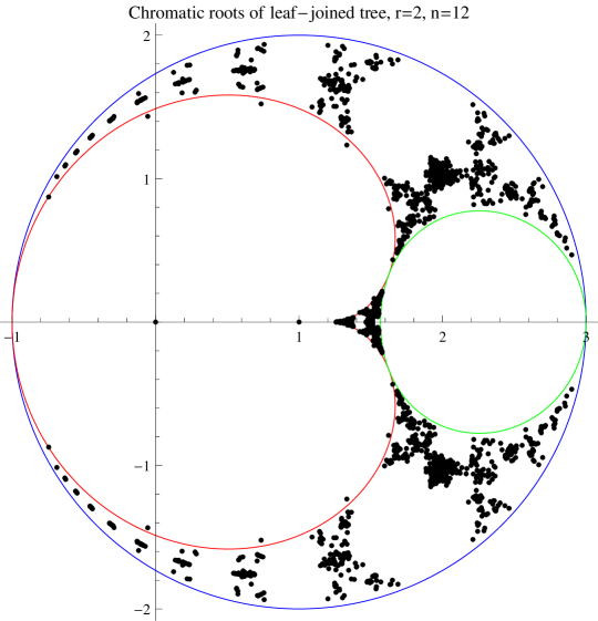
Figure 7: Chromatic roots of the leaf-joined tree $G_{n}^{r}$ with $r=2$ and $n=12$. The blue circle represents the locus $|q-1|=2$ where the fixed point at $y=1$ becomes marginal. The red cardioid represents the locus (B.20) with $|\lambda|=1$, where the fixed point (B.21) becomes marginal. The green egg-shaped curve represents the $q$-plane locus corresponding to (B.22) with $|\lambda|=1$, where the period-2 orbit becomes marginal.

In Figure 7 we plot the chromatic roots of the graph $G_{n}^{r}$ with $r=2$ and $n=12$. The blue circle represents the locus $|q-1|=2$ where the fixed point at $y=1$ becomes marginal. The red cardioid represents the locus (B.20) with $|\lambda|=1$, where the fixed point (B.21) becomes marginal; the cusp of this cardioid lies at $q=5/4$. The green egg-shaped curve represents the $q$-plane locus corresponding to (B.22) with $|\lambda|=1$, where the period-2 orbit becomes marginal. The convergence of the chromatic roots to the circle $|q-1|=2$, as asserted in Theorem B.1, seems quite slow (perhaps like $1/n$). We expect that by a similar argument one can prove convergence of chromatic roots to the red and green curves, but again this convergence seems quite slow.

We see from Figure 7 that all the chromatic roots lie in the region $|q-1|<2$; and we have confirmed this for $n\leq 12$. Let us formulate this as an explicit conjecture for general $r$:

Conjecture B.12

For every $r\geq 2$ and $n\geq 1$, all the chromatic roots of the graph $G_{n}^{r}$ (the leaf-joined tree of branching factor $r$ and height $n$) lie in the disc $|q-1|<r$.

This conjecture can be rephrased as saying that the region $|q-1|\geq r$ where the fixed point at $y=1$ is attractive or marginal is free of chromatic roots.

For $r=2$ it also appears that no chromatic roots lie on or inside the green egg-shaped curve, i.e. in the region where the period-2 orbit is attractive or marginal. We have confirmed this also for $n\leq 12$.

References

- [1] A. Avila and A.D. Sokal, Iteration of holomorphic families of holomorphic maps, in preparation.
- [2] R. Bamón and J. Bobenrieth, The rational maps have no Herman rings, Proc. Amer. Math. Soc. 127, 633–636 (1999).
- [3] A.F. Beardon, Iteration of Rational Functions (Springer-Verlag, New York, 1991).
- [4] M.W. Bern, E.L. Lawler and A.L. Wong, Linear-time computation of optimal subgraphs of decomposable graphs, J. Algorithms 8, 216–235 (1987).
- [5] N.L. Biggs, R.M. Damerell and D.A. Sands, Recursive families of graphs. J. Combin. Theory B 12, 123–131 (1972).
- [6] D.A. Bini and G. Fiorentino, Numerical computation of polynomial roots using MPSolve version 2.2 (January 2000). Software package and documentation available for download at http://www.dm.unipi.it/cluster-pages/mpsolve/
- [7] D.A. Bini and G. Fiorentino, Design, analysis, and implementation of a multiprecision polynomial rootfinder, Numer. Algorithms 23, 127–173 (2000).
- [8] G.D. Birkhoff and D.C. Lewis, Chromatic polynomials, Trans. Amer. Math. Soc. 60, 355–451 (1946).
- [9] J.R. Bobenrieth, Algunos aspectos de la dinámica de las funciones racionales , Ph.D. thesis, Universidad de Chile (June 1997).
- [10] J. Bobenrieth, Hyperbolicity is dense in the real family (), where is odd, Scientia, Series A, Mathematical Sciences (N.S.) 7, 7–11 (2001).
- [11] J. Bobenrieth, Parabolic perturbation in the family , Proyecciones 21, 1–7 (2002).
- [12] J. Bobenrieth, Hyperbolic components of the family , preprint (2000).
- [13] H.L. Bodlaender and B. van Antwerpen-de Fluiter, Parallel algorithms for series parallel graphs and graphs with treewidth two, Algorithmica 29, 534–559 (2001).
- [14] C. Borgs, Absence of zeros for the chromatic polynomial of bounded degree graphs, Combin. Probab. Comput. 15, 63–74 (2006).
- [15] R.B. Borie, R.G. Parker and C.A. Tovey, Automatic generation of linear-time algorithms from predicate calculus descriptions of problems on recursively constructed graph families, Algorithmica 7, 555–581 (1992).
- [16] A. Brandstädt, V.B. Le and J.P. Spinrad, Graph Classes: A Survey (SIAM, Philadelphia, 1999).
- [17] J.V. Brawley, S. Gao and D. Mills, Associative rational functions in two variables, in Finite Fields and Applications, edited by Dieter Jungnickel and Harald Niederreiter (Springer-Verlag, Berlin, 2001), pp. 43–56.
- [18] F. Brenti, G.F. Royle and D.G. Wagner, Location of zeros of chromatic and related polynomials of graphs, Canad. J. Math. 46, 55–80 (1994).
- [19] L. Carleson and T.W. Gamelin, Complex Dynamics (Springer-Verlag, New York, 1993).
- [20] C.J. Colbourn, The Combinatorics of Network Reliability (Clarendon Press / Oxford University Press, New York, 1987).
- [21] R.M. Corless, G.H. Gonnet, D.E.G. Hare, D.J. Jeffrey and D.E. Knuth, On the Lambert function, Adv. Comput. Math. 5, 329–359 (1996).
- [22] R.J. Duffin, Topology of series-parallel graphs, J. Math. Anal. Appl. 10, 303–318 (1965).
- [23] E.J. Farrell, Chromatic roots — some observations and conjectures, Discrete Math. 29, 161–167 (1980).
- [24] R. Fernández and A. Procacci, Regions without complex zeros for chromatic polynomials on graphs with bounded degree, Combin. Probab. Comput. 17, 225–238 (2008). Also available at http://arxiv.org/abs/0704.2617
- [25] G. Grimmett, The Random-Cluster Model (Springer-Verlag, Berlin, 2006).
- [26] B. Jackson, Zeros of chromatic and flow polynomials of graphs, J. Geom. 76, 95–109 (2003). Also available at http://arxiv.org/abs/math/0205047
- [27] B. Jackson, A. Procacci and A.D. Sokal, Complex zero-free regions at large for multivariate Tutte polynomials (alias Potts-model partition functions) with general complex edge weights, J. Combin. Theory B 103, 21–45 (2013). Also available at http://arxiv.org/abs/0810.4703v2
- [28] B. Jackson and A.D. Sokal, Zero-free regions for multivariate Tutte polynomials (alias Potts-model partition functions) of graphs and matroids, J. Combin. Theory B 99, 869–903 (2009). Also available at http://arxiv.org/abs/0806.3249
- [29] B. Jackson and A.D. Sokal, Maxmaxflow and counting subgraphs, Electron. J. Combin. 17 (2010), #R99. Also available at http://arxiv.org/abs/math/0703585v2
- [30] M.Y. Lyubich, An analysis of the stability of the dynamics of rational functions, Selecta Math. Sovietica 9, 69–90 (1990). [Originally published in Russian in Teor. Funktsiĭ Funktsional. Anal. i Prilozhen. 42, 72–91 (1984).]
- [31] J. Milnor, Geometry and dynamics of quadratic rational maps, with an appendix by the author and Lei Tan, Experiment. Math. 2, 37–83 (1993).
- [32] J. Milnor, On rational maps with two critical points, Experiment. Math. 9, 481–522 (2000).
- [33] J. Milnor, Dynamics in One Complex Variable, 3rd ed., Annals of Mathematics Studies #160 (Princeton University Press, Princeton NJ, 2006).
- [34] J. Oxley, Graphs and series-parallel networks, in Theory of Matroids, edited by Neil White (Cambridge University Press, Cambridge, 1986), Chapter 6, pp. 97–126.
- [35] J.G. Oxley, Matroid Theory (Oxford University Press, New York, 1992).
- [36] Q.I. Rahman and G. Schmeisser, Analytic Theory of Polynomials (Clarendon Press / Oxford University Press, Oxford, 2002).
- [37] G. Royle and A.D. Sokal, The Brown–Colbourn conjecture on zeros of reliability polynomials is false, J. Combin. Theory B 91, 345–360 (2004). Also available at http://arxiv.org/abs/math/0301199
- [38] G.F. Royle, Recent results on chromatic and flow roots of graphs and matroids, in Surveys in Combinatorics, 2009, edited by Sophie Huczynska, James D. Mitchell and Colva M. Roney-Dougal (Cambridge University Press, Cambridge–New York, 2009), pp. 289–327.
- [39] W. Rudin, Function Theory in Polydiscs (W.A. Benjamin, New York–Amsterdam, 1969).
- [40] J. Salas and A.D. Sokal, Chromatic roots of the complete bipartite graphs, in preparation.
- [41] A.D. Scott and A.D. Sokal, The repulsive lattice gas, the independent-set polynomial, and the Lovász local lemma, J. Stat. Phys. 118, 1151–1261 (2005). Also available at http://arxiv.org/abs/cond-mat/0309352
- [42] R. Shrock and S.-H. Tsai, Ground-state degeneracy of Potts antiferromagnets: cases with noncompact boundaries having multiple points at , J. Phys. A: Math. Gen. 31, 9641–9665 (1998). Also available at http://arxiv.org/abs/cond-mat/9810057
- [43] R. Shrock and S.-H. Tsai, Ground-state degeneracy of Potts antiferromagnets: homeomorphic classes with noncompact boundaries, Physica A 265, 186–223 (1999). Also available at http://arxiv.org/abs/cond-mat/9811410
- [44] A.D. Sokal, Bounds on the complex zeros of (di)chromatic polynomials and Potts-model partition functions, Combin. Probab. Comput. 10, 41–77 (2001). Also available at http://arxiv.org/abs/cond-mat/9904146
- [45] A.D. Sokal, Chromatic roots are dense in the whole complex plane, Combin. Probab. Comput. 13, 221–261 (2004). Also available at http://arxiv.org/abs/cond-mat/0012369
- [46] A.D. Sokal, The multivariate Tutte polynomial (alias Potts model) for graphs and matroids, in Surveys in Combinatorics, 2005, edited by Bridget S. Webb (Cambridge University Press, Cambridge–New York, 2005), pp. 173–226. Also available at http://arxiv.org/abs/math/0503607
- [47] J.P. Spinrad, Efficient Graph Representations (American Mathematical Society, Providence RI, 2003).
- [48] N. Steinmetz, Rational Iteration (de Gruyter, Berlin, 1993).
- [49] C. Thomassen, The zero-free intervals for chromatic polynomials of graphs, Combin. Probab. Comput. 6, 497–506 (1997).
- [50] J. Valdes, R.E. Tarjan and E.L. Lawler, The recognition of series parallel digraphs, SIAM J. Comput. 11, 298–313 (1982).
- [51] D.G. Wagner, Zeros of reliability polynomials and -vectors of matroids, Combin. Probab. Comput. 9, 167–190 (2000). Also available at http://arxiv.org/abs/math/9802047