A New Mathematical Model for Evolutionary Games on Finite Networks of Players

Abstract

A new mathematical model for evolutionary games on graphs is proposed to extend the classical replicator equation to finite populations of players organized on a network with generic topology. Classical results from game theory, evolutionary game theory and graph theory are used. More specifically, each player is placed in a vertex of the graph and he is seen as an infinite population of replicators which replicate within the vertex. At each time instant, a game is played by two replicators belonging to different connected vertices, and the outcome of the game influences their ability of producing offspring. Then, the behavior of a vertex player is determined by the distribution of strategies used by the internal replicators. Under suitable hypotheses, the proposed model is equivalent to the classical replicator equation. Extended simulations are performed to show the dynamical behavior of the solutions and the potentialities of the developed model.

Keywords: replicator equation on graph, evolutionary game theory, finite populations, complex networks.

1 Introduction

In mathematical literature, there are important examples of models designed to describe the dynamical interaction between a set of players in a game-like context [1, 2, 3, 4]. Players are undistinguishable members of a large population, characterized by a phenotype which determines the fixed strategy they choose among the $M$ available, when playing with any other individual randomly selected in the population.

The payoff earned in the game by each player depends on the elements of a game-specific payoff matrix, while the system dynamics is described by an ordinary differential equation defined in the N-simplex, namely the replicator equation [5, 6].
The solutions of the replicator equation may evolve towards evolutionary stable strategies, which are Nash equilibria of the game and asymptotically stable stationary states [7]. Evolutionary stable strategies are robust against invasion by competing strategies [8, 6]. Other kind of Nash equilibria can also exist, such as equilibria corresponding to Lyapunov stable stationary states of the replicator equation [9].

Replicator equation has been used to describe several phenomena, such as biological evolution driven by replication and selection [10], and reaction-diffusion dynamics [11, 12]. Replicator dynamics including mutation have been studied in [2] and may lead to more complex behaviors, characterized by Hopf bifurcation and limit cycles [13, 14]. Moreover, the replicator equation has been used for solving decision and consensus control problems [15, 16] and machine learning for optimization [17]. Significant application have been also developed in the field of social science [18]. Although widespread, the replicator equation is grounded on several strong assumptions on the system under investigation.

1. The population is very large. Indeed, dominating strategies emerge due to higher rates of replication than the others, causing the frequency of less efficient strategies to become irrelevant in the total population.

2. Any member of the population can play with any other member with the same probability. Participants of each game are chosen randomly and no social structures are present in the population.

3. The payoff earned by each player is defined by the payoff matrix, which is unique for all the population. In some cases, two or more subpopulations with different payoff matrices are considered [19].

4. Players are constrained to behave according to a single fixed strategy at each round of the game they are playing. For instance, if the phenotype of an individual is to be aggressive or generous, he will show the same level of aggressiveness or generosity in any situation at any time, without having the capacity of regulating the level of his natural impulses.

The above assumptions are the basis of the well known equivalence between the replicator equation and some ecological models, such as the predator-prey model introduced by Lotka and Volterra [5].

Several modifications have been introduced in the replicator equation to overcome the limitations caused by the above assumptions. For example, in [18] is presented a generalization of the replicator equation to $N$ players. Concerning networked populations, many efforts have been done to include the topology of connections between players in [21, 20, 2, 22, 23] to deal with scenarios in which the connection between agents plays a fundamental role and may yield to the interpretation of inspected phenomena. For example, in [21] is proposed an algorithm that uses the connections among players and specific updating rules to induce cooperative behavior in an evolutionary prisoner dilemma game. On the other hand, a seminal paper by Ohtsuki et al. [24] presented the replicator equation on infinite graphs, under the assumption that every vertex is connected to the same number of neighbours. In particular, he showed that the replicator equation on a graph with fixed degree is equivalent to a classical replicator equation when the degree goes to infinity.

In this paper, we derive a suitable mathematical model to describe static and dynamical behaviour of an $N$-players game interaction, where an agent is meant to engage his challenges only with a restricted set of players connected to him. To this aim, we make use of the standard non-cooperative game theory results and graph theory. The results presented in the paper generalize many assumptions under the classical replicator equation and recent results on the replicator equation on graphs. Specifically, the equation derived in this paper meets the following:

1. A finite (even small) or infinite population is considered.

2. The elements of the population are the vertices of a graph. Each element can be engaged in a game with another element only if they are connected in the graph. No constraints on the topology of the graph are assumed. Moreover, the connections can be weighted to remark different perceived importance of each interaction.

3. The payoff matrix can be player-specific, including the situations where the perception of the game is different for each individual.

4. Each player can behave according to a combination of strategies. He is a sort of ”mixed player”, thus incorporating composite and multiple personality traits. His behavior can be driven contemporarily by heterogeneous impulses with different strengths, such as, for example, being cooperative and non cooperative, generous and selfish, at the same time. The proposed approach makes players more realistic than in the classical framework and naturally extends the evolutionary game theory to a social context with human players.

The new framework presented in the paper generalizes the classical replicator equation, that can be obtained as a special case by assuming that any individual of the population possesses the same payoff matrix and starts playing from an identical initial condition.

The paper is structured as follows. Section 2 presents some preliminaries on noncooperative games on graphs. Then, the extended version of the replicator equation on graphs with generic topology is introduced in Section 3. Some properties of the new replicator equation are presented in Section 3.2, including the equivalence to the classical replicator equation when homogeneous initial conditions are used. Extended simulations are reported in Section 5, while some conclusions and future work are discussed in Section 6.

2 Non-cooperative games on graphs

In real world situations, interactions between a finite number of rational players can be influenced by topological constraints; in most cases, each player is only able to meet with a reduced number of opponents which are close with respect to a suitable topology, such as the distance between them. In this sense, we talk about networks of players, where interconnections depend on the context. An interesting case of interaction is represented by non-cooperative games, extensively studied in [3, 7].

In this section, we extend the classical game theory by introducing a network, represented by a graph, which describes the connection among the involved players.

2.1 Preliminaries about games on graphs

Typically, networks are described by means of graphs, and in a game context, each player is represented by a vertex. An edge between two players indicates that they interact. However, a player can consider that some interactions are more important than others. Moreover, two connected players can have different perception of the importance of their interaction. These aspects can be accounted by assuming that the graph is weighted and directed; an edge starting from a player and ending to another, is labeled with a positive weight to indicate the importance that the first player attributes to the game.

Formally, let $\mathcal{G}$ be a directed weighted graph of order $N<+\infty$, and let $\mathcal{V}$ be the set of vertices (players) ($\mathcal{V}=\{1,\ldots,N\}$). The graph $\mathcal{G}$ is fully described by its adjacency matrix $\boldsymbol{A}\in\mathbb{R}_{+}^{N\times N}$; in particular, when player $v$ is meant to play with player $w$, then there is an edge which starts from $v$ and ends to $w$. In this case, $(v,w)$-entry of $\boldsymbol{A}$, $a_{v,w}$, is the positive weight attributed by $v$ to the game against $w$. When $a_{v,w}>0$ and $a_{w,v}=0$, there is an interaction between $v$ and $w$, but only $v$ will get a payoff after the challenge. Finally, if both $a_{v,w}$ and $a_{w,v}$ are equal to $0$, then there is no interaction between these players. In general, $a_{v,w}\neq a_{w,v}$. We assume that $\mathcal{G}$ has no self-edge, which means that no player has interaction with himself (i.e. $a_{v,v}=0~{}~{}\forall v\in\mathcal{V}$). We indicate with $\mathcal{N}_{v}=\{w\in\mathcal{V}:a_{v,w}>0\vee a_{w,v}>0\}$ the neighborhood of $v$ (i.e. the set of vertices that interact with $v$), and with $\mathcal{N}^{+}_{v}=\{w\in\mathcal{V}:a_{v,w}>0\}$ the out-neighborhood of $v$ (i.e. the set of vertices $v$ is connected to with and exiting edge). The cardinalities of these set are indicated with $\delta_{v}$ and $\delta^{+}_{v}$, and they represent the degree and out-degree of $v$ respectively. Note that, in general, $\mathcal{N}^{+}_{v}\subseteq\mathcal{N}_{v}$, and also $\delta^{+}_{v}\leq\delta_{v}$.

A player $v$ will play exactly $\delta_{v}$ two-players games with all its neighbours. In each one-to-one competition, the set of available strategies for both players is $\mathcal{S}=\{1,\ldots,M\}$, while the outcome that player $v$ can obtain is defined by a payoff matrix $\boldsymbol{B}_{v}\in\mathbb{R}^{M\times M}$; when player $v$ uses strategy $s\in\mathcal{S}$ in a two-players game against a player which uses strategy $r\in\mathcal{S}$, then he earns a payoff equal to the $(s,r)$-entry of $\boldsymbol{B}_{v}$, $b_{v,s,r}=\boldsymbol{e}_{s}^{T}\boldsymbol{B}_{v}\boldsymbol{e}_{r}$, where $\boldsymbol{e}_{s}$ and $\boldsymbol{e}_{r}$ are the $s$-th and $r$-th versors of $\mathbb{R}^{M}$, respectively.

Each player decides to use the same strategy $s\in\mathcal{S}$ in all the games he is involved in. He will play against all vertices in $\mathcal{N}_{v}$, but he will earn a payoff only when he plays with a player $w\in\mathcal{N}^{+}_{v}$, since when $a_{v,w}=0$ and $a_{w,v}>0$, there is an interaction which is meaningful only for player $w$.

2.2 Effective payoff for games on graphs

In an interconnected context, the effective payoff earned (or the fitness of a strategy) must be defined as an environmental measure depending on all the interactions between near players. This measure must quantify how well a strategy behaves. Since each connection between two players has a positive weight, we pose that the effective payoff for a generic player $v$ is the weighted average of all obtained payoffs. Let’s denote with $s_{w}\in\mathcal{S}$ the strategy of the generic player $w$. Then, the effective payoff of player $v$, $\pi_{v}(s_{1},\ldots,s_{N})$ is the following:

$$\displaystyle\pi_{v}(s_{1},\ldots,s_{N}) = \displaystyle\frac{1}{d_{v}}\sum_{w\in\mathcal{N}^{+}_{v}}\boldsymbol{e}_{s_{v}}^{T}\boldsymbol{B}_{v}\boldsymbol{e}_{s_{w}}=$$ (1)

$$= \displaystyle\boldsymbol{e}_{s_{v}}^{T}\boldsymbol{B}_{v}\left(\frac{1}{d_{v}}\sum_{w=1}^{N}a_{v,w}\boldsymbol{e}_{s_{w}}\right),$$

where $d_{v}=\sum_{w=1}^{N}a_{v,w}$ is the normalization factor. This model of payoff based on weighted average will be denoted with WA. However, there are situations in which payoffs are cumulative and the weighted sum is used without the normalization factor $d_{v}$. In this case we have that:

$$\displaystyle\pi_{v}(s_{1},\ldots,s_{N}) = \displaystyle\sum_{w\in\mathcal{N}^{+}_{v}}\boldsymbol{e}_{s_{v}}^{T}\boldsymbol{B}_{v}\boldsymbol{e}_{s_{w}}=$$ (2)

$$= \displaystyle\boldsymbol{e}_{s_{v}}^{T}(d_{v}\boldsymbol{B}_{v})\left(\frac{1}{d_{v}}\sum_{w=1}^{N}a_{v,w}\boldsymbol{e}_{s_{w}}\right).$$

The payoff model based on weighted sum (WS) can be considered as WA, where each payoff matrix is substituted by $d_{v}\boldsymbol{B}_{v}$. For this reason, we will mainly work on WA model, unless differently specified.

The term $\frac{1}{d_{v}}\sum_{w=1}^{N}a_{v,w}\boldsymbol{e}_{s_{w}}$ that appears in both WA and WS models, is a vector where all components are non-negative numbers which sum up to $1$. In a certain way, player $v$ fights against one virtual player which summarize all the strategies used by its opponents in the set $\mathcal{N}^{+}_{v}$; in general, the strategy used by the virtual player is a mixed strategy which represents what player $v$ effectively sees around him. This aspect will be deeply investigated later in this paper, because it plays a fundamental role to reach our aim.

2.3 $(N-M)$-games and games on graphs

Notice that, for each $v$, $\pi_{v}$ can be interpreted as a $N$-dimensional tensor, where the $(s_{1},\ldots,s_{N})$-entry is $\pi_{v}(s_{1},\ldots,s_{N})$. In this way, the game interaction between interconnected players on a finite graph is equivalent to a $N$-players game, where the set of pure strategies is $\mathcal{S}$, and the payoff of player $v$ is represented by the tensor $\pi_{v}$. The structure of the graph is embedded in this definition, since the payoff tensor depends on the adjacency matrix $\boldsymbol{A}$. Moreover, there are no assumptions made on the structure of the graph itself.

For example, consider the following matrices:

$$\boldsymbol{A}=\left[\begin{array}[]{ccc}0&1&\mu\\ \mu&0&2\mu\\ 0&\mu&0\end{array}\right],~{}~{}\boldsymbol{B}=\left[{}\begin{array}[]{cc}a&b\\ c&d\end{array}\right],$$ (3)

where $\mu\geq 0$, and assume that $\boldsymbol{B}_{v}=\boldsymbol{B}$ for all $v$. In this case, $\mathcal{V}=\{1,2,3\}$ and $\mathcal{S}=\{1,2\}$. Table 1 shows the payoff tensors $\pi_{v}$ of each player, which depend on the model parameters $\mu,a,b,c$ and $d$. Both models WA and WS are considered.

			$\pi_{1}(s_{1},s_{2},s_{3})$		$\pi_{2}(s_{1},s_{2},s_{3})$		$\pi_{3}(s_{1},s_{2},s_{3})$
$s_{1}$	$s_{2}$	$s_{3}$	WA	WS	WA	WS	WA	WS
$1$	$1$	$1$	$a$	$a(1+\mu)$	$a$	$3a\mu$	$a$	$a\mu$
$1$	$1$	$2$	$\frac{a+b\mu}{1+\mu}$	$a+b\mu$	$\frac{a+2b}{3}$	$(a+2b)\mu$	$c$	$c\mu$
$1$	$2$	$1$	$\frac{a\mu+b}{1+\mu}$	$a\mu+b$	$c$	$3c\mu$	$b$	$b\mu$
$1$	$2$	$2$	$b$	$b(1+\mu)$	$\frac{c+2d}{3}$	$(c+2d)\mu$	$d$	$d\mu$
$2$	$1$	$1$	$c$	$c(1+\mu)$	$\frac{2a+b}{3}$	$(2a+b)\mu$	$a$	$a\mu$
$2$	$1$	$2$	$\frac{c+d\mu}{1+\mu}$	$c+d\mu$	$b$	$3b\mu$	$c$	$c\mu$
$2$	$2$	$1$	$\frac{c\mu+d}{1+\mu}$	$c\mu+d$	$\frac{2c+d}{3}$	$(2c+d)\mu$	$b$	$b\mu$
$2$	$2$	$2$	$d$	$d(1+\mu)$	$d$	$3d\mu$	$d$	$d\mu$

Table 1: Payoff tensor of the game on graphs defined by matrices in equation (3) for WA and WS payoff models. For each combination of strategies ($s_{1},s_{2},s_{3}$) the payoffs $\pi_{1},\pi_{2}$ and $\pi_{3}$ of players $1$, $2$, $3$ are reported.

It is evident that the presence of weights, the asymmetry of the matrix, and the use of a particular payoff model may lead to very different calculation of the payoff tensor, and hence, the structure of the game itself changes. Indeed, the effective payoff obtained by a player when he is engaged in a game is essentially evaluated by means of tensors, depending on the adjacency matrix of the graph. These payoffs define the virtual player mentioned at the end of Section 2.2, which embodies all the strategies used by the player’s opponents. As a consequence, each player in the game is a sort of ”mixed player”, thus incorporating composite and multiple personality traits, and behaving according to heterogeneous impulses with different strengths.

As a natural consequence, a $N$-players $M$-strategies game (from now on, $(N,M)$-game) can be extended over the set of mixed strategies $\Delta_{M}$:

$$\Delta_{M}=\{\boldsymbol{z}=[z_{1}\ldots z_{M}]^{T}\in\mathbb{R}^{M}:\sum_{i=1}^{M}z_{i}=1\wedge z_{i}\geq 0~{}~{}\forall i\in\mathcal{S}\}.$$

We indicate with $\boldsymbol{x}_{v}=[x_{v,1}\ldots x_{v,M}]^{T}\in\Delta_{M}$ the mixed strategy of player $v$. Recall that $x_{v,s}$ is the probability that player $v$ uses strategy $s$, while he takes part in the games. The formula of the expected effective payoff that player $v$ obtains, is similar to equation (1):

$$\displaystyle\pi_{v}(\boldsymbol{x}_{1},\ldots,\boldsymbol{x}_{N}) = \displaystyle\frac{1}{d_{v}}\sum_{w\in\mathcal{N}^{+}_{v}}\boldsymbol{x}_{v}^{T}\boldsymbol{B}_{v}\boldsymbol{x}_{w}=$$ (4)

$$= \displaystyle\boldsymbol{x}_{v}^{T}\boldsymbol{B}_{v}\left(\frac{1}{d_{v}}\sum_{w=1}^{N}a_{v,w}\boldsymbol{x}_{w}\right),$$

where $\boldsymbol{x}_{v}^{T}\boldsymbol{B}_{v}\boldsymbol{x}_{w}$ represents the expected outcome for player $v$ of the one-to-one game played by $v$ itself against $w$. From now on, we pose that $\pi_{v}(\boldsymbol{x}_{v},\boldsymbol{x}_{-v})=\pi_{v}(\boldsymbol{x}_{1},\ldots,\boldsymbol{x}_{N})$, where $\boldsymbol{x}_{-v}$ indicates the group of all the vectors $\boldsymbol{x}_{w}$, with $w\neq v$.

When a pure strategy $s$ is used by player $v$, vector $\boldsymbol{x}_{v}$ takes the form of the standard versor $\boldsymbol{e}_{s}$ of $\mathbb{R}^{M}$. If each $\boldsymbol{x}_{w}$ is a versor, say $\boldsymbol{x}_{w}=\boldsymbol{e}_{s_{w}}$, then equations (1) and (4) coincide. Furthermore, we can define the expected payoff $p_{v,s}$ of player $v$ when he is preprogrammed to use the strategy $s$ (hence $\boldsymbol{x}_{v}=\boldsymbol{e}_{s}$) in all games played against its neighbours:

$$\displaystyle p_{v,s} = \displaystyle\pi_{v}(\boldsymbol{e}_{s},\boldsymbol{x}_{-v})=$$ (5)

$$= \displaystyle\boldsymbol{e}_{s}^{T}\boldsymbol{B}_{v}\left(\frac{1}{d_{v}}\sum_{w=1}^{N}a_{vw}\boldsymbol{x}_{w}\right).$$

Equation (5) easily leads to a more convenient definition of the expected payoff obtained by the player $v$. That is:

$$\displaystyle\phi_{v} = \displaystyle\pi_{v}(\boldsymbol{x}_{v},\boldsymbol{x}_{-v})=$$ (6)

$$= \displaystyle\boldsymbol{x}_{v}^{T}\boldsymbol{B}_{v}\left(\frac{1}{d_{v}}\sum_{w=1}^{N}a_{vw}\boldsymbol{x}_{w}\right).$$

The present work uses the same theoretical issues developed in the classical non-cooperative $(N-M)$-games theory ([3, 7, 25]). The differences here introduced, consist with the possibility of embedding any topological structure in the game; indeed, the payoff tensor used to describe the game depends on the adjacency matrix of the graph.

3 The replicator equation on graphs

Thanks to game theory, we are able to predict the strategies of opponents, assuming that all of them behave in a rational way during their decision-making tasks. In fact, rational players choose pure strategies which may lead to a pure Nash equilibrium, whenever it exists. Recall that Nash theorem [7] asserts that a game has always at least one Nash equilibrium within the set of mixed strategies. If the game is repeated over time, we can imagine that a mixed strategy describes, for each time, the probability that a player uses a certain pure strategy independently from the choices made until that moment. Payoff is computed as the average outcome that a player obtains when the game is reiterated for an infinite number of times, and Nash equilibria are evaluated accordingly. Although players’ behavior is randomized over time, there is a precise rational scheme that they follow. Hence, pure and mixed strategies games are quite similar, since in both cases players decide their behaviors through a rational decision-making task at the beginning of the game.

Often, in real world situations, players do not have a full knowledge about the game, and the decision-making process suggested by game theory is not applicable. However, players can learn from the context; time after time, they are able to compare their payoffs with the outcomes of their opponents, and strategies are changed accordingly. For example, after some game iterations, one can understand that its opponent is preprogrammed to play always the same strategy $r$, and then he decides to adopt the strategy $s$ which is the best reply to $r$ (i.e. he obtains the maximum payoff knowing the strategy of his opponent). Also, a player can simply imitate the strongest opponent to reach a greater payoff.

Evolutionary biology gives an interesting interpretation for mixed strategies. Let’s consider a large population in which each individual is programmed to play a particular pure strategy. Population is divided according to a mixed strategy, which indicates the frequency of pure strategies in the population. Pairs of individuals are randomly drawn from the population to play games. The average payoff obtained by all players playing a certain strategy is a measurement of the fitness of that strategy.

Nature promotes fittest strategies; time after time, when a strategy has a payoff greater than average, its frequency must increase, and consequently, frequencies relative to poorly fit strategies decrease. This natural selection process may yield to interesting dynamical phenomena, since the fitness of each strategy changes over time according to the frequencies of the subpopulations. Natural selection is realized through reproduction. Generally, this happens asexually and the offspring produced is identical to parent. For these reasons, a player in this context is also known as replicator. He is preprogrammed to use a certain strategy and there is no rational decision-making process. A strategy is something included in the genes of a replicator, and hence, exhibited from birth. A replicator uses a “good” strategy when has a fitness greater than the average. Nature favors players with a good strategy, by allowing them to survive and to produce offspring.

The dynamics of replicator populations can be used to describe several non-biological situations: scientific ideas, life-styles, political orientations diffuse by means of imitation and education process that easily replace the concept of asexual reproduction. In fact, this becomes clearer if we interpret fitness as a measurement quantifying how well a strategy behaves in a certain context, whatever it is.

3.1 Towards evolutionary $(N-M)$-games

In this section we develop a key idea which leads to the definition of a replicator equation based on a generic graph, where the number of players and the network structure are arbitrary.

Main idea - We imagine that each vertex of the network contains an infinite population of individuals. We will refer to such elements as atomic players, and to vertices of the network as vertex players. The first are replicators, while the latter are the players introduced in paragraph 2.3 for $(N-M)$-games. Basically, each atomic player behaves like the corresponding vertex player: an atomic player of $v$ takes part to $2$-players games, described by payoff matrix $B^{v}$, against exactly one atomic player randomly drawn from each connected vertex, and his effective payoff is the average of the payoffs obtained in all the one-to-one competitions. By the way, atomic players are different from vertex players. Indeed, all atomic players inside a vertex are indistinguishable, except for the fact that each of them is preprogrammed to use a certain pure strategy in $\mathcal{S}$ during all the games he is involved in. On the contrary, vertex players can also adopt mixed strategies. Atomic players reproduce themselves by replication, after their participation to games, inside their population. Furthermore, their capacity to produce offspring is related to the effective payoff obtained.

Assume that one atomic player is randomly draw from each populations, and let $s_{w}$ be the strategy used by the one extracted from population $w$. Then, the effective payoff earned by the atomic player of population $v$ is defined by equation (1). Now, $x_{v,s}$ can be interpreted as the share of atomic players preprogrammed to use the pure strategy $s$ inside the vertex $v$. This implies that $p_{v,s}$ is the expected effective payoff obtained by an atomic player of $v$ when he uses strategy $s$, while $\phi_{v}$ represents the expected effective payoff for a generic atomic player randomly drawn from population $v$ (see equations (5) and (6)). A mixed strategy of a vertex player can be interpreted as the way in which its internal population of atomic players is distributed, according to the pure strategy they are preprogrammed to play.

3.2 Mathematical formulation of the replicator equation on graphs

Suppose now that the games are iterated in time. We will refer to game session as the whole set of $2$-players games performed on the graph. The probability for a replicator to survive and to reproduce himself between two games sessions, depends on the comparison between the effective payoff obtained and the average effective payoff of all other players. Let’s assume that games’ sessions take place at discrete and equidistant times (say, a session after each $\tau$ seconds). Let $x_{v,s}(t)$ indicate the share of population inside vertex $v$, which is preprogrammed to use the pure strategy $s$, at time $t$.

What happens to $x_{v,s}(t+\tau)$? First of all, suppose for a while that the population size in the generic node $v$ at time $t$ is $n_{v}(t)$. According to [6, 1, 2], we can consider that $p_{v,s}(t)$ represents a reproductive rate and therefore, $p_{v,s}(t)\tau$ is the number of offspring produced by one atomic player in $v$ that uses strategy $s$ between $t$ and $t+\tau$. Hence, the population size after a time $\tau$ is equal to the previous size plus the produced offspring, since each atomic player reproduces himself within his population. That is:

$$n_{v}(t+\tau)=n_{v}(t)+\sum_{r=1}^{M}n_{v}(t)x_{v,r}(t)p_{v,r}(t)\tau,$$

where $n_{v}(t)x_{v,r}(t)$ is the size of the subpopulation which uses strategy $r$ at time $t$, and $n_{v}(t)x_{v,r}(t)p_{v,r}(t)\tau$ is the number of offspring produced by this subpopulation. By definition, $x_{v,s}(t+\tau)$ is the ratio between the size of subpopulation $s$ and the total population. Therefore:

$$\displaystyle x_{v,s}(t+\tau) = \displaystyle\frac{n_{v}(t)x_{v,s}(t)+n_{v}(t)x_{v,s}(t)p_{v,s}(t)\tau}{n_{v}(t+\tau)}=$$ (7)

$$= \displaystyle\frac{n_{v}(t)x_{v,s}(t)(1+p_{v,s}(t)\tau)}{n_{v}(t)\left(1+\displaystyle\sum_{r=1}^{M}x_{v,r}(t)p_{v,r}(t)\tau\right)}=$$

$$= \displaystyle\frac{x_{v,s}(t)(1+p_{v,s}(t)\tau)}{1+\phi_{v}(t)\tau}.$$

Notice that equation (7) does not depend on $n_{v}(t)$, and hence this relationship is valid for any starting size of the population.

Our aim is to develop a mathematical model that describes the evolutionary process on a graph when the time between replication events goes to $0$, thus making atomic players able to reproduce themselves continuously in time. Let’s consider the difference ratio of $x_{v,s}(t)$:

$$\frac{x_{v,s}(t+\tau)-x_{v,s}(t)}{\tau}=\displaystyle\frac{x_{v,s}(t)(p_{v,s}(t)-\phi_{v}(t))}{1+\phi_{v}(t)\tau}.$$

Letting $\tau\rightarrow 0$, we obtain that:

$$\dot{x}_{v,s}(t)=x_{v,s}(t)(p_{v,s}(t)-\phi_{v}(t)),$$ (8)

where the “dot” indicates the derivative with respect to time $t$. Finally, we can write the following Cauchy problem:

$$\left\{\begin{array}[]{l}\displaystyle\dot{x}_{v,s}(t)=x_{v,s}(t)(p_{v,s}(t)-\phi_{v}(t))\\ \\ \displaystyle x_{v,s}(0)=c_{v,s}\end{array}\right.~{}~{}\forall v\in\mathcal{V},~{}~{}\forall s\in\mathcal{S},$$ (9)

where, for consistency, it is assumed that the distribution of strategies at the initial time $t=0$ is known for each vertex (i.e. $\boldsymbol{x}_{v}(0)=[c_{v,1}\ldots c_{v,M}]^{T}\in\Delta_{M}$).

Systems (9) represents the replicator equation on a graph. Note that no assumptions on the structure of the graph is needed to derive the equation (8). Indeed, the adjacency matrix of the network is fully embedded in the payoff tensors.

It is straightforward to note that the equation (8) has a structure similar to the classical replicator equation; for example, dominant strategies are the fittest, and hence when the relative fitness $p_{v,s}$ is better than the average $\phi_{v}$, the corresponding frequencies will grow over time. In the next section, the very strong correlation between the two equations will be rigorously shown. Furthermore, the relationship between Nash equilibria of the underlying $(N-M)$-game and the rest points of the dynamical equation (8) will also be discussed in section 4.

4 Properties of the replicator equation on graphs

4.1 Invariance of $\Delta_{M}$

Let $\boldsymbol{x}_{v}(t)$ be the unique solution of problem (9), obtained by posing $\boldsymbol{x}_{v}(0)\in\Delta_{M}$. In addition, suppose that there exists a time instant $t_{2}$ where $x_{v,s}(t_{2})<0$. Since all the components of the solution are continuous and non-negative at $t=0$, then there must be a time $t_{1}<t_{2}$ such that $x_{v,s}(t_{1})=0$. Following equation (8), we can state that $\dot{x}_{v,s}(t_{1})=0$, and hence, this component will be $0$ for all times after $t_{1}$. For the unicity of the solution, this implies that no time $t_{2}$ for which $x_{v,s}(t_{2})<0$ exists. Thus, for each $v\in\mathcal{V}$ we have that:

$$\boldsymbol{x}_{v}(0)\in\Delta_{M}\Rightarrow x_{v,s}(t)\geq 0,$$ (10)

for all strategies $s\in\mathcal{S}$ and for all times $t>0$. Notice that the total variation of the strategies distribution in a vertex is null at time $t$ when $\sum_{s=1}^{M}x_{v,s}(t)=1$. In fact:

$$\displaystyle\sum_{s=1}^{M}\dot{x}_{v,s}(t) = \displaystyle\sum_{s=1}^{M}x_{v,s}(t)(p_{v,s}(t)-\phi_{v}(t))=$$

$$= \displaystyle\sum_{s=1}^{M}x_{v,s}(t)p_{v,s}(t)-\phi_{v}(t)\sum_{s=1}^{M}x_{v,s}(t)=$$

$$= \displaystyle\phi_{v}(t)-\phi_{v}(t)\cdot 1=0.$$

This means that:

$$\sum_{s=1}^{M}x_{v,s}(t)=\sum_{s=1}^{M}x_{v,s}(0)~{}~{}\forall t>0,~{}~{}\forall v\in\mathcal{V}.$$ (11)

Imposing that $\boldsymbol{x}_{v}(0)\in\Delta_{M}$, the last equation asserts that $\sum_{s=1}^{M}x_{v,s}(t)=1$ for all time $t>0$. Joining the results provided by (10) and (11), we conclude the following:

$$\forall v\in\mathcal{V}:\boldsymbol{x}_{v}(0)\in\Delta_{M}\Rightarrow\boldsymbol{x}_{v}(t)\in\Delta_{M}~{}~{}\forall t>0.$$ (12)

In other words, all trajectories that start inside $\Delta_{M}$ remain inside $\Delta_{M}$ itself for all time $t>0$. At any time, $\boldsymbol{x}_{v}(t)$ can be always interpreted as a distribution of strategies.

4.2 Nash equilibria are rest points of the replicator equation on graph

Recall that the best response function for the static $(N-M)$-game is:

$$\begin{array}[]{l}\displaystyle\beta_{v}(\boldsymbol{x}_{-v})=\\ \displaystyle=\left\{\boldsymbol{x}_{v}\in\Delta_{M}:\pi_{v}(\boldsymbol{x}_{v},\boldsymbol{x}_{-v})\geq\pi_{v}(\boldsymbol{z},\boldsymbol{x}_{-v})~{}~{}\forall\boldsymbol{z}\in\Delta_{M}\right\}.\end{array}$$

Suppose that $\boldsymbol{x}^{*}_{1}(t),\ldots\boldsymbol{x}^{*}_{N}(t)$ is a Nash equilibrium. Then:

$$\boldsymbol{x}^{*}_{v}(t)\in\beta_{v}(\boldsymbol{x}^{*}_{-v}(t))$$

for each vertex $v$. This means that:

$$\displaystyle\dot{x}^{*}_{v,s}(t) = \displaystyle x^{*}_{v,s}(t)(p^{*}_{v,s}(t)-\phi^{*}_{v}(t))=$$

$$= \displaystyle x^{*}_{v,s}(t)(\pi_{v}(\boldsymbol{e}_{s},\boldsymbol{x}^{*}_{-v}(t))-\pi_{v}(\boldsymbol{x}^{*}_{v}(t),\boldsymbol{x}^{*}_{-v}(t)))\leq 0$$

Moreover, from (12) we know that:

$$\sum_{s=1}^{M}\dot{x}^{*}_{v,s}(t)=0~{}~{}\forall v\in\mathcal{V},$$

and then:

$$\dot{x}^{*}_{v,s}=0~{}~{}\forall v\in\mathcal{V},~{}~{}\forall s\in\mathcal{S}.$$

We can conclude that every Nash equilibrium is also a rest point of the replicator equation on graph.

4.3 Pure strategies are rest points of the replicator equation on graph

Suppose that $\boldsymbol{x}_{v}(t)=\boldsymbol{e}_{q}$. Then $p_{v,q}(t)=\phi_{v}(t)$ and

$$\dot{x}_{v,q}(t)=x_{v,q}(t)(p_{v,q}(t)-\phi_{v}(t))=1\cdot 0=0.$$

In addition, $x_{v,r}(t)=0$ if $r\neq q$, and again:

$$\dot{x}_{v,r}(t)=x_{v,r}(t)(p_{v,r}(t)-\phi_{v}(t))=0\cdot(p_{v,r}(t)-\phi_{v}(t))=0.$$

For this reason:

$$\boldsymbol{x}_{v}(t)=\boldsymbol{e}_{q}\Rightarrow\dot{x}_{v,s}(t)=0~{}~{}\forall s,q\in\mathcal{S}.$$

This implies that if each $\boldsymbol{x}_{v}(t)$ represents a pure strategy (i.e. it is equal to a versor of $\mathbb{R}^{M}$), then we have a rest point of the replicator equation on graph.

4.4 The classical replicator equation as a special case

Suppose to fix a time lag $\tau>0$, and assume that the mixed strategies are all the same for each vertex and for any time $t_{0}\in[0,\tau)$. That is:

$$\boldsymbol{x}_{v}(t_{0})=\boldsymbol{c}=[c_{1}\ldots c_{M}]^{T}\in\Delta_{M}~{}~{}\forall v\in\mathcal{V},~{}~{}\forall t_{0}\in[0,\tau).$$

Consider the payoff model WA and suppose that $\boldsymbol{B}_{v}=\boldsymbol{B}$ for all vertices $v$. Following equations (5) and (6), we obtain that $p_{v,s}(t_{0})=\boldsymbol{e}_{s}^{T}\boldsymbol{B}\boldsymbol{c}$ and $\phi_{v}(t_{0})=\boldsymbol{c}^{T}\boldsymbol{B}\boldsymbol{c}$. In this case, we can rewrite the difference equation (7) as follows:

$$x_{v,s}(t_{0}+\tau)=\frac{c_{s}(1+\tau\boldsymbol{e}_{s}^{T}\boldsymbol{B}\boldsymbol{c})}{1+\tau\boldsymbol{c}^{T}\boldsymbol{B}\boldsymbol{c}}.$$

Since previous equations do not depend on $v$, we are able to impose that $\boldsymbol{y}(t_{0})=\boldsymbol{x}_{v}(t_{0})$ and $\boldsymbol{y}(t_{0}+\tau)=\boldsymbol{x}_{v}(t_{0}+\tau)$, $\forall v\in\mathcal{V},~{}~{}\forall t_{0}\in[0,\tau)$, and hence:

$$y_{s}(t_{0}+\tau)=\frac{y_{s}(t_{0})(1+\tau\boldsymbol{e}_{s}^{T}\boldsymbol{B}\boldsymbol{y}(t_{0}))}{1+\tau\boldsymbol{y}(t_{0})^{T}\boldsymbol{B}\boldsymbol{y}(t_{0})}.$$

It’s straightforward to note that any other iteration of the previous map leads to quantities that are independent from $v$. For example, applying a second iteration we get that:

$$x_{v,s}(t_{0}+2\tau)=\frac{y_{s}(t_{0}+\tau)(1+\tau\boldsymbol{e}_{s}^{T}\boldsymbol{B}\boldsymbol{y}(t_{0}+\tau))}{1+\tau\boldsymbol{y}(t_{0}+\tau)^{T}\boldsymbol{B}\boldsymbol{y}(t_{0}+\tau)},$$

and hence we can pose that $\boldsymbol{x}_{v}(t_{0}+2\tau)=\boldsymbol{y}(t_{0}+2\tau)$. Generalizing to any time lag, $\boldsymbol{x}_{v}(t_{0}+k\tau)=\boldsymbol{y}(t_{0}+k\tau)$ for any non negative integer $k$. Similarly, $p_{v,s}(t_{0}+k\tau)=\boldsymbol{e}_{s}^{T}\boldsymbol{B}\boldsymbol{y}(t_{0}+k\tau)$ and $\phi_{v}(t_{0}+k\tau)=\boldsymbol{y}(t_{0}+k\tau)^{T}\boldsymbol{B}\boldsymbol{y}(t_{0}+k\tau)$ are also independent from $v$. For these reasons, we pose that $p_{s}(t_{0}+k\tau)=p_{v,s}(t_{0}+k\tau)$ and $\phi(t_{0}+k\tau)=\phi_{v}(t_{0}+k\tau)$. Then, the discrete map becomes the following:

$$y_{s}(t_{0}+(k+1)\tau)=\frac{y_{s}(t_{0}+k\tau)(1+\tau p_{s}(t_{0}+k\tau))}{1+\tau\phi(t_{0}+k\tau)}.$$ (13)

Note that, for any $t\geq 0$ there exist a non-negative integer $k$ and a real number $t_{0}\in[0,\tau)$, with $\tau>0$ fixed, such that $t=t_{0}+k\tau$. Then, equation (13) becomes:

$$y_{s}(t+\tau)=\frac{y_{s}(t)(1+\tau p_{s}(t))}{1+\tau\phi(t)}~{}~{}\forall t\geq 0.$$ (14)

Considering the difference ratio $\frac{1}{\tau}(y_{s}(t+\tau)-y_{s}(t))$, and letting $\tau\rightarrow 0$, we obtain the following differential equation:

$$\dot{y}_{s}(t)=y_{s}(t)(p_{s}(t)-\phi(t)),$$ (15)

which is the classical replicator equation.

This result is quite straightforward if we imagine to divide a wide population of replicators into $N$ subpopulations, assuming that all of them are described by the same mixed strategy of the total one at initial time. Then, each subpopulation will behave exactly as the total one. Hence, the dynamics of a single subpopulation in a vertex can be described by the classical replicator equation applied to the single population, whatever is the graph used.

5 Simulations

In this chapter, we present some simulations produced by equation (8). The $WA$ payoff model is used. In particular, we set up experimental sessions by considering different $2$-strategies payoff matrices ($\mathcal{S}=\left\{1,2\right\}$); it is assumed that every vertex has the same payoff matrix. Each session has been developed over $3$ different graphs with $6$ vertices as reported in Figure 1.

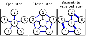
Figure 1: Graphs topologies. All edges have weights equal to $1$, except for thicker ones in the asymmetric weighted graph, having weights equal to $3$.

All edges represented in Figure 1 have the same weight, except for thicker ones in the asymmetric weighted graph. Note that we are using only undirected graphs (i.e. $a_{v,w}=a_{w,v}$). Our aim is to show the behavior of the replicator equation on graphs when initial players strategies are almost pure. In fact, a vertex player with a pure strategy is in steady state; for this reason, initial conditions used for vertex players are equals to slightly perturbed pure strategies (i.e. $[0.99~{}0.01]^{T}$ and $[0.01~{}0.99]^{T}$ are used in place of pure strategies $1$ and $2$, respectively). Replicator equation on graphs has been simulated until a steady state behavior is reached, starting from $4$ different distribution initial conditions on the graph.

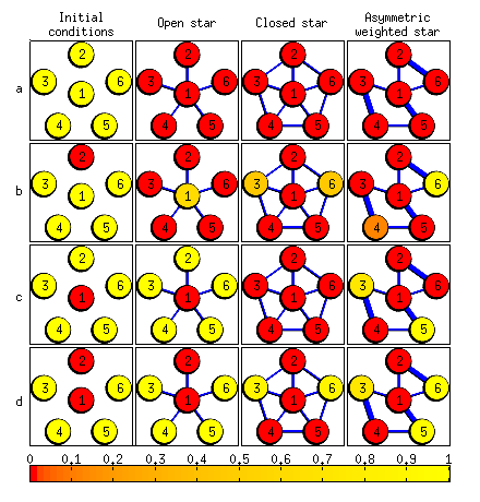
Figure 4: Strategies distribution at $t=0$ (first column) and at $t=100$ (other columns) on open, closed and asymmetric weighted star graphs, when the payoff matrix is reported in equation (17) and $\theta=1.5$. $4$ different initial conditions are considered: homogeneous (a), external outlayer (b), central outlayer (c) and external-central outlayers (d).

The steady state situations are shown in Figures 2, 3, 4 and 6. The first column of each Figure gives a picture of the initial conditions used, while others report the solution of the simulations when steady state is reached for each of the considered graphs. The color of each vertex indicates the value of $x_{v,1}$, and hence it visually quantifies the inclination of player $v$ toward one of the $2$ feasible pure strategies; yellow is used for player with strategy $1$ ($x_{v,1}=1$), red is for strategy $2$ ($x_{v,1}=0$). Mixed strategies ($0<x_{v,1}<1$) are indicated by shaded colors, according to the color bar at the bottom of the Figures. Moreover, Figures 5 and 7 report the dynamical evolution obtained on the asymmetric weighted graph; the same initial condition is used in both Figures, while payoff matrices are different. The following sections will discuss in detail the results of each simulation.

5.1 Two pure Nash equilibria

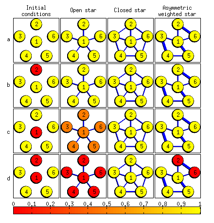
Figure 2: Strategies distribution at $t=0$ (first column) and at $t=50$ (other columns) on open, closed and asymmetric weighted star graphs, when the payoff matrix is reported in equation (16) and $\theta=1$. $4$ different initial conditions are considered: homogeneous (a), external outlayer (b), central outlayer (c) and external-central outlayers (d).

In this first experimental session, we used the following payoff matrix:

$$\boldsymbol{B}=\left[\begin{array}[]{cc}1&0\\ 0&\theta\end{array}\right],$$ (16)

with $\theta>0$.

The $2$-players game described by $\boldsymbol{B}$ has $2$ strict pure Nash equilibria (i.e. both players use strategy $1$ or $2$) and a mixed Nash equilibrium

$$\boldsymbol{x}^{*}=\left[\frac{\theta}{1+\theta}~{}~{}\frac{1}{1+\theta}\right]^{T}.$$

The classical replicator equation, based on matrix $\boldsymbol{B}$, has exactly $3$ rest points which coincide with the Nash equilibria reported above. Moreover, mixed equilibrium is repulsive, while pure equilibria are attractive; for this reason, we say that $B$ is a bistable payoff matrix.

Figure 2 reports some results obtained when $\theta=1$. Row (a) of the Figure shows what happens when an homogeneous initial condition is used; as said in section 4.4, the dynamics is the same for each vertex player, and it is equivalent to the solution given by the classical replicator equation, whichever is the underlying graph structure. After a certain time, all vertex players adopt pure strategy $1$, since it represents an attractive rest point, and initial condition is in inside the relative basin of attraction.

In the row (b) of Figure 2 are reported the steady state situations obtained by using an homogeneous initial condition, where only one peripheral player uses the quasi-pure strategy $2$. At the end of simulation, the pure strategy $1$ spreads all over the considered graphs. Let’s consider the open graph situation: the vertex player $1$, which is the unique neighbors of player $2$, has no will to change his own strategy, since he is surrounded by $4$ yellow players. Similarly, on the closed and asymmetric weighted star, neighbors of player $2$ see an equivalent player which is almost yellow. Thus, none of them wants to change, and player $2$ must modify his strategy. Hence player $2$ must change his strategy to obtain a good payoff. In a certain way, the ”rebel“ peripheral player decides to adapt himself to the majority.

The dynamical behavior is slightly different when the central hub is the rebel. In the row (c) of the Figure 2 are shown the solutions of the replicator equation on graphs for this initial condition. When the open star is used, player $1$ sees a yellow equivalent player, while all peripheral players have only him as neighbor. Player $1$ decides to change his own strategy to yellow, while all others do the exact opposite. After a certain time, they meet half way, at the mixed equilibrium $[0.5~{}0.5]^{T}$. The different position of the rebel player in the graph influences a lot the dynamics of the whole system; the leader (player $1$) understands that he must modify his own strategy according to his neighborhood, while all other players do the same, since their only opponent is player $1$ himself. However, closed and asymmetric weighted graphs are more resistant to the influence of player $1$, because the peripheral players have more than one neighbors; in these situations, player $1$ does not play anymore as a leader able to change the whole dynamics.

The last row (d) of Figure 2 reports the final solutions when both player $1$ and $2$ use the quasi-pure strategy $2$. While the closed star structure remains resistant to the influence of rebel players, the other graphs do not. The open star becomes all red at final time. This is because player $2$ sees only player $1$: they are both red, so player $2$ doesn’t want to change strategy. Simultaneously, yellow neighbors of $1$ change their strategy to red, since they see only a red player.

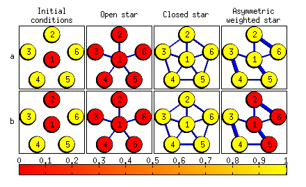
Figure 3: Strategies distribution at $t=0$ (first column) and at $t=50$ (other columns) on open, closed and asymmetric weighted star graphs, when the payoff matrix is reported in equation (16) and $\theta=1.1$. $2$ different initial conditions are considered: central outlayer (a) and external-central outlayers (b).

Changing the value of the parameter $\theta$ leads to different behaviors. When $\theta<1$, first strategy becomes stronger and it spreads all over the considered graphs as $\theta$ goes to $0$. In Figure 3 are reported some results obtained with $\theta=1.1$. In particular, when player $1$ uses strategy $2$ at the beginning, then mixed equilibrium is not reached anymore on the open star graph; all vertices adopt strategy $2$, which is slightly better than strategy $1$. The strength of strategy $2$ is also visible on the asymmetric weighted star, when at the beginning both player $1$ and $2$ adopt strategy $2$; in Figure 2 ($\theta=1$) we have shown that on steady state, players $2$ and $6$ are the only ones red, while when $\theta=1.1$, also players $1$ and $5$ do. In general, when $\theta>1$, strategy $2$ becomes stronger and it spreads all over the considered graphs as $\theta$ grows up.

5.2 Prisoners’ dilemma

In this section, we show the results obtained with the replicator equation on graphs, by using a modified version of the prisoners’ dilemma game, as proposed in [2]. The payoff matrix is the following:

$$\boldsymbol{B}=\left[\begin{array}[]{cc}1&0\\ \theta&0\end{array}\right],$$ (17)

where $\theta>1$.

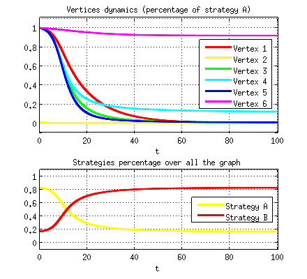
Figure 5: Prisoners’ dilemma game. Time courses of each vertex (top) and average behavior over the network (bottom). Network topology, initial conditions and parameter $\theta$ are the same used in Figure 4, row b, column 4.

Cooperate and Defect are the names typically used to indicate, respectively, the strategy $1$ and $2$ of this classic game. The dilemma is that mutual cooperation produces a better outcome than mutual defection; however, at the individual level, the choice to cooperate is not rational from a selfish point of view. In other words, the $2$-players game has only one Nash equilibrium, reached when both players defect. Note that in this version of the prisoner’s dilemma, the Nash equilibrium is non strict. Moreover, classical replicator equation based upon payoff matrix reported in equation (17), has $2$ rest points, which correspond to the pure strategies $(1,1)$ and $(2,2)$. In particular, the first one is repulsive, while the latter is attractive.

Although mutual defection represents both a Nash and a dynamical equilibrium, many works have shown that cooperation does not vanishes when games are played over graphs and $\theta$ is equal to suitable values (see [22, 2, 20, 21]). The resilience of cooperation is shown in 4, where $\theta$ is set to $1.5$. Steady states depend on the initial conditions and on the type of graph used, and behaviors can be very heterogeneous. When an homogeneous initial condition is considered (row (a)), all players on graphs become defectors (again, this is the case when the classical and proposed replicator equations are the same). On the other side, when initial conditions are not homogeneous (rows (b), (c) and (d)), cooperation does not always completely vanish. Figure 5 shows the time course of the variable $x_{v,1}$ for each vertex of the graph. In particular, the initial conditions with external outlayer and the asymmetric weighted graph have been used.

5.3 Unique mixed Nash equilibrium

In some $2$-players games there are no pure Nash equilibria. Nevertheless, Nash theorem guarantees that at least a mixed equilibrium exists. For example, this happens when payoff matrix is defined as follows:

$$\boldsymbol{B}=\left[\begin{array}[]{cc}0&1\\ 1&0\end{array}\right].$$ (18)

The unique mixed Nash equilibrium is:

$$\boldsymbol{x}^{*}=\left[0.5~{}~{}0.5\right]^{T}.$$

Classical replicator equation has $3$ rest points; symmetric couples of pure strategies, $(1,1)$ and $(2,2)$ are repulsive, while the mixed equilibrium is attractive. In this case, we speak about $coexistence$ of both feasible strategies.

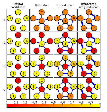
Figure 6: Strategies distribution at $t=0$ (first column) and at $t=50$ (other columns) on open, closed and asymmetric weighted star graphs, when the payoff matrix is reported in equation (18). $4$ different initial conditions are considered: homogeneous (a), external outlayer (b), central outlayer (c) and external-central outlayers (d).

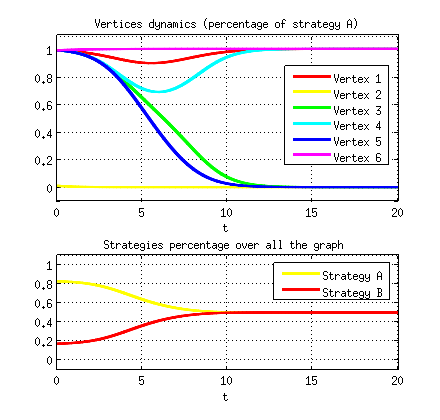
Figure 7: Unique mixed Nash equilibrium game. Time courses of each vertex (top) and average behavior over the network (bottom). Network topology and initial conditions are the same used in Figure 6, row b, column 4.

In Figure 6 the steady state solutions when payoff matrix defined in equation (18) is used, are reported. Again, when we have an homogeneous initial condition, everything works like a classical replicator equation, and hence, all players go to the mixed Nash equilibrium. When initial condition is not homogeneous, behaviors obtained through the replicator equation on graphs are strongly based on the topological structure of the underlying graph and on the initial conditions. Figure 7 shows in details the behavior of the population when the asymmetric weighted graph and initial conditions with external outlayer are supposed.

6 Conclusions

In this work a new mathematical model for evolutionary games on graphs with generic topology has been developed. We proposed a replicator equation on graphs,dealing with a finite population of players connected through an arbitrary topology. A link between two players can be weighted by a positive real number to indicate the strength of the connection. Furthermore, the different perception that each player has about the game is modeled by allowing the presence of directed links and different payoff matrices for each member of the population. A player obtains his outcome after $2$-players games are played with his neighbors; payoffs of each game are averaged (WA model) or simply summed up (WS model). Moreover, it has been shown that the proposed replicator equation on graphs extends the classical one, under the hypotheses that WA model for payoffs is used, homogeneous initial conditions over the vertices are considered, all vertex players have the same payoff matrix. In any case, no limitations are imposed to the underlying graph.

Experimental results showed that the dynamics of evolutionary games are strongly influenced by the network topology. As expected, more complex behavior emerges with respect to the classical replicator equation. For example, in the prisoner’s dilemma game, cooperative and non-cooperative behaviors can coexist over the graph. Moreover, when a $2$-player game with strictly dominant strategies is considered, heterogeneous behavior is obtained, i.e. a part of the population chooses to play a dominant strategy, while others use different strategies. Then, players become mixed (coexistence of strategies).

The very first step for extending this work is the study of dynamical and evolutionary stability of the rest points. By the way, we imagine that the concept of evolutionary stability must be revisited to deal with the proposed evolutionary multi-players game model based on graph, for which a theoretical effort is needed. Indeed, in our opinion, the basic question “is strategy $s$ resistant to invasion?” must be reformulated to fit with the new model, where the population of players is finite and is organized according to a social structure.

The theory developed in this paper can also be extended to 3 or more strategies and can consider more complex topologies of the graph, such as small world, scale free, and random complex networks.
From an applicative point of view, the authors intend to use the replicator equation on graphs to deal with biological and physical processes, such as bacterial growth [26], model of brain dynamics [27] and reaction-diffusion phenomena [28]. The developed model can be also profitably applied to solve networked socio-economics problems, such as decision making for the development of marketing strategies.

References

- [1] J. Hofbauer and K. Sigmund, Evolutionary game dynamics, Bull. Am. Math. Soc., 40, pp. 479-519, 2003.
- [2] M. Nowak, Evolutionary Dynamics: Exploring the Equations of Life, Belknap Press of Harvard University Press. 2006.
- [3] J. von Neumann, 0. Morgenstern, Theory of games and economic behavior, Princeton University Press, 1944
- [4] J. Hofbauer and K. Sigmund, The Theory of Evolution and Dynamical Systems.Cambridge: Cambridge University Press, 1988
- [5] Hofbauer J., Sigmund K., 1998. Evolutionary games and population dynamics, Cambridge University Press.
- [6] Maynard Smith, J., 1982. Evolution and the Theory of Games. Cambridge University Press, Cambridge.
- [7] Nash, J., 1950. Equilibrium points in n-person games. Proc. Nat. Acad. Sci. USA 36, 48-49.
- [8] Nowak, M.A., Sasaki, A., Taylor, C., Fudenberg, D., 2004. Emergence of cooperation and evolutionary stability in finite populations. Nature 428, 646-650.
- [9] Weibull, J.W., 1995. Evolutionary Game Theory. MIT Press, Cambridge, MA.
- [10] Nowak, M.A., Sigmund, K., 2004. Evolutionary dynamics of biological games. Science 303, 793-799.
- [11] Kubota, T., Espinal, F., 2000. Reaction-diffusion systems for hypothesis propagation. Proceedings of the 15th International Conference on Pattern Recognition, 2000, Vol. 3. pp. 543-546.
- [12] Novozhilov, A. S., Posvyanskii, V. P., Bratus, A. S., 2011. On the reaction-diffusion replicator systems: Spatial patterns and asymptotic behavior, arXiv:1105.0981 [q-bio.PE].
- [13] D. Pais and N.E. Leonard, Limit cycles in replicator-mutator network dynamics, 50th IEEE Conference on Decision and Control, pp. 3922-3927, 2011.
- [14] D. Pais, C.H. Caicedo-Nùñez, and N.E. Leonard, Hopf bifurcations and limit cycles in evolutionary network dynamics, SIAM Journal on Applied Dynamical Systems, Vol. 11, N. 4, pp. 1754-1884, 2012.
- [15] Eitan A., Yezekael H., 2010. Markov Decision Evolutionary Games. IEEE Transactions on Automatic Control, Vol. 55, N. 7.
- [16] Bauso D., Giarré, L., Pesenti, R, 2008. Consensus in Noncooperative Dynamic Games: A Multiretailer Inventory Application. IEEE Trans. of Automatic Control, Vol. 53, N. 4, pp. 998 - 1003.
- [17] Pelillo, M. Replicator Equations, Maximal Cliques, and Graph Isomorphism, 1999. Neural Computation, 11, 1933-1955.
- [18] Borkar, V. S., Jain, S., Rangarajan, G., Collective behaviour and diversity in economic communities: Some insights from an evolutionary game, in The Application of Econophysics, edited by H. Takayasu (Springer-Verlag, Tokyo), p. 330, 2003
- [19] G. Szabó, G. Fáth, 2007. Evolutionary Games on Graphs. Physics Reports 446, 97-216.
- [20] Santos, F.C., Rodrigues, J.F., Pacheco, J.M., 2006. Graph topology plays a determinant role in the evolution of cooperation. Proc. Roy. Soc. Lond. B 273, 51-55.
- [21] Gómez-Gardeñes J., Reinares I., Arenas A., Floría L.M., 2012. Evolution of Cooperation in Multiplex Networks. Scientific Reports 2.
- [22] Tomochi, M., Kono, M., 2002. Spatial prisoner’s dilemma games with dynamic payoff matrices. Phys. Rev. E 65, 026112.
- [23] Taylor C, Fudenberg D, Sasaki A, Nowak MA., 2004. Evolutionary game dynamics in finite populations. Bull Math Biol. Vol. 66, N. 6, pp.1621-44.
- [24] Ohtsuki, H., Nowak, M.A., 2006. The replicator equation on graphs. J. Theor. Biol. 243(1), 86-97.
- [25] Broom, M., Cannings, C., Vickers, G.T., 1997. Multi-player Matrix Games. Bulletin of Mathematical Biology, Vol. 59, No. 5, pp. 931-952.
- [26] A. Boianelli, A. Bidossi, L. Gualdi, L. Mulas, C. Mocenni, G. Pozzi, A. Vicino, M. R. Oggioni (2012). A Non-Linear Deterministic Model for Regulation of Diauxic Lag on Cellobiose by the Pneumococcal Multidomain Transcriptional Regulator CelR. PLOS ONE, vol. 7 (10), ISSN: 1932-6203.
- [27] Madeo, D., Castellani E., Santarcangelo E., Mocenni C.Hypnotic assessment based on the Recurrence Quantification Analysis of EEG recorded in the ordinary state of consciousness, Brain and Cognition (submitted 2013).
- [28] Mocenni, C., Madeo, D., Sparacino, E., “Linear least squares parameter estimation of nonlinear reaction diffusion equations”, Mathematics and Computers in Simulation, Vol. 81, pp. 2244–2257, 2011.