General relativistic neutrino transport using spectral methods

Abstract

We present a new code, Lorene’s Ghost (for Lorene’s gravitational handling of spectral transport) developed to treat the problem of neutrino transport in supernovae with the use of spectral methods. First, we derive the expression for the nonrelativistic Liouville operator in doubly spherical coordinates $(r,\,\theta,\,\phi,\,\epsilon,\,\Theta,\,\Phi)$, and further its general relativistic counterpart. We use the $3+1$ formalism with the conformally flat approximation for the spatial metric, to express the Liouville operator in the Eulerian frame. Our formulation does not use any approximations when dealing with the angular arguments $(\theta,\,\phi,\,\Theta,\,\Phi)$, and is fully energy-dependent. This approach is implemented in a spherical shell, using either Chebyshev polynomials or Fourier series as decomposition bases. It is here restricted to simplified collision terms (isoenergetic scattering) and to the case of a static fluid. We finish this paper by presenting test results using basic configurations, including general relativistic ones in the Schwarzschild metric, in order to demonstrate the convergence properties, the conservation of particle number and correct treatment of some general-relativistic effects of our code. The use of spectral methods enables to run our test cases in a six-dimensional setting on a single processor.

1 Introduction

Supernova numerical simulations is a rapidly growing field of research. While the collapse, bounce, and prompt shock propagation seem to be well reproduced by one-dimensional (1D) simulations (e.g. [1, 2]), the late phases are clearly multi-dimensional [3, 4, 5, 6, 7]. Capturing the complete physical description of a supernova explosion would require the combination of 3D hydrodynamics, an accurate equation of state (EoS) as well as a six-dimensional (6D) Boltzmann solver to handle the neutrino evolution. Unfortunately, such a numerical simulation is not possible yet, because it would take a prohibitive amount of computational time (see also [8]). In such a simulation, the neutrino treatment would be the most demanding computation. Within this context, general relativity (GR) has shown to be a very important ingredient (see e.g. [7, 9]) and it is therefore necessary to devise general-relativistic formulations and codes for neutrino numerical simulations.

Radiative transfer is a widely studied field. When particle interactions are sufficiently numerous to drive the system into local thermal equilibrium we may treat the particles via their bulk properties, and thus as a fluid. However, whenever interactions are not sufficient to drive the considered particle to such an equilibrium, radiative transfer is used as the physical model. In the supernova neutrino transport problem, this means solving a Boltzmann equation. Because the neutrinos opacity ranges continuously from completely transparent up to completely opaque, and because the shock is known to stall in the semi-transparent regime, having an accurate treatment of the semi-transparent regime is essential. Furthermore, due to the demand for highly detailed neutrino transport in multi-dimensional supernovae simulations, on a physics point of view the treatment of the Boltzmann equation should be done with as few simplifications as possible.

Due to the high computational cost of the full Boltzmann treatment, approximations are often used, such as a light bulb approximation or a leakage scheme. These approximations are encountered, for example, when studying black hole formation ([11, 12]), or when studying explosions in 3D in a reasonable amount of time ([6, 13, 14, 15]). One of the aims of the modelers is to minimize the approximations used in these studies.

An accurate treatment of the Boltzmann equation in spherical symmetry was presented in [1]. Several approximate treatments coupled to multi-dimensional hydrodynamics were later proposed, and we make a brief list hereafter. The diffusion approximation is a method used to approximately solve the Boltzmann equation in the supernova context (see, e.g. [16]). It is well known that the diffusion model, relying on parabolic type partial differential equations, can generate superluminal propagation velocities. In [18], the authors also note that the diffusion approximation could potentially violate the constraints in the Einstein equations. The isotropic diffusion source approximation (IDSA) of [19] treats the neutrinos in the opaque regime and in the transparent regime. An elegant interpolation between the two permits a good approximation of the semi-transparent regime. Unfortunately, it is not very well suited for an adaptation to general relativity, for very similar reasons as the diffusion approximation.

In [20], the authors implement a general relativistic Boltzmann equation by means of a ray-by-ray “plus” approximation with momentum closure. While these approximations are well-suited for a general relativistic treatment, it is not obvious to which extent the approximations used would compare to a Boltzmann treatment without approximation. The ray-by-ray approximation treats a series of spherically symmetric Boltzmann equations for different angles (the $\theta$ direction in this paper). The lateral coupling (including the neutrino coupling) is done using hydrodynamics. The momentum closure, also proposed by [18] is an approximation which is even more difficult to quantify. While the GR Boltzmann equation of [20] has been used with 2D-axisymmetric hydrodynamics in supernovae simulations (e.g. [7]), recently, in [21] the same group used the ray-by-ray “plus” in a 3D supernova simulation, but without the general relativistic formalism.

A nonrelativistic Boltzmann equation with no approximation in the angular dimensions has been addressed in [22, 23], with the use of $S_{n}$ methods (or discrete ordinates, see also [1]). Their approach neglects the fluid velocity, while most others approximate it to $O(v)$ (an exception is the code described in [1] working with Lagrangian coordinates). The no-velocity-contribution issue has been investigated in detail in [24]. The authors found that completely neglecting velocities is rather problematic in the study of stellar core-collapse.

The rapidly growing literature in supernovae simulations points towards a 3D hydrodynamics simulation. It has been done recently by [21], and by the authors of [5], that implemented a 3D ray-by-ray version of IDSA to tackle the neutrino transport. On the other hand, several authors solve a radiative transfer equation that is capable of handling 6D neutrino transport with full three dimensional treatment in the coordinate space, without relying on an approximation in the angular dimensions, either with the $S_{n}$ methods [25], or with so-called $P_{n}$ methods, where the angular part of the momentum space is decomposed onto a set of spherical harmonics [26]. Note that these formulations do not include GR yet. Finally, [18] and [27] showed in great detail formalisms adapted to the resolution of the general relativistic Boltzmann equation; and in [28] the authors employ the formalism developed in [18] with an approximate neutrino treatment, including 3D simulations.

Here we present a general-relativistic version of the Boltzmann equation, for the treatment of the neutrino transport in core-collapse supernova simulations. Both in the relativistic and nonrelativistic cases, the distribution function, $f$, giving information on the number density of neutrinos in the phase space, depends on spacetime and momentum coordinates. We show a double spherical system of such coordinates and devise numerical methods that are adapted to such a system. The left-hand side of the Boltzmann equation contains a differential operator acting on $f$, namely the Liouville operator. The right-hand side contains the collision terms describing neutrinos reactions at the microphysical level. We use static configurations in our test cases, because we do not couple our neutrinos to a fluid, thus dropping the velocity terms is fully justified.

As briefly discussed above, different authors have implemented a treatment of the Boltzmann equation to describe the neutrino transport. We, for the first time, propose to tackle it in GR using spectral methods. This work closely follows the nonrelativistic work by [17]. Spectral methods (e.g. [29] and references therein) decompose a function using global basis functions, say, Fourier or Chebyshev polynomials, instead of treating it locally (as the finite difference approximation does). We take advantage of the very rapid convergence expected from spectral methods when solving practical applications presented in this paper. As a result, one can use fewer points than with finite differences to get to the same resolution, yielding a substantial decrease in computational time.

This paper is organized as follows. In Sec. 2 we link our work to previous studies and define the Liouville operator in so-called doubly spherical coordinates. In Sec. 3 we carefully derive a $3+1$ general relativistic Boltzmann equation with the Liouville operator in the Eulerian frame, in a way that is particularly suited to be solved via spectral methods, before exposing our results on test cases in Sec. 4. Numerical methods are detailed in B.

In this paper we use a metric signature $(-,+,+,+)$ and geometrical units in which $c=G=\hbar=1$. Greek indices run from 0 to 3, while Latin indices run from 1 to 3. We adopt the Einstein summation convention.

2 Liouville operator in doubly spherical coordinates

2.1 Doubly spherical coordinates

In stellar core-collapse simulations it is often convenient to assume symmetries (spherical, e.g. [1], or axial, e.g. [20]) in the problem, in order to decrease the dimensionality and thus, the required computer power. The doubly spherical system of coordinates (see e.g. [30]) is well-adapted to such approaches. In general relativity, the time coordinate can be defined within the $3+1$ formalism, as described e.g. in [31], and the momentum four-vector must fulfill the mass-shell condition, resulting in only three independent components. So, in both relativistic and nonrelativistic cases, the distribution function depends on time, three spatial coordinates $\left\{x^{i}\right\}$ and three momentum coordinates $\left\{p^{i}\right\}$.

Figure 1: Representation of the 6D double spherical coordinate basis.

At a given time, a point $\left(M,\vec{p}\,\right)$ in phase-space is described as in Fig. 1 in the following way. Spatial coordinates are given in the usual spherical polar form: one first defines the Cartesian triad $\left(\vec{e}_{x},\vec{e}_{y},\vec{e}_{z}\right)$. Then $\overrightarrow{OM}=r\,\vec{e}_{r}$ defines $r$ and the spherical basis vector $\vec{e}_{r}$. $\theta$ is the angle between $\vec{e}_{z}$ and $\vec{e}_{r}$ and, with $M^{\prime}$ being the projection of $M$ onto the $\left(\vec{e}_{x},\vec{e}_{y}\right)$ plane, $\phi$ is the angle between $\vec{e}_{x}$ and $\overrightarrow{OM}^{\prime}$.

Similarly, one defines $\vec{p}=\epsilon\,\vec{e}_{\epsilon}$, and $\Theta$ is the angle between $\vec{e}_{r}$ and $\vec{e}_{\epsilon}$ (see Fig. 1). Let $\vec{p}\,^{\prime}$ be the projection of $\vec{p}$ onto the $\left(\vec{e}_{\theta},\vec{e}_{\phi}\right)$ plane; one then defines $\Phi$ as the angle between $\vec{e}_{\theta}$ and $\vec{p}\,^{\prime}$. Thus, the neutrino distribution function depends on the 6 coordinates $\left(r,\theta,\phi,\epsilon,\Theta,\Phi\right)$ and time. From these definitions and with the help of Fig. 1, we get

$$\begin{pmatrix}p^{r}\\ p^{\theta}\\ p^{\phi}\end{pmatrix}=\begin{pmatrix}\epsilon\cos\Theta\\ \epsilon\sin\Theta\cos\Phi\\ \epsilon\sin\Theta\sin\Phi\end{pmatrix}.$$ (1)

Expressing $p^{i}$ in the Cartesian $\vec{e}_{x},\vec{e}_{y},\vec{e}_{z}$ basis would imply a second transformation from a spherical basis to a Cartesian basis (done in C), hence the name “doubly spherical coordinates”.

Finally, let us introduce the momentum space Jacobian, which is needed to express the Liouville operator in the Eulerian frame. The Jacobian arises because we change the momentum derivative from the $\left(\vec{e}_{r},\vec{e}_{\theta},\vec{e}_{\phi}\right)$ basis to the doubly spherical basis in momentum space $(\vec{e}_{\epsilon},\vec{e}_{\Theta},\vec{e}_{\Phi})$, see Eq.(47). The Jacobian is expressed as

$$J^{i}\,\!_{j}=\dfrac{1}{\epsilon}\begin{pmatrix}[2]\epsilon\cos\Theta,&\epsilon\sin\Theta\cos\Phi,&\epsilon\sin\Theta\sin\Phi,\\ -\sin\Theta,&\cos\Theta\cos\Phi,&\cos\Theta\sin\Phi,\\ 0,&-\dfrac{\sin\Phi}{\sin\Theta},&\dfrac{\cos\Phi}{\sin\Theta},\end{pmatrix},$$ (2)

(see e.g. [32]). Here $j$ is the column index and $i$ is the row index.

2.2 Nonrelativistic Liouville operator without external forces

The nonrelativistic Boltzmann equation can be written as

$$\frac{\partial f}{\partial t}+\frac{1}{\epsilon}\frac{\mathrm{d}{}x^{i}}{\mathrm{d}{}t}\frac{\partial f}{\partial x^{i}}+\frac{1}{\epsilon}\frac{\mathrm{d}{}p^{i}}{\mathrm{d}{}t}\frac{\partial f}{\partial p^{i}}=C[f],$$ (3)

where $C[f]$ is the collision term. In classical theory, one can identify the external forces represented by the term $\mathrm{d}{}p^{i}/\mathrm{d}{}t$. In doubly spherical coordinate, a difficulty arises from the fact that the two momentum space angles $\Theta,\,\Phi$ are, themselves, functions of the two real space angles $\theta,\phi$ (see figure 1 and [30, 17]).

From Eq. (1) and the definitions of $p^{i}$ and $x^{i}$, we write the spatial part of the Liouville operator,

$$\frac{p^{i}}{\epsilon}\frac{\partial f}{\partial x^{i}}=\cos\Theta\frac{\partial f}{\partial r}+\frac{\sin\Theta\cos\Phi}{r}\frac{\partial f}{\partial\theta}+\frac{\sin\Theta\sin\Phi}{r\sin\theta}\frac{\partial f}{\partial\phi}.$$ (4)

To write the complete Liouville operator without external forces, we need to express the terms coming from the momentum-space part. They arise from the fact that $p^{i}$ depends on $\theta$ and $\phi$.

We take the total temporal derivative of the momentum and explicitly express the functional dependence on $\theta$, $\phi$

$$\left.\frac{\mathrm{d}{}p^{i}}{\mathrm{d}{}t}\right|_{\rm total}=\left.\frac{\mathrm{d}{}p^{i}}{\mathrm{d}{}t}\right|_{\theta,\phi}+\frac{\mathrm{d}\theta}{\mathrm{d}{}t}\frac{\partial p^{i}}{\partial\theta}+\frac{\mathrm{d}\phi}{\mathrm{d}{}t}\frac{\partial p^{i}}{\partial\phi}.$$ (5)

We use Eq. (5) in Eq. (3), bearing in mind that $\frac{\mathrm{d}{}p^{i}}{\mathrm{d}{}t}$ in Eq. (3) represents external forces and corresponds to $\left.\frac{\mathrm{d}{}p^{i}}{\mathrm{d}{}t}\right|_{\theta,\phi}$ here. The other terms in equation (5) are purely geometric, and come from the fact that the angles $\Theta$ and $\Phi$ are defined with respect to axis that are not fixed in space (as discussed in [30]). One can then rewrite equation (3) taking this into account,

$$\frac{\partial f}{\partial t}+\frac{1}{\epsilon}\frac{\mathrm{d}{}x^{i}}{\mathrm{d}{}t}\frac{\partial f}{\partial x^{i}}+\frac{1}{\epsilon}\left(\left.\frac{\mathrm{d}{}p^{i}}{\mathrm{d}{}t}\right|_{\rm total}-\frac{\mathrm{d}\theta}{\mathrm{d}{}t}\frac{\partial p^{i}}{\partial\theta}-\frac{\mathrm{d}\phi}{\mathrm{d}{}t}\frac{\partial p^{i}}{\partial\phi}\right)\frac{\partial f}{\partial p^{i}}=C[f].$$ (6)

Suppose that no external forces are present, then $\left.\frac{\mathrm{d}{}p^{i}}{\mathrm{d}{}t}\right|_{\rm total}=0$ but the extra terms involving momentum remain. To compute these extra momentum expressions, note that

$$\frac{\mathrm{d}\theta}{\mathrm{d}{}t}=p^{\theta}\quad\textrm{and}\quad\frac{\mathrm{d}\phi}{\mathrm{d}{}t}=p^{\phi},$$ (7)

so that we have to compute

$$p^{\theta}\frac{\partial p^{i}}{\partial\theta}\frac{\partial f}{\partial p^{i}}\quad\textrm{and}\quad p^{\phi}\frac{\partial p^{i}}{\partial\phi}\frac{\partial f}{\partial p^{i}}.$$ (8)

To compute expressions in Eq. (8), we make use of the transformation matrix $P=\dfrac{\partial\epsilon,\Theta,\Phi}{\partial r,\theta,\phi}$. After some algebra detailed in C we obtain

$$P=\begin{pmatrix}[2]0,&0,&0,\\ 0,&\cos\Phi,&\sin\Phi\sin\theta,\\ 0,&-\dfrac{\sin\Phi\cos\Theta}{\sin\Theta},&\cos\theta+\sin\theta\dfrac{\cos\Phi\cos\Theta}{\sin\Theta},\end{pmatrix}~{}.$$ (9)

We thus get for the term involving $\theta$

$$p^{\theta}\frac{\partial p^{i}}{\partial\theta}\frac{\partial f}{\partial p^{i}}=p^{\theta}\left[\frac{\partial\Theta}{\partial\theta}\frac{\partial f}{\partial\Theta}+\frac{\partial\Phi}{\partial\theta}\frac{\partial f}{\partial\Phi}\right]=p^{\theta}\left[\cos\Phi\frac{\partial f}{\partial\Theta}-\frac{\sin\Phi\cos\Theta}{\sin\Theta}\frac{\partial f}{\partial\Phi}\right].$$ (10)

Analogously, for the term involving $\phi$, we get

$$p^{\phi}\frac{\partial p^{i}}{\partial\phi}\frac{\partial f}{\partial p^{i}}=p^{\phi}\left[\frac{\partial\Theta}{\partial\phi}\frac{\partial f}{\partial\Theta}+\frac{\partial\Phi}{\partial\phi}\frac{\partial f}{\partial\Phi}\right]=p^{\phi}\left[\sin\phi\sin\theta\frac{\partial f}{\partial\Theta}\right.+\left.\left(\cos\theta+\sin\theta\frac{\cos\Phi\cos\Theta}{\sin\Theta}\right)\frac{\partial f}{\partial\Phi}\right]~{}.$$ (11)

Combining equations (4), (6), (10) and (11), we get the nonrelativistic Liouville operator in doubly spherical coordinates without external forces, $\mathcal{L}[f]$:

$$\mathcal{L}[f] = \frac{\partial f}{\partial t}+\cos\Theta\frac{\partial f}{\partial r}+\frac{\sin\Theta\cos\Phi}{r}\left[\frac{\partial f}{\partial\theta}-\cos\Phi\frac{\partial f}{\partial\Theta}+\frac{\sin\Phi\cos\Theta}{\sin\Theta}\frac{\partial f}{\partial\Phi}\right]$$ (12)

$$+ \frac{\sin\Theta\sin\Phi}{r\sin\theta}\left[\frac{\partial f}{\partial\phi}-\sin\Phi\sin\theta\frac{\partial f}{\partial\Theta}\right.$$

$$+ \left.\left(\cos\theta+\sin\theta\frac{\cos\Phi\cos\Theta}{\sin\Theta}\right)\frac{\partial f}{\partial\Phi}\right].$$

After some algebraic simplification, the desired formula becomes,

$$\mathcal{L}[f] = \frac{\partial f}{\partial t}+\cos\Theta\frac{\partial f}{\partial r}+\frac{\sin\Theta\cos\Phi}{r}\frac{\partial f}{\partial\theta}+\frac{\sin\Theta\sin\Phi}{r\sin\theta}\frac{\partial f}{\partial\phi}$$ (13)

$$-\frac{\sin\Theta}{r}\frac{\partial f}{\partial\Theta}-\frac{\sin\Theta}{r}\sin\Phi\frac{\cos\theta}{\sin\theta}\frac{\partial f}{\partial\Phi}.$$

This expression agrees with those stated in [30] and [17]. Finally, note that Eq.(13) can be derived with general relativistic formulation. Indeed, Eq.(16) divided by $\epsilon$ (for a question of different notations and usage between the relativistic and non relativistic Boltzmann equation only), which is the most general Boltzmann equation for neutrino transport, reduces to Eq.(13) when considering a vanishing velocity and a flat metric in spherical coordinates.

2.3 General-relativistic equation

The derivation of the covariant Boltzmann equation is not given here and we refer the reader to [33, 34, 35, 36], which perform it in explicit detail. We present the general expression of this equation below for convenience:

$$\epsilon\frac{\partial f}{\partial t}+p^{i}\frac{\partial f}{\partial x^{i}}-\Gamma^{i}\,\!_{\mu\nu}p^{\mu}p^{\nu}\frac{\partial f}{\partial p^{i}}=\mathcal{C}[f].$$ (14)

Here $x^{i}$ is the position, $p^{i}$ the momentum, $\Gamma^{i}{}_{\mu\nu}$ the Christoffel symbols, and $\epsilon=p^{0}$. The left hand side of the equation is the general relativistic Liouville operator, that we note $L[f]$, and the right hand side is the collision operator. When using this equation to solve the supernova neutrino transport problem, we must take note of the different reference frames that are more convenient to compute the different parts of the Boltzmann equation. This step is explained in detail in section 3. In particular, $L[f]$ and $\mathcal{C}[f]$ (as well as the distribution function $f$ itself) are scalars, so their expression does not depend on the reference frame. We shall express $L[f]$ in the local inertial frame (Eulerian frame, see Sec. 3.2), while the collision operator is expressed in the fluid rest frame (Lagrangian frame, see Sec. 3.2) and involves the neutrino 4-momentum as seen by the Lagrangian observer in the fluid rest frame. We thus have the mass-shell condition (expressed in Minkowski metric of the fluid rest frame)

$$p^{\mu}p_{\mu}=0=-\epsilon^{2}+p^{i}p_{i},$$ (15)

and we have that $\epsilon$ still represents the norm of the 3-momentum $p^{i}$. Note again that the result for $L[f]$ without gravity is the same as the nonrelativistic one without external forces $\mathcal{L}[f]$ (Eq. 13).

3 A $3+1$ formulation of the general relativistic Liouville operator

3.1 Introduction

In this section, we derive a $3+1$ form of the general relativistic Liouville operator that is convenient to solve with spectral methods, because

1. It restricts the time derivatives to the distribution function, not on any of the dependent variables,

2. Its computation avoids the axial singularities that arise from terms which contain $\sin^{-1}(\theta)$ or $\sin^{-1}(\Theta)$ (see B.3, also for the discussion of the singularity at the center).

We use Eq. (14) as the starting point for our derivation. This expression is valid in the coordinate frame, with coordinate frame momentum. Unfortunately, the collision operator, $\mathcal{C}[f]$, is more easily computed in the fluid rest frame, or equivalently Lagrangian frame. In this section, we carefully define these frames including the Eulerian frame, and how one can transform an equation from one frame to another. We chose to express the Boltzmann equation in the Eulerian frame, which is more convenient when using spectral methods and using a $3+1$ decomposition. This type of derivation has already been shown in [37, 34, 32].

Hereafter, to distinguish between different frames, we note fluid rest frame variables with hatted indices ($\hat{\mu}$), coordinate frame variables with tilde indices ($\tilde{\mu}$), and Eulerian frame variables with unadorned indices ($\mu$). These frame conventions agree with the literature ([31, 20]), although some ambiguity does arise.

For convenience, we write the full Boltzmann equation with a detailed Liouville operator involving Eulerian quantities (see 3.2 for the definition of the different frames). We detail all these quantities in this section, and specialize our equation to a static fluid and to a conformally flat spacetime (see section 3.4.4). The full Boltzmann equation reads

$$\Lambda^{\nu}\,\!_{\hat{\mu}}p^{\hat{\mu}}M^{-1}\,\!\!_{\nu}\,\!{}^{\tilde{\rho}}\frac{\partial f}{\partial x^{\tilde{\rho}}}-\left(\Lambda^{-1}\,\!\!_{\kappa}\,\!{}^{\hat{n}}\Lambda^{\zeta}\,\!_{\hat{\mu}}M^{-1}\,\!\!_{\zeta}\,\!{}^{\tilde{\beta}}\frac{\partial\Lambda^{\kappa}\,\!_{\hat{\alpha}}}{\partial x^{\tilde{\beta}}}+\bar{\Gamma}^{j}\,\!_{\zeta\nu}\Lambda^{\zeta}\,\!_{\hat{\mu}}\Lambda^{\nu}\,\!_{\hat{\alpha}}\Lambda^{-1}\,\!\!_{j}\,\!{}^{\hat{n}}\right)p^{\hat{\mu}}p^{\hat{\alpha}}J^{\hat{k}}\,\!_{\hat{n}}\frac{\partial f}{\partial p^{\hat{k}}}=\mathcal{C}[f],$$ (16)

where $\Lambda$ is a Lorentz boost (see Eq. (29)), that depends on the Eulerian 3-velocity of the fluid $v^{i}$. $M^{-1}$ is a tetrad transformation matrix (see section 3.3), $p^{\hat{\mu}}$ is the neutrino 4-momentum seen by the Lagrangian observer (see Eq. (29)), $\bar{\Gamma}$ are the Ricci rotation coefficients (see section 3.4), and $J$ is the momentum space Jacobian (Eq. (2)). This equation agrees with e.g. [20, 34].

3.2 Different frames in general relativity

Below we discuss the coordinate frame, the Lagrangian frame, and the Eulerian frame.

The coordinate frame (CF) is associated with the natural basis. In numerical relativity, most of the time it coincides with the numerical grid. For instance, in spherical geometry the basis vectors $\vec{\partial}_{t},\,\vec{\partial}_{r},\,\vec{\partial}_{\theta},\,\vec{\partial}_{\phi}$, span the coordinate frame basis. This basis is fixed and the CF is not associated with any physical observer, as $\vec{\partial}_{t}$ may become spacelike. We choose spherical polar coordinates, namely $r,\,\theta,\,\phi$; the components of the metric $\bm{g}$ in the CF are denoted $g_{\tilde{\mu}\tilde{\nu}}$.

The Lagrangian frame (LF), or fluid rest frame, is associated with an observer comoving with the fluid. The associated observer would therefore have the 4-velocity of the fluid. In the supernova neutrino transport problem, the collision operator $\mathcal{C}[f]$ in the Boltzmann equation involves quantities which are simpler to compute in the LF. So, it is quite unavoidable to define the components of the 4-momentum in the LF. It is the main reason why we need these frame manipulations.

The Eulerian frame (EF) is the locally inertial frame in general relativity. It is the frame associated with the Eulerian observer, who moves orthogonally to spacelike hypersurfaces of constant time coordinate (see e.g. [31]). In the Eulerian frame, locally, the four basis vectors $\vec{e}_{0},\,\vec{e}_{1},\,\vec{e}_{2},\,\vec{e}_{3}$ span an orthonormal basis. In this basis, the metric is represented by a Minkowski matrix

$$\eta_{\mu\nu}=\bm{g}(\vec{e}_{\mu},\vec{e}_{\nu}).$$ (17)

Adopting a 3+1 representation, only $\vec{e}_{0}$ is a timelike vector, and so $\vec{e}_{1},\,\vec{e}_{2},\,\vec{e}_{3}$ are spacelike. Transforming from the CF to the EF (or vice-versa) is described in Sect. 3.3 by means of a tetrad approach. The Eulerian observer sits on spacelike hypersurfaces and sees events that are causally linked to him. The Eulerian observer, in the EF, has 4-velocity $n^{\mu}=(1,0,0,0)$.

3.3 Frame transformations

The tetrad transformation provides the link between the CF and the EF. The matrix $M$ is the transformation matrix, so that, for the basis vectors,

$$\vec{\partial}_{\tilde{\mu}}=M^{\nu}\,\!_{\tilde{\mu}}\,\vec{e}_{\nu}~{},$$ (18)

and

$$\vec{e}_{\nu}=M^{-1}\,\!\!_{\nu}\,\!{}^{\tilde{\mu}}\,\vec{\partial}_{\tilde{\mu}}~{}.$$ (19)

An alternative definition is to say that for a given metric $g_{\tilde{\mu}\tilde{\nu}}$, there always exists a matrix $M$ such that

$$g_{\tilde{\mu}\tilde{\nu}}=M^{\rho}\,\!_{\tilde{\mu}}M^{\gamma}\,\!_{\tilde{\nu}}\eta_{\rho\gamma}~{},$$ (20)

following, for example [34, 32]. So, the transformation from the CF to the EF is performed by applying the transformation matrix $M$ or its inverse (in the usual sense of a matrix inverse) $M^{-1}$.

The line element in $3+1$ is given by

$$\mathrm{d}{}s^{2}=-\alpha^{2}\mathrm{d}{}t^{2}+\gamma_{\tilde{i}\tilde{j}}(\mathrm{d}{}x^{\tilde{i}}+\beta^{\tilde{i}}\mathrm{d}{}t)(\mathrm{d}{}x^{\tilde{j}}+\beta^{\tilde{j}}\mathrm{d}{}t)~{},$$ (21)

where $\alpha$ is the lapse function, $\beta^{\tilde{i}}$ the shift vector and $\gamma_{\tilde{i}\tilde{j}}$ the spatial 3-metric. With this definition of $\alpha$ and $\beta^{\tilde{i}}$, we can explicitly compute $M^{-1}\,\!\!_{0}\,\!{}^{\tilde{\nu}}$, $M^{-1}\,\!\!_{\mu}\,\!{}^{\tilde{0}}$ and $M^{-1}\,\!\!_{0}\,\!{}^{\tilde{0}}$. We have $\vec{e}_{0}=\vec{n}$, since $\vec{n}$ is unitary and future pointed. From the $3+1$ decomposition of $\vec{\partial}_{0}$ [31]

$$\vec{e}_{0}=\frac{1}{\alpha}\left(\vec{\partial}_{0}-\beta^{\tilde{i}}\vec{\partial}_{\tilde{i}}\right)~{},$$ (22)

by identification with the tetrad transformation $\vec{e}_{0}=M^{-1}\,\!\!_{0}\,\!{}^{\tilde{\mu}}\,\vec{\partial}_{\tilde{\mu}}$, we see that

$$M^{-1}\,\!\!_{0}\,\!{}^{\tilde{0}}=\frac{1}{\alpha}\quad\textrm{and}\quad M^{-1}\,\!\!_{0}\,\!{}^{\tilde{i}}=-\frac{\beta^{\tilde{i}}}{\alpha}~{}.$$ (23)

Then, we can express the spatial part of Eq. (18) for the CF basis vectors as,

$$\vec{\partial}_{\tilde{i}}=M^{\nu}\,\!_{\tilde{i}}\,\vec{e}_{\nu}~{}.$$ (24)

It becomes obvious that the $\vec{\partial}_{\tilde{i}}$ are functions of both $\vec{e}_{i}$ and $\vec{e}_{0}$. However, both $\vec{\partial}_{\tilde{i}}$ and $\vec{e}_{i}$ are spacelike and are tangent to the hypersurfaces of constant time coordinate. If we also consider that $\vec{e}_{0}$ is timelike, we know that $\vec{\partial}_{\tilde{i}}$ cannot depend on $\vec{e}_{0}$. This implies that

$$M^{0}\,\!_{\tilde{i}}=0~{}.$$ (25)

Since we know that $MM^{-1}=I$, we can infer the general form of $M^{-1}$ in $3+1$,

$$M^{-1}\,\!\!_{\mu}\,\!{}^{\tilde{\nu}}=\begin{pmatrix}[2]\dfrac{1}{\alpha},&0,&0,&0,\\ -\dfrac{\beta^{r}}{\alpha},\\ -\dfrac{\beta^{\theta}}{\alpha},&{}&M^{-1}\,_{i}\,{}^{\tilde{j}}\\ -\dfrac{\beta^{\phi}}{\alpha},\end{pmatrix},$$ (26)

where $\mu$ is the column index and $\tilde{\nu}$ is the row index (see also [32]). $M^{-1}\,_{i}\,{}^{\tilde{j}}$ is not uniquely defined (it is possible to incorporate a Lorentz boost and/or a rotation in it). We formulate it in section 3.4.4 for our choice of gauge, which is closely related.

We choose to express the general relativistic Liouville operator, Eq. (14), in the EF. So, the parts of this equation that originally belong to the CF, namely the spacetime derivatives and the Christoffel symbols, have to be transformed to the EF.

The Eulerian time derivative is

$$D_{t}=M^{-1}\,\!\!_{0}\,\!{}^{\tilde{\mu}}\,\partial_{\tilde{\mu}}=\frac{1}{\alpha}\frac{\partial}{\partial t}-\frac{\beta^{\tilde{i}}}{\alpha}\frac{\partial}{\partial x^{\tilde{i}}}~{},$$ (27)

with the use of Eq. (26).

The spatial derivatives in the Eulerian frame are

$$D_{i}=M^{-1}\,\!\!_{i}\,\!{}^{\tilde{\mu}}\,\partial_{\tilde{\mu}}=M^{-1}\,\!\!_{i}\,\!{}^{\tilde{j}}\,\partial_{\tilde{j}}~{},$$ (28)

where the last step comes from the fact that $M^{-1}\,_{i}\,{}^{0}=0$, so that we replace $\tilde{\mu}$ with a spatial index.

The momentum 4-vector in the supernova neutrino transport problem is easily defined by its components in the LF, because we use the 4-momentum to calculate the collision operator. In principle, in Eq. (14) each momentum and derivative with respect to the momentum component has to be transformed to the EF. With the LF and EF definition, the only difference between these two frames is the 3-velocity of the fluid. So, the transformation between both is a Lorentz boost

$$p^{\nu}=\Lambda^{\nu}\,\!_{\hat{\mu}}p^{\hat{\mu}}.$$ (29)

Note that the Lorentz boost depends on the Eulerian 3-velocity of the fluid $v^{i}$. We choose, for this article, to consider only static configurations. The main reason for this choice is because our radiative transfer code is not yet coupled to a hydrodynamics code. This choice implies that the velocity $v^{i}$ vanishes and that the momentum in the EF is the same as in the LF.

3.4 Ricci rotation coefficients

3.4.1 Definition

Ricci rotation coefficients are connection coefficients. One can define them with the covariant derivative $\nabla$ associated with the metric $\bm{g}$.

In the CF, the covariant derivative along a basis vector $\vec{\partial}_{\tilde{\nu}}$ of another basis vector $\vec{\partial}_{\tilde{\mu}}$ is

$$\nabla_{\tilde{\nu}}\vec{\partial}_{\tilde{\mu}}=\Gamma^{\tilde{\rho}}\,\!_{\tilde{\mu}\tilde{\nu}}\,\vec{\partial}_{\tilde{\rho}}~{},$$ (30)

where the connection coefficients on the CF $\Gamma^{\tilde{\rho}}\,\!_{\tilde{\mu}\tilde{\nu}}$ are the Christoffel symbols.

Analogously, on the EF, the covariant derivative along a basis vector $\vec{e}_{\nu}$ of another basis vector $\vec{e}_{\mu}$ is

$$\nabla_{\nu}\vec{e}_{\mu}=\bar{\Gamma}^{\rho}\,\!_{\mu\nu}\,\vec{e}_{\rho}~{},$$ (31)

where the connection coefficients on the EF $\bar{\Gamma}^{\rho}\,\!_{\mu\nu}$ are different from the Christoffel symbols. They are what we call Ricci rotation coefficients.

Connection coefficients are not tensors, and need a special treatment which we describe here (see also, e.g. [34]). First, we introduce a general formulation, then the $3+1$ formalism, and finally the conformally flat approximation.

3.4.2 General formulation

Because the Christoffel symbols do not define a tensor, their transformation to the EF is more complicated. One can link the Ricci rotation coefficients with the Christoffel symbols (see e.g. [38]), but we choose to express them in a way that is more convenient for us. However, unlike the Christoffel symbols that are symmetric in the last two indices, the Ricci rotation coefficients are antisymmetric with respect to the two first indices

$$\bar{\Gamma}^{\mu}\,\!_{\nu\rho}=-\bar{\Gamma}^{\nu}\,\!_{\mu\rho}.$$ (32)

One can define the tetrad derivative as

$$d^{\rho}\,\!_{\mu\nu}=-M^{-1}\,\!\!_{\mu}\,\!{}^{\tilde{\lambda}}\,M^{-1}\,\!\!_{\nu}\,\!{}^{\tilde{\kappa}}\,\frac{\partial M^{\rho}\,\!_{\tilde{\lambda}}}{\partial x^{\tilde{\kappa}}}.$$ (33)

Like the Christoffel symbols, the tetrad derivative, $d^{\rho}\,_{\mu\nu}$, is not a tensor. The “no torsion” condition of GR is expressed as

$$\bar{\Gamma}^{\mu}\,\!_{\nu\rho}-d^{\mu}\,\!_{\nu\rho}=\bar{\Gamma}^{\mu}\,\!_{\rho\nu}-d^{\mu}\,\!_{\rho\nu}.$$ (34)

With Eqs. (32) and (34), and considering the definitions

$$\bar{\Gamma}_{\mu\nu\rho}=\eta_{\mu\alpha}\bar{\Gamma}^{\alpha}\,\!_{\nu\rho},$$ (35)

$$d_{\mu\nu\rho}=\eta_{\mu\alpha}d^{\alpha}\,\!_{\nu\rho},$$ (36)

we find a convenient way to rewrite the Ricci rotation coefficients

$$\bar{\Gamma}_{\mu\nu\rho}=\frac{1}{2}\left[d_{\mu\nu\rho}-d_{\mu\rho\nu}+d_{\nu\rho\mu}-d_{\nu\mu\rho}+d_{\rho\nu\mu}-d_{\rho\mu\nu}\right].$$ (37)

3.4.3 $3+1$ formulation eliminating the time derivative

The $3+1$ Ricci rotation coefficients we need to express are $\bar{\Gamma}^{i}\,\!_{jk}$, $\bar{\Gamma}^{i}\,\!_{00}$, $\bar{\Gamma}^{i}\,\!_{0j}$ and $\bar{\Gamma}^{i}\,\!_{j0}$. Expressing them with the first index raised or lowered is completely equivalent.

$\bar{\Gamma}_{ijk}$ is computed with Eq. (37). A consequence of Eq. (25) is that fully spatial Ricci rotation coefficients imply that $d$ are fully spatial too, i.e., there is no time derivative in the expression (Eq. (33)) of $d_{ijk}$.

$\bar{\Gamma}_{i00}$ is computed with Eq. (37) and reduces to

$$\bar{\Gamma}_{i00}=d_{00i},$$ (38)

where

$$d_{00i}=-\eta_{00}M^{-1}\,\!\!_{0}\,\!{}^{\tilde{\mu}}\,M^{-1}\,\!\!_{i}\,\!{}^{\tilde{\nu}}\,\frac{\partial M^{0}\,\!_{\tilde{\mu}}}{\partial x^{\tilde{\nu}}}=\frac{1}{\alpha}M^{-1}\,\!\!_{i}\,\!{}^{\tilde{j}}\,\frac{\partial\alpha}{\partial x^{\tilde{j}}}~{}.$$ (39)

To compute $\bar{\Gamma}_{i0j}$, we use Eq. (31)

$$\bar{\Gamma}_{i0j}=\vec{e}_{i}\nabla_{j}\vec{e}_{0}~{}.$$ (40)

This is by definition the opposite of the extrinsic curvature $K_{ij}$ (see [31]), the sign being conventional (this convention agrees with [31], [39]).

$$\bar{\Gamma}_{i0j}=-K_{ij}.$$ (41)

Finally, $\bar{\Gamma}_{ij0}$ is computed by applying Eq. (34), so that

$$\bar{\Gamma}_{ij0}=\bar{\Gamma}_{i0j}-d_{i0j}+d_{ij0}.$$ (42)

The calculation of $d_{i0j}$ and $d_{ij0}$ requires some algebra that is shown in detail in A.

3.4.4 Conformally flat formulation

In the conformally flat approximation (also called conformally flat condition or CFC, see [40]), $\gamma_{\tilde{i}\tilde{j}}$ in the line element Eq. (21) is

$$\gamma_{\tilde{i}\tilde{j}}=\Psi^{4}f_{\tilde{i}\tilde{j}},$$ (43)

where $f_{\tilde{i}\tilde{j}}$ is the flat metric and $\Psi$ is the conformal factor:

$$\Psi=\left(\frac{\det\gamma_{\tilde{i}\tilde{j}}}{\det f_{\tilde{i}\tilde{j}}}\right)^{1/12}.$$ (44)

In the CFC, a straightforward choice for the spatial part of the tetrad transformation matrix $M$ is a diagonal matrix (or equivalently, the $\vec{\partial}_{\tilde{i}}$ basis vectors are aligned with the $\vec{e}_{i}$). Finally, in spherical coordinates we get

$$M^{-1}\!\!\,_{\mu}\,\!{}^{\tilde{\nu}}=\begin{pmatrix}[2]\dfrac{1}{\alpha},&0,&0,&0,\\ -\dfrac{\beta^{r}}{\alpha},&\dfrac{1}{\Psi^{2}},&0,&0,\\ -\dfrac{\beta^{\theta}}{\alpha},&0,&\dfrac{1}{\Psi^{2}r},&0,\\ -\dfrac{\beta^{\phi}}{\alpha},&0,&0,&\dfrac{1}{\Psi^{2}r\sin\theta},\\ \end{pmatrix}$$ (45)

and

$$M^{\mu}\,_{\tilde{\nu}}=\begin{pmatrix}[2]\alpha,&\Psi^{2}\beta^{r},&\Psi^{2}r\beta^{\theta},&\Psi^{2}r\sin\theta\beta^{\phi},\\ 0,&\Psi^{2},&0,&0,\\ 0,&0,&\Psi^{2}r,&0,\\ 0,&0,&0,&\Psi^{2}r\sin\theta\end{pmatrix}.$$ (46)

Since the fully spatial part of $M$ and $M^{-1}$ are diagonal, this approximation naturally simplifies the calculation of the Ricci rotation coefficients. The CFC is a suitable choice for modelling supernova phenomena (e.g. [41, 42]) although it misses some aspects of GR. The CFC does not contain gravitational waves, and it cannot exactly describe a Kerr black hole or a rotating fluid configuration, which might affect some simulations of rotating black hole formation, as in hypernovae. Even in that case, it is not obvious that the CFC would be a major source of inconsistency, as it captures many non-linear features of GR (e.g. non-rotating black holes are exactly described) and can even include some rotational properties of the spacetime.

3.5 Boltzmann equation in the CFC

With all the tools introduced in the previous sections, we get to our formulation of the Boltzmann equation, with the Liouville operator in the EF, no velocity dependent terms and within the CFC

$$\frac{1}{\alpha}\frac{\partial f}{\partial t}+\left(\frac{p^{i}}{\Psi^{2}\epsilon}-\frac{\beta^{i}}{\alpha}\right)\frac{\partial f}{\partial x^{i}}-\bar{\Gamma}^{j}\,\!_{\mu\nu}p^{\mu}p^{\nu}J^{i}\,\!_{j}\frac{1}{\epsilon}\frac{\partial f}{\partial p^{i}}=\frac{1}{\epsilon}\mathcal{C}[f],$$ (47)

which is the equation used in the numerical tests. Note that the Eulerian spatial derivatives, Eq.(28), in the CFC, only implies to multiply by an additional prefactor $1/\Psi^{2}$ with respect to the CF spatial derivatives (Eq.(4)). Note also that no distinction is made between LF, CF and EF quantities in Eq. (47), as they would obscure the point.

Let us insist on the fact that the EF formulation presented here is only a matter of convenience. When looking at Eq. (16), one can see that $f$ is a function of $t$, $x^{\tilde{i}}$ (space-time coordinates in the CF) and $p^{\hat{k}}$ (momentum space coordinates in the LF). This is the usual dependence of $f$ in the study of neutrinos in supernovae (e.g. [43, 20, 34]). Moreover, $L[f]$ and $\mathcal{C}[f]$ being Lorentz invariants, it is still possible to compute $\mathcal{C}[f]$ in the LF, which is by far the most convenient for this operator.

4 Test cases

The Ghost numerical code is detailed in B; in this section we discuss the different tests we applied to the Ghost code to ensure the validity and reliability of our numerical results. We treated the nonrelativistic methods separately from the relativistic methods, and thus discuss them separately below.

4.1 Convergence tests

To test the convergence of the 6-dimensional spectral representation in all dimensions we use exponentials, which represent infinite series of polynomials or Fourier series, enabling a test of truncation error. For a given dimension we want to test, represented by a coordinate $x$, the test proceeds as follows

• We represent a function $g=\exp(0.1x)$ for $x=r,\epsilon,\Theta$ or $g=\exp(\cos(x))$ for $x=\theta,\phi,\Phi$.

• We apply the operator $\partial/\partial x$.

• We compare the numerical value at a given point $(r_{0},\theta_{0},\phi_{0},\epsilon_{0},\Theta_{0},\Phi_{0})$ to the analytic value of the derivative at the same point.

The resolution used is $n_{r}=9$, $n_{\theta}=9$, $n_{\phi}=4$, $n_{\epsilon}=9$, $n_{\Theta}=9$, $n_{\Phi}=4$ and we vary only the number of points in the tested dimension. One radial shell is simulated, from $R_{\min}=1\ \textrm{km}$ to $R_{\max}=4\ \textrm{km}$, as well as one energy shell, from $\epsilon=10\ \textrm{MeV}$ to $\epsilon=30\ \textrm{MeV}$. The choices for the radial shell and energy are entirely arbitrary. The $\Theta$ interval is divided in two domains, $0\leq\Theta\leq\pi/2$ and $\pi/2\leq\Theta\leq\pi$, as discussed in B.4. Both domains have $n_{\Theta}$ points.

The arbitrary point where we evaluate both functions is $(r_{0},\theta_{0},\phi_{0},\epsilon_{0},\Theta_{0},\Phi_{0})=(1.2,0.3,0.3,10.3,1.45,0.3)$; the important fact being that it is not a grid point (i.e. not a collocation point).

We calculate the relative error by,

$${\rm{R.E.}}=\frac{\left|\left.\frac{\partial g}{\partial x}\right|_{c}-\left.\frac{\partial g}{\partial x}\right|_{a}\right|}{\left.\frac{\partial g}{\partial x}\right|_{a}},$$ (48)

where $\partial g/\partial x|_{c}$ denotes the numerically calculated derivative evaluated at a specific coordinate, and $\partial g/\partial x|_{a}$ denotes the closed form of the derivative evaluated at the same coordinate. As expected, we observe an exponential decay of this relative error for each of the six dimensions tested, down to the numerical round-off error ($\sim 10^{-14}$). This floor is reached with less than 20 coefficients in the considered argument, with the exception of $\phi$ and $\Phi$ arguments, where we need about 30 coefficients.

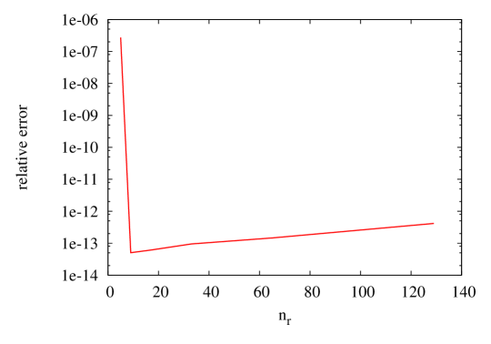
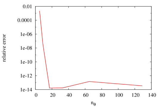
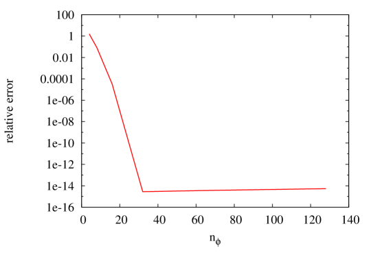
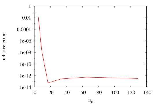
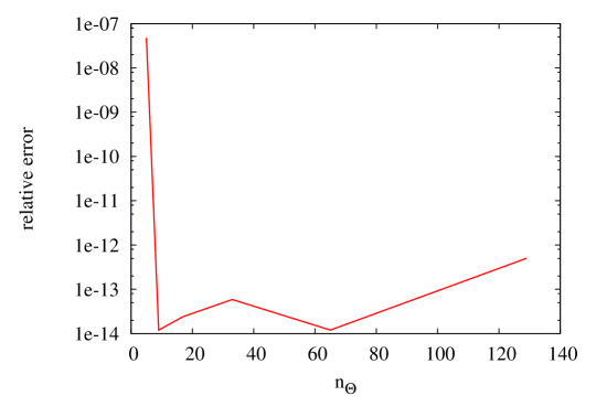
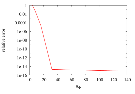
Figure 2: Relative error R.E., Eq. (48) as a function of the number of points in the tested dimension, for each of them ($r$, $\theta$, $\phi$, $\epsilon$, $\Theta$, $\Phi$). We can see a spectral (i.e., exponential) convergence in every case.

4.2 Collision term

The full collision operator is not yet implemented in our code. For the test cases we implement an isoenergetic scattering

$$B_{IS}=\frac{\epsilon^{2}}{(2\pi)^{3}}\int_{0}^{\pi}\int_{0}^{2\pi}R_{IS}\sin(\Theta^{\prime})\left[f(r,\theta,\phi,\epsilon,\Theta^{\prime},\Phi^{\prime})-f(r,\theta,\phi,\epsilon,\Theta,\Phi)\right]\mathrm{d}{}\Theta^{\prime}\mathrm{d}{}\Phi^{\prime},$$ (49)

with $R_{IS}$ the scattering kernel (see [44]). We choose to implement the scattering over nucleons (neutrons and protons), for which we follow [44]. This term is the only contribution to the collision operator implemented in the test cases.

An interesting point is that the collision term is often treated using a decomposition on Legendre polynomials, keeping only the first two terms (e.g. [44, 2]). Thus, it is possible to compare the spectral treatment using Legendre polynomials to our methods, knowing that in our case it is very easy to improve accuracy. This shall be done in a forthcoming study. There may not be very large differences between our method and the Legendre polynomial method, but in our opinion this is interesting to check.

4.3 Particle number conservation in GR

Here, for a given initial condition, we evolve the Boltzmann equation $L[f]=\mathcal{C}[f]$ in time and look whether the total number of neutrinos is conserved by our numerical scheme. The (time-dependent) number of particles is computed via

$$N(t)=\frac{1}{(2\pi)^{3}}\int f(t,r,\theta,\phi,\epsilon,\Theta,\Phi)\mathrm{d}^{6}V~{},$$ (50)

and the relative particle number conservation is computed as

$$\delta=\frac{N^{n}-N^{0}}{N^{0}}~{},$$ (51)

where $N^{n}$ is the number of particles at the $n$-th time step, and $N^{0}$ is the number of particles at the beginning of the simulation. $\delta$ is also corrected for the radial fluxes at the boundaries.

One radial shell is simulated, from $R_{\min}=1\ \textrm{km}$ to $R_{\max}=2.5\ \textrm{km}$. The boundary conditions are as follows: $f(R_{\min},\theta,\phi,\epsilon,\Theta<\pi/2,\Phi)$ is held constant (equal to the initial condition), and $f(R_{\max},\theta,\phi,\epsilon,\Theta>\pi/2,\Phi)=0$ and is also held constant. The time step is constant (see B.4 for an explanation of its calculation), and set to

$$\Delta t=0.1\frac{1}{n_{\Theta}^{2}}.$$ (52)

The initial conditions used are as follows,

$$f(r,\theta,\phi,\epsilon,\Theta,\Phi,t=0)=\left(\frac{p_{Z}}{\epsilon}\right)^{2}\times H\left(\Theta-\frac{\pi}{2}\right)~{},$$ (53)

where $H(\Theta-\pi/2)$ is the Heaviside function. $p_{Z}$ is the projection of the momentum vector on the corresponding Cartesian axis (see C for the detailed expression of this quantity).

In this test we evolve the Boltzmann equation Eq. (47) with the general relativistic Liouville operator, and use the collision operator that includes isoenergetic scattering where the value of the nucleon density $n_{b}=2\times 10^{13}\ \textrm{g.cm}^{-3}$ corresponds to an opaque regime . We do not make any assumptions about the symmetry of the system. We use $9\times 9\times 4\times 5\times 33\times 4$ points in $r\times\theta\times\phi\times\epsilon\times\Theta\times\Phi$.

To simplify matters we evolve our Boltzmann equation on a Schwarzschild spacetime background. The Schwarzschild metric is written in isotropic gauge

$$\mathrm{d}{}s^{2}=-\left(\frac{1-\frac{R_{s}}{4r}}{1+\frac{R_{s}}{4r}}\right)^{2}\mathrm{d}{}t^{2}+\left(1+\frac{R_{s}}{4r}\right)^{4}(\mathrm{d}{}r^{2}+r^{2}\mathrm{d}{}\theta^{2}+r^{2}\sin^{2}\theta\mathrm{d}{}\phi^{2}),$$ (54)

with $R_{s}=2M$ the Schwarzschild radius. This expression is nothing but the CFC expression of the line element in Eqs. (21) and (43), with

$$\alpha=\dfrac{1-\dfrac{R_{s}}{4r}}{1+\dfrac{R_{s}}{4r}},\quad\quad\beta^{i}=0\quad\textrm{and}\quad\Psi=1+\frac{R_{s}}{4r}.$$ (55)

In our simulations, we use $R_{s}=0.4\ \textrm{km}$ so that the horizon is not within the computational domain.

Figure 3: Particle conservation relative error as a function of time.

The particle number conservation is at most $\delta=10^{-4}$ all along the 50 simulated time steps (see Fig. 3). We checked that it is converging with decreasing the time step. This provides evidence that the time evolution is working and our calculation conserves the number of particles, with a small numerical error.

4.4 Gravitational redshift test

For this test, we again use the Schwarzschild metric and attempt to recover the expected gravitational redshift.

The physical setup of this test is described as follows. Consider a static observer at $r=R_{\rm min}$ that compares a neutrino spectrum he sees with the one of a static observer at $r=R_{\rm max}$.

The static observer is, by definition, the Eulerian observer. However, to compare the two spectra, we need to transform the observations into the CF, because it is the only global frame (recall that the EF at $R_{\rm min}$ is different from the EF at $R_{\rm max}$). In the EF, the 4-velocity is always $n^{\mu}=(1,0,0,0)$ and so a neutrino spectrum, as seen in the EF, would not experience any redshift.

In the CF, we have the usual formulation

$$\frac{\epsilon^{CF}_{2}}{\epsilon^{CF}_{1}}=\frac{\alpha_{1}}{\alpha_{2}},$$ (56)

where $1$ denotes the emission point and $2$ denotes the reception point. This equation can also be found by applying $M^{-1}$ to $n^{\mu}$.

The numerical test consists on simulating a radial shell with $R_{\rm min}=5M$ and $R_{\rm max}=12.5M$. We use a resolution $n_{r}=9$, $n_{\theta}=5$, $n_{\phi}=4$, $n_{\epsilon}=9$, $n_{\Theta}=5$, $n_{\Phi}=4$. With initial condition $f=0$ everywhere, except at the inner boundary ($r=R_{\rm min}$) where a flux of neutrinos is injected with a Gaussian profile in $\epsilon$. By solving the Boltzmann equation (without collisions, and without any assumption on symmetries), we recover the same Gaussian profile at $r=R_{\rm max}$ (see figure 4). We then transform the spectra to the CF to be able to compare them and to show the gravitational redshift.

Figure 4: Distribution function energy profiles in Schwarzschild spacetime (54), as seen by static observers. The profile at $r=R_{\rm min}$ (red, plain) is imposed, the profile at $r=R_{\rm max}$ (green, dashed) is then deduced after integration of the neutrino transport equation in vacuum. The observer 4-velocity has been transformed back to the CF for clarity.

As we see in figure 4, in the CF, the spectrum is redshifted when travelling from $R_{\rm min}$ to $R_{\rm max}$, by a factor $\alpha_{1}/\alpha_{2}=0.89$.

With this configuration (GR with no collision), a time step takes approximately one second. When improving the resolution to $n_{r}=17$, $n_{\theta}=9$, $n_{\phi}=4$, $n_{\epsilon}=17$, $n_{\Theta}=17$, $n_{\Phi}=4$, a time step takes approximately 23 seconds. Improving the resolution again by a factor of 2 with $n_{r}=17$, $n_{\theta}=9$, $n_{\phi}=4$, $n_{\epsilon}=17$, $n_{\Theta}=33$, $n_{\Phi}=4$, a time step take approximately 47 seconds. (tests done with a single processor Intel(R) Core(TM) i7-3630QM CPU with a frequency of 2.4 GHz).

4.5 Searchlight beam test

Figure 5: Searchlight beam test. The colors and the black contour lines code the value of the neutrino intensity, in an arbitrary $(r,\theta)$ plane. The spread of the beam is mostly due to the initial spread of the source, rather than numerical errors.

The searchlight beam test proposes to simulate the narrowest beam possible and look at the dispersion due to numerical errors [25, 45]. The dispersion must be reduced by increasing resolution.

With spectral methods, introducing a point source would result in considerable Gibbs phenomenon. When one tries to represent a non smooth (discontinuous) function with spectral methods, unwanted oscillations appear. This is called Gibbs phenomenon (see also B). The bigger the discontinuity, the bigger the oscillations, and if too big, the simulation may give wrong and unphysical results.

Instead of introducing a point source, we introduce a Gaussian shaped source, and try to get the narrowest Gaussian possible before have too much Gibbs phenomenon. Indeed, at a given resolution, the representation of narrower and narrower Gaussian leads to more and more Gibbs phenomenon, because a too narrow Gaussian approaches a discontinuous function.

Initial conditions for this test are as follow. One radial shell is simulated, from $R_{\min}=1\ \textrm{km}$ to $R_{\max}=2.5\ \textrm{km}$. We use a resolution $n_{r}=17$, $n_{\theta}=17$, $n_{\phi}=4$, $n_{\epsilon}=1$, $n_{\Theta}=17$, $n_{\Phi}=4$. We impose

$$f_{0}=\exp{-\frac{\left(r-\mu_{r}\right)^{2}}{2\sigma_{r}^{2}}}\times\exp{-\frac{\left(\theta-\mu_{\theta}\right)^{2}}{2\sigma_{\theta}^{2}}}\times\exp{-\frac{\left(\Theta-\mu_{\Theta}\right)^{2}}{2\sigma_{\Theta}^{2}}}~{},$$ (57)

with $\mu_{r}=1.2\ \textrm{km}$, $\mu_{\theta}=1.4$, $\mu_{\Theta}=0.1$, and $2\sigma_{r}^{2}=0.1\ \textrm{km}^{2}$, $2\sigma_{\theta}^{2}=2\sigma_{\Theta}^{2}=0.1$.

Because the chosen value for $\Theta$ is very close to $0$, $\Phi$ only plays a very minor role, so we do not multiply by a Gaussian in $\Phi$. Moreover, nothing depends on energy in this test, so we completely ignore the energy dependence ($n_{\epsilon}=1$). Finally, for simplicity we evolve the $\phi$ degree of freedom but we do not multiply by a Gaussian in $\phi$, so that the results can be plotted in 2D in a $r,\theta$ plane.

We evolve the Boltzmann equation without collision and without gravitation (as it would obscure the point), with the source continuously emitting neutrinos in the defined direction. We wait for the beam to cross the shell.

On figure 5, the result is shown in an arbitrary $(r,\theta)$ plane. The momentum space dependence has been integrated. The color codes the value of the distribution function (or, equivalently, the neutrino intensity, because energy is constant), and we also plot black contour lines. We see that the spreading is mostly due to the representation by Gaussian profiles of the source, more than numerical errors. So, by construction, increasing the resolution decreases the spread of the source. Finally, on figure 5, we see that profiles that narrow produce a small amount of unwanted Gibbs phenomenon. We note that this test would benefit from a comparison with a finite differences code, and we could give more quantitative results. We let this point for future work.

5 Conclusion

We have derived the general relativistic Boltzmann equation in doubly spherical coordinates and with the Liouville operator in the Eulerian frame, using a $3+1$ formalism. This derivation is particularly adapted for our purposes, as it does not contain any time derivative, typically hard to tackle with spectral methods. This formalism naturally avoids the singularity found in the different parts of the Boltzmann equation. We have presented a $3+1$ version of the Liouville operator, and then the conformally flat version. While we have worked in the CFC, the derivation presented here can easily be generalized to 2D/3D cases in full general relativity, in other gauge choices.

We have shown a first step towards numerically solving the general relativistic neutrino transport problem in core-collapse supernovae with spectral methods. The use of spectral methods, namely the decomposition using a Chebyshev basis for the $r$, $\Theta$, and $\epsilon$ coordinates, as well as the decomposition using a Fourier basis for the $\theta$, $\phi$, and $\Phi$ coordinates, leads to a substantial increase in numerical efficiency compared to existing finite difference methods which are the current standard tool used for the supernova neutrino problem. Ultimately, to reproduce the resolution of the finite difference solutions, we require up to five times fewer grid points per dimension. This fact allows us to solve the neutrino transport problem using a single processor on a desktop computer for the test cases, rather than super computers and a substantial amount of memory. This work is a significant step towards developing code that perform simulations of 3D supernova using 6D Boltzmann neutrino transport in a reasonable amount of time

A possible improvement would be to implement a conservative version of the Boltzmann equation (as discussed in [27, 32]). In these papers the authors demonstrate both the efficiency and the improved accuracy of the conservative version with respect to the non conservative version of the Boltzmann equation. The adaptation of the conservative version to spectral methods represents a substantial amount of work and remains to be done. The other direction of improvement is the treatment of the central region in spherical coordinates, which our code is not able to describe. This could be done with a coupling of our code with a flux-limited diffusion one, as we expect the center of the proto-neutron star to be opaque to the neutrinos during post-bounce phase in core-collapse simulations.

It would be fruitful to perform a direct comparison between the different methods used to approximate the Boltzmann equation. In this proposed study we could test the accuracy of different approximations, such as the momentum closure, the flux limited diffusion or the ray-by-ray approximation. However, it is not a straightforward task to link the use of moments in [18] to a given number of points in our treatment (points in our $\Theta$ dimension). This is primarily due to the fact that [18, 20] use a variable Eddington factor to close their system of equations. A comparison between this method and a full Boltzmann equation, in our opinion, would be a very valuable study. We discuss the collision operator in sparse detail, and in future work we will investigate in greater detail this operator. Particularly, it would be interesting to compare the accuracy of the treatment with two moments of a Legendre decomposition with our work.

Our work may be naturally extended by coupling it to a (magneto)hydrodynamic code such as CoCoNuT [46]. Before doing so, more work is needed to implement the velocity dependent terms.

Appendix A Ricci rotation coefficients: additional terms

From equation (42) we see that we need to calculate $d_{i0j}$ and $d_{ij0}$, or equivalently, $d^{i}\,\!_{0j}$ and $d^{i}\,\!_{j0}$. The algebraic steps needed to simplify these terms are presented in this appendix.

We first address the computation of the $d^{i}\,_{j0}$ components.

With the use of equation (33) we obtain

$$d^{i}\,\!_{j0}=-M^{-1}\,\!\!_{j}\,\!{}^{\tilde{\mu}}\,M^{-1}\,\!\!_{0}\,\!{}^{\tilde{\nu}}\,\frac{\partial M^{i}\,\!_{\tilde{\mu}}}{\partial x^{\tilde{\nu}}}.$$ (58)

Because $M^{-1}\,\!\!_{j}\,\!{}^{0}=0$ in our $3+1$ formulation, $\tilde{\mu}$ may be replaced by a spatial index, and thus

$$d^{i}\,\!_{j0}=-M^{-1}\,\!\!_{j}\,\!{}^{\tilde{k}}\,M^{-1}\,\!\!_{0}\,\!{}^{\tilde{\nu}}\,\frac{\partial M^{i}\,\!_{\tilde{k}}}{\partial x^{\tilde{\nu}}}.$$ (59)

Keeping in mind a $3+1$ approach we can then separate this into two terms: the first corresponds to $\tilde{\nu}=0$ with $M^{-1}\,\!\!_{0}\,\!{}^{0}=1/\alpha$ and the second to $\tilde{\nu}=\tilde{l}=1,2,3$ with $M^{-1}\,\!\!_{0}\,\!{}^{\tilde{l}}=-\beta^{\tilde{l}}/\alpha$,

$$d^{i}\,\!_{j0}=-\frac{1}{\alpha}M^{-1}\,\!\!_{j}\,\!{}^{\tilde{k}}\,\frac{\partial M^{i}\,\!_{\tilde{k}}}{\partial t}+M^{-1}\,\!\!_{j}\,\!{}^{\tilde{k}}\,\frac{\beta^{\tilde{l}}}{\alpha}\frac{\partial M^{i}\,\!_{\tilde{k}}}{\partial x^{\tilde{l}}}~{}.$$ (60)

With specialization to the CFC, the first term of Eq. (60) becomes

$$-\frac{1}{\alpha}M^{-1}\,\!\!_{j}\,\!{}^{\tilde{k}}\,\frac{\partial M^{i}\,\!_{\tilde{k}}}{\partial t}=-\frac{1}{\alpha}\frac{1}{\Psi^{2}}\frac{\partial\Psi^{2}}{\partial t}\delta_{j}\,\!^{i},$$ (61)

where $\delta_{j}\,\!^{i}$ is the Kronecker delta. Using the maximal slicing condition $K=K^{i}\,\!_{i}=0$, we have for the conformal factor

$$\frac{\partial\Psi}{\partial t}=\frac{\Psi}{6}\nabla_{k}\beta^{k},$$ (62)

(see [39]). We can then eliminate the explicit time derivative to get,

$$-\frac{1}{\alpha}M^{-1}\,\!\!_{j}\,\!{}^{\tilde{k}}\,\frac{\partial M^{i}\,\!_{\tilde{k}}}{\partial t}=-\frac{1}{3\alpha}\nabla_{k}\beta^{k}\delta_{j}\,\!^{i}.$$ (63)

Note that with another time slicing choice, or using another form for the spatial metric, this derivation would have to be adapted. However, in principle, it is still possible to get rid of the time derivative, following a similar procedure.

We now explicit the second term of Eq. (60). Within the CFC, the purely spatial parts of $M$ and $M^{-1}$ are diagonal, so the only non-zero spatial terms arise from $i=j=\tilde{k}$.

After some simplifications, we find:

$$M^{-1}\,\!\!_{1}\,\!{}^{\tilde{1}}\,\frac{\beta^{\tilde{l}}}{\alpha}\frac{\partial M^{1}\,\!_{\tilde{1}}}{\partial x^{\tilde{l}}} = \frac{1}{\alpha\Psi^{2}}\left[\beta^{r}\frac{\partial\Psi^{2}}{\partial r}+\beta^{\theta}\frac{\partial\Psi^{2}}{\partial\theta}+\beta^{\phi}\frac{\partial\Psi^{2}}{\partial\phi}\right],$$ (64)

$$M^{-1}\,\!\!_{2}\,\!{}^{\tilde{2}}\,\frac{\beta^{\tilde{l}}}{\alpha}\frac{\partial M^{2}\,\!_{\tilde{2}}}{\partial x^{\tilde{l}}} = \frac{1}{\alpha\Psi^{2}}\left[\frac{\beta^{r}}{r}\frac{\partial\Psi^{2}r}{\partial r}+\beta^{\theta}\frac{\partial\Psi^{2}}{\partial\theta}+\beta^{\phi}\frac{\partial\Psi^{2}}{\partial\phi}\right],$$ (65)

$$M^{-1}\,\!\!_{3}\,\!{}^{\tilde{3}}\,\frac{\beta^{\tilde{l}}}{\alpha}\frac{\partial M^{3}\,\!_{\tilde{3}}}{\partial x^{\tilde{l}}} = \frac{1}{\alpha\Psi^{2}}\left[\frac{\beta^{r}}{r}\frac{\partial\Psi^{2}r}{\partial r}+\frac{\beta^{\theta}}{\sin\theta}\frac{\partial\Psi^{2}\sin\theta}{\partial\theta}+\beta^{\phi}\frac{\partial\Psi^{2}}{\partial\phi}\right].$$ (66)

We now turn to the computation of the $d^{i}\,\!_{0j}$ term. From equation (33),

$$d^{i}\,\!_{0j}=-M^{-1}\,\!\!_{0}\,\!{}^{\tilde{\mu}}\,M^{-1}\,\!\!_{j}\,\!{}^{\tilde{\nu}}\,\frac{\partial M^{i}\,\!_{\tilde{\mu}}}{\partial x^{\tilde{\nu}}},$$ (67)

where we see that $d^{i}\,\!_{0j}$ is 0 if $\tilde{\nu}=0$ since $M^{-1}\,\!\!_{j}\,\!{}^{0}=0$. Hence the fact that $\tilde{\nu}$ can be replaced by a spatial index and $d^{i}\,\!_{0j}$ does not contain any time derivative. We also decompose $\tilde{\mu}$ in a $3+1$ fashion, with the temporal part and the spatial part,

$$d^{i}\,\!_{0j}=-M^{-1}\,\!\!_{0}\,\!{}^{0}\,M^{-1}\,\!\!_{j}\,\!{}^{\tilde{k}}\,\frac{\partial M^{i}\,\!_{0}}{\partial x^{\tilde{k}}}-M^{-1}\,\!\!_{0}\,\!{}^{\tilde{l}}\,M^{-1}\,\!\!_{j}\,\!{}^{\tilde{k}}\,\frac{\partial M^{i}\,\!_{\tilde{l}}}{\partial x^{\tilde{k}}}.$$ (68)

With $M^{-1}\,\!\!_{0}\,\!{}^{0}=1/\alpha$ and $M^{-1}\,\!\!_{0}\,\!{}^{\tilde{l}}=-\beta^{\tilde{l}}/\alpha$, we find

$$d^{i}\,\!_{0j}=-\frac{1}{\alpha}M^{-1}\,\!\!_{j}\,\!{}^{\tilde{k}}\,\frac{\partial M^{i}\,\!_{0}}{\partial x^{\tilde{k}}}+\frac{\beta^{\tilde{l}}}{\alpha}M^{-1}\,\!\!_{j}\,\!{}^{\tilde{k}}\,\frac{\partial M^{i}\,\!_{\tilde{l}}}{\partial x^{\tilde{k}}}.$$ (69)

Within the CFC, after some simplifications, the first term of Eq.(69) becomes

$$-\dfrac{1}{\alpha}M^{-1}\,\!\!_{j}\,\!{}^{\tilde{k}}\,\dfrac{\partial M^{i}\,\!_{0}}{\partial x^{\tilde{k}}}=-\dfrac{1}{\alpha\Psi^{2}}\begin{pmatrix}[2]\dfrac{\partial\Psi^{2}\beta^{r}}{\partial r}&\dfrac{\partial\Psi^{2}r\beta^{\theta}}{\partial r}&\sin\theta\dfrac{\partial\Psi^{2}r\beta^{\phi}}{\partial r}\\ \dfrac{1}{r}\dfrac{\partial\Psi^{2}\beta^{r}}{\partial\theta}&\dfrac{\partial\Psi^{2}\beta^{\theta}}{\partial\theta}&\dfrac{\partial\Psi^{2}\sin\theta\beta^{\phi}}{\partial\theta}\\ \dfrac{1}{r\sin\theta}\dfrac{\partial\Psi^{2}\beta^{r}}{\partial\phi}&\dfrac{1}{\sin\theta}\dfrac{\partial\Psi^{2}\beta^{\theta}}{\partial\phi}&\dfrac{\partial\Psi^{2}\beta^{\phi}}{\partial\phi}\\ \end{pmatrix}~{},$$ (70)

with $j$ the row index and $i$ the column index.

Within the CFC, after some simplifications, the second term of Eq.(69) becomes,

$$\dfrac{\beta^{\tilde{l}}}{\alpha}M^{-1}\,\!\!_{j}\,\!{}^{\tilde{k}}\,\dfrac{\partial M^{i}\,\!_{\tilde{l}}}{\partial x^{\tilde{k}}}=\dfrac{1}{\alpha\Psi^{2}}\begin{pmatrix}[2]\beta^{r}\dfrac{\partial\Psi^{2}}{\partial r}&\beta^{\theta}\dfrac{\partial\Psi^{2}r}{\partial r}&\beta^{\phi}\sin\theta\dfrac{\partial\Psi^{2}r}{\partial r}\\ \dfrac{\beta^{r}}{r}\dfrac{\partial\Psi^{2}}{\partial\theta}&\beta^{\theta}\dfrac{\partial\Psi^{2}}{\partial\theta}&\beta^{\phi}\dfrac{\partial\Psi^{2}\sin\theta}{\partial\theta}\\ \dfrac{\beta^{r}}{r\sin\theta}\dfrac{\partial\Psi^{2}}{\partial\phi}&\dfrac{\beta^{\theta}}{\sin\theta}\dfrac{\partial\Psi^{2}}{\partial\phi}&\beta^{\phi}\dfrac{\partial\Psi^{2}}{\partial\phi}\end{pmatrix}~{},$$ (71)

where, as before, $j$ is the row index and $i$ the column index.

Appendix B Implementation of the Boltzmann solver

We here give some technical details about Ghost for the numerical integration of the Boltzmann equation (47), which is based on the numerical library Lorene [47]. However, Ghost includes some generalization of our methods to the 6-dimensional case, as Lorene is bound to the 3-dimensional case. We first give some general concepts about spectral methods in one dimension, then the treatment of the 6-dimensional case is shown, then we detail the techniques for handling coordinate singularities appearing in the Liouville operator in doubly spherical coordinates, and finally we present the time integration scheme, together with the treatment of boundary conditions.

B.1 Spectral representation

In order to represent a function $f(x)$, the most straightforward method is to use a finite set of its values on a pre-defined grid. An alternative, that we use here, is to represent it through a finite set of coefficients of the decomposition of the function on a pre-defined spectral basis. The most straightforward example is the use of a truncated Fourier series for a periodic function:

$$f(x)\simeq\sum_{k=0}^{N}a_{k}\,\cos(kx)+\sum_{k=1}^{N}b_{k}\,\sin(kx),$$ (72)

where $f$ can be represented, up to some truncation error, by the set of $2N+1$ coefficients $\{a_{k},b_{k}\}$. It can be shown (see e.g. [48, 49]) that for smooth functions this truncation error decreases faster than any power of $N$. In practice, it is most often exponentially decreasing. If the function $f$ is only continuous and $k$-times differentiable, then the convergence of the truncation error goes as $1/N^{k+1}$. If $f$ is not periodic or discontinuous, then there is no convergence of the functional series (72) to $f$; this is called the Gibbs phenomenon [48].

When dealing with a non-periodic function, one can replace the Fourier basis by a set of orthogonal polynomials. The family of Jacobi polynomials [49] is well-suited for such representations with the particular cases of Legendre and Chebyshev polynomials. In our work, we use the Chebyshev polynomials to describe the non-periodic variables of our distribution function. In the case of a function $g(y)$ depending on the single variable $y\in[-1,1]$:

$$g(y)\simeq\sum_{k=0}^{N}c_{k}\,T_{k}(y),\textrm{ where }T_{k}(y)=\cos\left(k\arccos(y)\right)$$ (73)

is the $k$-th Chebyshev polynomial. Convergence rates of this series are the same as for Fourier series, depending on the degree of differentiability of $g(y)$. In B.2, we shall detail the implementation of the spectral representation of the distribution depending on six variables. We here first give the methods used in one dimension, using Fourier or Chebyshev decomposition basis, to compute derivatives or integrals.

If the Fourier coefficients of a periodic function $f(x)$ are known, it is rather simple to determine those of its derivative:

$$f^{\prime}(x)=\frac{\textrm{d}f}{\textrm{d}x}\simeq\sum_{k=1}^{N}\tilde{a}_{k}\,\cos(kx)+\tilde{b}_{k}\,\sin(kx),$$ (74)

where we can deduce the the $\{\tilde{a}_{k},\tilde{b}_{k}\}$ from the $\{a_{k},b_{k}\}$, through

$$\tilde{a}_{k}=k\,b_{k},\textrm{ and }\tilde{b}_{k}=-k\,a_{k}.$$ (75)

With Chebyshev polynomials, the coefficients $\tilde{c}_{k}$ of the derivative $g^{\prime}(y)$ are given by [49]:

$$\tilde{c}_{k}=\frac{2}{1+\delta_{0}^{\ k}}\sum_{\begin{subarray}{c}j=k+1\\ j+k\textrm{ odd}\end{subarray}}^{N}j\,c_{j}.$$ (76)

The computation of integral terms is done very easily with Fourier series: if the integral is taken over a period, one only needs to consider the coefficient $a_{0}$, the others terms giving zero. Integration of Chebyshev polynomials over the interval $[-1,1]$ gives:

$$\int_{-1}^{1}T_{k}(y)\,\textrm{d}y=\left\{\begin{array}[]{cl}-\dfrac{2}{k^{2}-1}&k\textrm{ even},\\ 0&k\textrm{ odd}.\end{array}\right.$$ (77)

Spectral coefficients $\{a_{k},b_{k}\}$ or $\{c_{k}\}$ can be computed via quadrature formula (see e.g. [49]), or using a Fast Fourier Transform (FFT). Indeed, from the definition of Chebyshev polynomials (73), it is possible to use a FFT to compute the coefficients $\{c_{k}\}$ [48]. Any of these methods require the knowledge of the values of function on a numerical grid: either equally spaced points for Fourier decomposition, or collocation points $\{x_{k}=-\cos\left(k\pi/N\right)\}$ for Chebyshev polynomials. Moreover, when non-linear terms are to be evaluated, as the product of two functions, the easiest way is to compute this product on the numerical grid, without using the coefficients (which would require the calculation of a convolution sum). Therefore, when representing a function $f(x)$ we will use a dual form with both descriptions: the values at grid points $\{f(x_{k})\}$ and the coefficients $\{a_{k},b_{k}\}$ or $\{c_{k}\}$, with the use of FFT to update each part, when needed. In what follows, we write the Fourier coefficients globally as

$$f(x)\simeq\sum_{k=0}^{n}c_{k}\,F_{k}(x)=\sum_{k=0}^{n/2}a_{k}\,\cos(kx)+\sum_{k=1}^{n/2}b_{k}\,\sin(kx).$$ (78)

B.2 Six-dimensional representation of the distribution function

At a given time-step $t$, the distribution function $f_{t}$ depends on six spatial variables in doubly spherical coordinates, and can be decomposed onto Chebyshev bases for the $r,\epsilon$ and $\Theta$ variables, whereas Fourier bases are used for $\theta,\phi$ and $\Phi$ variables. This can be written as follows:

$$f_{t}\left(r,\theta,\phi,\epsilon,\Theta,\Phi\right)\simeq\sum_{i=0}^{n_{r}}\sum_{j=0}^{n_{\theta}}\sum_{k=0}^{n_{\phi}}\sum_{l=0}^{n_{\epsilon}}\sum_{m=0}^{n_{\Theta}}\sum_{i=0}^{n_{\Phi}}C_{ijklmp}\,T_{i}(\bar{r})\,F_{j}(\theta)\,F_{k}(\phi)\,T_{l}(\bar{\epsilon})\,T_{m}(\bar{\Theta})\,F_{p}(\Phi).$$ (79)

The variables with a bar above belong to the interval $[-1,1]$ and are related to the coordinate variables through simple affine change, e.g.:

$$r=\alpha_{r}\bar{r}+\beta_{r},\qquad\bar{r}\in[-1,1],$$ (80)

where $(\alpha_{r},\beta_{r})$ are two constants, such that $R_{\rm min}=\beta_{r}-\alpha_{r}$ and $R_{\rm max}=\alpha_{r}+\beta_{r}$. A similar setting is chosen for the $\epsilon$ variable.

The nature of the Boltzmann equation explicitly requires a different treatment of boundary condition whether $\Theta\geq\pi/2$ or not. Indeed, $\Theta$ physically represents the direction (outgoing if $0\leq\Theta\leq\pi/2$ or ingoing if $\pi/2\leq\Theta\leq\pi$) of the neutrinos. For instance, the surface of an isolated proto-neutron star has an outgoing flux but no incoming flux, the distribution function is expected to be $\mathcal{C}^{0}$, but not differentiable, at $\Theta=\pi/2$ (see e.g. [17]). In a core-collapse context, the proto-neutron star is not isolated but can approach the described case enough to justify our special treatment of the $\Theta=\pi/2$ point. This is described in detail in [17]. As that path-finding study described, we also use the Chebyshev basis for the $\Theta$ argument, within the context of a multi-domain approach [50]. In particular, we split our $\Theta$ interval into two domains, separated at $\Theta=\pi/2$, as this allows us to benefit from the fast convergence of spectral methods despite the fact that the solution is only $\mathcal{C}^{0}$ continuous across this domain boundary. An affine change of variables of the type (80) is defined in each domain.

Particular care must be taken when dealing with the polar coordinate $\theta$. We have modified the existing methods in the Lorene library for this coordinate to allow for dependence on both the azimuthal ($\phi$) and momentum azimuthal ($\Phi$) coordinates. Based on regularity properties, the $\theta$ representation ($\sin{(j\theta)}$ or $\cos{(j\theta)}$) is deduced from the $\phi$ representation ($\sin{(m\phi)}$ or $\cos{(m\phi)}$) and the $\Phi$ representation ($\sin{(M\Phi)}$ or $\cos{(M\Phi)}$).

Let us, for a moment, consider a 3D scalar field $F(r,\theta,\phi)$. The representation of $F$ with Lorene has already been described e.g. in [29], and our treatment of a distribution function (a 6D scalar field) is a natural generalization of it. The technical point here is that the exact $\theta$ basis in Lorene is dependent on the nature of the $\phi$ and $\Phi$ bases, due to the singular character of spherical coordinates and to the regularity requirement on the axis $\theta=0$ of our functions (see [29] for details).

Typically, we expect that the decomposition (79) for functions $F(\theta,\phi)$ may be written as a linear combination of,

$$\sin{(j\theta)}\sin{(m\phi)},\,\sin{(j\theta)}\cos{(m\phi)},\,\cos{(j\theta)}\sin{(m\phi)},\,\cos{(j\theta)}\cos{(m\phi)}$$ (81)

The $\theta$ argument is decomposed on a basis with sines and cosines, depending on the parity of $m$, COSSIN_C or COSSIN_S which are defined as follows.

For regular scalar fields in 3D case, one needs the COSSIN_C basis, which is defined to be a series that uses the base elements

$$\left.\begin{array}[]{c}\cos{\left(j\theta\right)}\sin{(m\phi)}\\ \cos{\left(j\theta\right)}\cos{(m\phi)}\end{array}\right\}\rm{m\,even},$$ (82)

and

$$\left.\begin{array}[]{c}\sin{\left(j\theta\right)}\sin{(m\phi)}\\ \sin{\left(j\theta\right)}\cos{(m\phi)}\end{array}\right\}\rm{m\,odd},$$ (83)

In addition, the COSSIN_S basis uses,

$$\left.\begin{array}[]{c}\sin{\left(j\theta\right)}\sin{(m\phi)}\\ \sin{\left(j\theta\right)}\cos{(m\phi)}\end{array}\right\}\rm{m\,even},$$ (84)

and

$$\left.\begin{array}[]{c}\cos{\left(j\theta\right)}\sin{(m\phi)}\\ \cos{\left(j\theta\right)}\cos{(m\phi)}\end{array}\right\}\rm{m\,odd}.$$ (85)

So, COSSIN means an expansion in both cosines and sines for $\theta$, and _C (for cosine) or _S (for sine) refers to the expansion corresponding to $\cos{(0\,\phi)}$. It is straightforward to see that some operators, for instance $\partial/\partial\theta$, switch the basis from COSSIN_C to COSSIN_S and vice-versa. This is the reason why both bases are implemented.

Coming back to the six dimensional calculation, we consider expanding this definition to include the Fourier basis for the $\Phi$ argument. The base elements for a function $G(\theta,\phi,\Phi)$ are,

$$\begin{matrix}\sin{(j\theta)}\sin{(m\phi)}\sin{(M\Phi)},\quad\sin{(j\theta)}\sin{(m\phi)}\cos{(M\Phi)},\\ \cos{(j\theta)}\sin{(m\phi)}\sin{(M\Phi)},\quad\cos{(j\theta)}\sin{(m\phi)}\cos{(M\Phi)},\\ \sin{(j\theta)}\cos{(m\phi)}\sin{(M\Phi)},\quad\sin{(j\theta)}\cos{(m\phi)}\cos{(M\Phi)},\\ \cos{(j\theta)}\cos{(m\phi)}\sin{(M\Phi)},\quad\cos{(j\theta)}\cos{(m\phi)}\cos{(M\Phi)}.\end{matrix}$$ (86)

Analogously, the expansion rule can be inferred from the 3D treatment, but instead of considering the parity of $m$ alone, we consider the parity of the combination $m+M$. While this approach may appear to be complex, it allows us to manipulate a (regular) six dimensional scalar field in a fully consistent manner.

In the 6D case, for the decomposition of the distribution function, the new COSSIN_C basis corresponds to

$$\left.\begin{array}[]{c}\cos{\left(j\theta\right)}\cos{(m\phi)}\sin{(M\Phi)}\\ \cos{\left(j\theta\right)}\sin{(m\phi)}\sin{(M\Phi)}\\ \cos{\left(j\theta\right)}\cos{(m\phi)}\cos{(M\Phi)}\\ \cos{\left(j\theta\right)}\sin{(m\phi)}\cos{(M\Phi)}\end{array}\right\}\rm{(M+m)\,even},$$ (87)

and

$$\left.\begin{array}[]{c}\sin{\left(j\theta\right)}\cos{(m\phi)}\sin{(M\Phi)}\\ \sin{\left(j\theta\right)}\sin{(m\phi)}\sin{(M\Phi)}\\ \sin{\left(j\theta\right)}\cos{(m\phi)}\cos{(M\Phi)}\\ \sin{\left(j\theta\right)}\sin{(m\phi)}\cos{(M\Phi)}\end{array}\right\}\rm{(M+m)\,odd}$$ (88)

While the new COSSIN_S basis uses

$$\left.\begin{array}[]{c}\cos{\left(j\theta\right)}\cos{(m\phi)}\sin{(M\Phi)}\\ \cos{\left(j\theta\right)}\sin{(m\phi)}\sin{(M\Phi)}\\ \cos{\left(j\theta\right)}\cos{(m\phi)}\cos{(M\Phi)}\\ \cos{\left(j\theta\right)}\sin{(m\phi)}\cos{(M\Phi)}\end{array}\right\}\rm{(M+m)\,odd},$$ (89)

and

$$\left.\begin{array}[]{c}\sin{\left(j\theta\right)}\cos{(m\phi)}\sin{(M\Phi)}\\ \sin{\left(j\theta\right)}\sin{(m\phi)}\sin{(M\Phi)}\\ \sin{\left(j\theta\right)}\cos{(m\phi)}\cos{(M\Phi)}\\ \sin{\left(j\theta\right)}\sin{(m\phi)}\cos{(M\Phi)}\end{array}\right\}\rm{(M+m)\,even}.$$ (90)

B.3 Singularity-avoiding technique

There are two kinds of coordinate singularities which arise in our formulation. For instance, in Eq. (13) one can see that a coordinate singularity occurs at the origin where the radial coordinate $r$ goes to $0$, with the term $r^{-1}$ in front of all angular derivatives (in a similar way as in many other operators, like the Laplace operator). Another coordinate singularity occurs on the polar axis (with $\sin^{-1}(\theta)$ terms), again, akin to the Laplace operator this occurs on the terms with azimuthal and momentum-azimuthal derivatives in Eq. (13). Momentum-polar axis singularity (with $\sin^{-1}(\Theta)$ terms) appears in the relativistic Liouville operator, as can be seen in the expression of the Jacobian Eq. (2). Additional $\sin^{-1}(\theta)$ terms also occur in the Ricci rotation coefficients.

The singularity at the origin is not treated in this paper. The long term strategy is to use a simplified version in the innermost part, and to couple it to our full Boltzmann equation, that would take care of all other parts. The simplified version could be a diffusion equation or a telegraph equation (see [17] for a detailed discussion and implementation of the telegraph equation, as well as for the matching between both equations). This treatment is known to be sufficient in the innermost part of a core-collapse supernova simulation, and there are well known techniques to handle the singularity at the origin when using these approaches, described in [29]. In this work, we restrict ourselves to radial shells from a given $R_{\rm min}>0$ to a given $R_{\rm max}$.

The axial singularity is treated in the same fashion as in Lorene in 3D. Lorene’s operators are expressed using spherical geometry. If we take the Laplace operator as an example, we know that the full Laplace operator is regular, despite the individual terms being singular, if expressed in spherical coordinates. When combined, the apparent singularities parts analytically cancel and thus we do not need to compute them. Instead, singular operator as $\sin^{-1}(\theta)$ are computed only through their finite part (see also [29]). We exploit the same trends in our numerical development of the Liouville operator.

Practically speaking, when coding our solution we use the computed quantity $\bar{\Gamma}^{i}\,_{\mu\nu}\dfrac{\partial f}{\partial p^{i}}$. We first compute the partial derivative with respect to $p^{i}$, and then multiply by each term of the corresponding connection coefficient. The multiplication by the terms that may contain $\sin^{-1}(\theta)$ corresponds to the last step of the computation.

B.4 Time integration

With the tools described in B.1, B.2 and B.3 hereabove, it is possible to compute the spatial part of the relativistic Liouville operator, acting on a distribution function, as well as the collision term (49).

We note here $\tilde{L}$ the spatial part of the relativistic differential Liouville operator $L[f]$ (47):

$$\tilde{L}[f]=\alpha\left[\left(\frac{p^{i}}{\Psi^{2}\epsilon}-\frac{\beta^{i}}{\alpha}\right)\frac{\partial f}{\partial x^{i}}-\bar{\Gamma}^{j}\,\!_{\mu\nu}p^{\mu}p^{\nu}J^{i}\,\!_{j}\frac{1}{\epsilon}\frac{\partial f}{\partial p^{i}}\right].$$ (91)

The time integration of the relativistic Boltzmann equation for the distribution function $f(t,r,\theta,\phi,\epsilon,\Theta,\Phi)$, without the collision term can thus be written as

$$\frac{\partial f}{\partial t}=-\tilde{L}[f].$$ (92)

At every time $t$, the spectral approximation to the distribution function $f(t,\dots)$ is written as $U_{N}(t)$, the finite set of total size $N=n_{r}\times n_{\theta}\times n_{\phi}\times n_{\epsilon}\times n_{\Theta}\times n_{\Phi}$, composed of the time-dependent spectral coefficients $C_{ijklmp}$ of Eq. (79). We note $\tilde{L}_{N}$ the spectral approximation to the operator $\tilde{L}$, together with the boundary conditions which will be detailed hereafter. $\tilde{L}_{N}$ can be represented by an $N\times N$ matrix, although this matrix is never computed explicitly in our code. With this approach, we can use the so-called method of lines, which allows one to reduce a PDE to an ODE, after discretization in all but one dimensions. We can then, in principle, use any of the well-known ODE integration schemes (see e.g. [49]).

In Ghost we have, for the moment, implemented only equally-spaced grid in time, with the third-order Adams-Bashforth scheme:

$$U_{N}^{J+1}=U_{N}^{J}-\Delta t\left(\frac{23}{12}\tilde{L}_{N}U_{N}^{J}-\frac{4}{3}\tilde{L}_{N}U_{N}^{J-1}+\frac{5}{12}\tilde{L}_{N}U_{N}^{J-2}\right),$$ (93)

with $U_{N}^{J}=U_{N}(t=J\times\Delta t)$, $\Delta t$ being the time-step. This is an explicit scheme but, in principle, implicit or semi-implicit (see also [29]) schemes could be implemented. Thanks to the method of lines, usual stability analysis can be applied to any of the time-marching scheme, as $\tilde{L}_{N}$ can be diagonalized and it is possible to study the collection of scalar ODE problems:

$$\frac{\partial U_{N}}{\partial t}=\lambda_{i}U_{N},$$ (94)

where $\lambda_{i}$ is any of the eigenvalues of $\tilde{L}_{N}$. Standard result is that, of course, explicit schemes as the one we use here, are subject to the Courant-Friedrichs-Lewy (CFL) stability condition: the maximum time-step is of the order of magnitude of the time scale for propagation across the smallest distance between two grid points [48], [29]. From the definition of the grids we use in our code (see B.1 above), this distance goes as $1/n$ for the Fourier variables ($\theta,\phi,\Phi$) and $1/n^{2}$ for the Chebyshev ones ($r,\epsilon,\Theta$).

Boundary conditions are imposed using the tau method, which consists in modifying the last spectral coefficient, for each variable with a boundary condition, at each time-step. To illustrate this point, let us consider the simple advection PDE for an unknown function $v(t,x)$:

$$\forall t\geq 0,\forall x\in[-1,1],\quad \frac{\partial v}{\partial t}=\frac{\partial v}{\partial x}$$ (95)

$$\forall t\geq 0,\quad v(t,1)=b(t),$$

with $b(t)$ a given function. Let $V_{N}^{J}$ be the vector composed of the $N+1$ coefficients of $v(t=J\times\Delta t,x)$ in the Chebyshev basis. If we denote by $\ell_{N}$ the spectral approximation of the operator $\partial/\partial x$ and $\left(\ell_{N}V_{N}^{J}\right)_{i}$ the $i$-th coefficient of $\ell_{N}$ applied to $V_{N}^{J}$, then one can advance in time using the third-order Adams-Bashforth scheme:

$$V_{i}^{J+1}=V_{i}^{J}+\Delta t\left(\frac{23}{12}\ell_{N}V_{N}^{J}-\frac{4}{3}\ell_{N}V_{N}^{J-1}+\frac{5}{12}\ell_{N}V_{N}^{J-2}\right)_{i}\quad i=0\dots N-1,$$

$$V_{N}^{J+1}=b((J+1)\Delta t)-\sum_{k=0}^{N-1}V_{k}^{J+1}.$$ (96)

The expression on the last line comes from the fact that $T_{k}(x=1)=1$. Boundary conditions are thus imposed at $r=R_{\rm min}$ for $0\leq\Theta\leq\pi/2$ and $r=R_{\rm max}$ for $\pi/2\leq\Theta\leq\pi$, following [17].

Appendix C Doubly spherical coordinates transformation matrix $P$

In the $\vec{e}_{r},\vec{e}_{\theta},\vec{e}_{\phi}$ basis, $\vec{p}$ is defined by Eq.(1). We then apply two rotations of angles $\theta$ and $\phi$ to express $\vec{p}$ in the $\vec{e}_{x},\vec{e}_{y},\vec{e}_{z}$ basis (this is the usual transformation from a spherical to a Cartesian basis),

$$p_{x} = \epsilon(\cos\Theta\sin\theta\cos\phi+\sin\Theta\cos\Phi\cos\theta\cos\phi-\sin\Theta\sin\Phi\sin\phi)~{},$$

$$p_{y} = \epsilon(\cos\Theta\sin\theta\sin\phi+\sin\Theta\cos\Phi\cos\theta\sin\phi+\sin\Theta\sin\Phi\cos\phi)~{},$$

$$p_{z} = \epsilon(\cos\Theta\cos\theta-\sin\Theta\cos\Phi\sin\theta)~{}.$$ (97)

We then compute the transformation matrix $P_{1}$,

$$P_{1}=\dfrac{\partial(p_{x},p_{y},p_{z})}{\partial(\epsilon,\Theta,\Phi)}~{},$$ (98)

with

$$\frac{\partial p_{x}}{\partial\epsilon} = \frac{p_{x}}{\epsilon},\quad\quad\frac{\partial p_{y}}{\partial\epsilon}=\frac{p_{y}}{\epsilon},\quad\quad\frac{\partial p_{z}}{\partial\epsilon}=\frac{p_{z}}{\epsilon},$$

$$\frac{\partial p_{x}}{\partial\Theta} = \epsilon(-\sin\Theta\sin\theta\cos\phi+\cos\Theta\cos\Phi\cos\theta\cos\phi-\cos\Theta\sin\Phi\sin\phi),$$

$$\frac{\partial p_{y}}{\partial\Theta} = \epsilon(-\sin\Theta\sin\theta\sin\phi+\cos\Theta\cos\Phi\cos\theta\sin\phi+\cos\Theta\sin\Phi\cos\phi),$$

$$\frac{\partial p_{z}}{\partial\Theta} = \epsilon(-\sin\Theta\cos\theta-\cos\Theta\cos\Phi\sin\theta),$$

$$\frac{\partial p_{x}}{\partial\Phi} = \epsilon(-\sin\Theta\sin\Phi\cos\theta\cos\phi-\sin\Theta\cos\Phi\sin\phi),$$

$$\frac{\partial p_{y}}{\partial\Phi} = \epsilon(-\sin\Theta\sin\Phi\cos\theta\sin\phi+\sin\Theta\cos\Phi\cos\phi),$$

$$\frac{\partial p_{z}}{\partial\Phi} = \epsilon(\sin\Theta\sin\Phi\sin\theta).$$

We then compute the transformation matrix $P_{2}$,

$$P_{2}=\dfrac{\partial(p_{x},p_{y},p_{z})}{\partial(r,\theta,\phi)}~{},$$ (99)

with

$$\frac{\partial p_{x}}{\partial r} = 0,\quad\quad\frac{\partial p_{y}}{\partial r}=0,\quad\quad\frac{\partial p_{z}}{\partial r}=0,$$

$$\frac{\partial p_{x}}{\partial\theta} = \epsilon(\cos\Theta\cos\theta\cos\phi-\sin\Theta\cos\Phi\sin\theta\cos\phi),$$

$$\frac{\partial p_{y}}{\partial\theta} = \epsilon(\cos\Theta\cos\theta\sin\phi-\sin\Theta\cos\Phi\sin\theta\sin\phi),$$

$$\frac{\partial p_{z}}{\partial\theta} = \epsilon(-\cos\Theta\sin\theta-\sin\Theta\cos\Phi\cos\theta),$$

$$\frac{\partial p_{x}}{\partial\phi} = \epsilon(-\cos\Theta\sin\theta\sin\phi-\sin\Theta\cos\Phi\cos\theta\sin\phi-\sin\Theta\sin\Phi\cos\phi),$$

$$\frac{\partial p_{y}}{\partial\phi} = \epsilon(\cos\Theta\sin\theta\cos\phi+\sin\Theta\cos\Phi\cos\theta\cos\phi-\sin\Theta\sin\Phi\sin\phi),$$

$$\frac{\partial p_{z}}{\partial\phi} = 0.$$

The transformation matrix we need, $P$, is then

$$P=P_{1}^{-1}\times P_{2}~{},$$

$$P=\begin{pmatrix}[2]0,&0,&0,\\ 0,&\cos\Phi,&\sin\Phi\sin\theta,\\ 0,&-\dfrac{\sin\Phi\cos\Theta}{\sin\Theta},&\cos\theta+\sin\theta\dfrac{\cos\Phi\cos\Theta}{\sin\Theta},\end{pmatrix}~{},$$ (100)

which is the one used in section 2.2.

Bibliography

Bibliography

- [1] M. Liebendörfer, O. E. B. Messer, A. Mezzacappa, S. W. Bruenn, C. Y. Cardall, and F.-K. Thielemann. A Finite Difference Representation of Neutrino Radiation Hydrodynamics in Spherically Symmetric General Relativistic Spacetime. Astrophys. J. Suppl., 150:263–316, January 2004.
- [2] M. Rampp and H.-T. Janka. Radiation hydrodynamics with neutrinos. Variable Eddington factor method for core-collapse supernova simulations. Astron. Astrophys., 396:361–392, December 2002.
- [3] H.-T. Janka, F. Hanke, L. Hüdepohl, A. Marek, B. Müller, and M. Obergaulinger. Core-collapse supernovae: Reflections and directions. Prog. Theor. Exp. Phys., 2012(1):01A309, December 2012.
- [4] Y. Suwa, K. Kotake, T. Takiwaki, S. C. Whitehouse, M. Liebendörfer, and K. Sato. Explosion Geometry of a Rotating 13; Star Driven by the SASI-Aided Neutrino-Heating Supernova Mechanism. Proc. Astron. Soc. Jap., 62:L49, December 2010.
- [5] T. Takiwaki, K. Kotake, and Y. Suwa. Three-dimensional Hydrodynamic Core-collapse Supernova Simulations for an 11.2 Star with Spectral Neutrino Transport. Astrophys. J., 749:98, April 2012.
- [6] J. C. Dolence, A. Burrows, J. W. Murphy, and J. Nordhaus. Dimensional Dependence of the Hydrodynamics of Core-collapse Supernovae. Astrophys. J., 765:110, March 2013.
- [7] B. Müller, H.-T. Janka, and A. Marek. A New Multi-dimensional General Relativistic Neutrino Hydrodynamics Code for Core-collapse Supernovae. II. Relativistic Explosion Models of Core-collapse Supernovae. Astrophys. J., 756:84, September 2012.
- [8] K. Kotake, K. Sumiyoshi, S. Yamada, T. Takiwaki, T. Kuroda, Y. Suwa, and H. Nagakura. Core-Collapse Supernovae as Supercomputing Science: a status report toward 6D simulations with exact Boltzmann neutrino transport in full general relativity. Prog. Theor. Exp. Phys., 1:01A301, 2012.
- [9] E. J. Lentz, A. Mezzacappa, O. E. Bronson Messer, W. R. Hix, and S. W. Bruenn. Interplay of Neutrino Opacities in Core-collapse Supernova Simulations. Astrophys. J., 760:94, November 2012.
- [10] E. Abdikamalov, A. Burrows, C. D. Ott, F. Löffler, E. O’Connor, J. C. Dolence, and E. Schnetter. A New Monte Carlo Method for Time-dependent Neutrino Radiation Transport. Astrophys. J., 755:111, August 2012.
- [11] E. O’Connor and C. D. Ott. Black Hole Formation in Failing Core-Collapse Supernovae. Astrophys. J., 730:70, April 2011.
- [12] M. Ugliano, H.-T. Janka, A. Marek, and A. Arcones. Progenitor-Explosion Connection and Remnant Birth Masses for Neutrino-Driven Supernovae of Iron-Core Progenitors. Astrophys. J., 757:69, May 2012.
- [13] C. D. Ott, E. Abdikamalov, P. Moesta, R. Haas, S. Drasco, E. O’Connor, C. Reisswig, C. Meakin, and E. Schnetter. General-Relativistic Simulations of Three-Dimensional Core-Collapse Supernovae. Astrophys. J., 768:115, October 2013.
- [14] F. Hanke, A. Marek, B. Müller, and H.-T. Janka. Is Strong SASI Activity the Key to Successful Neutrino-driven Supernova Explosions? Astrophys. J., 755:138, August 2012.
- [15] J. Nordhaus, A. Burrows, A. Almgren, and J. Bell. Dimension as a Key to the Neutrino Mechanism of Core-collapse Supernova Explosions. Astrophys. J., 720:694–703, September 2010.
- [16] S. W. Bruenn, A. Mezzacappa, W. R. Hix, E. J. Lentz, O. E. Bronson Messer, E. J. Lingerfelt, J. M. Blondin, E. Endeve, P. Marronetti, and K. N. Yakunin. Axisymmetric Ab Initio Core-Collapse Supernova Simulations of 12-25 M_sol Stars. Astrophys. J. Lett., 767:L6, April 2013.
- [17] S. Bonazzola and N. Vasset. Solving the transport equation by the use of 6D spectral methods in spherical geometry. ArXiv e-prints, April 2011.
- [18] M. Shibata, K. Kiuchi, Y. Sekiguchi, and Y. Suwa. Truncated Moment Formalism for Radiation Hydrodynamics in Numerical Relativity. Prog. Theor. Phys., 125:1255–1287, June 2011.
- [19] M. Liebendörfer, S. C. Whitehouse, and T. Fischer. The Isotropic Diffusion Source Approximation for Supernova Neutrino Transport. Astrophys. J., 698:1174–1190, June 2009.
- [20] B. Müller, H.-T. Janka, and H. Dimmelmeier. A New Multi-dimensional General Relativistic Neutrino Hydrodynamic Code for Core-collapse Supernovae. I. Method and Code Tests in Spherical Symmetry. Astrophys. J. Suppl., 189:104–133, July 2010.
- [21] F. Hanke, B. Mueller, A. Wongwathanarat, A. Marek, and H.-T. Janka. SASI Activity in Three-Dimensional Neutrino-Hydrodynamics Simulations of Supernova Cores. Astrophys. J., 770:66, June 2013.
- [22] E. Livne, A. Burrows, R. Walder, I. Lichtenstadt, and T. A. Thompson. Two-dimensional, Time-dependent, Multigroup, Multiangle Radiation Hydrodynamics Test Simulation in the Core-Collapse Supernova Context. Astrophys. J., 609:277–287, July 2004.
- [23] C. D. Ott, A. Burrows, L. Dessart, and E. Livine. Two-dimensional multiangle, multigroup neutrino radiation-hydrodynamic simulations of postbounce supernova cores. Astrophys. J., 685:1069–1088, 2008.
- [24] E. J. Lentz, A. Mezzacappa, O. E. Bronson Messer, M. Liebendörfer, W. R. Hix, and S. W. Bruenn. On the Requirements for Realistic Modeling of Neutrino Transport in Simulations of Core-collapse Supernovae. Astrophys. J., 747:73, March 2012.
- [25] K. Sumiyoshi and S. Yamada. Neutrino Transfer in Three Dimensions for Core-collapse Supernovae. I. Static Configurations. Astrophys. J. Suppl., 199:17, March 2012.
- [26] D. Radice, E. Abdikamalov, L. Rezzolla, and C. D. Ott. A new spherical harmonics scheme for multi-dimensional radiation transport I. Static matter configurations. J. Comp. Phys., 242:648–669, June 2013.
- [27] C. Y. Cardall, E. Endeve, and A. Mezzacappa. Conservative 3+1 general relativistic variable Eddington tensor radiation transport equations. Phys. Rev. D, 87(10):103004, May 2013.
- [28] T. Kuroda, K. Kotake, and T. Takiwaki. Fully General Relativistic Simulations of Core-collapse Supernovae with an Approximate Neutrino Transport. Astrophys. J., 755:11, August 2012.
- [29] P. Grandclément and J. Novak. Spectral methods for numerical relativity. Living Rev. Relat., 12:1, 2009.
- [30] G. C. Pomraning. The equations of radiation hydrodynamics. Dover, 1973.
- [31] E. Gourgoulhon. 3+1 Formalism in General Relativity: Bases of Numerical Relativity, volume 846 of Lecture Notes in Physics. Springer, Berlin; New York, 2012.
- [32] E. Endeve, C. Y. Cardall, and A. Mezzacappa. Conservative Moment Equations for Neutrino Radiation Transport with Limited Relativity. ArXiv e-prints, December 2012.
- [33] J. M. Stewart. Non-equilibrium relativistic kinetic theory. In J. M. Stewart, editor, Non-equilibrium relativistic kinetic theory, volume 10 of Lecture Notes in Physics, Berlin Springer Verlag, pages 1–113, 1971.
- [34] C. Y. Cardall, E. J. Lentz, and A. Mezzacappa. Conservative special relativistic radiative transfer for multidimensional astrophysical simulations: Motivation and elaboration. Phys. Rev. D, 72(4):043007, August 2005.
- [35] F. Debbasch and W. A. van Leeuwen. General relativistic Boltzmann equation, I: Covariant treatment. Physica A Statistical Mechanics and its Applications, 388:1079–1104, April 2009.
- [36] F. Debbasch and W. A. van Leeuwen. General relativistic Boltzmann equation, II: Manifestly covariant treatment. Physica A Statistical Mechanics and its Applications, 388:1818–1834, May 2009.
- [37] R. W. Lindquist. Relativistic transport theory. Ann. Phys., 37:487–518, May 1966.
- [38] C. Y. Cardall, E. Endeve, and A. Mezzacappa. Conservative 3+1 General Relativistic Boltzmann Equation. ArXiv e-prints, April 2013. arXiv: 1305.0037.
- [39] I. Cordero-Carrión, P. Cerdá-Durán, H. Dimmelmeier, J.-L. Jaramillo, J. Novak, and E. Gourgoulhon. Improved constrained scheme for the Einstein equations : An approach to the uniqueness issue. Phys. Rev. D, 79(2):024017, 2009.
- [40] J. R. Wilson, G. J. Mathews, and P. Marronetti. Relativistic numerical model for close neutron-star binaries. Phys. Rev. D, 54:1317–1331, Jul 1996.
- [41] Masaru Shibata and Yuichiro Sekiguchi. Gravitational waves from axisymmetric rotating stellar core collapse to a neutron star in full general relativity. Phys. Rev. D, 69:084024, Apr 2004.
- [42] P. Cerdá-Durán, G. Faye, H. Dimmelmeier, J. A. Font, J. M. Ibáñez, E. Müller, and G. Schäfer. CFC+: improved dynamics and gravitational waveforms from relativistic core collapse simulations. Astron. Astrophys., 439:1033–1055, 2005.
- [43] A. Mezzacappa and R. A. Matzner. Computer simulation of time-dependent, spherically symmetric spacetimes containing radiating fluids - Formalism and code tests. Astrophys. J., 343:853–873, August 1989.
- [44] S. W. Bruenn. Stellar core collapse : numerical model and infall epoch. Astrophys. J. Suppl., 58:771–841, 1985.
- [45] J. M. Stone, D. Mihalas, and M. L. Norman. ZEUS-2D: A radiation magnetohydrodynamics code for astrophysical flows in two space dimensions. III - The radiation hydrodynamic algorithms and tests. Astrophys. J. Suppl., 80:819–845, June 1992.
- [46] H. Dimmelmeier, J. Novak, J. A. Font, J. M. Ibáñez, and E. Müller. Combining spectral and shock-capturing methods : A new numerical approach for 3d relativistic core collapse simulations. Phys. Rev. D, 71:064023, 2005.
- [47] E. Gourgoulhon, P. Grandclément, J.-A. Marck, and J. Novak. LORENE: Langage Objet pour la RElativité NumériquE. http://www.lorene.obspm.fr, 1997–2012.
- [48] J. B. Boyd. Chebyshev and Fourier Spectral Methods. Dover Publications, Mineola, New York, 2nd edition, 2001.
- [49] J. S. Hesthaven, S. Gottlieb, and D. Gottlieb. Spectral Methods for Time-Dependent Problems, volume 21 of Cambridge Monographs on Applied and Computational Mathematics. Cambridge University Press, Cambridge; New York, 2007.
- [50] C. Canuto, M. Y. Hussaini, A. Quarteroni, and T. A. Zang. Spectral Methods: Evolution to Complex Geometries and Applications to Fluid Dynamics. Scientific Computation. Springer, Berlin; New York, 2007.