Damping of radial electric field fluctuations in the TJ-II stellarator

Abstract

The drift kinetic equation is solved for low density TJ-II plasmas employing slowly varying, time-dependent profiles. This allows to simulate density ramp-up experiments and to describe from first principles the formation and physics of the radial electric field shear, which is associated to the transition from electron to ion root. We show that the range of frequencies of plasma potential fluctuations in which zonal flows are experimentally observed is neoclassically undamped in a neighborhood of the transition. This makes the electron root regime of stellarators, close to the transition to ion root, a propitious regime for the study of zonal-flow evolution. We present simulations of collisionless relaxation of zonal flows, in the sense of the Rosenbluth and Hinton test, that show an oscillatory behaviour in qualitative agreement with the experiment close to the transition.

1 Introduction

Sheared radial electric fields are generally accepted to play a central role in confinement transitions in fusion plasmas [1, 2, 3]. In non-quasisymmetric stellarators, the mean radial electric field is expected to be determined by the ambipolar condition of neoclassical fluxes [4, 5]. Nevertheless, turbulence-generated radial electric field fluctuations that display a zonal character have been observed in several stellarators [6, 7]. In this work, we discuss how turbulent momentum fluxes can overcome the collisional (due to neoclassical viscosity) and collisionless damping and modify the $E\times B$ rotation in the vicinity of a neoclassical bifurcation of the radial electric field [8].

The TJ-II stellarator exhibits such a bifurcation in low density plasmas with Electron Cyclotron Heating (ECH), see reference [9] and references therein. When a critical density $n_{cr}$ is reached, a spontaneous confinement transition takes place, associated with the formation of a shear layer. Experimentally, one of its most salient features is the emergence of zonal-flow-like electric potential structures [7, 10]. When the density decreases, the reverse transition occurs at a similar $n_{cr}$, but the amplitude of the zonal flows is smaller.

In this work, we solve the drift kinetic equation for slowly varying, time-dependent profiles. The evolution of the mean radial electric field is successfully described from first principles and we also provide a fundamental explanation for a wealth of experimental observations in the neighbourhood of the critical density. The key quantity is the neoclassical viscosity [11], which goes smoothly to zero when the critical density is approached from below. Since this viscosity acts as the restoring force of deviations of the radial electric field $E_{r}$ from ambipolarity, large $E_{r}$ excursions and, in particular, zonal flow fluctuations can be better observed. These predictions are illustrated in this work by density ramp experiments that exemplify the typical phenomena observed during the transition. The completion of the picture requires to study the time evolution of zonal flows in these plasmas. This is done by simulating the collisionless linear damping of zonal flows with the gyrokinetic code EUTERPE [12, 13]. These simulations are performed in a neoclassical background, and the predicted zonal flow oscillations are enhanced by the decrease of the radial electric field during the neoclassical bifurcation, in agreement with previous experimental observations.

The rest of the paper is organized as follows. Section 2 describes the experiments. Section 3 briefly introduces the equations and our definition of neoclassical viscosity that we will use to describe them; this is done in Section 4. Section 5 then looks more into detail the backward transition. Finally, Section 6 describes linear gyrokinetic simulations in the plasma conditions of our experiment. The conclusions are drawn in Section 7.

2 Experimental results

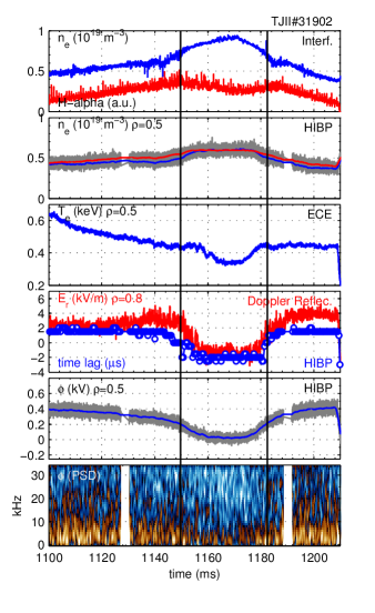
Figure 1: From top to bottom, temporal evolution, for discharge #31902, of the following quantities: $\overline{n_{e}}$ and $H_{\alpha}$ signal, $n_{e}(\rho=0.5)$, $T_{e}(\rho=0.5)$, $E_{r}(\rho=0.8)$ measured with Doppler Reflectometry and time-lag in the HIBP signal (proxy for the sign of $E_{r}(\rho=0.5)$, see text), $\phi(\rho=0.5)$, and spectrogram of the potential fluctuations at $\rho=0.5$.

In this section, we briefly describe experiments in which the main phenomenology associated to the low-density transition of TJ-II is present. These are the experimental results that we will try to reproduce in Sections 4 and  6 with simulations from first principles. Figure 1 shows the temporal traces of the relevant quantities in a representative discharge. The line-averaged density $\overline{n}_{e}$ is provided by interferometry. The local density and the plasma potential $\phi$ are measured by Heavy Ion Beam Probe (HIBP) at several radial positions ($\rho\!=\!0.5$ in the selected discharge, with $\rho\!=\!r/a$ the normalized radius, see below). The evolution of the local electron temperature $T_{e}$ is taken from Electron Cyclotron Emission (ECE). Both $T_{e}$ and $n_{e}$ are calibrated with Thomson Scattering (TS). The radial electric field $E_{r}$ at $\rho\!\approx\!0.8$ is taken from Doppler Reflectometry (DR).

The plasma density is increased at a constant rate by means of gas puffing and, for a constant ECH power input, $T_{e}$ decreases. When $\overline{n}_{e}$ reaches a value of about $0.6-0.7\times 10^{19}\,$m^-3 an spontaneous confinement transition takes place. The particle confinement time increases [14], as indicated by the $H_{\alpha}/n_{e}$ ratio, which drops (note also the change of slope in the $\overline{n}_{e}(t)$ curve). At the same time, $E_{r}$ changes from positive to negative. The local reversal of $E_{r}$ is observed by the DR; the reversal of $E_{r}$ at $\rho\!>\!0.5$ causes the drop in the plasma potential $\phi(\rho\!=\!0.5)$ measured by HIBP. Since $\phi(\rho\!=\!1)$ is set to 0 V, $\phi(\rho=0.5)$ contains information about $E_{r}(0.5\!<\!\rho\!<\!1.0)$, which makes it difficult to use this measurement to detect the local reversal of $E_{r}$. Instead, we use the time-lag in the detection of density fluctuations (which we assume advected by the $E\times B$ flow) in two poloidally-separated sample volumes of the HIBP, see figure 1. For discharges in which the position of measurement agree, we have checked that this procedure gives us information on the sign of $E_{r}$ in good agreement with DR.

We will see in the next section that the reversal of $E_{r}$ typically starts around the region where the density gradient is maximum, and a sheared $E_{r}$ appears which then propagates across the entire plasma radius at a speed of the order of several m/s [15] given by the density ramp. Then, further increase in $\overline{n}_{e}$ does not modify qualitatively $E_{r}$. In the selected discharge, the density ramp is relatively fast and this dynamics cannot be resolved: we see that $E_{r}$ changes sign almost simultaneously in all the region $\rho\!>\!0.5$.

Figure 1 also shows the evolution of the spectrum of low-frequency (tens of kHz) potential fluctuations measured by HIBP as the density ramp takes place. The amplitude of the fluctuations is smaller when $E_{r}$ is negative, and a maximum of fluctuations is detected for densities slightly lower than $n_{cr}$, although it is difficult to spot in figure 1. To show that these features are systematic, we plot in figure 2 (top) the average spectrum of the potential fluctuations at $\rho\!=\!0.5$ for two time windows, one corresponding to $n\!\lesssim\!n_{cr}$ and the other to $n\!>\!n_{cr}$, averaged over 17 reproducible discharges. The peak in fluctuations close below $n_{cr}$ is best seen in figure 2 (bottom), where we show the level of $E_{r}$ fluctuations ($\omega\!<200\,$kHz, with a large contribution of $\omega\!<50\,$kHz frequencies) measured by DR. for the same discharge of figure 1.

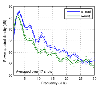
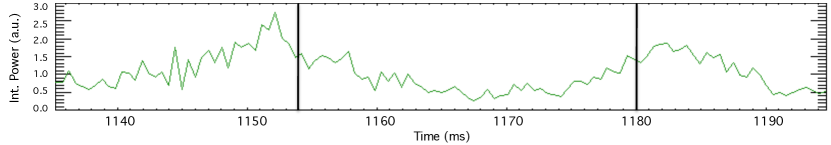
Figure 2: (top) Average spectrum of the potential fluctuations measured at $\rho\!=\!0.5$ by means of HIBP for $n\!\lesssim\!n_{cr}$ (electron root, blue) and $n\!>\!n_{cr}$ (ion root, green); (bottom) integrated power spectra measured by Doppler reflectometry at $\rho\!=\!0.8$ for the discharge of figure 1.

It is worth noting that in Refs. [16, 17] this peak of low-frequency potential fluctuations has been associated to Long Range Correlated (LRCed) electrostatic potential structures that grow when approaching the critical density and are a proxy to zonal flows.

Figures 1 and figure 2 also include the evolution of the plasma when the gas puffing rate is reduced and the density is ramped down. The particle confinement time goes back to pre-transition levels, $E_{r}$ goes back to positive and the potential fluctuations grow again. A peak in the level of fluctuations, of smaller amplitude, is observed after the transition, see figure 2 (bottom), consistently with previous observations [9]. No hysteresis in $E_{r}$ is evident from Figure 1, but a more detailed study will be made in Section 5.

3 Neoclassical equations and simulations

Most of the phenomenology described in the previous section will appear in this work as a natural consequence of a neoclassical bifurcation at $n_{cr}$. For this reason, we will briefly derive the equation for the evolution of the radial electric field that we will solve in the next sections. We start from the momentum balance equation [4] summed over species,

$$m_{i}\frac{\partial(n\mathbf{u})}{\partial t}+\nabla\cdot\Pi_{i}+\nabla\cdot\Pi_{e}=\mathbf{j}\times\mathbf{B}\,.~{}$$ (1)

Here, $\mathbf{u}$ is the ion flow tangent to flux surfaces, $\Pi_{s}$ is the viscosity tensor, $\Pi_{s}=m_{s}\int\mathbf{v}\mathbf{v}f_{s}(\mathbf{x},\mathbf{v},t)d^{3}\mathbf{v}$, or momentum flux of species $s$, $f_{s}$ its distribution function, and $\mathbf{j}\times\mathbf{B}$ is the Lorentz force. The projection of the latter over the flux-surface (proportional to the radial current), is set to zero unless otherwise stated. This is implied by quasineutrality ($\nabla\cdot\mathbf{j}=0$), but a net radial plasma current can be induced e.g. in plasma biasing experiments. We model a quasineutral plasma consisting of singly charged ions and electrons ($n_{e}\!=\!n_{i}\!=\!n$). Note that we have dropped the inertia of the electrons, given their much lower mass, $m_{e}/m_{i}\!\ll\!1$, but kept the electron viscosity tensor as it cannot be neglected in our low-$n$, high-$T_{e}$ ECH-heated plasmas [18]. We work in Hamada magnetic coordinates $(\psi,\theta,\xi)$, and follow the notation of reference [10]. The lowest order incompressible ion flow is conveniently written as

$$\mathbf{u}=2\pi\left(\frac{p_{i}^{\prime}(\psi)}{ne}+\phi^{\prime}(\psi)\right)\mathbf{e}_{\theta}+\Lambda(\psi)\mathbf{B}\,.$$ (2)

The flux surface label $\psi$ is the toroidal magnetic flux, $p_{i}$ is the ion pressure, $e$ is the elementary charge and the prime stands for differentiation with respect to the argument. The poloidal basis vector $\mathbf{e}_{\theta}\!=\partial\mathbf{r}/\partial\theta$ satisfies $\mathbf{e}_{\theta}\times\mathbf{B}=(2\pi)^{-1}\nabla\psi$, $\nabla\cdot\mathbf{e}_{\theta}=0$ and, for a currentless stellarator, $\langle{\mathbf{e}_{\theta}\cdot\mathbf{B}}\rangle=0$. We note that the form of the flow in equation (2) is derived under a transport ordering that reduces particle conservation to the incompressibility condition $\nabla\cdot\mathbf{u}=0$. The first term on the right-hand side of equation (2) contains the diamagnetic and $E\times B$ perpendicular flows, together with the parallel Pfirsch-Schlüter flow. The term $\Lambda\mathbf{B}$ is the ion bootstrap flow [19]. If we project equation (1) along $\mathbf{e}_{\theta}$ and take flux-surface-average, denoted by $\langle{\cdot}\rangle$, we obtain our evolution equation for the radial electric field,

$$\frac{\partial E_{r}}{\partial t} = \frac{1}{n}\frac{\partial}{\partial t}\left(\frac{p_{i}^{\prime}(r)}{e}\right)-E_{r}\frac{1}{n}\frac{\partial n}{\partial t}+$$ (3)

$$+ \frac{(\psi^{\prime}(r))^{2}}{4\pi^{2}{m_{i}}n\langle{\mathbf{e}_{\theta}\cdot\mathbf{e}_{\theta}}\rangle}\left(e(\Gamma_{e}-\Gamma_{i})+\langle{\mathbf{j}\cdot\nabla r}\rangle\right){.}$$

Here, $E_{r}\equiv-\phi^{\prime}(r)$ and the radius $r$ is a geometric flux label defined in terms of the volume $V(r)\!\equiv\!\pi r^{2}{L_{\textrm{\scriptsize ax}}}$, where ${L_{\textrm{\scriptsize ax}}}$ is the length of the magnetic axis and $V(a)$ is the total plasma volume, with $a$ the minor radius. We have obtained the radial particle fluxes from $\Gamma_{s}\!=\!-\frac{2\pi}{q_{s}\psi^{\prime}(r)}\langle{\mathbf{e}_{\theta}\cdot\nabla\cdot\Pi_{s}}\rangle$ [20]. The viscosity tensor can be split into a neoclassical part, given by the gyrotropic pressure tensor, and an anomalous contribution,

$$\Pi_{s}=\Pi_{s}^{NC}+\Pi_{s}^{an}=p_{s\|}\mathbf{b}\mathbf{b}+p_{s\perp}\left(\mathbf{I}-\mathbf{b}\mathbf{b}\right)+\Pi_{s}^{an}\,.$$ (4)

As mentioned above, in non-quasisymmetric confining magnetic topologies, the leading order contribution to equation (3) is $\langle{\mathbf{e}_{\theta}\cdot\nabla\cdot\Pi_{s}^{NC}}\rangle$, being much larger than $\langle{\mathbf{e}_{\theta}\cdot\nabla\cdot\Pi_{s}^{an}}\rangle$, which will be therefore neglected [4, 5].

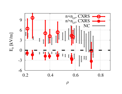
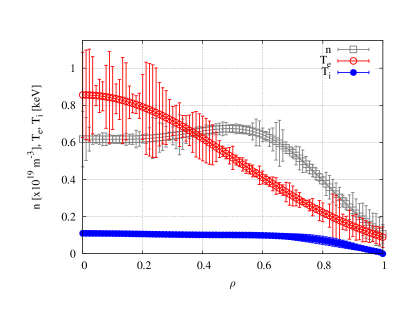
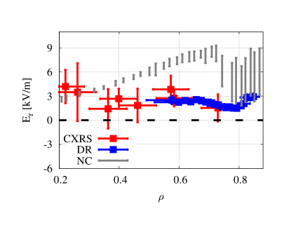
Figure 3: (top) Radial electric field profile measured by CXRS and compared to neoclassical calculations for $n\!<\!n_{cr}$ and $n\!>\!n_{cr}$; (center) plasma profiles of discharge #32599 , $n\!\lesssim\!n_{cr}$; (bottom) radial electric field profile measured by CXRS and DR compared to neoclassical calculations for a set of similar discharges that includes #32599.

We will use the Drift Kinetic Equation Solver (DKES) [21] complemented with momentum-conserving techniques [22] to evaluate the pressure anisotropy in a realistic TJ-II magnetic field equilibrium configuration in the parameter range in the vicinity of the transition. Details of the numerical calculation can be found in reference [18]. In order to check the accuracy of our numerical results, we first compare the predictions to Charge eXchange Recombination Spectroscopy (CXRS) measurements and Doppler Reflectometry of steady state $E_{r}$ in real discharges. We start from equation 3 and set to zero the time-dependent terms and the Lorentz force, i.e. we solve $E_{r}$ from the ambipolar equation for the radial neoclassical fluxes, $[\Gamma_{e}-\Gamma_{i}](E_{r})\!=0\,$.

Plasmas well below (above) $n_{cr}$ with $E_{r}$ positive (negative) in all plasma radius have been thoroughly studied in reference [23] and the predictions show good qualitative and quantitative agreement with CXRS measurements. For reference, we show some of the results in figure 3 (top). A similar exercise was performed already in reference [24], in which passive spectrometry measurements were in qualitative agreement with neoclassical calculations.

Nevertheless, as we will see later when studying the ambipolar equation of these plasmas, the closer one gets to $n_{cr}$, the more challenging it is to calculate the precise value of $E_{r}$. This can already be seen in figure 1 where, close to $n_{cr}$, $E_{r}$ varies much faster than $n_{e}$ or $T_{e}$. This will set a limit to the accuracy of our quantitative predictions. Both measurements and predictions include results from a set of 5 reproducible discharges, one of which is shown in figure 3 (center), and the results of our comparison are presented in figure 3 (bottom). According to the measurements, $E_{r}$ is positive in all the plasma radius. At $\rho\!\approx\!0.8$, the DR measures a minimum of $E_{r}$, with a double-shear layer at both sides of it. It is precisely at this radial position where the reversal of $E_{r}$ typically starts [15] which means that indeed the plasma is very close to the transition.

The predicted neoclassical $E_{r}$ is positive, in agreement with the experiment. We observe the double-shear-layer forming although at a slightly outer radial position. Finally, our calculations overestimate $E_{r}$ in the region $0.5\!<\rho\!<\!0.8$. The results are consistent with an underestimation of the ion radial flux: our calculation is radially local; if finite-orbit-width effects were included in the calculation of the ion radial flux [25], the theoretical predictions would probably come closer to the experiment. This is currently under investigation.

It is now clear that, although we probably will overestimate $n_{cr}$, our ordering assumption is valid for capturing the behaviour of $E_{r}$ during the low density transition: the leading term in the radial current is neoclassical and sets the value of $E_{r}$; turbulent contributions will be present and will produce excursions of $E_{r}$ from its ambipolar value, see figure 1 (bottom) and 2. Let us now show that these fluctuations can also, to some extent, be discussed in terms of equation (3). First, we expand the radial neoclassical current around the ambipolar radial electric field $E_{r}^{0}$,

$$[\Gamma_{e}-\Gamma_{i}](E_{r})\!=-\mu_{p}(E_{r}-E_{r}^{0})+O((E_{r}-E_{r}^{0})^{2}).$$ (5)

The neoclassical viscosity, $\mu_{p}$, is defined as the linear coefficient in this expansion. If we neglect the slow variations in $n$ and $T_{e}$, equation (3) yields

$$\frac{\partial\delta E_{r}}{\partial t} \approx\frac{e(\psi^{\prime}(r))^{2}}{4\pi^{2}mn\langle{\mathbf{e}_{\theta}\cdot\mathbf{e}_{\theta}}\rangle}\Bigg{[}\mu_{p}\delta E_{r}-\frac{\langle{\mathbf{j}\cdot\nabla r}\rangle}{e}\Bigg{]}$$ (6)

$$=-\nu_{p}\delta E_{r}+\check{j_{r}},$$

where $\delta E_{r}=E_{r}-E_{r}^{0}$, and constants have been absorbed in $\check{j_{r}}$ and in the viscosity $\nu_{p}$, which now has dimensions of frequency. Equation 6 is then meant to model the evolution of dynamically incompressible $E\times B$ flow fluctuations, $\tilde{\mathbf{u}}=-(2\pi/\psi^{\prime}(r))\delta E_{r}\mathbf{e}_{\theta}$, with the perpendicular flow $\tilde{\mathbf{u}}_{\perp}=\delta E_{r}\nabla r\times\mathbf{B}/B^{2}=-(2\pi/\psi^{\prime}(r))\delta E_{r}{\mathbf{e}_{\theta}}_{\perp}$ instantly accompanied by a parallel Pfirsch-Schlüter flow $\tilde{\mathbf{u}}_{\|}=-(2\pi/\psi^{\prime}(r))\delta E_{r}{\mathbf{e}_{\theta}}_{\|}$. This results in the inertia factor $\langle{\mathbf{e}_{\theta}\cdot\mathbf{e}_{\theta}}\rangle\approx r^{2}(1+2/\iota^{2})$, with the $2/\iota^{2}$ term coming from the parallel flow response [26]. Typical rotational transform values in the edge of TJ-II are $\iota(a)\sim 1.5$ which do not substantially modify $\nu_{p}$ values. The assumption of dynamically incompressible $E\times B$ flow fluctuations is justified for fluctuation frequencies below the acoustic characteristic frequency of GAM oscillations. As shown in Section 6, this frequency is about $40$ kHz for the TJ-II plasmas under study, to be compared with typical zonal flow frequencies $\lesssim 10$kHz [17, 10].

In reference [11] $\check{j_{r}}$ represented the radial current driven by an electrode, and the behaviour of $E_{r}$ during biasing experiments [27, 17] was successfully reproduced. In this work, we will use it to understand the behaviour of $E_{r}$ fluctuations during the density scan: $\check{j_{r}}$ will be the driving term of fluctuations (e.g. Reynolds Stress) and $\nu_{p}$ a restoring force towards neoclassical ambipolarity. To make the argument more precise, we Fourier transform equation (6) and multiply times the complex-conjugate for time scales faster than that of the density ramp, i.e., $\omega\!>\!\partial_{t}\log(E_{r}^{0})\!\sim\!\partial_{t}\log(n)\!\sim\!10\,$Hz, and obtain

$$|\hat{\delta E_{r}}(\omega)|^{2}=\frac{1}{\nu_{p}^{2}+\omega^{2}}|\hat{j}(\omega)|^{2}\,.$$ (7)

Equation 7 shows that the amplitude of the fluctuations $\hat{\delta E_{r}}(\omega)$ driven by a given broadband turbulent forcing $\hat{j}(\omega)$ is modulated by the neoclassical viscosity, which damps fluctuations of frequencies lower than $\nu_{p}$. We will see in the next section that, for our plasma conditions, $\nu_{p}\!\sim\!1-10$ kHz, of the order of the relevant frequencies in figure 2.

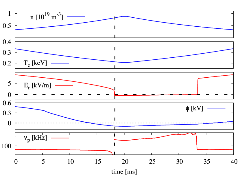
Figure 4: From top to bottom, temporal evolution during the numerical ramp of the following quantities at $\rho\!=\!0.7$ : $n_{e}$, $T_{e}$, $E_{r}$, $\phi$ , and $\nu_{p}$.

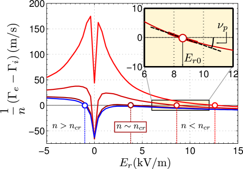
Figure 5: Ambipolar equation at $\rho\!=\!0.7$ for several representative times; (inset) sketch of the estimation of the viscosity.

4 Neoclassical description of the low-density transition

We now perform a dynamical neoclassical calculation of the formation of the sheared $E_{r}$. We therefore use equation (3) and try to simulate the density ramp-up and ramp-down of figure 1. We take smoothed plasma profiles similar to those of figure 3 (top) and make them evolve according to

$$\frac{1}{n}\frac{\mathrm{d}n}{\mathrm{d}t}={\pm 50\,\mathrm{s}^{-1}}\,,\quad\frac{1}{T_{e}}\frac{\mathrm{d}T_{e}}{\mathrm{d}t}={\mp 25\,\mathrm{s}^{-1}}\,,\quad\frac{\mathrm{d}T_{i}}{\mathrm{d}t}=0\,,$$ (8)

where the signs depend on the stage of the ramp. Note that a simulation of the evolution of $n(\rho,t)$, $T_{e}(\rho,t)$ and $T_{i}(\rho,t)$ is not required for the description of the formation of the $E_{r}$-shear of TJ-II; the existence of anomalous fluxes and sources is implicitly accounted for in the choice of $n(\rho,t)$, $T_{e}(\rho,t)$ and $T_{i}(\rho,t)$.

For low (high) density, the predicted neoclassical $E_{r}$ is positive (negative) in all the plasma radius, as in figure 3 and reference [23]. The evolution of the $E_{r}$ profile between these two situations (i.e., formation and evolution of the $E_{r}$-shear) was discussed in reference [11]. Since our calculation is radially local, we focus here in one representative radial position, $\rho\!=\!0.7$.

The result of the numerical density scan at this position is presented in figure 4, which is to be compared to figure 1. As $n$ rises and $T_{e}$ decreases, $E_{r}$ becomes less positive. Then, for $n_{e}\!\approx\!0.7\times 10^{19}\,$m${}^{-3}\,$ and $T_{e}\!\approx\!200\,$eV, there is a change of root: $E_{r}$ goes from positive to negative in a time-scale of several tens of $\mu$s. Further increase in $n$ then causes $E_{r}$ to be more negative. The plasma potential $\phi$ evolves according to $E_{r}$, and therefore decreases during the transition.

In figure 4 (bottom) we also plot the time evolution of the neoclassical viscosity $\nu_{p}$. When the plasma is in the ion root, the viscosity is much larger and, according to equation (7), the fluctuations have much smaller amplitude, as in figure 1. Immediately before the transition, a peak of the low-frequency $E_{r}$ fluctuations is predicted because of the vanishing $\nu_{p}$, which we discuss below.

We observe exactly the opposite behaviour ($E_{r}$ becomes less negative and more positive, $\phi$ evolves accordingly, and the level of fluctuations grows again) during the density ramp-down. The only difference is the predicted values of $n_{cr}$ for the backward transition, which differs from that of the forward transition. No vanishing of $\nu_{p}$ is predicted. These issues will be further discussed in Section 5.

Since the characteristic time scale of evolution of $E_{r}$ (10^-5 s) is much faster than that of the plasma profiles (10^-2 s), it is meaningful to discuss the results of figure 4 in the light of the ambipolar equation of the neoclassical radial fluxes for several selected plasmas of our density scan. In figure 5, we show the radial neoclassical current as a function of $E_{r}$ at $\rho\!=\!0.7$ for several relevant instants of the density ramp. This figure is characteristic of the low-collisionality regime of stellarators [8]. For very low collisionalities ($n\!\ll\!n_{cr}$) the only solution is a positive $E_{r}$ (electron root); for higher collisionalities ($n\!\gg\!n_{cr}$) the only solution is a negative $E_{r}$ (ion root). In these two situations, an increase in collisionality leads to less positive or more negative $E_{r}$. In the electron root regime, the variation of $E_{r}$ is larger, due to the smaller slope of the curve $[\Gamma_{e}-\Gamma_{i}](E_{r})$. For intermediate collisionalities, three solutions of the ambipolar equation, one of them unstable, coexist. We will define the critical density $n_{cr}$ (respectively, the critical temperature $T_{cr}$) as the local density (respectively, the local electron temperature) at which one of the two stable roots disappears, so that $E_{r}$ ‘jumps’ to the other solution. We discuss about this criterion in Section 5.

The qualitative behaviour of the viscosity can be extracted from the slope of the curves in figure 5 (inset). It is larger in the ion root regime than in the electron root, thus allowing for smaller fluctuations $\delta E_{r}$ provided that the forcing $\check{j_{r}}$ does not change. According to figure 4 (bottom) $\nu_{p}$ takes values of a few tens of kHz in the electron root regime and around 100 kHz in ion root. Following equation (7), fluctuations of frequencies of about 10 kHz will be more damped in the ion root. For higher-frequency harmonics, equation (7) becomes $|\hat{\delta E_{r}}|/|\hat{j_{r}}|\!\sim\!\omega^{-1}$ and no differences are expected between the two regimes. These predictions are in qualitative agreement with figure 2 (top). Figure 2 (bottom) shows that at the density for which the electron root disappears the viscosity vanishes, allowing for even larger fluctuations $\delta E_{r}$. Note that as the transition approaches and $\nu_{p}$ decreases, higher-order terms in the viscosity tensor of equation (4) (including those that depend on the $E_{r}$ shear) start to count in the evolution of $E_{r}$. Anyway, the experimental results of figures 1 and 2 prove that the reduction of $\nu_{p}$, that we predict without including such higher-order terms, is a significant physical phenomenon with measurable effects on the behaviour of $E_{r}$.

A similar discussion was made with a simplified neoclassical formulation in reference [28], where the zonal-flow neoclassical damping was predicted to be smaller in electron root regimes, which was speculated to explain the enhanced confinement in core-electron root plasmas of some stellarators. A full understanding of this phenomenon would require an appropriate calculation of $\check{j_{r}}$ and also to include non-local terms in the drift-kinetic equation in order to study the damping of zonal flows. Some calculations in this direction are presented in Section 6. In the present section, within the neoclassical framework, we predict a peaking of the low-frequency $E_{r}$ fluctuations in the electron root of stellarators, at the critical density, and we present direct experimental evidence. We also note that the involved frequencies are the ones expected to display higher LRCs, since they are roughly below the electron transit frequency for these plasmas. Therefore the vanishing of the neoclassical viscosity provides a fundamental explanation of why LRCs, and hence zonal flows, are preferentially observed close before the low-density transition of TJ-II.

Interestingly, LRCs are also observed close before the L-H transition of TJ-II. According to figure 5, if one further increases the density beyond the regime of the experiments in this work, the slope of the ambipolar equation decreases and the low-frequency fluctuations in $E_{r}$ are expected to increase again. Nevertheless, for those plasmas the ambipolar equation is always similar to the one for $n\!>\!n_{cr}$ in figure 5, according to our calculations: no change of root and therefore no vanishing of $\nu_{p}$ is predicted.

When the density is reduced, the radial electric field goes back to positive at a different critical density. No vanishing of the viscosity is predicted in the backward transition from ion to electron root, and no peaking of low frequency $E_{r}$ oscillations. Nevertheless, these results should be taken with caution due to some uncertainties in our calculation of the backward transition that we discuss in Section 5.

The low density transition has been observed for a large set of TJ-II magnetic configurations, with quantitative but no qualitative differences in the evolution of $E_{r}$ [29]. No dependence was found on $\iota$ (and therefore on the presence of low-order rational surfaces in the plasma), and larger configurations underwent the transition for smaller $\overline{n}_{e}$. This is consistent with a neoclassical discussion of the transition: in this low collisionality regime, the radial neoclassical fluxes do not depend on the rotational transform and depend strongly on the volume (roughly speaking, the magnetic field strenght modulation in a surface labelled by the normalized radius $\rho$ is larger for larger volumes). We have repeated the calculations for several configurations usually operated in TJ-II, and observed qualitative agreement with the experiment. Along the same line of reasoning, no qualitative differences between configurations are expected in the behaviour of the neoclassical viscosity either. At the critical density, it will vanish; far from it, since large configurations will have larger $\Gamma_{i}(E_{r})$ and $\Gamma_{e}(E_{r})$, equation (6) predicts smaller low-frequency $E_{r}$ fluctuations for them, assuming that every other parameter in the plasma is kept the same.

5 The backward transition

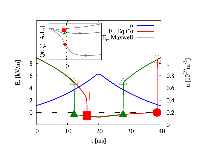
Figure 6: Evolution of $E_{r}$ during the numerical density ramp for the two criteria of change of root; (inset) heat production rate for several instants of the ramp

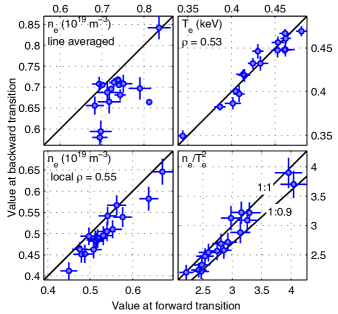
Figure 7: Value at the backward transition versus value at the forward transition of: $\overline{n}_{e}$ (top-left), local $n_{e}$ (bottom-left), local $T_{e}$ (top-right), and local $n_{e}/T_{e}^{2}$ (bottom-right).

Figure 4 describes the evolution of $E_{r}$ and the neoclassical fluxes when the density is reduced. A very salient feature is that a large hysteresis in $E_{r}$ is predicted which is not seen in figure 1. It should be noted that this is, at least partly, an artificial consequence of our choice of numerical scheme. This requires a brief discussion.

In the previous section, we stated that we consider that the transition takes place when the root in which the system is ceases to exist. Nevertheless, from a thermodynamic point of view, one should note that in the real system there are fluctuations and, if these are large enough, they will make the system “jump” from one stable root to the other before the first one disappears. A heuristic thermodynamical criterion is usually employed in these kind of calculations (see reference [30] and references therein): it is considered that the value of $E_{r}$ should be the one that minimizes the heat production rate defined as

$$Q(E_{r})\equiv\int^{E_{r}}[\Gamma_{e}-\Gamma_{i}](E_{r}^{\prime})\mathrm{d}E_{r}^{\prime}\,.$$ (9)

It is easy to see that the minima of $Q(E_{r})$ correspond to the stable solutions of the ambipolar equation. When the latter has only one root, both criteria yield the same result. When there are two stable solutions, $Q(E_{r})$ has two minima. According to Eq 3, the transition takes place when the minimum at which the system is disappears (open squares and closed circles in figure 6); according to the thermodynamical argument (called ‘Maxwell construction’) it takes place when this minimum ceases to be the absolute minimum of $Q$ (triangles in figure 6).

Figure 6 shows that our procedure of Section 4 slightly overestimates $n_{cr}$ for the forward transition as compared with the Maxwell construction (but it is still close to the experimental result). Note that an accurate estimate of $n_{cr}$ with the Maxwell criterium requires a very precise calculation of the neoclassical fluxes close to $E_{r}\!=\!0$, which is not possible with DKES, and demands much more computing time. On the other hand, our procedure largely underestimates $n_{cr}$ at the backward transition, and a large (and rather unrealistic) hysteresis is predicted by our procedure and not by the Maxwell constraint.

Since the latter is a heuristic criterium, it is meaningful to look more carefully at the experimental data behind figure 1 and a set of similar discharges and see if some of this hysteresis is indeed present. In order words, to check experimentally whether one of these criteria describes perfectly the experiment or if the behaviour of the real system lies somewhere in between the two predictions. In figure 7 we show, for all the discharges of this work with measurements at $\rho\!=\!0.55$, the value of the relevant quantities at the backward transition versus their value at the forward transition. The transition time is estimated from the time-lag in the HIBP signals, as in figure 1. The backward transition systematically takes place at lower line-densities. Nevertheless, since change of root is a radially local feature, we focus the search of hysteresis in the local densities, temperature and electron collisionality (which, due to the uncertainty in the $T_{i}$ measurement, we take simply proportional to $n_{e}/T_{e}^{2}$). The backward transition takes place at local density around 5% smaller and roughly at the same local $T_{e}$ (and hence at a collisionality 5% smaller). This hysteresis is of the same sign as our calculation in figure 4 although much smaller.

It should be noted that, in our calculations, the plasma profiles ($n$, $T_{e}$ and $T_{i}$) for a given $\overline{n}_{e}$ are exactly the same during the density ramp-up and ramp-down. This is not guaranteed in the experiment, where we cannot measure all the thermodynamical forces $n^{\prime}/n$, $T_{s}^{\prime}/T_{s}$ and $q_{s}E_{r}/T_{s}$ at the required times. A careful study was made in Refs. [15, 9] for the density, and it was concluded that $n^{\prime}/n$ was very similar at the two crossings of $n_{cr}$. Since we are in a regime where $E_{r}$ is mainly determined by the strong dependence of $\Gamma_{e}$ on the collisionality, it is reasonable to assume that the differences in the thermodynamical forces will be small enough not to play a relevant role. This working hypothesis is supported by analyses equivalent to that of figure 7 made (with less statistics) for more external radial positions in which similar results are observed.

Finally, it is worth noting that, according to the Maxwell construction, the forward transition takes place slightly before the electron root disappears (open triangle in figure 6), and therefore the neoclassical viscosity will reduce but not vanish (note that even if it vanished, there would be second-order contributions to equation (5) that would keep the fluctuations finite). Conversely, the backwards transition will lead the plasma to this same regime of reduced viscosity (open triangle instead of open circle), which would explain the second peak in Fig 2 bottom. The fact that the second peak has usually smaller amplitude is another experimental indication of the existence of some hysteresis.

6 Gyrokinetic simulations of zonal flow relaxation during the transition

In the previous sections we have shown that local neoclassical calculations based on the ambipolar constraint of the neoclassical radial current provide a fair understanding of the evolution of the mean radial electric field during transitions associated to a change of root in TJ-II. It was further shown that the viscosity $\nu_{p}$, defined by the linear dependence of those currents on $E_{r}$ deviations from the ambipolar value $E_{r}^{0}$, provides a simple explanation of the emergence of low frequency zonal flows near the electron-to-ion root transition and their reduction in fully developed ion-root plasmas.

Zonal flow relaxation in stellarators, in the sense of the Rosenbluth and Hinton test [31], has an oscillatory character [32]. The calculation of the frequency of the oscillation, the short-time damping rate, and the residual level require non-local terms in the kinetic equation that are not included in standard neoclassical codes like DKES (see the discussion in the introduction of reference [33]). In this section, and in order to address those aspects of the collisionless relaxation in TJ-II, we perform linear gyrokinetic simulations with the global, $\delta f$, particle-in-cell code EUTERPE.

The simulations are carried out in the standard (100_44_64) magnetic configuration for a density ramp similar to that of Section 4, based on shot #18469. A number of $n$, $T_{e}$, $T_{i}$ and (neoclassically calculated) $E_{r}$ profiles are extracted from the ramp and introduced as an input to gyrokinetic simulations. Each of these simulations follows the evolution of an initial perturbation of the zonal flow electrostatic potential, $\delta\phi(\rho)$, that relaxes under linear, collisionless dynamics. The simulation incorporates the ambipolar radial electric field as a background field, so $\delta\phi^{\prime}$ should be interpreted as a deviation from the neoclassical equilibrium value. In practice, the initial perturbation $\delta\phi(\rho,t=0)$ is introduced with an homogeneous distribution of makers whose weights vary radially as $w(\rho)\propto\cos(\pi\rho^{2})$. This initialization of the markers weights gives an initial zonal perturbation to the distribution function and the electrostatic potential (see [36] for more details).

The typical relaxation of this initial perturbation, shown in figure 8 for $n\!\approx\!n_{cr}$, shows an oscillating pattern with several characteristic frequencies: a Low Frequency Oscillation (LFO), see e.g. [32], around $10\,$kHz and a Geodesic Acoustic Mode (GAM)-like oscillation around $40\,$kHz.

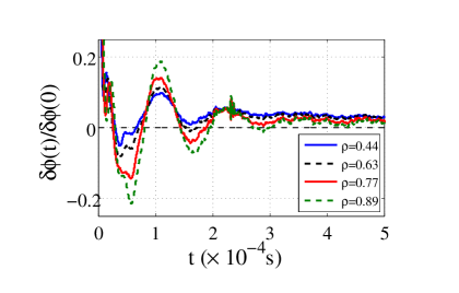
Figure 8: Normalized zonal potential ($\delta\phi$ component) versus time at four radial positions ($\rho\!=\!$0.44, 0.63, 0.77, 0.89)

The GAM-like oscillation is quickly damped, while the LFO lives for longer times. A fit of the time traces to a model,

$$\frac{\delta\phi(t)}{\delta\phi(0)}=A\,{\cos(2\pi ft+\Delta)}e^{-\gamma t}+R+f/(1+kt^{g})\,,$$ (10)

allows us to extract the frequency ($f$), amplitude of oscillations ($A$) and also the damping rate ($\gamma$) and residual level ($R$). A simple Fourier spectrum of the time traces gives also information of the frequency of oscillation and its amplitude but provides no information about the damping rate. The initial part ($t\!<\!25\,\mu$s) is skipped in the fit to avoid the short-lived GAM oscillation.

The obtained amplitudes are shown in figure 9 for several radial positions and several times during the ramp-up, together with the evolution of the neoclassical $E_{r}$. The error bars correspond to the 95% of confidence level in the fitting.

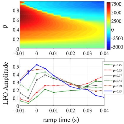
Figure 9: (top) Evolution of $E_{r}$ (color scale in V/m) during the numerical density ramp; (bottom) amplitude of the LFO obtained by fitting to Eq. 10 for several times in the ramp up and several radial positions.

For the outermost positions ($\rho\!\geq\!0.75$) the amplitude of the oscillations increases as time and density increases, reaches a maximum, and then decreases. The maximum is reached for times around $t=0$, the time at which the neoclassical electric field is close to zero at those radial locations. Finite orbit widths effects of the ambient $E_{r}$ are expected to enhance the damping of the LFO in helical systems [34] in consistency with previous simulations [35] for the TJ-II geometry. The maximum amplitude time delay observed for the different radial locations in figure 9 is due to the inward propagation of the region of small radial electric field associated to electron-to-ion root jump described in previous sections. Note that for the simulated density ramp the radial electric field does not change sign in the innermost positions which consequently do not show a maximum in the amplitude of the LFO.

It should be noted that the LFO amplitude increase close to the root jump observed in figure 9 and the neoclassical viscosity reduction discussed in previous sections are distinct. The latter was interpreted as a reduction of the linear dependence of neoclassical radial currents on the radial electric field, whereas the gyrokinetic simulations show the effects of a radially varying electric potential on the finite-width ion orbits.

To conclude this section it is worth mentioning that the characteristic frequencies of the LFO ($\sim 10$ kHz) are in the frequency range of the electric potential fluctuations observed experimentally to be correlated at long distances [7] and interpreted as zonal-flow structures [10]. The experimental characterization of these structures cast a radial scale of the order of $k\,r_{L}\!=\!0.1$, where $r_{L}$ is the ion Larmor radius, while the radial scale of the initial perturbation used in the simulation is larger, $k\,r_{L}\!=\!0.03$ (at $\rho\!=\!0.85$, close to the radial location of the probe measurements). Work is ongoing to study the relaxation of perturbations with a smaller radial scale (larger $k$), in order to compare them to the zonal flow evolution measured in reference [10].

7 Conclusions

The main result of this work is contained in Figures 1, 4 and 9. By solving the drift kinetic equation, we have been able to reproduce from first principles the evolution of the radial electric field during the low density transition associated with the formation of the shear layer in TJ-II. We have shown how in the electron root regime of stellarators, close to the transition to ion root, zonal flows are neoclassically undamped. During the change of root, the mean radial electric field goes through zero, a situation in which our gyrokinetic simulations predict larger zonal flow oscillations, in agreement with the experiment.

8 Acknowledgments

The authors thank the TJ-II team for their support. They are also grateful to R. Kleiber and R. Hatzky for developing the EUTERPE code and for their continuous assistance. This research was funded in part by grant ENE2012-30832, Ministerio de Economía y Competitividad, Spain.

9 Bibliography

References

- [1] K H Burrell. Effects of E x B velocity shear and magnetic shear on turbulence and transport in magnetic confinement devices. Physics of Plasmas, 4(5):1499–1518, 1997.
- [2] P W Terry. Suppression of turbulence and transport by sheared flow. Reviews of Modern Physics, 72:109–165, 2000.
- [3] F Wagner. A quarter-century of H-mode studies. Plasma Physics and Controlled Fusion, 49(12B):B1, 2007.
- [4] P Helander and A N Simakov. Intrinsic Ambipolarity and Rotation in Stellarators. Physical Review Letters., 101:145003, 2008.
- [5] I Calvo, F I Parra, J L Velasco, and J A Alonso. Stellarators close to quasisymmetry. Plasma Physics and Controlled Fusion, submitted, 2013. Available at arXiv:1307.3393 [physics.plasm-ph].
- [6] A Fujisawa, K Itoh, H Iguchi, K Matsuoka, S Okamura, A Shimizu, T Minami, Y Yoshimura, K Nagaoka, C Takahashi, M Kojima, H Nakano, S Ohsima, S Nishimura, M Isobe, C Suzuki, T Akiyama, K Ida, K Toi, S-I Itoh, and P H Diamond. Identification of zonal flows in a toroidal plasma. Physical Review Letters, 93:165002, 2004.
- [7] M A Pedrosa, C Silva, C Hidalgo, B A Carreras, R O Orozco, and D Carralero. Evidence of Long-Distance Correlation of Fluctuations during Edge Transitions to Improved-Confinement Regimes in the TJ-II Stellarator. Physical Review Letters, 100:215003, 2008.
- [8] K C Shaing. Stability of the radial electric field in a nonaxisymmetric torus. Physics of Fluids, 27(7):1567–1569, 1984.
- [9] B Ph van Milligen, M A Pedrosa, C Hidalgo, B A Carreras, T Estrada, J A Alonso, J L de Pablos, A Melnikov, L Krupnik, L G Eliseev, and S V Perfilov. The dynamics of the formation of the edge particle transport barrier at TJ-II. Nuclear Fusion, 51(11):113002, 2011.
- [10] J A Alonso, C Hidalgo, M A Pedrosa, B Van Milligen, D Carralero, and C Silva. Dynamic transport regulation by zonal flow-like structures in the TJ-II stellarator. Nuclear Fusion, 52(6):063010, 2012.
- [11] J L Velasco, J A Alonso, I Calvo, and J Arévalo. Vanishing neoclassical viscosity and physics of the shear layer in stellarators. Physical Review Letters, 109:135003, 2012.
- [12] G Jost, T M Tran, W A Cooper, L Villard, and K Appert. Global linear gyrokinetic simulations in quasi-symmetric configurations. Physics of Plasmas, 8(7):3321, 2001.
- [13] R Kleiber, R. Hatzky, A. Könies, K Kauffmann, and P. Helander. An improved control-variate scheme for particle-in-cell simulations with collisions. Computer Physics Communications, 182(4):1005, 2011.
- [14] F L Tabarés, B Bra nas, I García-Cortés, D Tafalla, T Estrada, and V Tribaldos. Edge characteristics and global confinement of electron cyclotron resonance heated plasmas in the TJ-II Stellarator. Plasma Physics and Controlled Fusion, 43(8):1023, 2001.
- [15] T Happel, T Estrada, and C Hidalgo. First experimental observation of a two-step process in the development of the edge velocity shear layer in a fusion plasma. Europhysics Letters, 84(6):65001, 2008.
- [16] C Hidalgo, M A Pedrosa, L García, and A Ware. Experimental evidence of coupling between sheared-flow development and an increase in the level of turbulence in the TJ-II stellarator. Physical Review E, 70:067402, 2004.
- [17] M A Pedrosa, B A Carreras, C Hidalgo, C Silva, M Hron, L García, J A Alonso, I Calvo, J L de Pablos, and J Stöckel. Sheared flows and turbulence in fusion plasmas. Plasma Physics and Controlled Fusion, 49(12B):B303, 2007.
- [18] J L Velasco and F Castejón. Study of the neoclassical radial electric field of the TJ-II flexible heliac . Plasma Physics and Controlled Fusion, 54(1):015005, 2012.
- [19] J L Velasco, K Allmaier, A López Fraguas, C D Beidler, H Maaßberg, W Kernbichler, F Castejón, and J A Jiménez. Calculation of the bootstrap current profile for the TJ-II stellarator. Plasma Physics and Controlled Fusion, 53(11):115014, 2011.
- [20] S.P. Hirshman and D.J. Sigmar. Neoclassical transport of impurities in tokamak plasmas. Nuclear Fusion, 21(9):1079, 1981.
- [21] S P Hirshman, K C Shaing, W I van Rij, C O Beasley, and E C Crume. Plasma transport coefficients for nonsymmetric toroidal confinement systems. Physics of Fluids, 29(9):2951–2959, 1986.
- [22] H Maaßberg, C D Beidler, and Y Turkin. Momentum correction techniques for neoclassical transport in stellarators. Physics of Plasmas, 16(7):072504, 2009.
- [23] J Arévalo, J A Alonso, K J McCarthy, and J L Velasco. Incompressibility of Impurity Flows in Low Density TJ-II Plasmas and Comparison with Neoclassical Theory. Nuclear Fusion, 53(2):023003, 2013.
- [24] B Zurro, A Baciero, D Rapisarda, and V Tribaldos. Comparison of Impurity Poloidal Rotation in ECRH and NBI Discharges of the TJ-II heliac. Fusion Science and Technology, 50(3):419–427, 2006.
- [25] S Satake, M Okamoto an N Nakajima, H Sugama, and M Yokoyama. Non-Local Simulation of the Formation of Neoclassical Ambipolar Electric Field in Non-Axisymmetric Configurations. Plasma and Fusion Research, 1:002, 2006.
- [26] K Hallatschek. Nonlinear three-dimensional flows in magnetized plasmas. Plasma Phys. Control. Fusion, 49:B137, 2007.
- [27] D Carralero, I Calvo, S da Grac̃a, B A Carreras, T Estrada, M A Pedrosa, and C Hidalgo. Shear-flow susceptibility near the low-density transition in TJ-II. Plasma Physics and Controlled Fusion, 54(6):065006, 2012.
- [28] K Itoh, S Toda, A Fujisawa, S-I Itoh, M Yagi, A Fukuyama, P H Diamond, and K Ida. Physics of internal transport barrier of toroidal helical plasmas. Physics of Plasmas, 14(2):020702, 2007.
- [29] L Guimarais, T Estrada, E Ascasíbar, M E Manso, L Cupido, T Happel, E Blanco, F Castejón, R Jiménez-Gómez, M A Pedrosa, C Hidalgo, I Pastor, and A López-Fraguas. Parametric dependence of the perpendicular velocity shear layer formation in TJ-II plasmas. Plasma and Fusion Research, 3:S1057–S1057, 2008.
- [30] Y Turkin, C D Beidler, H Maaßberg, S Murakami, V Tribaldos, and A Wakasa. Neoclassical transport simulations for stellarators. Physics of Plasmas, 18(2):022505, 2011.
- [31] M. N. Rosenbluth and F. L. Hinton. Poloidal Flow Driven by Ion-Temperature-Gradient Turbulence in Tokamaks. Physical Review Letters, 80:724, 1998.
- [32] A Mishchenko, P Helander, and A Könies. Collisionless dynamics of zonal flows in stellarator geometry. Physics of Plasmas, 15(7):072309, 2008.
- [33] S Satake, H Sugama, and T H Watanabe. Simulation studies on the GAM oscillation and damping in helical configurations. Nuclear Fusion, 47:1258, 2007.
- [34] A Mishchenko and R Kleiber. Zonal flows in stellarators in an ambient radial electric field. Physics of Plasmas, 19(7):072316, 2012.
- [35] E Sánchez. Simulation of zonal flow relaxation in the TJ-II heliac. Gyrokinetic Theory Working Group Meeting, Madrid, June 18-29, 2012.
- [36] E Sánchez, R Kleiber, R Hatzky, M Borchardt, P Monreal, F Castejón, A López-Fraguas, X Sáez, J L Velasco, I Calvo, A Alonso and D López-Bruna. Collisionless damping of flows in the TJ-II stellarator, Plasma Physics and Controlled Fusion, 55(1):014015, 2013.