On the density of shear transformation zones in amorphous solids

Abstract

We study the stability of amorphous solids, focussing on the distribution $P(x)$ of the local stress increase $x$ that would lead to an instability. We argue that this distribution is singular $P(x)\sim x^{\theta}$, where the exponent $\theta$ is non-zero if the elastic interaction between rearranging regions is non-monotonic, and increases with the interaction range. For a class of finite dimensional models we show that stability implies a lower bound on $\theta$, which is found to lie near saturation. For quadrupolar interactions these models yield $\theta\approx{0.6}$ for $d=2$ and $\theta\approx 0.4$ in $d=3$ where $d$ is the spatial dimension, accurately capturing previously unresolved observations in atomistic models, both in quasi-static flow and after a fast quench.

Dislocations play a key role in controlling plastic flow in crystalline solids. In contrast, the notion of defects is ill-defined in amorphous materials. However plasticity under shear in these materials occurs via events that are also well localized in space Argon (1979); Maloney and Lemaitre (2006); Picard et al. (2004). There are thus preferential locations where plastic rearrangements are likely to occur, which have been coined shear transformation zones (STZ)  Argon (1979), and are central to various proposed descriptions of plasticity Falk and Langer (1998). The microscopic nature of these objects is however elusive, and their concentration is thus hard to measure directly Rodney and Schuh (2009); Manning and Liu (2011). Recently it has been shown Wyart (2012); Lerner et al. (2013) in the particular case of packings of hard particles that the density $P(x)$ of excitations that rearrange if a local additional stress $x$ is applied is singular: $P(x)\sim x^{\theta}$, where the exponent $\theta$ is tuned such that small perturbations can have dramatic effects. This result raises the question of how stable generic amorphous solids are, and how this stability is reflected in the distribution of excitations $P(x)$. There is indirect evidence that $P(x)$ is indeed singular even when smooth interaction potentials are considered Karmakar et al. (2010): both following a quench and during steady flow, the increment where stress can be increased without plastic events in a system of $N$ particles scales as $N^{-\xi}$ where $\xi<1$. Assuming that the rearranging regions are independent would imply that $\theta>0$, as we shall recall below. However, the hypothesis of independence is inconsistent with observations at the yield stress Karmakar et al. (2010), raising doubts on the inference of $\theta$. Most importantly, what controls this singularity in the density of excitations is not known.

In this Letter we argue that the exponent $\theta$ is governed by the interaction between rearranging regions. $\theta$ can be non-zero if the interaction is non-monotonic, i.e. is either stabilizing or destabilizing depending on the location, and increases with increasing interaction range. We extend a previous mean-field, on-lattice model of plasticity Hébraud and Lequeux (1998) to the case of power-law interactions, and show that stability implies a lower bound on $\theta$, which is found to lie near saturation. When more realistic quadrupolar interactions are considered, which are known to characterize the far field effect of a plastic event Maloney and Lemaitre (2006); Picard et al. (2004), the model yields $\theta\approx{0.6}$ for $d=2$ and $\theta\approx 0.4$ in $d=3$, and reproduces at a surprising level of accuracy the system size dependence of the strain interval between plastic events observed in atomistic models Karmakar et al. (2010), both in flow and after a fast quench. Our findings suggest an explanation for puzzling differences between the depinning transition where an elastic manifold is driven in a random environment, and the yielding transition. They also support that popular models of plastic flow capture some aspects of the dynamics going on at the glass transition.

We consider cellular automaton models which are known to capture the critical behavior of the depinning transition Aragón et al. (2012) and have been used to study plastic flow Hébraud and Lequeux (1998); Baret et al. (2002); Zaiser (2006); Bocquet et al. (2009); Martens et al. (2012). The sample is decomposed into sites labeled by $i$, each carrying a scalar shear stress $\sigma_{i}$. A site represents a few particles. The applied shear stress is $\sigma=\frac{1}{N}\sum_{i}\sigma_{i}$. For each site we define a local threshold $\sigma_{i}^{th}$, which for simplicity is taken to be unity. If $\sigma_{i}>\sigma_{i}^{th}$, the site is mechanically unstable. When unstable, a site has a probability per unit time $1/\tau_{c}$ to rearrange plastically, in which case the local stress is set to zero. Physically, $\tau_{c}$ is the characteristic time to relax toward a new local minimum of energy. Such a plastic event affects the stress in the rest of the system, with a delay associated to elastic propagation. We shall neglect that this delay depends on the distance from the plastic event, and choose it to be exponentially distributed with mean $\tau_{r}$. A plastic event leads to the following change in the local stresses:

$$\sigma_{i} \rightarrow 0$$ (1)

$$\sigma_{j} \rightarrow \sigma_{j}+{\cal G}({\vec{r}}_{i}-{\vec{r}}_{j}).$$ (2)

In simple depinning models, ${\cal G}$ is strictly positive and the interaction is said to be monotonic. We focus here on non-monotonic interactions for which the sign of ${\cal G}$ varies. In this case if $\tau_{c}>0$, unstable sites can be re-stabilized by other plastic events. Such models predict the existence of a yield stress, and as we shall see are consistent with the Herschel-Bulkley relation:

$$\dot{\gamma}\sim(\sigma-\sigma_{c})^{\beta}$$ (3)

where the strain rate $\dot{\gamma}$ is defined as the number of collapses per unit time. In numerical simulations finite-size fluctuations can stop the dynamics even if $\sigma>\sigma_{c}$. When this happens we give small random kicks to every site until a new site becomes unstable. This method enables us to reach the steady state when $\sigma>\sigma_{c}$ and to study avalanche dynamics at $\sigma_{c}$.

We shall denote the distance to the yield stress of the site $i$ by $x_{i}\equiv 1-\sigma_{i}$. Our goal is to understand how the distribution $P(x)$ depends on the interaction ${\cal G}$. We introduce the decomposition $P(x)=P_{1}(x)+P_{2}(x)$ where $P_{2}(x)$ corresponds to collapsed sites, and $P_{1}(x)$ to the other sites.

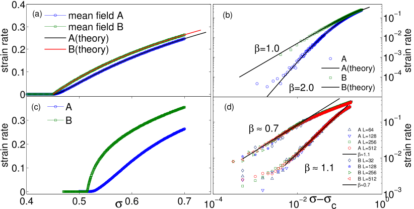
Figure 1: (color online). ${\dot{\gamma}}$ v.s. $\sigma$ for Models A and B (see text for details). Top panels: mean field interactions with $D=1/6$ on (a) linear and (b) log-log scales. Bottom panels: quadrupole interactions for $d=2$ on (c) linear and (d) log-log scales. The fits give $\beta\approx 1.1$, $\sigma_{c}\approx 0.52$ for model A and $\beta\approx 0.7$, $\sigma_{c}\approx 0.515$ for model B.

We first consider a solvable mean-field model where it is assumed that a plastic event leads to random kicks of stress that do not depend on position:

$${\cal G}_{mean}({\vec{r}}_{i}-{\vec{r}}_{j})=\frac{\eta_{j}}{\sqrt{N}}+\frac{\tilde{\eta}}{N}$$ (4)

where the $\eta_{j}$ are independent variables in space, and are not correlated from one plastic event to the next. They are randomly distributed in $[-\eta_{0},\eta_{0}]$, and $\eta_{0}$ does not depend on $N$ to ensure the existence of a thermodynamic limit. $\tilde{\eta}$ is chosen at each collapse event to ensure that the total stress is conserved, and thus depends on the random variables $\eta_{j}$ of that event. This model is a slight variation of that of Hebraud and Lequeux Hébraud and Lequeux (1998), and we shall briefly recall how to solve it.

In the thermodynamic limit Eq.(4) implies a Fokker-Planck equation for active sites:

$$\frac{\partial P_{1}(x)}{\partial t}=\\ \dot{\gamma}\Big{(}D\frac{\partial^{2}P_{1}(x)}{\partial x^{2}}+\lambda\frac{\partial P_{1}(x)}{\partial x}+\delta(x-1)\Big{)}-\theta(-x)\frac{P_{1}(x)}{\tau_{c}}$$ (5)

and an equation of similar form for $P_{2}(x)$ (see Appendix). $D\equiv\frac{\eta_{0}^{2}}{6}$ represents the diffusion constant of the local stress, coming from the random kicks of other collapsing sites. $\lambda$ is a Lagrange parameter that constrains the average stress, and is chosen such that $\int xP(x)dx=1-\sigma$. It results from the second term on the RHS of Eq.(4). The $\delta$ function term corresponds to the flux of reinserted sites at $\sigma=0$, equivalent to $x=1$. The last term in Eq.(5) corresponds to the flux of unstable sites that collapse, and $\theta(x)$ is the Heaviside function. Eq.(5), together with a similar equation for $P_{2}(x)$, are closed. We find (see Appendix) that no stationary solution with $\dot{\gamma}>0$ exists for $\sigma<\sigma_{c}=1/2-D$. The critical distribution ($\sigma=\sigma_{c}\implies\dot{\gamma}=0$) is independent of $\tau_{c}$ and $\tau_{r}$, and satisfies $P(x)\sim x$ for small $x$. This linear density of nearly unstable regions has a simple explanation: the stress in each site follows a diffusion equation. In the limit of small strain rate the instability threshold at $x=0$ becomes an absorbing boundary condition. In contrast, for monotonic problems such as pinned elastic interfaces, the distance to a local instability $x$ is always decreasing in time and $P(x)$ thus cannot vanish at $x=0$.

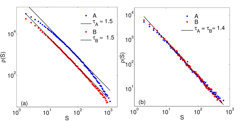
Figure 2: Distribution of avalanches size for (a) mean-field interaction and (b) quadrupole interactions.

Solving this mean field model at finite strain rate, we find at first order in $\dot{\gamma}$:

$$\begin{split}&\sigma-\sigma_{c}=\\ &(\frac{1}{2}+D)\sqrt{D\tau_{c}}\dot{\gamma}^{1/2}+[\tau_{r}(\frac{1}{2}+2D)+\frac{\tau_{c}}{4}+(1-D)D\tau_{c}]\dot{\gamma}\end{split}$$ (6)

We thus see that if $\tau_{c}\neq 0$, $\sigma-\sigma_{c}\sim\dot{\gamma}^{1/2}$, corresponding to $\beta=2$ in Eq.(3), also obtained in the model of Hébraud and Lequeux (1998). However if $\tau_{c}=0$, $\sigma-\sigma_{c}\sim\dot{\gamma}$, corresponding to $\beta=1$. These results are tested numerically for Model A ($\tau_{r}=0,\tau_{c}=1$) and Model B ($\tau_{r}=1,\tau_{c}=0$) in Fig.(1). Despite the notable difference between $A$ and $B$, $P_{c}(x)$ is independent of the choice of dynamics. This supports that the class of models we consider should yield correct values for $\theta$, but indicates that our assumption that the delay $\tau_{r}$ is independent of position may yield incorrect Herschel-Bulkley exponents. Interestingly, we find at $\sigma_{c}$ that the avalanches distribution $\rho(S)$, where $S$ is the number of plastic events, follows $\rho(S)\sim 1/S^{\tau}$ with $\tau\approx 3/2$ independently of the choice of dynamics, as shown in Fig.(2). This result is consistent with mean-field depinning Fisher (1998) and the ABBM model Alessandro et al. (1990).

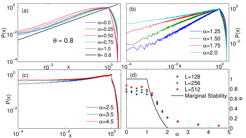
Figure 3: (color online). $P(x)$ v.s. $x$ for a $d=2$ system with power-law interaction of Eq.(7): (a) When $\alpha\leq 1$, $\theta\geq 0.8$ (b) When $1<\alpha\leq 2$, $\theta$ decreases as $\alpha$ increases. (c) When $\alpha>2$, $\theta\approx 0$. (d) $\theta$ vs $\alpha$ obtained in our simulation and compared with the theoretical lower bound of Eq.(On the density of shear transformation zones in amorphous solids).

To study finite dimensional effects, we now consider interactions decaying with distance, of the form:

$${\cal G}_{mean}({\vec{r}}_{i}-{\vec{r}}_{j})=\frac{\eta_{j}}{r_{ij}^{\alpha}}+\eta_{1}$$ (7)

where $\eta_{j}\in[-\eta,\eta]$ is a random variable uniformly distributed, and $\eta_{1}$ is again a global shift to keep the average stress constant. To ensure that the diffusion constant stemming from plastic events has a thermodynamic limit, the coefficient $\eta$ must be such that $\int_{1}^{L}\frac{\eta^{2}}{r^{2\alpha}}d^{d}r\sim 1$ where $d$ is the spatial dimension and $L$ the linear system size. We get $\eta\sim L^{\alpha-d/2}$ for $\alpha<d/2$, $\eta\sim 1/\sqrt{\ln L}$ for $\alpha=d/2$ and $\eta\sim 1$ for $\alpha>d/2$.

Computing $\theta$ is now a much harder problem. However we now show that stability implies a bound on this exponent. Let us denote by $m$ the average number of plastic events that are triggered if one single event at the origin takes place. We assume that the distribution $P(x)$ satisfies $P(x)\sim x^{\theta}$. A site at a distance $r$ experiences a kick which contains the term $\eta_{1}$ of order $1/N$ that stems from stress conservation and a term $\eta/r^{\alpha}$, which is destabilizing or stabilizing with probability $1/2$. The term $\eta_{1}\sim 1/N$ will destabilize the site with a probability $p_{1}\sim P(x<1/N)\sim N^{-(1+\theta)}$, so that overall in the entire system this will trigger of the order of $N^{-\theta}$ events, which is negligible as long as $\theta>0$. The probability $p_{2}(r)$ that the term $\eta/r^{\alpha}$ destabilizes the site is of order $p_{2}(r)=P(x\leq\eta/r^{\alpha})/2\sim\eta^{\theta+1}/r^{\alpha(\theta+1)}$. Integrating over all sites we get:

$$m\sim\eta^{\theta+1}\int_{1}^{L}\frac{dr}{r^{\alpha(\theta+1)+1-d}}\sim\eta^{\theta+1}L^{d-\alpha(\theta+1)}\sim L^{\nu}$$ (8)

where the exponent $\nu$ can be computed from the dependence of $\eta$ with $L$. Stability toward run-away avalanches requires $\nu\leq 0$, which finally leads to:

$$\theta \geq 1\ \ \ \ \ \ \ \ \ \hbox{ if}\ d\geq 2\alpha$$

$$\theta \geq \frac{d}{\alpha}-1\ \ \ \hbox{ if}\ d/2\leq\alpha\leq d$$ (9)

$$\theta \geq 0\ \ \ \ \ \ \ \ \ \ \hbox{ if }\ \alpha>d$$

This prediction is tested in Fig.(3), where $P(x)$ is shown for various interaction range $\alpha$ in two dimensions, from which the exponent $\theta$ is extracted. Fig.(3.d) shows the comparison between the measurement and the stability bound. For $\alpha<1$ the bound appears slightly violated, but less and less so for larger system sizes, supporting that $\theta=1$, as we predicted exactly for $\alpha=0$. For larger $\alpha$, $\theta$ is found to lie close to the bound but systematically above, although our data cannot rule out saturation. Our analysis thus implies that the range of interaction is a key determinant of $P(x)$ and $\theta$, and that for this class of models, systems lie close to marginal stability.

Finally we consider the more realistic case where the interaction is not random, but quadrupolar in the far field Picard et al. (2004). Our model then belongs to the class of elastoplastic models Bocquet et al. (2009); Talamali et al. (2011); Zaiser (2006); Martens et al. (2012). In two dimensions for a simple shear along the $x$ axis one has for an infinite system ${\cal G}(r)=\frac{\cos{4\phi}}{r^{2}}$, where $\phi$ is the angle made with the $x$ axis. Periodic boundary conditions can be implemented using the Fourier representation, ${\cal G}(k_{x},k_{y})=k_{x}^{2}k_{y}^{2}/k^{4}$, and the discrete wave vectors, $k_{x}=2\pi n_{x}/L$,$k_{y}=2\pi n_{y}/L$. This interaction can be computed also in $d=3$ where it decays as ${\cal G}(r)\sim 1/r^{3}$.

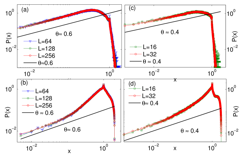
Figure 4: (color online). $P(x)$ v.s. $x$ (a) for $d=2$ at the critical stress, (b) for $d=2$ after a fast quench (c) for $d=3$ at the critical stress and (d) for $d=3$ after a fast quench. Results are shown for dynamics A, and are identical for dynamics B.

To our knowledge the exponent $\beta$ of Eq.(3) has not been computed for such models. Our results are shown in Fig.(1) bottom for dynamics A and B, and are well-captured by the Herschel-Bulkley law with $\beta_{A}\approx 1.1$ and $\beta_{B}\approx 0.7$. We also compute the avalanche exponent and find $\tau\approx 1.42$ in both dynamics, again close to the mean field value $1.5$ in agreement with Zaiser (2006) but somewhat larger than Talamali et al. (2011), as shown in Fig.(2).

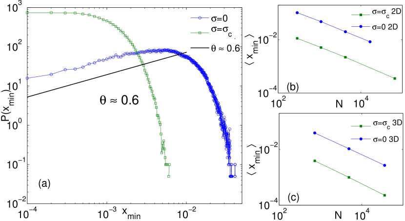
Figure 5: (color online). Left: distribution of the most unstable site $P(x_{\rm min})$ at $\sigma_{c}$ (green square) and after a rapid quench, at $\sigma=0$, (blue circles) for $d=2$. Right: Evolution of $\langle x_{\rm min}\rangle$ v.s. $N$ indicating a power law regime $\langle x_{\rm min}\rangle\sim N^{-\xi}$ with $\xi\approx 0.63$ in $d=2$ and $\xi\approx 0.71$ in $d=3$ both for $\sigma_{c}$ and the rapid quench.

One central result concerns the density of excitations $P(x)$. We measure this quantity in two situations: (i) at the yield stress $\sigma_{c}$, in the steady state (ii) at $\sigma=0$ after a ”quench” which mimics the behavior that would occur if the temperature was suddenly set to zero in a liquid. In the latter case the initial local stress, $\sigma_{i}$, are drawn from a Gaussian symmetric distribution $Q_{0}(\sigma)$, so that $\sigma=0$. The system is however unstable because many sites with $|\sigma_{i}|>1$ can collapse and trigger other rearrangements. This dynamics stops when $|\sigma_{i}|<1$ on all sites. Our results are shown in Fig.(4). We find that $\theta\approx 0.6$ in two dimensions and $\theta\!\approx\!0.4$ in three dimensions, both at $\sigma_{c}$ and after the quench at $\sigma=0$.

Can such a simple model, that neglects in particular the tensorial nature of stress, capture essential aspects of the glassy dynamics that occurs during an isotropic quench? To test this hypothesis we compare our results with the atomistic simulations of Karmakar et al. (2010). $P(x)$ is not available directly, but the statistics of $x_{\rm min}$ can be obtained accurately by considering the minimal increment of strain, or stress, required to generate a plastic event. It is found that $\langle x_{\rm min}\rangle\sim N^{-\xi}$ with $\xi\!\approx\!0.62$ after a quench, and $\xi\!\approx\!2/3$ at the yield stress, with no clear dependence on the dimension. Our measurement of the exponent $\xi$ are shown in Fig.(5), and are remarkably similar to these observations, as we find $\xi\!\approx\!0.63$ in $d=2$ and $\xi\approx 0.71$ in $d=3$ both after a quench at $\sigma=0$ or in the steady state at $\sigma_{c}$. The exponent $\xi$ can be related to $\theta$ if one assumes the independence of the variables $x_{i}$.

$$\int_{0}^{\langle x_{\rm min}\rangle}\,dx\,P(x)\sim\frac{1}{N}\;\to\;\langle x_{\rm min}\rangle\sim N^{-\frac{1}{\theta+1}}$$ (10)

leading to $\theta=1/\xi-1$, a relationship satisfied in our data. The independence assumption also implies a specific form for the distribution of the most unstable site at small argument $P(x_{\rm min})\!\sim\!x_{\rm min}^{\theta}$, which is indeed observed in Karmakar et al. (2010) for quenched systems, but not in quasistatic flow, where $P(x_{\rm min})\!\sim\!x_{\rm min}^{0}$ was found. Our measurement of $P(x_{\rm min})$ shown in Fig.(5) are strikingly similar to Karmakar et al. (2010), and displays precisely these features, supporting the validity of our approach. Our finding that the relationship $\theta=1/\xi-1$ holds despite that the lack of strict independence indicates that $\theta$ can be reliably extracted from size effects, and may thus be accessible experimentally.

Conclusion: The phenomenology of the depinning transition (see Fisher (1998); Le Doussal et al. (2002) for a review) of an elastic interface is very similar to that of the much less understood yield stress transition Zaiser (2006); Talamali et al. (2011): there is a critical force $F_{c}$ where the dynamics also consists of power-law avalanches. At larger forces, the velocity follows $V\sim(F-F_{c})^{\beta}$, a form equivalent to the Herschel-Bulkley relation. There are several important differences however. First, for depinning $\beta\leq 1$ ($\beta=1$ is the mean field result), whereas yield stress materials generally display $\beta>1$. Here we have shown that models where unstable sites can be re-stabilized, which occurs for non-monotonic interactions and $\tau_{c}>0$, can indeed present $\beta>1$. Second, in depinning the number of avalanches triggered when $F$ is slightly increased below $F_{c}$ is extensive and not singular near the transition. This fact allows one to obtain the exponent $\tau$ characterizing avalanches Narayan and Fisher (1993); Aragón et al. (2012). Near the yield stress transition, atomistic simulations Salerno et al. (2012) support that this hypothesis does not hold, and that the number of avalanches triggered at $\sigma_{c}$ depends on the volume with a non-trivial exponent. We interpret that difference as stemming from the fact that $\theta=0$ for depinning, whereas the long range and non-monotonicity of the interactions allow $\theta>0$ for the yielding transition, implying a non-trivial relationship between stress increase and number of avalanches triggered. This result supports that the exponent $\theta$ should enter in a yet-to be done scaling description of the yielding transition. This exponent also described materials after a isotropic quench, and may thus also play a role near the glass transition. This point of view emphasizes the role of elastic interactions, often neglected in theories of the glass transition, but which have recently been proposed to control the fragility of liquids Yan et al. (2013).

Acknowledgments: it is a pleasure to thank G. Düring, Le Yan, and Eric DeGiuli for comments on the manuscript. This work has been supported by the Sloan Fellowship, NSF CBET-1236378, NSF DMR-1105387, and Petroleum Research Fund #52031-DNI9. This work was also supported partially by the MRSEC Program of the National Science Foundation under Award Number DMR-0820341, and the hospitality of the Aspen Center for Physics.

Appendix A Appendix: solution of the mean-field model

We give here a few more details about the solution of the mean-field case. We write the distribution $P(x)$ as $P(x)=P_{1}(x)+P_{2}(x)$, where $P_{1}(x)$ is the distribution of stable ($x>0$) and mechanically unstable ($x<0$) sites, and $P_{2}(x)$ is the distribution of collapsed sites. In the thermodynamic limit, $P_{1}$ and $P_{2}$ satisfy the Fokker-Planck equations

$$\frac{\partial P_{1}(x)}{\partial t}=\\ \dot{\gamma}\Big{(}D\frac{\partial^{2}P_{1}(x)}{\partial x^{2}}+\lambda\frac{\partial P_{1}(x)}{\partial x}+\delta(x-1)\Big{)}-\theta(-x)\frac{P_{1}(x)}{\tau_{c}}$$ (11)

$$\frac{\partial P_{2}(x)}{\partial t}=\\ \dot{\gamma}\Big{(}D\frac{\partial^{2}P_{1}(x)}{\partial x^{2}}+\lambda\frac{\partial P_{1}(x)}{\partial x}\Big{)}+\theta(-x)\frac{P_{1}(x)}{\tau_{c}}-\frac{P_{2}(x)}{\tau_{r}}$$ (12)

In the stationary limit, these two equations imply, by taking the integral of (11) and ($\ref{AFP2})$, the following conservation law :

$$\dot{\gamma}=\frac{\int_{-\infty}^{\infty}P_{2}(x)dx}{\tau_{r}}=\frac{\int_{-\infty}^{0}P_{1}(x)dx}{\tau_{c}}$$ (13)

This equality simply states that in a stationary state, the flux of collapsing site is equal to the flux of sites that become stabilized again. Solving (11) gives $P_{1}$ up to a constant, which we can then determine thanks to (13), using the normalization of the complete distribution $P$. We find the critical value $\lambda_{c}=1$ above which there exists a stationary solution with $\dot{\gamma}>0$. The same equation 13 allows to solve for $\dot{\gamma}$ as a function of $\lambda-\lambda_{c}$. Expanding for $\lambda\simeq\lambda_{c}$ gives :

$$\dot{\gamma}=\frac{(\lambda-\lambda_{c})^{2}}{D\tau_{c}}-\frac{(\tau_{c}+2\tau_{r})(\lambda-\lambda_{c})^{3}}{D^{2}\tau_{c}^{2}}+O(\lambda-\lambda_{c})^{4}$$ (14)

We then have to relate $\lambda-\lambda_{c}$ and $\sigma-\sigma_{c}$, which is done using that $\int_{-\infty}^{+\infty}xP(x)dx=1-\sigma$. Multiplying (12) by $x$ and integration by parts yields :

$$\int_{-\infty}^{+\infty}xP_{2}(x)dx=\frac{\tau_{r}}{D\tau_{c}}(\lambda_{c}-\lambda)^{3}$$ (15)

and because we have already computed $P_{1}$, we can compute the expansion of $\sigma-\sigma_{c}$ in terms of $\lambda-\lambda_{c}$. A few straightforward computations finally yield (6).

References

- Argon (1979) A. Argon, Acta Metallurgica 27, 47 (1979).
- Maloney and Lemaitre (2006) C. E. Maloney and A. Lemaitre, Phys. Rev. e 74, 016118 (2006).
- Picard et al. (2004) G. Picard, A. Ajdari, F. Lequeux, and L. Bocquet, The European Physical Journal E 15, 371 (2004).
- Falk and Langer (1998) M. L. Falk and J. S. Langer, Phys. Rev. E 57, 7192 (1998).
- Rodney and Schuh (2009) D. Rodney and C. Schuh, Phys. Rev. Lett. 102, 235503 (2009).
- Manning and Liu (2011) M. L. Manning and A. J. Liu, Phys. Rev. Lett. 107, 108302 (2011).
- Wyart (2012) M. Wyart, Phys. Rev. Lett. 109, 125502 (2012).
- Lerner et al. (2013) E. Lerner, G. Düring, and M. Wyart, Soft Matter , (2013).
- Karmakar et al. (2010) S. Karmakar, E. Lerner, and I. Procaccia, Phys. Rev. E 82, 055103 (2010).
- Hébraud and Lequeux (1998) P. Hébraud and F. Lequeux, Phys. Rev. Lett. 81, 2934 (1998).
- Aragón et al. (2012) L. E. Aragón, E. A. Jagla, and A. Rosso, Phys. Rev. E 85, 046112 (2012).
- Baret et al. (2002) J.-C. Baret, D. Vandembroucq, and S. Roux, Phys. Rev. Lett. 89, 195506 (2002).
- Zaiser (2006) M. Zaiser, Advances in Physics 55, 185 (2006).
- Bocquet et al. (2009) L. Bocquet, A. Colin, and A. Ajdari, Physical review letters 103 (2009).
- Martens et al. (2012) K. Martens, L. Bocquet, and J.-L. Barrat, Soft Matter 8, 4197 (2012).
- Fisher (1998) D. S. Fisher, Physics Reports 301, 113 (1998).
- Alessandro et al. (1990) B. Alessandro, C. Beatrice, G. Bertotti, and A. Montorsi, Journal of Applied Physics 68, 2901 (1990).
- Talamali et al. (2011) M. Talamali, V. Petäjä, D. Vandembroucq, and S. Roux, Phys. Rev. E 84, 016115 (2011).
- Le Doussal et al. (2002) P. Le Doussal, K. J. Wiese, and P. Chauve, Phys. Rev. B 66, 174201 (2002).
- Narayan and Fisher (1993) O. Narayan and D. S. Fisher, Phys. Rev. B 48, 7030 (1993).
- Salerno et al. (2012) K. M. Salerno, C. E. Maloney, and M. O. Robbins, Phys. Rev. Lett. 109, 105703 (2012).
- Yan et al. (2013) L. Yan, G. Düring, and M. Wyart, PNAS 110, 6307 (2013).