Scalar, spinor, and photon fields under relativistic cavity motion

Abstract

We analyse quantised scalar, spinor, and photon fields in a mechanically rigid cavity that is accelerated in Minkowski spacetime, in a recently introduced perturbative small-acceleration formalism that allows the velocities to become relativistic, with a view to applications in relativistic quantum information. A scalar field is analysed with both Dirichlet and Neumann boundary conditions, and a photon field under perfect conductor boundary conditions is shown to decompose into Dirichlet-like and Neumann-like polarisation modes. The Dirac spinor is analysed with a nonvanishing mass and with dimensions transverse to the acceleration, and the MIT bag boundary condition is shown to exclude zero modes. Unitarity of time evolution holds for smooth accelerations but fails for discontinuous accelerations in spacetime dimensions $(3+1)$ and higher. As an application, the experimental desktop mode-mixing scenario proposed for a scalar field by Bruschi et al. [New J. Phys. 15, 073052 (2013)] is shown to apply also to the photon field.

I Introduction

A relativistic quantum field is affected by the kinematics of the spacetime in which the field lives. Well-known examples are the Hawking and Unruh effects, associated with black holes and accelerated observers hawking ; unruh ; Crispino:2007eb , the dynamical (or nonstationary) Casimir effect (DCE) moore-dyncas ; Reynaud1 ; Dodonov:advchemphys ; Dodonov:2010zza , associated with moving boundaries, and cosmological particle creation parker-I ; parker-II . Similar effects have been predicted to occur in condensed matter laboratory systems, where the prospects of experimental verification may be significantly better Barcelo:2005fc . The effects could be potentially harnessed to serve quantum information tasks, with current and near-foreseeable technology, including quantum communication between satellites Rideout:2012jb .

In this paper we consider a quantum field confined in a cavity that moves in Minkowski spacetime. The cavity is assumed to be mechanically rigid, as seen in its instantaneous rest frame, and the acceleration is assumed to be small in magnitude, compared with the inverse linear dimensions of the cavity. Under these assumptions the evolution of a scalar field in the cavity can be solved in a recently developed formalism that treats the acceleration perturbatively but allows the velocities, the travel times, and the travel distances to remain arbitrary, and in particular allows the velocities to become relativistic Bruschi:2011ug ; Bruschi:2012pd ; Bruschi:2013vk . For acceleration with constant direction, the notion of a relativistic rigid body can be implemented to all orders in the perturbative expansion, and for acceleration with varying direction, the formalism has been developed to first order in the acceleration without relativistic ambiguities Bruschi:2012pd .

While this small acceleration formalism overlaps in part with situations covered by the small distance approximations often considered in the DCE literature Dodonov:advchemphys ; Dodonov:2010zza , and by other approximation schemes DalvitMazzitelli1999 ; AlvesGranhenPires2010 , its novelty is in the ability to accommodate relativistic velocities in a systematic fashion. Applications to quantum information tasks in relativistic or potentially relativistic contexts have been analysed in Bruschi:2011ug ; Bruschi:2012pd ; Bruschi:2013vk ; Friis:2011yd ; Friis:2012tb ; Bruschi:2012uf ; Alsing:Fuentes:2012 ; Friis:2012ki ; Friis:2012nb ; Friis:2012cx . In particular, the formalism is applicable to a cavity whose motion is implemented by superconducting quantum interference device (SQUID) circuits without mechanically moving parts Friis:2012cx . A generalisation to massless fermions in a $(1+1)$-dimensional cavity is given in Friis:2011yd .

The main purpose of this paper is to adapt the analysis of a scalar field in the cavity to the electromagnetic field, with perfect conductor boundary conditions at the cavity walls. The interest of this question arises from the traditional prime suspect role of the electromagnetic field in experimental scenarios that involve acceleration effects moore-dyncas ; Reynaud1 ; Dodonov:advchemphys ; Dodonov:2010zza , including the recent experiments in which acceleration is simulated by SQUID circuits wilson-etal . We find that the electromagnetic field decomposes into two sets of polarisation modes, one similar to a Dirichlet scalar field and the other similar to a Neumann scalar field. The results for the evolution of the electromagnetic field hence follow in a straightforward fashion from those for the Dirichlet scalar field, found in Bruschi:2011ug ; Bruschi:2012pd , and those for the Neumann scalar field, which we provide in this paper. In particular, our results confirm that the experimental scenario of a cavity accelerated on a desktop, proposed and analysed for a scalar field in Bruschi:2012pd , applies also to the photon field.

A second purpose is to address a Dirac spinor at a generality that covers a $(3+1)$-dimensional cavity, generalising the case of a massless $(1+1)$ field analysed in Friis:2011yd . This question is motivated by the prospect of simulating acceleration effects for fermions in solid state analogue systems boada:dirac ; ZhangWangZhu2012 ; Iorio2012 . After finding the general family of boundary conditions that ensures a vanishing probability current through the walls, we specialise to the MIT bag boundary condition Chodos:1974je ; Elizalde:1997hx , which arises when the cavity field is matched to a highly massive field in the exterior and the exterior mass is taken to infinity. We find that the MIT bag boundary condition leads to a charge conjugation symmetric spectrum without zero modes, independently of the field mass or of effects from dimensions transverse to the acceleration. We also present the explicit Fourier transform formulas for the Bogoliubov coefficients in the case when the acceleration varies smoothly in time, generalising the scalar field formulas given in Bruschi:2012pd . We use the insights gathered about the fermionic Bogoliubov transformations to comment on the implications for quantum information purposes, such as discussed in Friis:2011yd ; Friis:2012tb ; Friis:2012ki .

A third purpose is to examine whether the time evolution of the cavity field is implementable as a unitary transformation in the Fock space. (We thank Pablo Barberis-Blostein and Ivette Fuentes for drawing our attention to this question.) As the potential failure of unitarity is governed by the deep ultraviolet regime of the theory, the issue here is whether any predictions computed from the formalism are sensitive to the idealisations made in the ultraviolet. Comfortingly, we find that the evolution is unitary whenever the acceleration varies smoothly in time. In the limit of discontinuous acceleration, unitarity however fails in spacetime dimensions $(3+1)$ and higher.

A fourth purpose is to give a proper justification to certain technical properties that have been stated and utilised in earlier papers Bruschi:2011ug ; Bruschi:2012pd ; Bruschi:2013vk ; Friis:2011yd ; Friis:2012tb ; Bruschi:2012uf ; Alsing:Fuentes:2012 ; Friis:2012ki ; Friis:2012nb ; Friis:2012cx . In particular, we explain how the direction of the acceleration comes to be encoded in the Bogoliubov coefficient formulas.

We begin in Section II by recalling the Dirichlet scalar field analysis that was outlined in Bruschi:2011ug , establishing the notation for the rest of the paper. The Neumann scalar field is addressed in Sec. III. The electromagnetic field is addressed in Secs. IV and V, and the Dirac field in Sec. VI. Unitarity of the evolution is analysed in Sec. VII, with auxiliary asymptotic estimates deferred to the Appendix. The results are summarised and discussed in Sec. VIII.

Our metric signature is mostly plus, and we use units in which $c=\hbar=1$.

II $(1+1)$ Dirichlet scalar field

In this section we address a real scalar field of strictly positive mass in $(1+1)$-dimensional Minkowski spacetime, with Dirichlet boundary conditions at the cavity walls. While the core results can be found in earlier short format papers Bruschi:2011ug ; Bruschi:2012pd ; Bruschi:2013vk ; Bruschi:2012uf , our purpose here is to be sufficiently self-contained to allow a direct comparison to the Maxwell field analysis in Sec. V.

II.1 Inertial cavity

Let $\phi$ be a real scalar field of mass ${\mu}>0$ in $(1+1)$-dimensional Minkowski spacetime, satisfying the Klein-Gordon equation

$$\left(-\square+{\mu}^{2}\right)\phi=0\ ,$$ (II.1)

where $\square$ is the scalar Laplacian. The field is confined in a cavity that may move but maintains a prescribed length $L>0$ in its instantaneous rest frame. The field is assumed to satisfy Dirichlet boundary conditions at the cavity walls.

When the cavity is inertial, we may introduce Minkowski coordinates $(t,z)$ in which the metric reads

$$ds^{2}=-dt^{2}+dz^{2}\ ,$$ (II.2)

and the walls are, respectively, at $z=z_{0}$ and $z=z_{1}:=z_{0}+L$, dragged along the timelike Killing vector $\partial_{t}$. $z_{0}$ could be set to zero without loss of generality, but leaving $z_{0}$ unspecified for the moment will be useful for matching to accelerated motion below.

The Klein-Gordon inner product takes the form

$$(\phi_{1},\phi_{2})=-i\int_{z_{0}}^{z_{1}}\phi_{1}\overleftrightarrow{\partial_{t}}\>\overline{\phi_{2}}\,dz\ ,$$ (II.3)

where the overline denotes complex conjugation (we adopt the conventions of byd in which the inner product is antilinear in the second argument). A standard basis of field modes that are of positive frequency with respect to $\partial_{t}$ and orthonormal in the Klein-Gordon inner product (II.3) is

$$\phi^{M}_{n}(t,z) :=\frac{1}{\sqrt{\omega_{n}L}}\sin\!\left(\frac{n\pi(z-z_{0})}{L}\right)e^{-i\omega_{n}t}\ ,$$ (II.4a)

$$\omega_{n} :=\sqrt{{\mu}^{2}+{(\pi n/L)}^{2}}\ ,$$ (II.4b)

where $n=1,2,\ldots$. The phase in (II.4a) has been chosen so that $\partial_{z}\phi^{M}_{n}|_{z=z_{0}}>0$ at $t=0$.

II.2 Uniformly accelerated cavity

When the cavity is uniformly accelerated, in the sense of being dragged along a boost Killing vector, we may introduce Rindler coordinates $(\eta,\chi)$ takagi in which

$$ds^{2}=-\chi^{2}\,d\eta^{2}+d\chi^{2}\ ,$$ (II.5)

with $-\infty<\eta<\infty$ and $0<\chi<\infty$, and the cavity walls are, respectively, at $\chi=\chi_{0}>0$ and $\chi=\chi_{1}:=\chi_{0}+L$. The boost Killing vector is $\partial_{\eta}$. It is convenient to parametrise the geometry of the accelerated cavity by the pair $(h,L)$, where the dimensionless parameter $h$ lies in the interval $0<h<2$, such that

$$\chi_{0} =\left(\frac{1}{h}-\frac{1}{2}\right)\!L\ ,$$ (II.6a)

$$\chi_{1} =\left(\frac{1}{h}+\frac{1}{2}\right)\!L\ .$$ (II.6b)

The proper acceleration at the centre of the cavity, at $\chi=(\chi_{0}+\chi_{1})/2$, equals $h/L$. Note that the proper acceleration is not uniform within the cavity: each worldline of constant $\chi$ has proper acceleration $1/\chi$, and the proper accelerations at the cavity walls are hence, respectively, $1/\chi_{0}$ and $1/\chi_{1}$. The upper bound on $h$ comes from the condition that the proper acceleration at both cavity walls remain finite.

The Klein-Gordon inner product takes the form

$$(\phi_{1},\phi_{2})=-i\int_{\chi_{0}}^{\chi_{1}}\phi_{1}\overleftrightarrow{\partial_{\eta}}\>\overline{\phi_{2}}\,\chi^{-1}\,d\chi\ .$$ (II.7)

By separation of variables takagi , we find that a basis of field field modes that are of positive frequency with respect to $\partial_{\eta}$ and orthonormal in the Klein-Gordon inner product (II.7) is

$$\begin{aligned} \mathllap{\phi^{R}_{n}(\eta,\chi)}&\phantom{:}=f_{n}(\chi)e^{-i\Omega_{n}\eta}\ ,\end{aligned}$$ (II.8a)

$$\begin{aligned} \mathllap{f_{n}(\chi)}&:=N_{n}\big{[}I_{-i\Omega_{n}}({\mu}\chi_{0})I_{i\Omega_{n}}({\mu}\chi)\\ &\hskip 42.67912pt-I_{i\Omega_{n}}({\mu}\chi_{0})I_{-i\Omega_{n}}({\mu}\chi)\big{]}\ ,\end{aligned}$$ (II.8b)

where $n=1,2,\ldots$, $I$ is the modified Bessel function of the first kind nist-dig-library , the eigenfrequencies $\Omega_{n}$ are determined by the boundary condition $\phi^{R}_{n}(\eta,\chi_{1})=0$ and are ordered so that $0<\Omega_{1}\leq\Omega_{2}\leq\cdots$, and $N_{n}$ is a normalisation constant. We shall return to the phase choice of $N_{n}$ in subsection II.3.

Note that both $\eta$ and $\Omega_{n}$ are dimensionless. As the proper time at the centre of the cavity equals $L\eta/h$, the angular frequency of $\phi^{R}_{n}$ with respect to this proper time is $h\Omega_{n}/L$.

II.3 Matching

Consider now a cavity whose motion turns instantaneously from inertial to uniform acceleration, so that the wall velocities are continuous but the proper accelerations have a finite discontinuity. We take the inertial segment to be as in subsection II.1 for $t\leq 0$ and the uniformly accelerated segment to be as in subsection II.2 for $\eta\geq 0$.

To begin with, suppose that the acceleration is towards increasing $z$. The transformation relating the Minkowski and Rindler coordinates is then takagi

$$t =\chi\sinh\eta\ ,$$ (II.9a)

$$z =\chi\cosh\eta\ ,$$ (II.9b)

and the cavity wall loci at $t=0$ in the two coordinate systems are related by $z_{0}=\chi_{0}$ and $z_{1}=\chi_{1}$, as shown in Fig. 1.

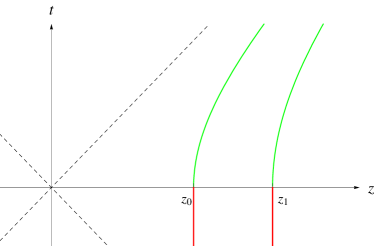
Figure 1: Matching an inertial cavity to a uniformly accelerating cavity in $(1+1)$-dimensional Minkowski space, in the global Minkowski coordinates $(t,z)$. For $t\leq 0$ the cavity is inertial, following the orbits of the time translation Killing vector $\partial_{t}$: the world lines of the walls are, respectively, $z=z_{0}$ and $z=z_{1}$, where $0<z_{0}<z_{1}$. For $t\geq 0$ the cavity is uniformly accelerated towards increasing $z$, in the sense that it follows the orbits of the boost Killing vector $z\partial_{t}+t\partial_{z}$: the world lines of the walls are, respectively, $z=\sqrt{z_{0}^{2}+t^{2}}$ and $z=\sqrt{z_{1}^{2}+t^{2}}$.

We write the Bogoliubov transformation from the Minkowski modes to the Rindler modes as

$$\phi^{R}_{m}=\sum_{n}\,\left({{}_{\text{o}}\alpha}_{mn}\phi^{M}_{n}+{{}_{\text{o}}\beta}_{mn}\overline{\phi^{M}_{n}}\right)\ .$$ (II.10)

From (II.10) and the orthonormality of the Minkowski modes, we have byd

$${{}_{\text{o}}\alpha}_{mn} =\bigl{(}\phi^{R}_{m},\phi^{M}_{n}\bigr{)}\ ,$$ (II.11a)

$${{}_{\text{o}}\beta}_{mn} =-\bigl{(}\phi^{R}_{m},\overline{\phi^{M}_{n}}\,\bigr{)}\ ,$$ (II.11b)

where the inner products may be evaluated by (II.3) at $t=0$ or equivalently by (II.7) at $\eta=0$. While these inner products do not appear to have expressions in terms of known functions, they can be given perturbative small $h$ expansions Bruschi:2011ug . As small $h$ means small acceleration, in the leading order $\phi^{R}_{n}$ must be equal to $\phi^{M}_{n}$ up to a phase factor, and we fix this factor to unity by choosing the phase of $N_{n}$ in (II.8) so that $\partial_{\chi}\phi^{R}_{n}|_{\chi=\chi_{0}}>0$ at $\eta=0$. The sub-leading terms in $\phi^{R}_{n}$ can then be written as a power series in $h$, with the help of uniform asymptotic expansions of the modified Bessel functions in (II.8) nist-dig-library ; dunster:1990:bfp . We find that $(h\Omega_{n})/(L\omega_{n})=1+O(h^{2})$, and the expressions for the Bogoliubov coefficients to linear order in $h$ are given in equations (7) in Bruschi:2011ug and can be rearranged to read

$$\begin{aligned} {{}_{\text{o}}\alpha}_{nn}&=1+O(h^{2})\ ,\end{aligned}$$ (II.12a)

$$\begin{aligned} {{}_{\text{o}}\alpha}_{mn}&=\frac{\pi^{2}mn\bigl{(}-1+{(-1)}^{m+n}\bigr{)}}{L^{4}\left(\omega_{m}-\omega_{n}\right)^{3}\sqrt{\omega_{m}\omega_{n}}}\,h+O(h^{2})\\ &\hskip 99.58464pt\hbox{(for $m\neq n$)}\end{aligned}\ ,$$ (II.12b)

$$\begin{aligned} {{}_{\text{o}}\beta}_{mn}&=\frac{\pi^{2}mn\bigl{(}1-{(-1)}^{m+n}\bigr{)}}{L^{4}\left(\omega_{m}+\omega_{n}\right)^{3}\sqrt{\omega_{m}\omega_{n}}}\,h+O(h^{2})\ .\end{aligned}$$ (II.12c)

The expansion (II.12) holds as $h\to 0$ for fixed $m$ and $n$, but the size of the error terms depends on $m$ and $n$, and the expansion is hence not uniform in the indices of the Bogoliubov coefficients. It can however be verified Bruschi:2011ug that when the $h^{2}$ terms are included in (II.12), these expansions satisfy the Bogoliubov identities byd perturbatively to order $h^{2}$, which provides an internal consistency check on the perturbative formalism. (We note in passing that formula (7a) in Bruschi:2011ug contains a typographic error in that the $h^{2}$ contribution to ${{}_{\text{o}}\alpha}_{nn}$ given therein should contain the additional term $+\frac{7}{16}\frac{M^{4}}{\pi^{6}n^{6}}h^{2}$.)

Finally, recall that above we have assumed the acceleration to be towards increasing $z$. For acceleration towards decreasing $z$, we may proceed similarly, introducing the leftward Rindler coordinates $(\tilde{\eta},\tilde{\chi})$ by

$$t =\tilde{\chi}\sinh\tilde{\eta}\ ,$$ (II.13a)

$$z =-\tilde{\chi}\cosh\tilde{\eta}\ ,$$ (II.13b)

in which the metric is as in (II.5) but with tildes. The loci of the cavity walls at $t=0$ are now related by $\tilde{\chi}_{0}=-z_{1}$ and $\tilde{\chi}_{1}=-z_{0}=-z_{1}+L$, where $z_{1}<0$. The only difference in the analysis is that the phases of the new Rindler modes must still be matched to those of the Minkowski modes $\phi^{M}_{n}$ (II.4a), which were already fixed above. Since a left-right reflection changes $\phi^{M}_{n}$ (II.4a) by the factor ${(-1)}^{n+1}$, the formulas for ${{}_{\text{o}}\alpha}_{mn}$ and ${{}_{\text{o}}\beta}_{mn}$ in leftward acceleration are obtained from those in rightward acceleration by keeping $h$ positive and inserting the phase factors ${(-1)}^{m+n}$. To linear order in $h$, this can be implemented by taking the formulas (II.12) to hold for both signs of $h$, with positive (respectively, negative) $h$ denoting acceleration towards increasing (decreasing) $z$. We have verified that this implementation holds also when the $h^{2}$ contributions are included in (II.12).

II.4 Time-dependent acceleration

For cavity motion in which the acceleration is piecewise constant in time, we can compose inertial and uniformly accelerated segments by the above Minkowski-to-Rindler transformation and its inverse Bruschi:2011ug . For motion in which the acceleration is not necessarily piecewise constant in time, we can pass to the limit in which the constant acceleration segments have vanishing duration Bruschi:2012pd .

To establish the notation, let $\tau$ denote the proper time and $a(\tau)$ the proper acceleration at the centre of the cavity, such that positive (negative) $a(\tau)$ means acceleration towards increasing (decreasing) $z$ in the global Minkowski coordinates. Let the acceleration vanish in the initial inertial region $\tau\leq\tau_{0}$ and in the final inertial region $\tau\geq\tau_{f}$. To linear order in the acceleration, the Bogoliubov coefficient matrices $({{}_{\text{s}}\alpha},{{}_{\text{s}}\beta})$ between the initial and final inertial regions have then the expressions Bruschi:2012pd

$$\begin{aligned} {{}_{\text{s}}\alpha}_{nn}&=e^{i{\omega}_{n}(\tau_{f}-\tau_{0})}\ ,\end{aligned}$$ (II.14a)

$$\begin{aligned} {{}_{\text{s}}\alpha}_{mn}&=iL(\omega_{m}-\omega_{n})\hat{\alpha}_{mn}(M)\,e^{i{\omega}_{m}(\tau_{f}-\tau_{0})}\\ &\hskip 14.22636pt\times\int_{\tau_{0}}^{\tau_{f}}e^{-i({\omega}_{m}-{\omega}_{n})(\tau-\tau_{0})}\,a(\tau)\,d\tau\\ &\ \hskip 99.58464pt\hbox{(for $m\neq n$)},\end{aligned}$$ (II.14b)

$$\begin{aligned} {{}_{\text{s}}\beta}_{mn}&=iL(\omega_{m}+\omega_{n})\hat{\beta}_{mn}(M)\,e^{i{\omega}_{m}(\tau_{f}-\tau_{0})}\\ &\hskip 14.22636pt\times\int_{\tau_{0}}^{\tau_{f}}e^{-i({\omega}_{m}+{\omega}_{n})(\tau-\tau_{0})}\,a(\tau)\,d\tau\ ,\end{aligned}$$ (II.14c)

where $\hat{\alpha}_{mn}(M)$ and $\hat{\beta}_{mn}(M)$ are the coefficients of $h$ in the expansions (II.12) of ${{}_{\text{o}}\alpha}_{mn}$ and ${{}_{\text{o}}\beta}_{mn}$, and we have indicated explicitly that these coefficients depend on ${\mu}$ and $L$ only through the dimensionless combination $M:={\mu}L$. To linear order in the acceleration, the Bogoliubov coefficients are hence obtained by Fourier transforming the acceleration.

III $(1+1)$ Neumann scalar field

In this section we adapt the analysis of Section II to a scalar field with Neumann boundary conditions at the cavity walls. To avoid cluttering the notation, we shall suppress in the field modes and the Bogoliubov coefficients an explicit index that would distinguish the Dirichlet and Neumann boundary conditions.

For the inertial cavity, a standard basis of field modes that are of positive frequency with respect to $\partial_{t}$ and orthonormal in the Klein-Gordon inner product (II.3) is

$$\!\!\phi^{M}_{n}(t,z) :=\begin{cases}\displaystyle\frac{1}{\sqrt{2\omega_{0}L}}\,e^{-i\omega_{0}t}\hskip 14.22636pt(n=0)\ ,\\[12.91663pt] \displaystyle\frac{1}{\sqrt{\omega_{n}L}}\cos\!\left[\frac{n\pi(z-z_{0})}{L}\right]\!\!e^{-i\omega_{n}t},\\ \hskip 56.9055pt(n=1,2,\ldots)\end{cases}$$ (III.1)

where $n=0,1,2,\ldots$ and $\omega_{n}$ is given by (II.4b). The phase has been chosen so that $\phi^{M}_{n}|_{z=z_{0}}>0$ at $t=0$.

For the uniformly accelerated cavity, a basis of field modes that are of positive frequency with respect to $\partial_{\eta}$ and orthonormal in the Klein-Gordon inner product (II.3) is

$$\begin{aligned} \mathllap{\phi^{R}_{n}(\eta,\chi)}&\phantom{:}=f_{n}(\chi)e^{-i\Omega_{n}\eta}\ ,\end{aligned}$$ (III.2a)

$$\begin{aligned} \mathllap{f_{n}(\chi)}&:=N_{n}\bigl{[}I^{\prime}_{-i\Omega_{n}}({\mu}\chi_{0})I_{i\Omega_{n}}({\mu}\chi)\\ &\hskip 42.67912pt-I^{\prime}_{i\Omega_{n}}({\mu}\chi_{0})I_{-i\Omega_{n}}({\mu}\chi)\bigr{]}\ ,\end{aligned}$$ (III.2b)

where $n=0,1,2,\ldots$, the prime denotes derivative with respect to the argument, the eigenfrequencies $\Omega_{n}$ are determined by the boundary condition $\partial_{\chi}\phi^{R}_{n}|_{\chi=\chi_{1}}=0$ and are ordered so that $0<\Omega_{0}\leq\Omega_{1}\leq\cdots$, and $N_{n}$ is a normalisation constant. The angular frequency of $\phi^{R}_{n}$ with respect to the proper time at the centre of the cavity is $h\Omega_{n}/L$.

Matching the inertial segment at $t\leq 0$ to a uniformly accelerated segment at $\eta\geq 0$ is done as in subsection II.3. When the acceleration is towards increasing $z$, we relate the Minkowski and Rindler coordinates by (II.9) and choose the phase of the normalisation constant $N_{n}$ so that $\phi^{R}_{n}(0,\chi_{0})>0$. We again find that $(h\Omega_{n})/(L\omega_{n})=1+O(h^{2})$, and the expressions for the Bogoliubov coefficients to linear order in $h$ read

$${{}_{\text{o}}\alpha}_{nn} =1+O(h^{2})\ ,$$ (III.3a)

$${{}_{\text{o}}\alpha}_{mn} =\begin{dcases*}\displaystyle\frac{\left(\omega_{m}\omega_{n}-{\mu}^{2}\right)\bigl{(}-1+{(-1)}^{m+n}\bigr{)}}{L^{2}\left(\omega_{m}-\omega_{n}\right)^{3}\sqrt{\omega_{m}\omega_{n}}}\,h&$+O(h^{2})$ for $m>0$, $n>0$ and $m\neq n$,\\ \frac{\left(\omega_{m}\omega_{n}-{\mu}^{2}\right)\bigl{(}-1+{(-1)}^{m+n}\bigr{)}}{\sqrt{2}\,L^{2}\left(\omega_{m}-\omega_{n}\right)^{3}\sqrt{\omega_{m}\omega_{n}}}\,h&$+O(h^{2})$ for $m>n=0$ or $n>m=0$,\end{dcases*}$$ (III.3b)

$${{}_{\text{o}}\beta}_{mn} =\begin{dcases*}\displaystyle\frac{\left(\omega_{m}\omega_{n}+{\mu}^{2}\right)\bigl{(}1-{(-1)}^{m+n}\bigr{)}}{L^{2}\left(\omega_{m}+\omega_{n}\right)^{3}\sqrt{\omega_{m}\omega_{n}}}\,h&$+O(h^{2})$ for $m>0$ and $n>0$,\\ \frac{\left(\omega_{m}\omega_{n}+{\mu}^{2}\right)\bigl{(}1-{(-1)}^{m+n}\bigr{)}}{\sqrt{2}\,L^{2}\left(\omega_{m}+\omega_{n}\right)^{3}\sqrt{\omega_{m}\omega_{n}}}\,h&$+O(h^{2})$ for $m>n=0$ or $n>m=0$.\end{dcases*}$$ (III.3c)

As with the Dirichlet boundary condition, the small $h$ expansion is not uniform in the indices of the Bogoliubov coefficients, but we have again verified that when the $h^{2}$ terms are included in (III.3), these expansions satisfy the Bogoliubov identities byd perturbatively to order $h^{2}$, which provides an internal consistency check on the formalism.

To accommodate both directions of acceleration, we proceed as with the Dirichlet boundary conditions. Taking positive (respectively, negative) $h$ to denote acceleration towards increasing (decreasing) $z$, we find that the formulas (III.3) hold for both signs of $h$, and they continue to hold for both signs of $h$ also when the $h^{2}$ terms are included.

Finally, cavity motion with time-dependent acceleration can be handled as with the Dirichlet conditions. To linear order in the acceleration, the Bogoliubov coefficient matrices $({{}_{\text{s}}\alpha},{{}_{\text{s}}\beta})$ between initial and final inertial regions are given by (II.14), where $\hat{\alpha}_{mn}(M)$ and $\hat{\beta}_{mn}(M)$ are now the coefficients of $h$ in the expansions (III.3), and we have indicated explicitly that these coefficients depend on ${\mu}$ and $L$ only through the dimensionless combination $M:={\mu}L$.

IV Curved spacetime Maxwell field in a static perfect conductor cavity

In this section we write down the action of the Maxwell field in a $(3+1)$-dimensional static but possibly curved spacetime, in a static cavity with perfect conductor boundary conditions. The main issue is to adapt the gauge choice both to the staticity Zhao:2011nq and to the boundary conditions jackson-bible .

IV.1 Gauge choice

We consider a static $(3+1)$-dimensional spacetime, working in coordinates $(t,x^{1},x^{2},x^{3})$ in which the metric reads

$$ds^{2}=-N^{2}dt^{2}+h_{ij}\,dx^{i}\,dx^{j}\ ,$$ (IV.1)

where the Latin indices $i,j,\ldots$ from the middle of the alphabet take values in $\{1,2,3\}$, $N>0$, $h_{ij}$ is positive definite, and neither $N$ nor $h_{ij}$ depends on $t$. The timelike hypersurface-orthogonal Killing vector is $\partial_{t}$, and it is orthogonal to the hypersurfaces of constant $t$. We postpone issues of spatial boundary conditions to subsection IV.2.

The Maxwell action reads

$$S=-\frac{1}{4}\int d^{4}x\sqrt{-g}\,F_{ab}F^{ab}\ ,$$ (IV.2)

where $F_{ab}=\partial_{a}A_{b}-\partial_{b}A_{a}$, $A_{a}$ is the electromagnetic potential, the spacetime indices $a,b,\ldots$ are raised and lowered with the metric $g_{ab}$ (IV.1) and $g=\det(g_{ab})$. Following Dirac’s procedure dirac-yeshiva ; henneaux-teitelboim:book , the action can be put in the Hamiltonian form

$$S=\int dt\,d^{3}x\,\Bigl{(}\pi^{i}\dot{A}_{i}+A_{0}\partial_{i}\pi^{i}-\frac{N}{2\sqrt{h}}\,\pi_{i}\pi^{i}$$

$$\hskip 68.88867pt-\frac{1}{4}N\sqrt{h}\,F_{ij}F^{ij}\Bigr{)}\ ,$$ (IV.3)

where $F_{ij}=\partial_{i}A_{j}-\partial_{j}A_{i}$, the overdot denotes derivative with respect to $t$, the spatial indices are raised and lowered with $h_{ij}$ and its inverse $h^{ij}$, and $h=\det(h_{ij})$.

Variation of (IV.3) with respect to $\pi^{i}$ and $A_{i}$ gives the dynamical field equations

$$\dot{A}_{i} =\frac{N}{\sqrt{h}}\pi_{i}+\partial_{i}A_{0}\ ,$$ (IV.4a)

$$\dot{\pi}^{i} =\partial_{j}\!\left(N\sqrt{h}\,F^{ji}\right)$$

$$=\sqrt{h}\,\nabla_{j}\!\left(NF^{ji}\right)\ ,$$ (IV.4b)

where $\nabla$ denotes the covariant derivative with respect to $h_{ij}$. Variation with respect to $A_{0}$ gives the constraint

$$\partial_{i}\pi^{i} =0\ ,$$ (IV.5)

which is preserved in time by (IV.4). In Dirac’s terminology, $(A_{i},\pi^{i})$ is a canonically conjugate pair of dynamical variables, while $A_{0}$ is a Lagrange multiplier that enforces the first class constraint (IV.5). The Hamiltonian gauge transformations read

$$\delta A_{0} =\dot{\Lambda}\ ,$$ (IV.6a)

$$\delta A_{i} =\partial_{i}\Lambda\ ,$$ (IV.6b)

$$\delta\pi^{i} =0\ ,$$ (IV.6c)

where the function $\Lambda$ is the generator of the transformation. These transformations clearly leave the Hamiltonian action (IV.3) invariant.

We adopt the Coulomb gauge

$$\nabla^{i}\!\left(\frac{A_{i}}{N}\right)=0\ ,$$ (IV.7a)

$$A_{0}=0\ .$$ (IV.7b)

The choice (IV.7a) can be accomplished on an initial hypersurface of constant $t$ by the gauge transformation (IV.6b) by solving an elliptic equation for $\Lambda$. The choice (IV.7b) for the Lagrange multiplier $A_{0}$ then preserves (IV.7a) under the time evolution (IV.4), using the constraint (IV.5).

After the inverse Legendre transform into a Lagrangian formalism in which $A_{i}$ satisfies the gauge condition (IV.7a), the action becomes

$$S=\int dt\,d^{3}x\left(\frac{\sqrt{h}}{2N}\,\dot{A}_{i}\dot{A}^{i}-\frac{1}{4}N\sqrt{h}\,F_{ij}F^{ij}\right)\ .$$ (IV.8)

The field equation reads

$$\ddot{A}_{i}=N\nabla^{j}\!\left(NF_{ji}\right)\ ,$$ (IV.9)

and the conserved inner product is

$$(A_{(1)},A_{(2)})=-i\int d^{3}x\,\frac{\sqrt{h}}{N}\,\left(A_{(1)}\right)_{i}\overleftrightarrow{\partial_{t}}\>\overline{A_{(2)}^{i}}\ .$$ (IV.10)

IV.2 Cavity boundary conditions

We consider a cavity whose walls follow orbits of the Killing vector $\partial_{t}$. The cavity is hence static with respect to $\partial_{t}$.

We require $A_{i}$ to be orthogonal to the cavity walls. This implies the conventional perfect conductor boundary condition that the electric field be orthogonal to the walls and the magnetic field be parallel to the walls jackson-bible . This boundary condition annihilates the spatial boundary terms in the variation of the action (IV.8) so that the equation of motion (IV.9) is obtained. It also annihilates the boundary terms that arise when the conservation of the inner product (IV.10) is verified. The boundary condition is hence consistent with the dynamics.

V Maxwell field in an accelerated cavity

In this section we discuss the Maxwell field in $(3+1)$-dimensional Minkowski spacetime, in a rigid rectangular cavity that is accelerated in one of its principal directions. Subsections V.1–V.3 address the case of uniform acceleration in the gauge-fixed formalism of Sec. IV. Time-dependent acceleration is addressed in subsection V.4.

V.1 Cavity configuration

We consider a rectangular cavity with edge lengths $(L_{x},L_{y},L_{z})$, in uniform acceleration in the $z$ direction. In adapted Rindler coordinates $(\eta,\chi,x,y)$, the metric reads

$$ds^{2}=-\chi^{2}\,d\eta^{2}+d\chi^{2}+dx^{2}+dy^{2}\ ,$$ (V.1)

and the cavity worldtube is at

$$0\leq x\leq L_{x}\ ,$$ (V.2a)

$$0\leq y\leq L_{y}\ ,$$ (V.2b)

$$\chi_{0}\leq\chi\leq\chi_{1}\ ,$$ (V.2c)

where $\chi_{0}>0$ and $\chi_{1}=\chi_{0}+L_{z}$. We may parametrise $\chi_{0}$ and $\chi_{1}$ as in (II.6) with $L\to L_{z}$, so that the dimensionless parameter $h$ satisfies $0<h<2$ and the proper acceleration at the centre of the cavity equals $h/L_{z}$.

We follow the gauge-fixed formalism of Section IV and seek solutions to the field equation (IV.9) with the perfect conductor boundary conditions by separation of variables. We find that the field modes that are of positive frequency with respect to $\partial_{\eta}$ and orthonormal in the inner product (IV.10) fall into two qualitatively different polarisation classes.

V.2 First polarisation

The modes in the first polarisation class are labelled by a pair of nonnegative integers $(m,n)$, at least one of which is nonzero, and take the form

$$A_{x} ={k_{y}}\cos(k_{x}x)\sin(k_{y}y)\,g(\eta,\chi)\ ,$$ (V.3a)

$$A_{y} =-{k_{x}}\sin(k_{x}x)\cos(k_{y}y)\,g(\eta,\chi)\ ,$$ (V.3b)

$$A_{\chi} =0\ ,$$ (V.3c)

where

$$g(\eta,\chi) :=\big{[}I_{-i\Omega}(k_{\perp}\chi_{0})I_{i\Omega}(k_{\perp}\chi)$$ (V.4)

$$\hskip 28.45274pt-I_{i\Omega}(k_{\perp}\chi_{0})I_{-i\Omega}(k_{\perp}\chi)\big{]}e^{-i\Omega\eta}\ ,$$

with $k_{x}=\pi m/L_{x}$, $k_{y}=\pi n/L_{y}$, $k_{\perp}=\sqrt{k_{x}^{2}+k_{y}^{2}}$ and the eigenfrequencies $\Omega$ for each $(m,n)$ are determined by the boundary condition that $A_{x}$ and $A_{y}$ vanish at $\chi=\chi_{1}$. To avoid cluttering the notation, we have left the modes unnormalised.

To discuss the small acceleration limit, we introduce the coordinates $(t,{\tilde{z}},x,y)$ by $\eta=ht/L_{z}$ and $\chi=\chi_{0}+{\tilde{z}}$, in which the $h\to 0$ limit of the metric (V.1) is $ds^{2}=-dt^{2}+d{\tilde{z}}^{2}+dx^{2}+dy^{2}$ and the cavity becomes in this limit static with respect to the Minkowski time translation Killing vector $\partial_{t}$ at $0\leq{\tilde{z}}\leq L_{z}$. The solutions (V.3) reduce to

$$A_{x} ={k_{y}}\cos(k_{x}x)\sin(k_{y}y)\,\tilde{g}(t,{\tilde{z}})\ ,$$ (V.5a)

$$A_{y} =-{k_{x}}\sin(k_{x}x)\cos(k_{y}y)\,\tilde{g}(t,{\tilde{z}})\ ,$$ (V.5b)

$$A_{\tilde{z}} =0\ ,$$ (V.5c)

where

$$\tilde{g}(t,\tilde{z}):=\sin(k_{z}{\tilde{z}})\,e^{-i\sqrt{k_{x}^{2}+k_{y}^{2}+k_{z}^{2}}\,t}\ ,$$ (V.6)

with $k_{z}=\pi p/L_{z}$ with $p=1,2,\dots$. (The special case of $m=0$ in (V.5) was considered in Ford:2009ci .)

Comparing (V.3) and (V.5) to (II.4) and (II.8) shows that the modes for fixed $(m,n)$ are equivalent to the $(1+1)$-dimensional Dirichlet scalar field discussed in Section II with ${\mu}=k_{\perp}$. The Bogoliubov transformation between an inertial cavity and a uniformly accelerated cavity can be read off directly from the results given in Sec. II.

V.3 Second polarisation

The modes in the second polarisation class are labelled by a pair of positive integers $(m,n)$ and take the form

$$A_{x} =k_{x}\cos(k_{x}x)\sin(k_{y}y)\,\chi u(\eta,\chi)\ ,$$ (V.7a)

$$A_{y} =k_{y}\sin(k_{x}x)\cos(k_{y}y)\,\chi u(\eta,\chi)\ ,$$ (V.7b)

$$A_{\chi} =k_{\perp}\sin(k_{x}x)\sin(k_{y}y)\,\chi v(\eta,\chi)\ ,$$ (V.7c)

where

$$\begin{aligned} u(\eta,\chi)&:=\big{[}I^{\prime}_{-i\Omega}(k_{\perp}\chi_{0})I^{\prime}_{i\Omega}(k_{\perp}\chi)\\ &\hskip 14.22636pt-I^{\prime}_{i\Omega}(k_{\perp}\chi_{0})I^{\prime}_{-i\Omega}(k_{\perp}\chi)\big{]}e^{-i\Omega\eta}\ ,\end{aligned}$$ (V.8a)

$$\begin{aligned} v(\eta,\chi)&:=\big{[}I^{\prime}_{-i\Omega}(k_{\perp}\chi_{0})I_{i\Omega}(k_{\perp}\chi)\\ &\hskip 14.22636pt-I^{\prime}_{i\Omega}(k_{\perp}\chi_{0})I_{-i\Omega}(k_{\perp}\chi)\big{]}e^{-i\Omega\eta}\ ,\end{aligned}$$ (V.8b)

and again $k_{x}=\pi m/L_{x}$, $k_{y}=\pi n/L_{y}$, $k_{\perp}=\sqrt{k_{x}^{2}+k_{y}^{2}}$ and the eigenfrequencies $\Omega$ for each $(m,n)$ are determined by the boundary condition that $A_{x}$ and $A_{y}$ vanish at $\chi=\chi_{1}$. In the small acceleration limit, the solutions (V.7) reduce to

$$A_{x} =-k_{x}k_{z}\cos(k_{x}x)\sin(k_{y}y)\,\tilde{u}(t,{\tilde{z}})\ ,$$ (V.9a)

$$A_{y} =-k_{y}k_{z}\sin(k_{x}x)\cos(k_{y}y)\,\tilde{u}(t,{\tilde{z}})\ ,$$ (V.9b)

$$A_{\tilde{z}} =k_{\perp}^{2}\sin(k_{x}x)\sin(k_{y}y)\,\tilde{v}(t,{\tilde{z}})\ ,$$ (V.9c)

where

$$\begin{aligned} \tilde{u}(t,{\tilde{z}})&:=\sin(k_{z}{\tilde{z}})\,e^{-i\sqrt{k_{x}^{2}+k_{y}^{2}+k_{z}^{2}}\,t}\ ,\end{aligned}$$ (V.10a)

$$\begin{aligned} \tilde{v}(t,{\tilde{z}})&:=\cos(k_{z}{\tilde{z}})\,e^{-i\sqrt{k_{x}^{2}+k_{y}^{2}+k_{z}^{2}}\,t}\ ,\end{aligned}$$ (V.10b)

with $k_{z}=\pi p/L_{z}$ with $p=0,1,2,\dots$.

Comparing (V.7) and (V.9) to (III.1) and (III.2) shows that the eigenfrequencies for fixed $(m,n)$ are those of the $(1+1)$-dimensional Neumann scalar field discussed in Section III with ${\mu}=k_{\perp}$. The Bogoliubov transformation between the inertial cavity and a uniformly accelerated cavity requires a further analysis because of the contributions from $A_{x}$ and $A_{y}$ to the inner product (IV.10). The outcome of this analysis is that for fixed $(m,n)$, the Bogoliubov coefficients are obtained from those of the $(1+1)$-dimensional Neumann scalar field of Section III with ${\mu}=k_{\perp}$ via the replacement ${{}_{\text{o}}\beta}\to-{{}_{\text{o}}\beta}$. To linear order in $h$, the Bogoliubov coefficients can hence be read off from (III.3) with the replacement ${{}_{\text{o}}\beta}\to-{{}_{\text{o}}\beta}$.

V.4 Time-dependent acceleration

Given the above results about the two polarisation classes, a cavity with time-dependent acceleration in the $z$ direction can be handled with the $(1+1)$ scalar field results of Secs. II and III. To linear order in the acceleration, the Bogoliubov coefficient matrices between initial and final inertial regions are given by (II.14), where $\hat{\alpha}_{mn}(M)$ and $\hat{\beta}_{mn}(M)$ for the first (second) polarisation class are obtained from the Dirichlet (Neumann) scalar field expressions of Section II (III) with ${\mu}=k_{\perp}$, with an additional minus sign for the beta-coefficients in the second polarisation class.

VI $(1+1)$ massive Dirac spinor

In this section we address a massive Dirac spinor in $(1+1)$-dimensional Minkowski spacetime, generalising the massless spinor analysis of Friis:2011yd to strictly positive mass. A spinor in $(3+1)$-dimensional Minkowski spacetime reduces to the $(1+1)$-dimensional case by a Fourier decomposition in the dimensions transverse to the acceleration, with the transverse momenta making a strictly positive contribution to the effective $(1+1)$-dimensional mass.

VI.1 Inertial cavity

In the $(1+1)$-dimensional Minkowski metric (II.2), the massive Dirac equation takes the form srednicki-book

$$i\partial_{t}{\psi}=\,\left(-i\alpha_{3}\partial_{z}+{\mu}\beta\right){\psi}\ ,$$ (VI.1)

where the Hermitean matrices $\alpha_{3}$ and $\beta$ anticommute and square to the identity. We assume the mass ${\mu}$ to be strictly positive. In the present $(1+1)$ setting, we may work with two-component spinors and introduce a spinor basis $(U_{+},U_{-})$ that is orthonormal, in the sense of $U_{+}^{\dagger}U_{-}=U_{-}^{\dagger}U_{+}=0$ and $U_{+}^{\dagger}U_{+}=U_{-}^{\dagger}U_{-}=1$, and satisfies

$$\alpha_{3}U_{\pm}=\pm U_{\pm}\ \ ,\ \ \beta U_{\pm}=U_{\mp}\ .$$ (VI.2)

An example of an explicit representation would be $\alpha_{3}=\left(\begin{smallmatrix}0&1\\ 1&0\end{smallmatrix}\right)$, $\beta=\left(\begin{smallmatrix}1&0\\ 0&-1\end{smallmatrix}\right)$, $U_{+}=\frac{1}{\sqrt{2}}\left(\begin{smallmatrix}1\\ 1\end{smallmatrix}\right)$ and $U_{-}=\frac{1}{\sqrt{2}}\left(\begin{smallmatrix}1\\ -1\end{smallmatrix}\right)$.

We introduce a cavity with walls at $z=z_{0}$ and $z=z_{1}=z_{0}+L$ as in Sec. II. The inner product reads

$$\bigl{(}{\psi}_{(1)},{\psi}_{(2)}\bigr{)}=\int_{z_{0}}^{z_{1}}dz\,{\psi}_{(1)}^{\dagger}\,{\psi}_{(2)}\ ,$$ (VI.3)

where we have adopted the convention in which the fermion inner product is antilinear in the first argument.

We consider boundary conditions that ensure the vanishing of the probability current independently at each wall,

$${\psi}_{(1)}^{\dagger}\alpha_{3}{\psi}_{(2)}\Bigr{|}_{z=z_{0}}=0={\psi}_{(1)}^{\dagger}\alpha_{3}{\psi}_{(2)}\Bigr{|}_{z=z_{1}}\ ,$$ (VI.4)

where ${\psi}_{(1)}$ and ${\psi}_{(2)}$ are any two eigenfunctions of the Dirac Hamiltonian that appears on the right-hand side of (VI.1). An analysis of the deficiency indices reebk2 ; bonneauetal ; thaller:dirac shows that the allowed boundary conditions are parametrised by a $\text{U}(1)$ at $z=z_{0}$ and another $\text{U}(1)$ at $z=z_{1}$.

Separating the variables, and assuming the eigenvalue $\omega$ of the Dirac Hamiltonian to satisfy $|\omega|>{\mu}$, the linearly independent solutions to the differential equation (VI.1) can be written as

$$\psi_{+,k} :=\left[\cos(\phi_{k})\,U_{+}+\sin(\phi_{k})\,U_{-}\right]e^{ikz-i\omega_{k}t},$$ (VI.5a)

$$\psi_{-,k} :=\left[\sin(\phi_{k})\,U_{+}+\cos(\phi_{k})\,U_{-}\right]e^{-ikz-i\omega_{k}t},$$ (VI.5b)

where $k\in\mathbb{R}\setminus\{0\}$, $\omega_{k}:=\operatorname{sgn}(k)\sqrt{{\mu}^{2}+k^{2}}$ and $\phi_{k}=\tfrac{1}{2}\arctan({\mu}/k)$. $\psi_{+,k}$ is a right-mover and $\psi_{-,k}$ is a left-mover, and the sign of the frequency is the sign of $k$. Imposing (VI.4) at $z=z_{0}$ leads to the linear combination

$$\begin{aligned} \hskip 17.07164pt\mathllap{\psi}&\phantom{:}=\Lambda_{+,k}\ e^{-ikz_{0}}\,\psi_{+,k}+\Lambda_{-,k}\ e^{ikz_{0}}\,\psi_{-,k}\ ,\end{aligned}$$ (VI.6a)

$$\begin{aligned} \hskip 17.07164pt\mathllap{\Lambda_{\epsilon,k}}&:=e^{-i\epsilon\pi/4}\cos(\phi_{k}-\alpha_{0})-e^{i\epsilon\pi/4}\sin(\phi_{k}+\alpha_{0})\ ,\end{aligned}$$ (VI.6b)

where the parameter $\alpha_{0}\in\mathbb{R}\!\mod\pi$ specifies the boundary condition at $z=z_{0}$ and $\epsilon\in\{+,-\}$. Imposing (VI.4) at $z=z_{1}$ leads to an expression similar to (VI.6) with $z_{0}\to z_{1}$ and $\alpha_{0}\to\alpha_{1}$, and the parameter $\alpha_{1}\in\mathbb{R}\!\mod\pi$ specifies the boundary condition at $z=z_{1}$. For given $\alpha_{0}$ and $\alpha_{1}$, the eigenmodes with $|\omega|>{\mu}$ are hence obtained by imposing both of these boundary conditions, and the existence of any additional eigenmodes in the range $|\omega|\leq{\mu}$ can then be examined using (VI.4) thaller:dirac .

From here on we specialise to the MIT bag boundary condition Chodos:1974je ; Elizalde:1997hx , which arises as a limit when the cavity field is matched to a field of a different mass in the exterior of the cavity and the exterior mass is taken to infinity. This is analogous to the way in which the Dirichlet boundary condition is singled out in nonrelativistic quantum mechanics in the limit of a potential wall whose height is taken to infinity walton . In our notation, the MIT bag boundary condition reads $(1-i\beta\alpha_{3})\psi\bigr{|}_{z=z_{0}}=0=(1+i\beta\alpha_{3})\psi\bigr{|}_{z=z_{1}}$. This implies $\alpha_{0}=0$ and $\alpha_{1}=\pi/2$. We find that the normalised eigenfunctions read

$$\psi_{k} =N_{k}\!\left(e^{-i\phi_{k}}e^{-ikz_{0}}\,\psi_{+,k}+ie^{i\phi_{k}}e^{ikz_{0}}\,\psi_{-,k}\right),$$ (VI.7a)

$$N_{k} =\sqrt{\frac{\omega_{k}^{2}}{2L\bigl{(}\omega_{k}^{2}+({\mu}/L)\bigr{)}}}\ ,$$ (VI.7b)

where $k$ takes the discrete positive and negative values that satisfy the transcendental equation

$$\frac{\tan(kL)}{kL}=-\frac{1}{{\mu}L}\ .$$ (VI.8)

We have chosen the phase in $\psi_{k}$ (VI.7) so that when $z=z_{0}$ and $t=0$, $\psi_{k}$ is a positive multiple of $U_{+}+iU_{-}$. The positive and negative eigenfrequencies appear symmetrically in the spectrum, and all the eigenfrequencies satisfy $|\omega|>{\mu}$.

In the massless limit, the modes (VI.7) reduce to

$$\psi_{n} =\frac{\left[U_{+}e^{i\widehat{\omega}_{n}(z-z_{0})}+iU_{-}e^{-i\widehat{\omega}_{n}(z-z_{0})}\right]}{\sqrt{2L}}e^{-i\widehat{\omega}_{n}\,t},$$ (VI.9)

where $\widehat{\omega}_{n}:=\pi(n+\tfrac{1}{2})/L$ with $n\in\mathbb{Z}$. The positive and negative frequencies appear symmetrically in the spectrum and there is no zero mode. Among the massless boundary conditions classified in Friis:2011yd , (VI.9) is the case $s=1/2$ and $\theta=\pi/2$.

VI.2 Accelerated cavity

We write the $(1+1)$-dimensional Rindler metric (II.5) as

$$ds^{2}=-\bigl{(}e^{\hskip 1.0pt\underline{0}}_{\hskip 1.0pt\eta}\bigr{)}^{2}d\eta^{2}+\bigl{(}e^{\hskip 1.0pt\underline{1}}_{\hskip 1.0pt\chi}\bigr{)}^{2}d\chi^{2}\ ,$$ (VI.10)

where the nonvanishing components of the co-dyad $e_{a}^{\underline{A}}$ are $e_{\eta}^{\underline{0}}=\chi$ and $e_{\chi}^{\underline{1}}=1$. The underlined indices are internal Lorentz indices, raised and lowered with the internal Lorentz metric. The nonvanishing components of the corresponding dyad $e^{a}_{\underline{A}}$ are

$$e^{\eta}_{\underline{0}}=1/\chi\ ,\ \ e^{\chi}_{\underline{1}}=1\ .$$ (VI.11)

In the dyad (VI.11), the massive Dirac equation takes the form byd ; mcmahonalsingembid06 ; Langlois:2004fv ; Langlois:2005if

$$i\partial_{\eta}{\psi}=\left(-i\alpha_{3}(\chi\,\partial_{\chi}+\tfrac{1}{2})+{\mu}\chi\beta\right)\!{\psi}\ .$$ (VI.12)

We introduce a cavity as in Sec. II, with walls at $\chi=\chi_{0}$ and $\chi=\chi_{1}$ as given by (II.6) with $0<h<2$. The inner product reads

$$\bigl{(}{\psi}_{(1)},{\psi}_{(2)}\bigr{)}=\int_{\chi_{0}}^{\chi_{1}}d\chi\,{\psi}_{(1)}^{\dagger}\,{\psi}_{(2)}\ .$$ (VI.13)

We adopt boundary conditions that ensure vanishing of the probability current through each wall. These boundary conditions read as in (VI.4) but with $z\to\chi$.

Separating the variables, we find that the linearly independent solutions to (VI.12) are

$$\Psi_{+,\Omega} :=\bigl{[}I_{i\Omega-\frac{1}{2}}({\mu}\chi)\,U_{+}+iI_{i\Omega+\frac{1}{2}}({\mu}\chi)\,U_{-}\bigr{]}e^{-i\Omega\eta}\ ,$$ (VI.14a)

$$\Psi_{-,\Omega} :=\bigl{[}I_{-i\Omega+\frac{1}{2}}({\mu}\chi)\,U_{+}+iI_{-i\Omega-\frac{1}{2}}({\mu}\chi)\,U_{-}\bigr{]}e^{-i\Omega\eta}\ ,$$ (VI.14b)

where $\Omega\in\mathbb{R}$. The condition of a vanishing probability current at $\chi=\chi_{0}$ leads to the linear combination

$$\psi =\!\bigl{[}CI_{-i\Omega-\frac{1}{2}}({\mu}\chi_{0})-DI_{-i\Omega+\frac{1}{2}}({\mu}\chi_{0})\bigr{]}\Psi_{+,\Omega}$$ (VI.15)

$$\hskip 8.53581pt+\bigl{[}DI_{i\Omega-\frac{1}{2}}({\mu}\chi_{0})-CI_{i\Omega+\frac{1}{2}}({\mu}\chi_{0})\bigr{]}\Psi_{-,\Omega},$$

with the coefficients

$$C :=1+B_{0}\tanh({\mu}\chi_{0}),$$ (VI.16a)

$$D :=B_{0}+\tanh({\mu}\chi_{0}),$$ (VI.16b)

where the complex number $B_{0}$ of unit modulus is the parameter that specifies the boundary condition at $\chi=\chi_{0}$. The condition of a vanishing probability current at $\chi=\chi_{1}$ leads to a similar expression with $\chi_{0}\to\chi_{1}$ and $B_{0}\to B_{1}$, where the complex number $B_{1}$ of unit modulus is the parameter that specifies the boundary condition at $\chi=\chi_{1}$.

We again specialise to the MIT bag boundary condition, which now reads $(1-i\beta\alpha_{3})\psi\bigr{|}_{\chi=\chi_{0}}=0=(1+i\beta\alpha_{3})\psi\bigr{|}_{\chi=\chi_{1}}$. This implies $B_{0}=1$ and $B_{1}=-1$. The normalised eigenfunctions read

$$\psi_{\Omega} =N_{\Omega}\Big{\{}\!\bigl{[}I_{-i\Omega-\frac{1}{2}}({\mu}\chi_{0})\!-\!I_{-i\Omega+\frac{1}{2}}({\mu}\chi_{0})\bigr{]}\Psi_{+,\Omega}$$ (VI.17)

$$\hskip 14.22636pt+\bigl{[}I_{i\Omega-\frac{1}{2}}({\mu}\chi_{0})\!-\!I_{i\Omega+\frac{1}{2}}({\mu}\chi_{0})\bigr{]}\Psi_{-,\Omega}\Big{\}},$$

where $\Omega$ takes the discrete real values that satisfy

$$P_{-}P_{+}+\overline{P}_{-}\overline{P}_{+}=0,$$ (VI.18)

where

$$P_{-} :=I_{-i\Omega-\frac{1}{2}}({\mu}\chi_{0})-I_{-i\Omega+\frac{1}{2}}({\mu}\chi_{0}),$$ (VI.19a)

$$P_{+} :=I_{-i\Omega-\frac{1}{2}}({\mu}\chi_{1})+I_{-i\Omega+\frac{1}{2}}({\mu}\chi_{1}),$$ (VI.19b)

and $N_{\Omega}$ is a normalisation constant. As (VI.18) is invariant under $\Omega\to-\Omega$, the positive and negative eigenfrequencies appear symmetrically in the spectrum.

In the massless limit, the modes (VI.17) reduce to those given Friis:2011yd with $s=1/2$ and $\theta=\pi/2$. The symmetry between the positive and negative frequencies hence persists in the massless limit, and the massless field has no zero mode.

VI.3 Matching

We match an inertial cavity at $t\leq 0$ to an accelerated cavity at $\eta\geq 0$ across the hypersurface $t=0$ as in subsection II.3. We assume to begin with that the acceleration is towards increasing $z$, so that the Minkowski and Rindler coordinates are related by (II.9). It follows that the time and space orientations of the dyad (VI.11) agree with those of the Minkowski coordinates $(t,z)$. We may hence write the Bogoliubov transformation from the Minkowski modes (VI.7) to the Rindler modes (VI.17) as

$$\Psi_{\Omega}=\sum_{k}{{}_{\text{o}}A}_{\Omega k}\,\psi_{k}\ ,$$ (VI.20)

where the Bogoliubov coefficient matrix ${{}_{\text{o}}A}=\left({{}_{\text{o}}A}_{\Omega k}\right)$ is given by

$${{}_{\text{o}}A}_{\Omega k}=\bigl{(}\psi_{k},\Psi_{\Omega}\bigr{)}\ ,$$ (VI.21)

and the inner product in (VI.21) is evaluated on the surface $t=0$. By the orthonormality of the Minkowski modes and the orthonormality of the Rindler modes, ${{}_{\text{o}}A}$ is unitary.

At small $h$, matching the Rindler modes (VI.17) with the Minkowski modes (VI.7) shows that the leading term in $\Omega$ must be proportional to $1/h$. The order of the Bessel functions has hence a phase that approaches $\pm\pi/2$ as $h\to 0$, which is a regime of subtlety in the uniform asymptotic expansions of Bessel functions for large complex order olver-as-bessel . We therefore expand the Rindler modes in $h$ starting directly from the Bessel differential equation that leads to the solutions (VI.14), writing $\Omega=\Omega_{-1}/h+\Omega_{0}+\Omega_{1}h+\cdots$ and $\chi=(L/h)(1+hv)$, where the new dimensionless spatial coordinate $v$ has been chosen so that $\chi=\chi_{0}$ at $v=-\frac{1}{2}$ and $\chi=\chi_{1}$ at $v=\frac{1}{2}$. We find that the eigenvalues of $\Omega$ have the form

$$\Omega_{k}=Lh^{-1}\omega_{k}\left(1+O(h^{2})\right)\ ,$$ (VI.22)

where the index $k$ takes the discrete positive and negative values that satisfy (VI.8). Choosing the phase of $N_{\Omega}$ so that the phases of the Rindler modes (VI.17) match those of the Minkowski modes (VI.7) at $t=0$, we find that the Bogoliubov coefficients to linear order in $h$ read

$${{}_{\text{o}}A}_{\Omega_{k}k} =1+O(h^{2})\ ,$$ (VI.23a)

$${{}_{\text{o}}A}_{\Omega_{k}l} =\frac{2\bigl{(}{(-1)}^{n_{k}+n_{l}}-1\bigr{)}|kl|C_{k}^{2}C_{l}^{2}(C_{k}+C_{l})(C_{k}C_{l}+{\mu}^{2})}{\sqrt{L^{2}\omega_{k}^{2}+{\mu}L}\sqrt{L^{2}\omega_{l}^{2}+{\mu}L}\,{(C_{k}-C_{l})}^{3}{(C_{k}C_{l}-{\mu}^{2})}^{3}}\,h+O(h^{2})\ \ \ \hbox{for $k\neq l$},$$ (VI.23b)

where $C_{k}:=\omega_{k}+k$ and $n_{k}\in\mathbb{Z}$ is such that the map $k\mapsto n_{k}$ indexes the consecutive solutions to (VI.14) by consecutive integers. As a consistency check, we note that the order $h$ term in (VI.23) is anti-Hermitian, as it must be by unitarity of ${{}_{\text{o}}A}$. As another consistency check, we note that in the massless limit (VI.23) reduces to the expressions given in Friis:2011yd with $s=1/2$.

Suppose then that the acceleration is towards decreasing $z$. We introduce the leftward Rindler coordinates $(\tilde{\eta},\tilde{\chi})$ by (II.13) and the compatible dyad $\tilde{e}^{a}_{\underline{A}}$ whose nonvanishing components are

$$\tilde{e}^{\tilde{\eta}}_{\underline{0}}=1/\tilde{\chi}\ ,\ \ \tilde{e}^{\tilde{\chi}}_{\underline{1}}=-1\ .$$ (VI.24)

The time and space orientations of this dyad agree with those of the Minkowski coordinates $(t,z)$. Because of the minus sign in (VI.24), the Dirac equation reads as in (VI.12) but with tildes on the coordinates and with the replacement $\alpha_{3}\to-\alpha_{3}$. It follows that the separation of variables proceeds as in subsection VI.2 but with $U_{+}$ and $U_{-}$ interchanged.

With the MIT bag boundary conditions, it is hence seen from (VI.5), (VI.7), and (VI.8) that the leftward acceleration Bogoliubov coefficients are obtained from the rightward ones by keeping $h$ positive but inserting in ${{}_{\text{o}}A}_{\Omega_{k}l}$ the phase factors $\exp[i(2\phi_{k}-kL)]\exp[i(2\phi_{l}-lL)]={(-1)}^{n_{k}+n_{l}}$. It follows that the formulas (VI.23) cover both directions of acceleration provided positive (respectively, negative) values of $h$ are taken to indicate acceleration towards increasing (decreasing) $z$. We have verified that the same holds also when the $h^{2}$ terms are included in (VI.23).

VI.4 Time-dependent acceleration

Time-dependent acceleration for the spinor field can be handled as for the bosonic fields. For acceleration that is piecewise constant in time, the above Minkowski-to-Rindler transformation and its inverse can be used to compose inertial and uniformly accelerated segments. For motion in which the acceleration is not necessarily piecewise constant, we can pass to the limit: proceeding as in Bruschi:2012pd , we find that to linear order in the acceleration the Bogoliubov coefficient matrix between an initial inertial region at $\tau\leq\tau_{0}$ and a final inertial region at $\tau\geq\tau_{f}$ reads

$$\begin{aligned} {{}_{\text{s}}A}_{\Omega_{k}k}&=e^{i{\omega}_{k}(\tau_{f}-\tau_{0})}\ ,\end{aligned}$$ (VI.25a)

$$\begin{aligned} {{}_{\text{s}}A}_{\Omega_{k}l}&=iL(\omega_{k}-\omega_{l})\hat{A}_{\Omega_{k}l}(M)\,e^{i{\omega}_{k}(\tau_{f}-\tau_{0})}\\ &\times\int_{\tau_{0}}^{\tau_{f}}e^{-i({\omega}_{k}-{\omega}_{l})(\tau-\tau_{0})}\,a(\tau)\,d\tau\\ &\hskip 99.58464pt\hbox{(for $k\neq l$)},\end{aligned}$$ (VI.25b)

where $\hat{A}_{\Omega_{k}l}(M)$ denotes the coefficient of $h$ in the expansion (VI.23), and we have indicated explicitly the dependence of this coefficient on ${\mu}$ and $L$ through the dimensionless combination $M:={\mu}L$.

VI.5 Applications in quantum information

Let us now consider the implications of the MIT bag boundary conditions and the extension to massive Dirac spinors for quantum information tasks. Since the aim of this paper lies in the analysis of different boundary conditions and masses of the field excitations we are not introducing a detailed description of quantum information theory with modes of quantum fields. For a recent investigation of the description and issues of fermionic density operator constructions for quantum information purposes see FriisLeeBruschi2013 .

Instead, we shall discuss the direct consequences on some quantities of interest that can be expressed directly in terms of the cavity Bogoliubov coefficients. In particular, the results of the present paper allow us to extend the validity of the expressions obtained in Friis:2011yd ; Friis:2012tb ; Friis:2012ki to massive $(1+1)$-dimensional spinor fields. Two distinct cases of interest are affected: degradation effects, reducing the amount of entanglement that is shared between two modes situated in different cavities Friis:2011yd , as opposed to entanglement generation between modes within a single cavity Friis:2012tb ; Friis:2012ki .

For entanglement degradation effects, the inclusion of mass and transverse momenta and the choice of boundary conditions result in quantitative changes of the amount of decoherence. Qualitatively, nonzero effective mass removes the periodicity in the duration of individual segments of motion for travel scenarios of piecewise constant acceleration. For a massless field in $(1+1)$ dimensions, on the other hand, the Bogoliubov coefficients are periodic in the duration of such segments Friis:2011yd .

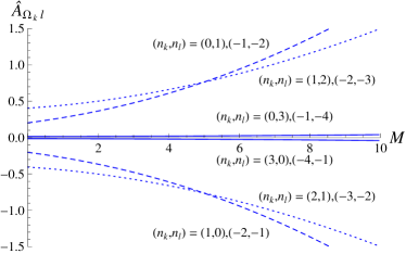
(a) (b)

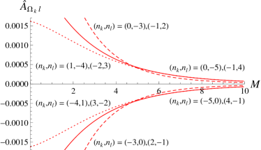
Figure 2: Behaviour of the Bogoliubov coefficients for the massive $(1+1)$-dimensional Dirac field with MIT bag boundary conditions for increasing mass. The coefficient of $h$ in (VI.23), denoted by $\hat{A}_{\Omega_{k}l}(M)$, is plotted against the dimensionless combination $M:={\mu}L$. Figure 2 (a) shows a selection of Bogoliubov coefficients that relate modes with the same sign of the frequency ($\alpha$-type coefficients): the map $k\mapsto n_{k}$ has been chosen so that $n_{k}\geq 0$ labels the positive frequency solutions and $n_{k}<0$ labels the negative frequency solutions. These mode-mixing coefficients are proportional to $M^{2}$ as $M\rightarrow\infty\,$. Figure 2 (b) shows a selection of Bogoliubov coefficients that relate positive frequency modes with negative frequency modes ($\beta$-type coefficients). These particle creation coefficients are proportional to $M^{-6}$ as $M\rightarrow\infty\,$.

In scenarios where entanglement generation between two or more modes in a single cavity is considered, the leading-order effects are determined by the coefficients of $h$ in (VI.23) Friis:2011yd . As noted above, we denote these coefficients by $\hat{A}_{\Omega_{k}l}(M)$, indicating explicitly their dependence on ${\mu}$ and $L$ through the dimensionless combination $M:={\mu}L$. Selected plots are shown in Fig. 2. In the limit $M\to\infty$, it can be shown from (VI.23) that the mode-mixing coefficients increase proportionally to $M^{2}$ [Figure 2 (a)], while the particle-creation coefficients decrease proportionally to $M^{-6}$ [Figure 2 (b)]. The relevance of this behaviour becomes apparent when we consider initial pure states of two modes labelled by $n_{k}$ and $n_{k^{\prime}}$, respectively. The coefficient $\hat{A}_{\Omega_{k}k^{\prime}}$ is directly related to the entanglement that is created between these modes due to the cavity motion Friis:2012tb . The qualitatively different dependence on the field mass for mode-mixing and particle-creation Bogoliubov coefficients indicates that nonzero mass enhances entanglement generation between modes of equal charge, while the effect is suppressed between modes of opposite charge.

Finally, it is also of interest to reconsider the massless limit. As noted before, the coefficients for the MIT bag boundary condition reduce to the case $s=\tfrac{1}{2}$ (rather than $s=0$) discussed in Friis:2011yd . Since this choice removes the zero mode from the spectrum, the resulting Bogoliubov coefficients allow for a violation of the Clauser-Horne-Shimony-Holt inequality ClauserHorneShimonyHolt1969 ; HorodeckiRPM1995 by the entanglement generated from the initial vacuum state.

VII Unitarity of evolution

In this section we address the unitary implementability of the cavity field’s time evolution, for both smoothly varying and sharply varying accelerations. We treat the boson fields and the spinor field in turn.

VII.1 Bosons

Recall that a Bogoliubov transformation for a real bosonic field, with the coefficient matrices written in our notation as $\alpha=(\alpha_{ij})$ and $\beta=(\beta_{ij})$ byd , is implementable as a unitary transformation iff the matrix $\alpha^{-1}\beta$ is Hilbert-Schmidt, $\sum_{ij}{|(\alpha^{-1}\beta)_{ij}|}^{2}<\infty$ shale-unitarity ; shale-stinespring ; honegger-rieckers ; labonte .

We start with the $(1+1)$-dimensional scalar field of Secs. II and III, and with the Bogoliubov transformation from the inertial segment to the uniformly accelerated segment. While the perturbative small acceleration expansions of the Bogoliubov coefficients in (II.12) and (III.3) are not uniform in the mode numbers, we may nevertheless examine the unitarity of the dynamics perturbatively in $h$. To leading order in $h$, this reduces to considering the linear terms in (II.12) and (III.3), and to this order the Hilbert-Schmidt condition for ${{}_{\text{o}}\alpha}^{-1}{{}_{\text{o}}\beta}$ is equivalent to the Hilbert-Schmidt condition for ${{}_{\text{o}}\beta}$.

In the notation established in Secs. II and III, we denote the coefficient of $h$ in the expansion of ${{}_{\text{o}}\beta}_{mn}$ in (II.12c) or (III.3c) by $\hat{\beta}_{mn}(M)$, continuing to suppress the distinction between Dirichlet and Neumann, but indicating explicitly the dependence on ${\mu}$ and $L$ through the dimensionless combination $M:={\mu}L$. Elementary estimates show that the function $F(M):=\sum_{mn}\bigl{|}\hat{\beta}_{mn}(M)\bigr{|}^{2}$ is finite for all values of $M$. The field evolution in the sharp transition from the inertial segment to the uniformly accelerated segment is hence perturbatively unitary to linear order in $h$.

Suppose then that the acceleration varies smoothly between an initial inertial region and a final inertial region, so that to linear order in the acceleration the Bogoliubov coefficients are given by (II.14), where $\hat{\alpha}_{mn}(M)$ and $\hat{\beta}_{mn}(M)$ are the coefficients of $h$ in the expansions of ${{}_{\text{o}}\alpha}_{mn}$ and ${{}_{\text{o}}\beta}_{mn}$ (II.12) or (III.3). As the Fourier transform of a smooth function of compact support falls off at infinity faster than any power, (II.14c) shows that ${{}_{\text{s}}\beta}_{mn}$ is bounded in absolute value by $\bigl{|}\hat{\beta}_{mn}(M)f(\omega_{m}+\omega_{n})\bigr{|}$, where $f$ is a function that falls off at infinity faster than any power. The sum $\sum_{mn}\bigl{|}{{}_{\text{s}}\beta}_{mn}\bigr{|}^{2}$ is hence finite. We conclude that the evolution is perturbatively unitary to linear order in the acceleration.

Consider then a rectangular cavity in a higher-dimensional spacetime, with acceleration in one of its principal directions. By Fourier decomposition in the transverse dimensions, the Bogoliubov transformation reduces to that of the $(1+1)$-dimensional cavity for each set of the transverse quantum numbers, with the transverse momenta contributing to the effective $(1+1)$-dimensional mass. The trace in the Hilbert-Schmidt norm includes now also a sum over the transverse quantum numbers. For the sharp evolution from inertial motion to uniform acceleration, the criterion of leading-order perturbative unitarity is hence the finiteness of the sum $\sum_{\mathbf{k}_{\perp}}F(L\sqrt{\mu_{0}^{2}+\mathbf{k}^{2}_{\perp}})$, where $\mu_{0}$ is the genuine mass and $\mathbf{k}_{\perp}$ are the quantised transverse momenta. It follows from the estimates given in the Appendix that this criterion is satisfied in $(2+1)$ dimensions but not in $(3+1)$ or higher. The perturbative unitarity of the dynamics hence fails in $(3+1)$ spacetime dimensions and above when the onset of the acceleration is sharp. When the acceleration changes smoothly, by contrast, the rapid falloff of $\sum_{mn}\bigl{|}{{}_{\text{s}}\beta}_{mn}\bigr{|}^{2}$ guarantees that the evolution is unitary in any spacetime dimension.

Finally, as the Maxwell field in a $(3+1)$-dimensional cavity decomposes into Dirichlet-type polarisation modes and Neumann-type polarisation modes, the results about the perturbative unitarity of the time evolution follow directly from those for the scalar field. Unitarity holds when the acceleration changes smoothly but fails when the acceleration onset is sharp.

VII.2 Fermions

For a fermionic field, a Bogoliubov transformation is unitarily implementable if the two blocks of the Bogoliubov transformation matrix that relate positive frequencies to negative frequencies are Hilbert-Schmidt thaller:dirac ; shale-unitarity ; shale-stinespring ; honegger-rieckers ; labonte . We consider this condition in our system perturbatively in the acceleration, to the leading order.

Consider first the $(1+1)$-dimensional Dirac field of Section VI and the Bogoliubov transformation from the inertial segment to the uniformly accelerated segment. Recall that we denote the coefficient of $h$ in (VI.23) by $\hat{A}_{\Omega_{k}l}(M)$, indicating explicitly the dependence on ${\mu}$ and $L$ through the dimensionless combination $M:={\mu}L$. The condition of unitarily implementable evolution for given $M$ is then that $G(M):=\sum_{k>0>l}\bigl{|}\hat{A}_{\Omega_{k}l}(M)\bigr{|}^{2}$, or equivalently $G(M):=\sum_{l>0>k}\bigl{|}\hat{A}_{\Omega_{k}l}(M)\bigr{|}^{2}$, is finite. Elementary estimates show that this condition holds for all $M$.

When the acceleration varies smoothly in time, the Bogoliubov coefficient matrix between an initial inertial region and a final inertial region is given by (VI.25). The rapid falloff of the Fourier transform guarantees that the unitarity condition is satisfied.

Consider then a rectangular cavity in a higher-dimensional spacetime, with acceleration in one of its principal directions. Proceeding as for the scalar field, and using the large $M$ behaviour of $G(M)$ established in the Appendix, we find that the situation is as for the scalar field: unitarity holds for smoothly varying acceleration in any spacetime dimension but fails for sharply varying acceleration in spacetime dimension $(3+1)$ and higher.

VIII Conclusions

In this paper we have investigated scalar, spinor, and photon fields in a cavity that is accelerated in Minkowki spacetime. The cavity was assumed mechanically rigid, and we worked within a recently introduced perturbative formalism Bruschi:2011ug that assumes accelerations to remain small compared with the inverse linear dimensions of the cavity but allows the velocities, travel times, and travel distances to be arbitrary, and in particular includes the regime where the velocities are relativistic. We extended previous scalar field analyses to cover both Dirichlet and Neumann boundary conditions, and we showed that a photon field in $(3+1)$ spacetime dimensions with perfect conductor boundary conditions decomposes into Dirchlet-type and Neumann-type polarisation modes. For a Dirac spinor, we extended previous work on $(1+1)$-dimensional massless spinors to a strictly positive $(1+1)$-dimensional mass: this is necessary to handle a cavity in dimensions higher than $(1+1)$, where the dimensions transverse to the acceleration give a strictly positive contribution to the effective $(1+1)$-dimensional mass. We also presented the spinor field time evolution formulas for acceleration with arbitrary time dependence, in parallel with the scalar field formulas given in Bruschi:2012pd . We discussed briefly the consequences of the nonvanishing $(1+1)$-dimensional mass for quantum information tasks with Dirac fermions, noting that the mass and the absence of a zero mode can enhance both entanglement degradation and generation effects.

Finally, we considered whether particle creation in the cavity could become strong enough to prevent the time evolution of the quantum field from being implementable as a unitary transformation in the Fock space. Working to linear order in the acceleration, we found the evolution to be unitary when the acceleration varies smoothly in time. In the limit of discontinously varying accelerations the evolution remains unitary in spacetime dimensions $(1+1)$ and $(2+1)$ but becomes nonunitary in spacetime dimensions $(3+1)$ and higher.

While the focus of this paper was theoretical, we shall finish by recalling two experimental situations for which our results are relevant.

First, traditional proposals to observe acceleration effects in the laboratory use photons moore-dyncas ; Reynaud1 ; Dodonov:advchemphys ; Dodonov:2010zza , and success in observing the generated photons has been recently reported in an experiment where acceleration is simulated by SQUID circuits wilson-etal . Our results confirm that the small acceleration cavity formalism that was introduced in Bruschi:2011ug for a scalar field adapts in a straightforward way to the electromagnetic field. It follows in particular that the experimental scenario of mode mixing in a cavity accelerated on a desktop, proposed and analysed for a scalar field in Bruschi:2012pd , does apply to photons captured in the cavity.

Second, it has been proposed that acceleration effects for fermions can be simulated in solid state analogue systems boada:dirac ; ZhangWangZhu2012 ; Iorio2012 . Our work provides the theoretical framework for analysing such acceleration effects with cavitylike boundary conditions whenever the fermion field has a mass and/or dimensions transverse to the acceleration.

Appendix A Asymptotics of Bogoliubov coefficient sums

In this Appendix we establish the asymptotic large $M$ behaviour of the functions $F(M)$ and $G(M)$ defined in Sec. VII.

Recall that $F(M):=\sum_{mn}\bigl{|}\hat{\beta}_{mn}(M)\bigr{|}^{2}$, where $\hat{\beta}_{mn}(M)$ is the coefficient of $h$ in the expansion of ${{}_{\text{o}}\beta}_{mn}$ in (II.12c) or (III.3c), where the notation suppresses the distinction between the Dirichlet and Neumann boundary conditions but indicates explicitly the dependence on ${\mu}$ and $L$ through the dimensionless combination $M:={\mu}L>0$. Recall similarly that $G(M):=\sum_{k>0>l}\bigl{|}\hat{A}_{\Omega_{k}l}(M)\bigr{|}^{2}$, or equivalently $G(M):=\sum_{l>0>k}\bigl{|}\hat{A}_{\Omega_{k}l}(M)\bigr{|}^{2}$, where $\hat{A}_{\Omega_{k}l}(M)$ is the coefficient of $h$ in (VI.23).

Elementary estimates show that $F(M)$ and $G(M)$ are finite for all $M$. At $M\to\infty$, we find

$$\begin{aligned} M^{2}F(M)\to\begin{cases}\displaystyle\frac{2}{\pi^{2}}\int\limits_{\begin{subarray}{c}x>0\\ y>0\end{subarray}}\frac{x^{2}y^{2}\,dx\,dy}{\sqrt{1+x^{2}}\sqrt{1+y^{2}}\,\bigl{(}\sqrt{1+x^{2}}+\sqrt{1+y^{2}}\,\bigr{)}^{6}}\ =\frac{1}{90\pi^{2}}\ ,&\text{(Dirichlet)}\\[21.52771pt] \displaystyle\frac{2}{\pi^{2}}\int\limits_{\begin{subarray}{c}x>0\\ y>0\end{subarray}}\frac{\bigl{(}\sqrt{1+x^{2}}\sqrt{1+y^{2}}\,+1\bigr{)}^{2}\,dx\,dy}{\sqrt{1+x^{2}}\sqrt{1+y^{2}}\,\bigl{(}\sqrt{1+x^{2}}+\sqrt{1+y^{2}}\,\bigr{)}^{6}}\ =\frac{11}{90\pi^{2}}\ ,&\text{(Neumann)}\end{cases}\end{aligned}$$ (A.1a)

$$\begin{aligned} M^{2}G(M)&\to\frac{8}{\pi^{2}}\mathop{{\int}}\limits_{\begin{subarray}{c}x>0\\ y>0\end{subarray}}\frac{\bigl{(}\sqrt{1+x^{2}}+x-\sqrt{1+y^{2}}-y\bigr{)}^{2}\bigl{[}\bigl{(}\sqrt{1+x^{2}}+x\bigr{)}\bigl{(}\sqrt{1+y^{2}}+y\bigr{)}-1\bigr{]}^{2}}{\bigl{(}\sqrt{1+x^{2}}+x+\sqrt{1+y^{2}}+y\bigr{)}^{6}\bigl{[}\bigl{(}\sqrt{1+x^{2}}+x\bigr{)}\bigl{(}\sqrt{1+y^{2}}+y\bigr{)}+1\bigr{]}^{6}}\\[4.30554pt] &\hskip 43.05542pt\times\frac{x^{2}y^{2}\,\bigl{(}\sqrt{1+x^{2}}+x\bigr{)}^{4}\bigl{(}\sqrt{1+y^{2}}+y\bigr{)}^{4}}{(1+x^{2})(1+y^{2})}\>dx\,dy\ ,\\[4.30554pt] &\hskip 12.91663pt=\frac{7}{45\pi^{2}}-\frac{1}{64}\ ,\end{aligned}$$ (A.1b)

where the integral expressions ensue by regarding the sum as a Riemann sum: in (A.1a) we have set $x=(\pi/M)m$ and $y=(\pi/M)n$, and in (A.1b) we have set $x=|k|/{\mu}$ and $y=|l|/{\mu}$. The integrals can be evaluated by the substitution $x=\tfrac{1}{2}(u-u^{-1})$, $y=\tfrac{1}{2}(v-v^{-1})$.

References

- (1) S. W. Hawking, Commun. Math. Phys. 43, 199 (1975); ibid. 46, 206(E) (1976)].
- (2) W. G. Unruh, Phys. Rev. D 14, 870 (1976).
- (3) L. C. B. Crispino, A. Higuchi, and G. E. A. Matsas, Rev. Mod. Phys. 80, 787 (2008) .
- (4) G. T. Moore, J. Math. Phys. 11, 2679 (1970).
- (5) A. Lambrecht, M.-T. Jaekel, and S. Reynaud, Phys. Rev. Lett. 77, 615 (1996).
- (6) V. V. Dodonov, Adv. Chem. Phys. 119, 309 (2001).
- (7) V. V. Dodonov, Phys. Scripta 82, 038105 (2010).
- (8) L. Parker, Phys. Rev. 183, 1057 (1969).
- (9) L. Parker, Phys. Rev. D 3, 346 (1971).
- (10) C. Barceló, S. Liberati, and M. Visser, Living Rev. Rel- ativity 8, 12 (2005).
- (11) D. Rideout, T. Jennewein, G. Amelino-Camelia, T. F. Demarie, B. L. Higgins, A. Kempf, A. Kent, R. Laflamme, X. Ma, R. B. Mann, E. Martín-Martínez, N. C. Menicucci, J. Moffat, C. Simon, R. Sorkin, L. Smolin, and D. R. Terno, Classical Quantum Gravity 29, 224011 (2012), Focus Issue on ‘Relativistic Quantum Information’.
- (12) D. E. Bruschi, I. Fuentes, and J. Louko, Phys. Rev. D 85, 061701(R) (2012).
- (13) D. E. Bruschi, J. Louko, D. Faccio, and I. Fuentes, New J. Phys. 15, 073052 (2013).
- (14) D. E. Bruschi, J. Louko, and D. Faccio, J. Phys.: Conf. Ser. 442, 012024 (2013).
- (15) D. A. R. Dalvit and F. D. Mazzitelli, Phys. Rev. A 59, 3049 (1999).
- (16) D. T. Alves, E. R. Granhen, and W. P. Pires, Phys. Rev. D 82, 045028 (2010).
- (17) N. Friis, A. R. Lee, D. E. Bruschi, and J. Louko, Phys. Rev. D 85, 025012 (2012).
- (18) N. Friis, D. E. Bruschi, J. Louko, and I. Fuentes, Phys. Rev. D 85, 081701(R) (2012).
- (19) D. E. Bruschi, A. Dragan, A. R. Lee, I. Fuentes, and J. Louko, Phys. Rev. Lett. 111, 090504 (2013).
- (20) P. M. Alsing and I. Fuentes, Classical Quantum Gravity 29, 224001 (2012), Focus Issue on ‘Relativistic Quantum Information’.
- (21) N. Friis, M. Huber, I. Fuentes, and D. E. Bruschi, Phys. Rev. D 86, 105003 (2012).
- (22) N. Friis and I. Fuentes, J. Mod. Opt. 60, 22 (2013).
- (23) N. Friis, A. R. Lee, K. Truong, C. Sabín, E. Solano, G. Johansson, and I. Fuentes, Phys. Rev. Lett. 110, 113602 (2013).
- (24) C. M. Wilson, G. Johansson, A. Pourkabirian, M. Simoen, J. R. Johansson, T. Duty, F. Nori, and P. Delsing, Nature (London) 479, 376 (2011).
- (25) O. Boada, A. Celi, J. I. Latorre, and M. Lewenstein, New J. Phys. 13, 035002 (2011).
- (26) D.-W. Zhang, Z.-D. Wang, and S.-L. Zhu, Front. Phys. 7, 31 (2012).
- (27) A. Iorio, Eur. Phys. J. Plus 127, 156 (2012).
- (28) A. Chodos, R. L. Jaffe, K. Johnson, C. B. Thorn, and V. F. Weisskopf, Phys. Rev. D 9, 3471 (1974).
- (29) E. Elizalde, M. Bordag, and K. Kirsten, J. Phys. A: Math. Gen. 31, 1743 (1998).
- (30) N. D. Birrell and P. C. W. Davies, Quantum Fields in Curved Space (Cambridge University Press, Cambridge, England, 1982).
- (31) S. Takagi, Prog. Theor. Phys. Suppl. 88, 1 (1986).
- (32) NIST Digital Library of Mathematical Functions, http://dlmf.nist.gov/, release 1.0.6 of 2013-05-06.
- (33) T. M. Dunster, SIAM J. Math. Anal. 21, 995 (1990).
- (34) T.-M. Zhao and R.-X. Miao, Opt. Lett. 36, 4467 (2011).
- (35) J. D. Jackson, Classical Electrodynamics (Wiley, New York, 1999), 3rd edition.
- (36) P. A. M. Dirac, Lectures on Quantum Mechanics (Dover, New York, 2003).
- (37) M. Henneaux and C. Teitelboim, Quantization of Gauge Systems (Princeton University Press, Princeton, 1992).
- (38) L. H. Ford and T. A. Roman, Ann. Phys. (N. Y.) 326, 2294 (2011).
- (39) M. Srednicki, Quantum Field Theory (Cambridge University Press, Cambridge, England, 2007).
- (40) M. Reed and M. Simon, Methods of Modern Mathematical Physics (Academic Press, New York, 1975), Vol. 2.
- (41) G. Bonneau, J. Faraut, and G. Valent, Am. J. Phys. 69, 322 (2001).
- (42) B. Thaller, The Dirac Equation (Springer, Berlin, 1992).
- (43) B. Belchev and M. A. Walton, J. Phys. A 43, 085301 (2010).
- (44) D. McMahon, P. M. Alsing, and P. Embid, eprint arXiv:gr-qc/0601010 (2006).
- (45) P. Langlois, Phys. Rev. D 70, 104008 (2004); ibid. D 72, 129902(E) (2005)].
- (46) P. Langlois, Ph.D. thesis, University of Nottingham (2005) [arXiv:gr-qc/0510127].
- (47) F. W. J. Olver, Philos. Trans. Roy. Soc. London. Ser. A. 247, 328 (1954).
- (48) N. Friis, A. R. Lee, and D. E. Bruschi, Phys. Rev. A 87, 022338 (2013).
- (49) J. F. Clauser, M. A. Horne, A. Shimony, and R. A. Holt, Phys. Rev. Lett. 23, 880 (1969).
- (50) M. Horodecki, P. Horodecki, and R. Horodecki, Phys. Lett. A 200, 340 (1995).
- (51) D. Shale, Trans. Am. Math. Soc. 103, 149 (1962).
- (52) D. Shale and W. F. Stinespring, Indiana Univ. Math. J. (formerly: J. Math. Mech.) 14, 315 (1965).
- (53) R. Honegger and A. Rieckers, J. Math. Phys. 37, 4292 (1996).
- (54) G. Labonté, Commun. Math. Phys. 36, 59 (1974).