iint TXFiint

A general, efficient and robust method for calculating free energy difference between systems

Calculating free energy differences is a topic of substantial interest and has many applications including chemical reactions, molecular docking and hydration, solvation and binding free energies which are used in computational drug discovery. However, in the existing practices in relative free energy calculations the implementation is rather complicated, the simulated hybrid system can suffer from small phase space overlap and there remain the challenges of robustness and automation. Here an efficient and robust method, that enables a wide range of comparisons, will be introduced, demonstrated and compared. In this method instead of artificially transforming one system into the other to perform the calculation, each system is transformed into its replica with the different long range energy terms relaxed, which is inherently correlated with the original one, in order to eliminate the partition function difference arising from these terms. Then, since each transformed system can be treated as non interacting systems, the remaining difference in the (originally highly complex) partition function will cancel out.

Calculating free energy differences between two physical systems, is a topic of substantial current interest. A variety of advanced methods and algorithms have been introduced to answer the challenge, both in the context of Molecular Dynamics and Monte Carlo simulations [1, 2, 3, 4, 5]. Applications of these methods include calculations of binding free energies [6, 7, 8], free energies of hydration [9], free energies of solvation [10], transfer of a molecule from gas to solvent [4], chemical reactions [11] and more. Binding free energy calculations are of high importance since they can be used for molecular docking [12] and in drug discovery[13]. Free energy methods are extensively used by various disciplines and the interest in this field is growing - over 3,500 papers using the most popular free energy computation approaches were published in the last decade, with the publication rate increasing $\sim 17\%$ per year [14].

Free energy difference between two systems can be calculated using equilibrium methods (alchemical free energy calculations) and non equilibrium methods. In equilibrium methods a hybrid system is used to transform system $A$ into $B$, usually with the transformation $H_{\_}{hybrid}=\lambda H_{\_}{A}+\left(1-\lambda\right)H_{\_}{B},\,\lambda=[0,1]$ . In these methods, first the intermediates ($\lambda$s) that interpolate between the systems are selected and the hybrid system is simulated at these intermediates and average values are calculated. Then, using these values, the free energy difference is calculated. The commonly used methods include Bennett Acceptance Ratio [15], Weighted Histogram Analysis Method [16], Exponential Averaging/ Free Energy Perturbation [17] and Thermodynamic Integration (ThI) [3, 18, 19]. In non equilibrium methods the work needed in the process of switching between the two Hamiltonians is measured. These methods include Jarzynski relation [20] (fast growth is one of its applications [21]) and its subsequent generalization by Crooks [22]. Most of the applications mentioned above can be tackled from a different direction using methods which measure the free energy as a function of a reaction coordinate. These methods include Adaptive Biasing Force [23] and Potential Mean Force [18] (fast growth also belongs to this type of methods).

Calculating binding free energies is fundamental and has many applications. In particular it has potential to advance the field of drug discovery which has to cope with new challenges. In the last years the number of innovative new molecular entities (for pharmaceutical purposes) has remained stable at $5-6$ per year. This situation is especially grim when taking into account the continual emergence of drug-resistant strains of viruses and bacteria. Virtual screening methods, in which the $10^{60}$ possible molecules are filtered out, play a large role in modern drug discovery efforts. However, there remains the challenge of selecting the candidate molecules out of the still very large pool of molecules in reasonable times. Equilibrium methods show great potential in enabling the computation of binding free energies with reasonable computational resources. In these methods instead of simulating the binding processes directly, which would require a simulation many times the lifetime of the complex, the ligand is transmuted into another through intermediate, possibly nonphysical stages [14]. Then if the free energy difference between the ligands in the two environments are calculated [24], the binding free energy difference between the two ligands can be calculated (this cyclic calculation is called the Thermodynamic Cycle).

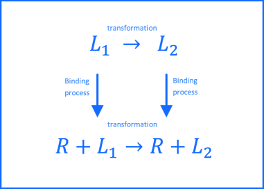
Figure 1: Scheme of the free energy differences in the calculation of binding free energy in the existing methods

In Fig 1 a scheme of the free energies in the calculation of binding free energies in the existing methods is presented ($L_{\_}1,L_{\_}2$ and $R$ represent the ligands and receptor respectively).

Free energy calculation methods already have successes in discovering potent drugs[13]. However, despite the continuing progress in the field from the original concepts, the methods have restrictions which prevent them from being automatic and limit their use in computational drug design [14]. A naive calculation of the free energy difference using ThI can be performed as follows:

$$\triangle F_{\_}{A\rightarrow B}\left(\beta_{\_}{1}\right)=\int_{\_}0^{1}\frac{dF_{\_}{A\rightarrow B}\left(H_{\_}{hybrid}\left(\lambda\right)\right)}{d\lambda}d\lambda=$$ (1)

$$\int_{\_}0^{1}\int\frac{\left[H_{\_}{B}(\Omega)-H_{\_}{A}(\Omega)\right]e^{-\beta_{\_}{1}\left[\lambda H_{\_}{B}(\Omega)+\left(1-\lambda\right)H_{\_}{A}(\Omega)\right]}d\Omega}{Z(\lambda)}d\lambda$$ (2)

It can be seen that at $\lambda=1$ for example $H_{\_}{A}$ does not affect the systems’ behavior but its energy values are averaged over, which can result in large magnitudes of the integrated function. Thus, when the systems have low phase space overlap there are significant changes in the integrated function and large variance and hence large computational cost. This is especially dominant when the systems have different covalent bond description which results in a very low phase space overlap. Many approaches and techniques have been introduced to address the challenges in the field. These include the topologies for simulating the hybrid system (single and dual topology), soft core potentials, the notion of decoupling atoms and more. Common sampling techniques to overcome energy barriers include Temperature and Hamiltonian Replica Exchange methods. However, the implementation of equilibrium methods is notoriously difficult to implement correctly [25]. Such complications arise for example from the fact that in the hybrid system there is one set of coordinates that describes both systems simultaneously and hence the hybrid system usually has to be designed. In addition each type of topology has small phase space overlap in one aspect [pearlman1994comparison]. Also, since both systems interact simultaneously with the environment the behavior of the intermediate systems cannot be predicted. Moreover, since the process of transforming one system into the other is non physical and different for each comparison, the choice of intermediates for the hybrid system remains a challenge.

Temperature Integration (TeI) was suggested in [26] as an efficient method to calculate free energy differences. While TeI has many advantages it cannot be directly applied to molecular simulations in which bond stretching is allowed and to Molecular Dynamics. This is since the use of the capping in the covalent bond terms (denoted as $E_{\_}{cap}$ in TeI ) will result in a phase transition which will result in impractical simulations in the canonical ensemble and since MD simulations at very high temperatures (suggested in TeI) are impractical due to the very high velocities. In addition, the phase space overlap between the compared systems is rather low since, effectively, all the energy terms are relaxed. Here, based on TeI, a general method that solves these three challenges will be presented. This method also addresses the current challanges in the field that were stated before.

The method was derived from principles of statistical physics, independently of the methodology in the field mentioned above. In section the method will be introduced in a logical developmental order and will be linked in places of similarity to the relevant literature. In section the derivation will be put in context of the methodology in the field and will be divided into its ingredients. This section is also aimed for practitioners that are interested in the decription of the method in the terminology of the field (the article is thus aimed both for physicists and practitioners). As will become clear, the independent ingredients of the method are: a different approach to topology with a relevant sampling technique, unified approach to soft core potentials and a minor improvement in the decoupling scheme. It is emphasized that the main ingredient of the method is that instead of simulating a hybrid system, two separate systems are simulated (related to topology).

The method

The idea is to transform the systems $A$ and $B$ (between which the free energy difference is calculated) into two systems that have the same partition function up to factors that can be calculated. In the transformation the energy terms are lowered (or unchanged) and as a result the corresponding partition functions value will change monotonously, which will enable a simple selection of intermediates for the calculation of free energy difference. In this process in case there are covalent bonds terms (represented by harmonic potential), their strength will stay constant in order to avoid phase transition (molecular modeling includes covalent bond, bond angle, dihedral angle, electric and VDW potentials [27, 28]). For the systems $A$,$B$ the following Hamiltonians as a function of $\lambda$ are defined:

$$H_{\_}{A/B}\left(\lambda\right)=\lambda H_{\_}{{}_{\_}{{A_{\_}{nc}/B_{\_}{nc}}}}+H_{\_}{{}{A_{\_}c/B_{\_}c}}$$ (3)

where $H_{\_}{{}_{\_}{{A_{\_}{nc}/B_{\_}{nc}}}}$ denote the non covalent potential terms and $H{{}_{\_}{A_{\_}{c}/B_{\_}{c}}}$ denote the covalent bond terms, with the corresponding partition functions:

$$\tilde{Z}_{\_}{A/B}\left(\lambda\right)=\int e^{-\beta\left(\lambda H_{\_}{{}_{\_}{{A_{\_}{nc}/B{nc}}}}+H_{\_}{{A_{\_}c/B_{\_}c}}\right)}d\Omega$$ (4)

It has to be noted that the integration over momentum is not presented since it yields known terms and can be factored out.

Since even at $\lambda\rightarrow 0$ the energy terms that diverge at $r=0$ are still dominant and cause a difference between the partition functions of the two systems, capping is used in the non covalent terms (if $E>E_{\_}{cap}$ $E=E_{\_}{cap}$). Thus, the partition functions at $\lambda\rightarrow 0$ are equal up to factors that originate from the covalent bonds that are different. The proposed calculation of the free energy difference between the two systems is legitimate only if the choice of the capping energy has a negligible effect on the partition function value of each of the two systems at $\lambda=1$. The Hamiltonian with the capping in all the non covalent energy terms denoted by $H^{\prime}$ is written as follows:

$$H^{\prime}_{\_}{A/B}\left(\beta,\lambda\right)=\lambda H^{\prime}_{\_}{{}_{\_}{{A_{\_}{nc}/B_{\_}{nc}}}}+H_{\_}{{}{A_{\_}c/B_{\_}c}}$$ (5)

The requirement stated above can be written explicitly as follows:

$$ln\tilde{Z}_{\_}{A/B}\left(\beta,\lambda=1,H^{\prime}\right)\backsimeq ln\tilde{Z}_{\_}{A/B}\left(\beta,\lambda=1,H\right)$$ (6)

It can be seen that at $\lambda=0$:

$$ln\tilde{Z}_{\_}{A}\left(\beta,\lambda=0,H^{\prime}\right)-ln\tilde{Z}_{\_}{B}\left(\beta,\lambda=0,H^{\prime}\right)=\\$$ (7)

$$\Delta ln\tilde{Z}_{\_}{{A_{\_}c\rightarrow B_{\_}c}}\left(\beta,0,H^{\prime}\right)$$ (8)

where $ln\tilde{Z}_{\_}{A_{\_}{c}/B_{\_}{c}}\left(\beta,\lambda=0,H^{\prime}\right)$ are defined as follows:

$$\tilde{Z}_{\_}{A_{\_}{c}/B_{\_}{c}}\left(\beta,\lambda=0,H^{\prime}\right)=\int e^{-\beta H_{\_}{A_{\_}{c}/B_{\_}{c}}}d\Omega$$ (9)

In order for the capping to have a negligible effect on the partition functions at $\lambda=1$ it has to be set to a value that satisfies:

$$e^{-\frac{E_{\_}{cap}}{kT}}\ll 1$$ (10)

Thus at $\lambda$ values satisfying $e^{-\frac{\lambda E_{\_}{cap}}{kT}}\ll 1$ the corresponding interactions, including the steric, become transparent [24]. It is noted that the capping has a negligible effect on the partition function of realistic molecular systems independently of the atom pairs. This is since each atom has an average potential energy of typical value of $k_{\_}{B}T$ above the average energy (the capping energy can be set relative to the the average pair total long range energy) and since the denisty of states for $E>E_{\_}{cap}$ is very low (dual effect). It has been shown in the context of MC that there is a tradeoff when choosing $E_{\_}{cap}$ (behavior of the function vs. accuracy) [29] and that values of $\leavevmode\nobreak\ 5$kCal/mol [29] enable accurate free energy calculations. The fact that the force is zero in some of the range is legitimate in MD simulations since the particles have thermal velocities and they are affected by other potentials (also there exist other potentials without force at certain distances e.g the VdW and the Coulomb potentials at large distances). It is noted that a switching function between the standard long range potential and the flat potential is needed in order have continuity in the derivative that will enable the integration over the equations of motion in MD to be valid. This has been developed independently and implemented in MD with a cubic switching function and an energetically inaccessible capping which validates its use in the context of MD for high energetic values [31]. Thus a unified approach is suggested that uses quadratic switching function and capping energy that is accessible and has a negligible effect on the free energy as a soft core technique.

From here on $H^{\prime}$ will be used in all the $\tilde{Z}$ terms:

$$\tilde{Z}_{\_}{A/B}\left(\beta,\lambda\right)\triangleq\tilde{Z}_{\_}{A/B}\left(\beta,\lambda,H^{\prime}\right)$$ (11)

When the systems have the same degrees of freedom the free energy difference can be written as follows:

$$F_{\_}{A\rightarrow B}(\beta)=-k_{\_}BT\left[\ln{Z_{\_}B(\beta)}-\ln{Z_{\_}A(\beta)}\right]\backsimeq\\$$

$$-k_{\_}BT\big{[}\ln{\tilde{Z}_{\_}B(\beta,1)}-\ln{\tilde{Z}_{\_}B(\beta,0)}+\ln{\tilde{Z}_{\_}A(\beta,0)}\\$$

$$\Delta\ln{\tilde{Z}_{\_}{{B_{\_}c\rightarrow A_{\_}c}}(\beta,0)}-\ln{\tilde{Z}_{\_}A(\beta,1)}\big{]}=\\$$

$$\int_{\_}0^{1}\langle H^{\prime}_{\_}{B_{\_}{nc}}\rangle d\lambda-\int_{\_}0^{1}\langle H^{\prime}_{\_}{A_{\_}{nc}}\rangle d\lambda-k_{\_}BT\Delta\ln{\tilde{Z}_{\_}{{B_{\_}c\rightarrow A_{\_}c}}(\beta,0)}$$ (12)

using equations (6), the earlier definition of $\Delta ln\tilde{Z}_{\_}{{B_{\_}c\rightarrow A_{\_}c}}\left(\beta,0\right)$ and the following identity:

$$\ln\tilde{Z}_{\_}{A/B}\left(\beta,1\right)-ln\tilde{Z}_{\_}{A/B}\left(\beta,0\right)=\int_{\_}0^{1}\frac{dln\tilde{Z}_{\_}{A/B}\left(\beta,\lambda\right)}{d\lambda}d\lambda\\$$ (13)

Assuming the factor $\Delta ln\tilde{Z}_{\_}{B_{\_}{c}\rightarrow A_{\_}{c}}\left(\beta,0\right)$, that can be different than zero just in molecular simulations in which bond stretching is allowed, is known, the calculation of the free energy difference can thus be performed. Thus, the systems are simulated at the same temperature and the molecule stays in its covalently bounded state (which enables MD simulations that are not practical at very high temperatures due to the short time steps needed and modelling that includes bond strecthing respectively).

When the systems, between which the free energy difference is calculated, have rugged energy landscape, one can use techniques such as H-REMD/H-PT (Hamiltonian Replica Exchange MD/ Hamiltonian Parallel Tempering, variant of Parallel Tempering/Replica Exchange [32, 33, 34]) to alleviate sampling problems [35]. In this technique the system is simulated at a set of $\lambda$s and exchanges of configurations between them are performed every certain number of steps. Thus, the systems at the low $\lambda$s, that can cross energetic barriers, help the system of interest to be sampled well. This technique, even though is highly efficient, introduces another dimension of sampling since simulations of replicas of the system at a set of $\lambda$s are performed at each intermediate of the hybrid system (sampling the dimensions of $\lambda$ that interpolates between the systems and of $\lambda$ of the replicas that are used for the equilibration). Here, the simulations at the different $\lambda$s will be used also to calculate the free energy difference by integration and the need for another sampling dimension is eliminated.

It has to be mentioned that the less energy terms are multiplied by $\lambda$, the more correlated the systems at $\lambda=0$ and at $\lambda=1$ are, resulting in a much shorter calculation. In particular, keeping the dihedral and bonding angles terms constant can result in less intermediates and shorten the simulation time even more. Thus the energy terms can be separated into short range (covalent bond, bond angle, dihedral angle and improper dihedral angle) and long range (electric and VDW). In the existing practices they are called bonded interactions and non bonded interactions and it was decided to use these names in order to emphasize the fact that the potentials link up to 3rd nearest neighbor and all atoms respectively which have implication later on. The Hamiltonians can be written as follows:

$$H^{\prime}_{\_}{A/B}\left(\lambda\right)=\lambda H^{\prime}_{\_}{{}_{\_}{{A_{\_}{lr}/B_{\_}{lr}}}}+H_{\_}{{}{A_{\_}{sr}/B_{\_}{sr}}}$$ (14)

where $H_{\_}{{}_{\_}{{A_{\_}{lr}/B_{\_}{lr}}}}$, $H_{\_}{{}{A_{\_}{sr}/B_{\_}{sr}}}$ denote the long and short range energy terms respectively. Thus the four most dominant types of interactions are kept constant in the transformation. In the next section it will be explained how to compensate for the corroesponding factor $\Delta ln\tilde{Z}_{\_}{{B_{\_}{sr}\rightarrow A_{\_}{sr}}}\left(\beta,0\right)$ .

In order to equilibrate the entire system the energy terms that are not multiplied by $\lambda$ can be written as follows:

$$H\rightarrow f\left(\lambda\right)H_{\_},\,\,\,\,\,f\left(\lambda\right)=\left\{\begin{array}[]{cc}\lambda&\lambda\geq\lambda_{\_}{eq}\\ \lambda_{\_}{eq}&\lambda<\lambda_{\_}{eq}\end{array}\right.$$ (15)

where $\lambda_{\_}{eq}$ denote the minimal $\lambda$ for equilibration in the H-REMD procedure. Here we transformed only up to $\lambda_{\_}{eq}$ in order to have minimal transformation. Thus the H-REMD procedure is in its original form in the range $\lambda=[1,\lambda_{\_}{eq}]$ and the systems at $\lambda=[\lambda_{\_}{eq},0]$ can be simulated separately. It is noted that the H-REMD procedure, which is in the range $\lambda=[1,\lambda_{\_}{eq}]$, does not depend on the compared molecule and the comparison is associated with the simulations in the range $\lambda=[\lambda_{\_}{eq},0]$. Covalent bond and bond angle energy terms may not need equilibration (multiplication by $\lambda$) as they are not expected to be associated with rugged energy landscape.

The partition function value at $\lambda=0$ can in many cases be calculated, enabling the calculation of absolute free energy value (up to a factor that is determined by the choice of length unit and the number of DOF that cancels out in comparisons).

The remaining free energy difference

We now turn to show how to treat the remaining free energy difference. This will be done in two contexts: in the context of direct free energy calculation between the systems and in the context of the Thermodynamic Cycle. The context of direct calculation can be used to calculate the free energy difference between two different molecules in the same environment. This direct calculation can be applied to chemical reactions in which the molecules are different and to the best of our knowledge has not been suggested. This may be used to calculate free energies of chemical reactions which have been possible only with a combination of Quantum Mechanical calculations. The context of the Thermodynamic Cycle is for calculating the free energy difference between the same system (keeping its covalent structure) in two states. This has many applications which include solvation and binding free energies and is here presented in a systematic derivation that enables to keep constant (almost) all the short range energy terms and even some long range terms, enabling to maintain high phase space overlap between the compared systems.

In order to perform the direct calculation we can switch to relative coordinates (coordinates of atoms relative to other colvalently bounded atoms) and then to spherical coordinates. Thus, the direct calculation of the partition function of the molecule only with the short range energy terms can be performed by integration.

The molecule is first divided into elements of standard covalent bonds, bond junctions and of more complex structures that include molecular rings. Since each of the short range potentials depends on one independent variable, the the integration in each element is independent of the others. Thus the integrals can be performed separately and then multiplied to yield the partition function and hence the free energy difference.

For a system of two atoms with a covalent bond term represented by a harmonic potential (as is in molecular simulation software) the partition function can be readily calculated [30]. In addition, the partition function of complex structures at $\lambda=0$ can often be calculated numerically. Other internal bonding energy terms can also be included in these numerical integrations (and also not be multiplied by $\lambda$). Alternatively, systems with similar complex structures can be compared as in other methods, eliminating the need for these calculations.

The factor $\Delta ln\tilde{Z}_{\_}{B_{\_}{c}\rightarrow A_{\_}{c}}\left(\beta\right)$ that originates from the different covalent description can be written as follows:

$$\Delta ln\tilde{Z}_{\_}{B_{\_}{c}\rightarrow A_{\_}{c}}\left(\beta\right)=\sum_{\_}{i}ln\tilde{Z}_{\_}{B_{\_}{c_{\_}{i}}}-\sum_{\_}{j}ln\tilde{Z}_{\_}{A_{\_}{c_{\_}{j}}}$$ (16)

where $i$ and $j$ denote the elements that are different in the systems $A$ and $B$ respectively. Similar treatment can be applied to the bond and dihedral angle potentials [24]. Dihedral angle energy terms that will introduce complexity can be relaxed in the transformation.

When using the method in the context of the Thermodynamic Cycle we can also switch to relative coordinates and then to spherical coordinates. We can identify a separation point between the part that is common and different between the compared molecules. If at the separation point the potentials will depend seperately on the independent variables we can decouple the common and different partition functions. We can fulfill this requirement if at the seperation point there will be one dihedral potential and no improper dihedral potential terms (other can be relaxed in the transformation). Thus it can be written:

$$Z\rightarrow Z_{\_}{\mathrm{common\,int}}Z_{\_}{\mathrm{diff\,non\,int}}$$ (17)

where $Z_{\_}{\mathrm{common\,int}}$ represents the partition function of the common part between the compared molecules, $Z_{\_}{\mathrm{diff\,non\,int}}$ denotes the partition function of the different part of the molecule and the arrow symbolizes the transformation in which the different long range energy terms are relaxed. The free energy that is associated with the the different part will cancel out independently of its complexity in the Thermodynamic Cycle since it does not interact with the environement and therefore the same.

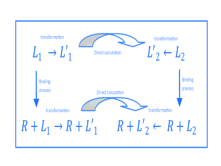
Figure 2: Scheme of the free energy differences in the novel method

In Fig 6 a scheme of the free energies in the novel method is presented. The ligand $L_{\_}1$/ $L_{\_}2$ is transformed into its replica with the long range interactions (VDW and electric) of the different atoms between the systems relaxed $L_{\_}1^{\prime}$/ $L_{\_}2^{\prime}$. The free energy difference between $L_{\_}1^{\prime}$ and $L_{\_}2^{\prime}$ does not need to be calculated since it cancels out ($\Delta F_{\_}{L^{\prime}_{\_}1\rightarrow L^{\prime}_{\_}2}=\Delta F_{\_}{R+L_{\_}1^{\prime}\rightarrow R+L^{\prime}_{\_}2}$). The free energy difference arising from the short range interactions is in many cases the dominant part of the total free energy difference. Hence, for realistic molecular systems, only a capping energy has to be set on the long range potential terms and each system should be transformed into its replica with the long range energy terms of the atoms that are different between the molecules relaxed [24]. This can be applied also for the comparison of molecules with different molecular ring content. Thus, simple comparison between any two systems with the same degrees of freedom can be performed. We write the Hamiltonian in its final form:

$$H^{\prime}_{\_}{A/B}\left(\lambda\right)=\lambda H^{\prime}_{\_}{{}_{\_}{{A_{\_}{dlr}/B_{\_}{dlr}}}}+f(\lambda)H_{\_}{{}{A/B}}$$ (18)

where $H_{\_}{{}_{\_}{{A_{\_}{dlr}/B_{\_}{dlr}}}}$ denote the different long range energy terms. The corresponding calculation of solvation/binding free energies in the case of systems that do not necessitate H-REMD procedure can thus be written:

$$\Delta F_{\_}{A_{\_}{\mathrm{solvation/binding}}\rightarrow B_{\_}{\mathrm{solvation/binding}}}=\int_{\_}0^{1}\left\langle H^{\prime}_{\_}{B_{\_}{dlr}}\right\rangle-\int_{\_}0^{1}\left\langle H^{\prime}_{\_}{A_{\_}{dlr}}\right\rangle$$ (19)

$$+\int_{\_}0^{1}\left\langle H^{\prime}_{\_}{A_{\_}{\mathrm{solvated/bounded}_{\_}{dlr}}}\right\rangle-\int_{\_}0^{1}\left\langle H^{\prime}_{\_}{B_{\_}{\mathrm{solvated/bounded}_{\_}{dlr}}}\right\rangle$$ (20)

We emphasize the fact that in this standard context there is no need to calculate anything besides the calculation mentioned in the equation above. The method has been demonstrated and compared in the context of the direct calculation on systems of a molecule of two atoms in a spherical potential [30].

Discussion

A novel method for calculating free energy difference between systems is presented. This method can be used to calculate the free energy difference between a wide range of systems that have the same degrees of freedom and is highly efficient, robust and simple. In this method there are no large penalties in the running time that originate from the dissimilarity between the systems. Moreover, since the $\lambda$s used in the H-REMD/H-PT procedure are also used as intermediates in the calculation of free energy difference, a convergence for systems with rugged energy landscape is achieved without introducing another sampling dimension. Both in the calculation of the integral for the free energy difference and in the H-REMD/H-PT procedures, the chosen intervals between the $\lambda$s have to be smaller where the internal energy varies significantly, in the free energy difference calculation in order to have good sampling of the function and in H-REMD in order to maintain optimal acceptance rates. Thus, no additional unnecessary $\lambda$s have to be sampled.

In equilibrium methods the hybrid system has one set of coordinates that specifies the configurations of the two systems so the hybrid system often needs to be designed. In addition when the hybrid Hamiltonian involves potentials with more complicated lambda dependence, their derivatives may have to be calculated. The method has the advantage of simplicity since the simulations are performed only on the two (almost) original systems (separate simulations) and the need to relate between the compared systems is eliminated.

Using this method (preceded by virtual screening filtering) an automated free energy calculation that will result in the best candidates may be performed. It is noted that the method can be applied to calculate free energies of systems composed of weakly interacting subsystems (e.g spin system in a magnetic field with weak coupling). There is a provisional patent pending that includes the content of this paper. Prof. D. Harries and Prof. G. Falkovich are acknowledged for the useful comments.

Supplementary Material

Demonstration and comparison

In order to demonstrate the method it was used with all its ingredients in MC simulation to calculate the free energy difference between the systems $A$ and $B$ and this value was compared to the one calculated by numerical integration. Then, in order to asses the efficiency of the method, the free energy difference between the systems was calculated using ThI combined with H-PT (in MC simulation) and the running time of the two methods was compared.

The compared systems are composed of a molecule of two atoms in which one atom is fixed to the origin and the second one is bound to the first by a covalent bond. The second atom in each system is in a $\theta$ dependent potential (in spherical coordinates), containing $\theta^{-12}$ term to represent the VDW repulsive term used in molecular modeling. The potential barrier was chosen to be of typical value of systems with tens of atoms, having rugged energy landscape. The covalent bond length difference was chosen to represent systems with few different atom lengths- see the next section for more details (the values of the pairs of spring constant and covalent bond length were taken from molecular simulation software). The following potential and parameters were used:

$$V_{\_}{A}=\frac{1}{2}k\left(r_{\_}{12}-r_{\_}{eq_{\_}{A}}\right)^{2}-5.5k_{\_}{b}T\cdot\left[sin\left(4\theta\right)-\frac{10^{-8}}{\left(\theta-\frac{3\pi}{8}\right)^{12}}\right]$$ (21)

$$V_{\_}{B}=\frac{1}{2}k\left(r_{\_}{12}-r_{\_}{eq_{\_}{B}}\right)^{2}+5k_{\_}{b}T\cdot\left[sin\left(4\theta\right)+\frac{10^{-8}}{\left(\theta-\frac{5\pi}{8}\right)^{12}}\right]$$ (22)

$$r_{\_}{eq_{\_}{A}}=2.1\,\AA,r_{\_}{eq_{\_}{B}}=1.3\,\AA,k_{\_}{A}=123\,kCal/Mol\AA^{2}$$

$$k_{\_}{B}=428\,kCal/Mol\AA^{2},E_{\_}{cut\,off}=7\,kCal/Mol$$

Here we used the partition function of two atoms with a covalent bond term represented by a harmonic potential that can be written as follows:

$$Z\left(\beta\right)=\frac{1}{l^{3}}\int_{\_}{-\infty}^{\infty}e^{-\beta k\left(r-d\right)^{2}}d^{3}x=\frac{4\pi}{l^{3}}\int_{\_}{0}^{\infty}e^{-\beta k\left(r-d\right)^{2}}r^{2}dr=$$ (23)

$$\frac{\pi\left[\left(2d^{2}\beta k+1\right)\left(erf\left(d\sqrt{\beta k}\right)+1\right)+2\sqrt{\pi}e^{-\beta kd^{2}}d\sqrt{\beta k}\right]}{4l^{3}\left(\beta k\right)^{3/2}}$$ (24)

where $l$ is an arbitrary length. This was used in eq. $\left(17\right)$ to calculate the free energy difference between the systems with the long range interaction relaxed.

The comparison of the method to the numerical integration yielded exactly the same results. The running time of the calculation of the free energy difference performed by the two methods was compared and yielded a factor of $\sim 30$ in favor of the novel method. This factor originates from the extra sampling dimension and the larger number of intermediates needed in ThI combined with H-PT.

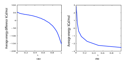
Figure 3: Integrated functions as a function of $\lambda$ (a) Thermodynamic Integration (b) The novel method

In Fig 3 the functions integrated in the two methods are plotted. It can be seen that the difference in magnitude of the integrated function in the novel method is much smaller than this in ThI (factor of $\sim 40$).

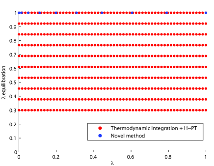
Figure 4: Systems simulated in both methods

In Fig 4 a scheme of the systems simulated in the two methods is presented (each point represents a simulation).

The dissimilarity between the systems that grows with the number of different particles, increases both the number of intermediates (due to a much larger difference in magnitude) and the number of simulation steps (increased variance) as compared with these in the novel method. The difference in the covalent bond description, that reduces the correlation between the systems significantly (the penalties are also not bounded by the capping energy) and has the most dominant effect, has a completely negligible computational cost in the novel method. Thus, the efficiency is increased in 3 multiplicative dimensions.It is here to remind that while the method is highly efficient, its biggest advantage is that it enables many comparisons of molecules with different connectivity. This is since two random molecules are not likely to have the same connectivity.

Correspondence between the toy model and realistic systems in the comparison to Thermodynamic Integration

In the case of realistic compared systems in which the molecules differ in the covalent bond length of one atom (usually when comparing two systems with different connectivity there are many such differences), when the long range energy terms of the atoms that are different between the molecules are relaxed (disregarding the equilibration procedure both in the existing methods and in the novel method for simplicity), the comparison of the methods will yield results that are very similar to the toy model. This is since $\left\langle H_{\_}B-H_{\_}A\right\rangle(\lambda)$ in Thermodynamic Integration will be mainly affected by the changes between the systems. Thus, the functions integrated over in the toy model give good estimation to the ones in the comparison of the realistic systems mentioned above. Since the value of the functions integrated by Thermodynamic Integration is dominated by the covalent bond change (the rest of the difference in the energy terms is negligible as compared with it) it can be written:

$$\left\langle H_{\_}B-H_{\_}A\right\rangle(\lambda)|_{\_}{realistic}\cong\left\langle H_{\_}B-H_{\_}A\right\rangle(\lambda)|_{\_}{toy\,model}\\$$ (25)

Now we turn to show the correspondence in the novel method. We denote the energy terms of the atoms that are different between the realistic compared systems by $H_{\_}{A_{\_}d/B_{\_}d}$. Since these terms are the only ones in the integrated function it can be written:

$$\left\langle H_{\_}{A/B}\right\rangle(\lambda)|_{\_}{realistic}=\left\langle H_{\_}{A_{\_}d/B_{\_}d}\right\rangle(\lambda)|_{\_}{realistic}\thicksim\left\langle H_{\_}{A/B}\right\rangle(\lambda)|_{\_}{toy\,model}\\$$ (26)

In this case there will be similar values since the energy values of the non covalent energy terms are bounded by $E_{\_}{cap}$ and thus the average value is of typical value of $E_{\_}{capping}$. Here the covalent bond energy term is notf included in $H_{\_}{A_{\_}d/B_{\_}d}$. The parameters in the toy model for the covalent bond lengths and strengths are realistic and were taken from simulation software.

Appendix

Explanation of the capping

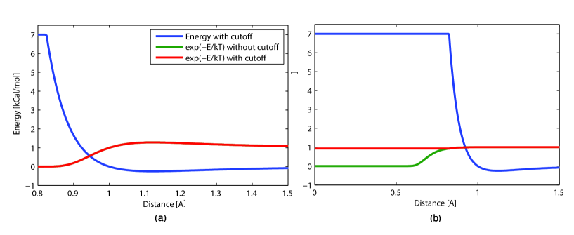
Figure 5: Energy and $\exp(-E/kT)$ as a function of distance for the potential $r^{12}-r^{-6}$ with $E_{\_}{cap}$=7kCal/mol (a) at $\lambda=1$ (b) at $\lambda=0.01$

In Fig 5 energy and $\exp(-E/kT)$ as a function of distance for the potential $r^{12}-r^{-6}$ are plotted at $\lambda=1$ and at $\lambda=0.01$. It can be seen that the cap energy has a negligible effect on the probability distribution at $\lambda=1$ and that at small $\lambda$s the capping of the energy enables the equation of the partition functions. It is noted that the capping has a negligible effect on realistic molecular systems independently of the atoms whose long range potential is being relaxed. This is since each atom has an average potential energy of typical value of $k_{\_}{B}T$ and since the denisty of states for $E>E_{\_}{\mathrm{cutoff}}$ is very low (dual effect). In addition we mention that the force in this range is zero which is legitimate for MD simulations since each atom has a thermal velocity and is also affected by other potentials (this case also exist for VdW and coulomb potentials at large distances). It is noted that a switching function between the standard long range potential and the flat potential is needed in order to ensure continuity in the derivative that will enable the integration over the equations of motion in MD to be valid. In addition, the capping of the enegy removes the limitation in the existing methods in which the electric potential terms have to be removed before the Lennard Jones terms in order to avoid divergence.

The remaining free energy difference

We now turn to show how to treat the calculation of the remaining free energy difference. This will be done in the context of direct free energy calculation between the systems and in the context of the Thermodynamic Cycle.

The context of direct calculation can be used to calculate the free energy difference between two different molecules. This direct calculation is applicable to chemical reactions in which the molecules are different and to the best of our knowledge has not been suggested. The context of the Thermodynamic Cycle is for calculating the free energy difference between the same system (keeping its covalent structure) in two states. This has many applications which include solvation and binding free energies and is here presented in a systematic derivation that enables to keep constant (almost) all the short range energy terms and even some long range potentials, enabling high phase space overlap between the compared systems. While this was derived independently, it has similarities with the derivation in [36] which froms the basis of the relevant state of the art techniques. As compared to the existing practices, here more terms can remain constant in the transformation (e.g long range potentials between the different atoms).

Direct calculation

The calculation of the free energy factors is based on the following change of variables:

$$d\Omega=\prod_{\_}{i=1}^{n}d\mathbf{r^{\prime}_{\_}{i}}=d\mathbf{r^{\prime}_{\_}{1}}\prod_{\_}{i=2}^{k}d\mathbf{r{}_{\_}{i}}\prod_{\_}{i=k+1}^{n}d\mathbf{r{}_{\_}{i}}=\prod_{\_}{i=1}^{k}d\mathbf{r^{\prime}_{\_}{i}}\prod_{\_}{i=k+1}^{n}r_{\_}{i}^{2}sin\theta_{\_}{i}drd\theta d\phi$$

where $\mathbf{r_{\_}{i}}=\mathbf{r^{\prime}_{\_}{i}}-\mathbf{r^{\prime}_{\_}{f\left(i\right)}}$,$r^{\prime}_{\_}{f\left(i\right)}$ is the location of another atom that is bounded to atom $i$ (left for choice), $1..k$ denote the similar atoms and $k+1,...,n$ denote the different atoms between the compared molecules.

Next it will be assumed that the part in the molecule that is different includes only short range interactions and in the beginning of each sub-system there is one dihedral terms and the improper dihedral term is relaxed. The molecule is first divided into elements of standard covalent bonds, bond junctions and of more complex structures that include molecular rings. Since each of the short range potentials depend on one independent variable the the integration in each element is independent of the others. Thus the integrals can be performed separately and then multiplied to yield the partition function. We write these free energy factors explicitly:

Covalent bond

The partition function of a covalent bond in Spherical Coordinates can be written as follows:

$$Z_{\_}c=\int e^{-\frac{\beta k_{\_}c\left(r-d\right)^{2}}{2}}r^{2}dr=\frac{\pi^{2}\left[\left(2d^{2}\beta k_{\_}c+1\right)\left(erf\left(d\sqrt{\beta k_{\_}c}\right)+1\right)+2\sqrt{\pi}e^{-\beta k_{\_}cd^{2}}d\sqrt{\beta k_{\_}c}\right]}{l^{3}\left(\beta k_{\_}c\right)^{3/2}}$$ (27)

where $l$ is an arbitrary length ($l^{3}$ cancels out in comparisons).

Two Bonds Junctions

When considering the case of a Linear/Bent molecular shapes, it can be seen that in most cases when varying the bond angle, the rest of the molecule moves as a rigid body. Since the spherical coordinates representation includes three independent variables, varying a bonding angle is decoupled from all the other degrees of freedom of the molecule. Hence the calculation of free energy factors, which arise from bonding potential terms that are different between the compared molecules, is straightforward. One of the most common bonding angles potentials is the following:

$$V_{\_}{b}\left(\theta\right)=\frac{1}{2}k_{\_}{\theta}\left(\theta-\theta_{\_}{0}\right)^{2}$$ (28)

So the integration over the corresponding degree of freedom can be written as:

$$Z_{\_}{b}=\int e^{-\beta V_{\_}{b}}d\Omega=\int e^{-\frac{\beta k_{\_}{\theta}}{2}\left(\theta-\theta_{\_}{0}\right)^{2}}sin\theta d\theta=$$ (29)

$$\frac{1}{2\sqrt{\beta k_{\_}{\theta}}}e^{-i\theta_{\_}{0}-\frac{1}{2\beta k_{\_}{\theta}}}\sqrt{\frac{\pi}{2}}\left(i\text{Erf}\left[\frac{i-\theta_{\_}{0}\beta k_{\_}{\theta}+\beta k_{\_}{\theta}\pi}{\sqrt{2\beta k_{\_}{\theta}}}\right]+\text{Erfi}\left[\frac{1+i\theta_{\_}{0}\beta k_{\_}{\theta}}{\sqrt{2\beta k_{\_}{\theta}}}\right]-ie^{2i\theta_{\_}{0}}\left(\text{Erf}\left[\frac{i+\theta_{\_}{0}k_{\_}{\theta}}{\sqrt{2\beta k_{\_}{\theta}}}\right]-i\text{Erfi}\left[\frac{1+i\beta k_{\_}{\theta}(\pi-\theta_{\_}{0})}{\sqrt{2\beta k_{\_}{\theta}}}\right]\right)\right)$$ (30)

This expression is real for positive and real values of $k_{\_}{\theta},\beta$ and $\theta_{\_}{0}$.

When varying a dihedral angle, the potential term value depends on the orientation of first bond (which determines the axis from which the dihedral angle is measured). However, since the integration has to be performed over all the range $\left[0,2\pi\right]$, varying the $\phi$ angle will yield a factor which is independent of the location of the first bond. Thus, the integration does not depend on the direction of the first bond and is straightforward. The commonly used dihedral angles potential is of the following type:

$$V_{\_}{d}\left(\phi_{\_}{ijkl}\right)=k_{\_}{\phi}\left(1+cos\left(n\phi-\phi_{\_}{s}\right)\right)$$ (31)

The integration over this degree of freedom yields the following result:

$$Z_{\_}{d}=\int e^{-\beta V_{\_}{d}}d\Omega=\int e^{-\beta k_{\_}{\phi}\left(1+cos\left(n\phi-\phi_{\_}{s}\right)\right)}d\phi=2\pi e^{-\beta k_{\_}{\phi}}I_{\_}{0}\left(\beta k_{\_}{\phi}\right)$$ (32)

where $I_{\_}{0}\left(\beta k_{\_}{\phi}\right)$ is Bessel function of the first kind at $\beta k_{\_}{\phi}$ which is defined as follows:

$$I_{\_}{0}\left(x\right)=\sum_{\_}{l=0}^{\infty}\frac{\left(-1\right)^{l}}{2^{2l}\left(l!\right)^{2}}x^{2l}$$ (33)

Three or more Bonds Junctions

Molecule shapes can include monomer that splits into more than one monomer. Such examples are the trigonal planar, tetrahedral trigonal pyramidal etc. In these cases there is coupling between the monomers which will necessitate numerical integration. This can be performed using the Spherical law of cosines which can be written as follows:

$$cos\left(\theta_{\_}{12}\right)=cos\left(\theta_{\_}{1}\right)cos\left(\theta_{\_}{2}\right)+sin\left(\theta_{\_}{1}\right)sin\left(\theta_{\_}{2}\right)cos\left(\Delta\phi\right)$$ (34)

where $\theta_{\_}{1},\theta_{\_}{2}$ denote the bond angles of two bonds with respect to the principal bond and $\theta_{\_}{12},\Delta\phi$ denote the bond angle and the difference in $\phi$ angle between these two bonds respectively. Usually in these cases there is one dihedral angle energy term which is between one of the bonds, the principal bond and a previous bond. Since the integration over the other degrees of freedom yields a factor that is independent of the value of $\phi$, the integrations can be treated as decoupled. Thus, the integration for the case of one monomer that splits into two can be written as follows:

$$Z=\int e^{-\beta\left(V_{\_}{b}+V_{\_}{d}\right)}d\Omega=Z_{\_}{d}Z_{\_}{b}$$ (35)

where

$$Z_{\_}{d}=2\pi e^{-\beta k_{\_}{\phi}}I_{\_}{0}\left(\beta k_{\_}{\phi}\right)$$

and

$$Z_{\_}{b}=\int e^{-\frac{\beta}{2}\left[k_{\_}{1}^{\theta}\left(\theta_{\_}{1}-\theta_{\_}{1}^{0}\right)^{2}+k_{\_}{2}^{\theta}\left(\theta_{\_}{2}-\theta_{\_}{2}^{0}\right)^{2}+k_{\_}{12}^{\theta}\left(\theta_{\_}{12}-\theta_{\_}{12}^{0}\right)^{2}\right]}sin(\theta_{\_}{1})sin(\theta_{\_}{2})d\theta_{\_}{1}d\theta_{\_}{2}d\phi_{\_}{2}$$ (36)

For the general case it can be written as follows:

$$Z_{\_}{b}=\int\prod_{\_}{i}e^{-\frac{\beta}{2}k_{\_}{i}^{\theta}\left(\theta_{\_}{i}-\theta_{\_}{i}^{0}\right)^{2}}\prod_{\_}{i>j}e^{-\frac{\beta}{2}k_{\_}{ij}^{\theta}\left(\theta_{\_}{ij}-\theta_{\_}{ij}^{0}\right)^{2}}\prod_{\_}{i}sin\theta_{\_}{i}d\theta_{\_}{i}\prod_{\_}{i\geq 2}d\phi_{\_}{i}$$ (37)

where $\theta_{\_}{ij}$ can be calculated from (34). In case there are any energy terms that introduce complexity they can be relaxed in the transformation.

These free energy factors can be substituted in:

$$\Delta F_{\_}{B_{\_}{dsr}\rightarrow A_{\_}{dsr}}=k_{\_}{B}T\left[\sum_{\_}{i}lnZ_{\_}{B_{\_}{c_{\_}{i}}}+\sum_{\_}{i}lnZ_{\_}{B_{\_}{b_{\_}{i}}}+\sum_{\_}{i}lnZ_{\_}{B_{\_}{d_{\_}{i}}}-\left(\sum_{\_}{i}lnZ_{\_}{A_{\_}{c_{\_}{i}}}+\sum_{\_}{i}lnZ_{\_}{A_{\_}{b_{\_}{i}}}+\sum_{\_}{i}lnZ_{\_}{A_{\_}{d_{\_}{i}}}\right)\right]$$ (38)

to give the remaining free energy difference.

Thus, we can write in terms of the partition functions:

$$Z\rightarrow Z_{\_}{\mathrm{common\,int}}\prod_{\_}{i=1}^{l}Z_{\_}{c_{\_}{i}}\prod_{\_}{i=1}^{m}Z_{\_}{d_{\_}{i}}\prod_{\_}{i=1}^{p}Z_{\_}{2b_{\_}{i}}\prod_{\_}{i=1}^{q}Z_{\_}{3b_{\_}{i}}\prod_{\_}{i=1}^{r}Z_{\_}{\mathrm{complex}_{\_}{i}}$$

where $Z_{\_}{\mathrm{common\,int}}$ represents the partition function of the common part between the compared molecules that is interacting with the environment and $Z_{\_}{c_{\_}{i}}$ and $Z_{\_}{d_{\_}{i}}$ represent the $i$th covalent bond and dihedral angle partition function respectively. $Z_{\_}{2b_{\_}{i}}$ and $Z_{\_}{3b_{\_}{i}}$ represent the $i$th two bond and three or more bond junctions respectively and $Z_{\_}{\mathrm{complex}_{\_}{i}}$ represents the $i$th complex structure partition function. The arrow represents the transformation $\lambda=1\rightarrow 0$.

The context of the Thermodynamic Cycle

For the standard case in which the Thermodynamic Cycle is used the change of variables takes the form:

$$d\Omega=\prod_{\_}{i}^{n}d\mathbf{r^{\prime}_{\_}{i}}=d\mathbf{r^{\prime}_{\_}{1}}\prod_{\_}{i=2}^{k}d\mathbf{r{}_{\_}{i}}d\mathbf{r{}_{\_}{k+1}}\prod_{\_}{i=k+2}^{n}d\mathbf{r{}_{\_}{i}^{{}^{\prime}}}=$$

$$d\mathbf{r^{\prime}_{\_}{1}}\prod_{\_}{i=2}^{k}d\mathbf{r{}_{\_}{i}}r_{\_}{k+1}^{2}sin\theta_{\_}{k+1}dr_{\_}{k+1}d\theta_{\_}{k+1}d\phi_{\_}{k+1}\prod_{\_}{i=k+2}^{n}d\mathbf{r{}_{\_}{i}}$$

This change of variables is motivated by the fact that the part that is different between the molecules includes only short range interactions and in the beginning of the different part there is one dihedral angle and the improper dihedral term is relaxed.

Thus, we can write in terms of the partition functions:

$$Z\left(\mathbf{r^{\prime}_{\_}{1}},\mathbf{r{}_{\_}{2}},..,\mathbf{r_{\_}{n}}\right)\rightarrow Z_{\_}{\mathrm{common\,int}}\left(\mathbf{r^{\prime}_{\_}{1}},\mathbf{r{}_{\_}{2}},..,\mathbf{r_{\_}{k}}\right)Z_{\_}{\mathrm{diff\,non\,int}}\left(\mathbf{r_{\_}{k+1,...,}r_{\_}{n}}\right)$$

where $Z_{\_}{\mathrm{diff\,non\,int}}$ denotes the partition function of the different part of the molecule that does not interact with the environment and the arrow symbolizes the transformation in which the long range energy terms are relaxed.

In the case of totally different molecules it can thus be written:

$$Z\rightarrow Z_{\_}{\mathrm{diff\,non\,int}}$$

Here we made use of the fact that if the potential in the separation point between the common and different parts of the molecule depends on the spherical variables then there is decoupling between the common and different parts of the molecule. It is noted that $Z_{\_}{\mathrm{diff\,non\,int}}$ cancels out in the Thermodynamic cycle.

In case there are improper dihedral term or more than one dihedral term at the separation point (non common), we can simply relax them in the transformation. Thus $Z_{\_}{\mathrm{diff\,non\,int}}$ does not need to be calculated and it can include any short range potentials including dihedral and improper dihedrals. This treatment for the usual case in which the Thermodynamic Cycle is used demonstrates that the method is general and can be automated. For clarity we summarize: free energy calculations in equilibrium methods are usually performed in the context of the Thermodynamic cycle. Since the partition function can simply be splitted to the common and different parts and the free energy associated with $Z_{\_}{\mathrm{diff\,non\,int}}$ cancels out in the Thermodynamic cycle, there is no need to calculate the free energy difference. It is noted that the long range terms between terms the different atoms can remain constant. In addition it might be that if the the long range terms between the different atoms and the common environement (e.g water in binding) are kept constant it may have a small effect on the free energy.

The Thermodynamic cycle of the novel method

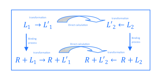
Figure 6: Scheme of the free energy differences in the novel method

In Fig 6 a scheme of the free energies in the novel method is presented. The ligand $L_{\_}1$/ $L_{\_}2$ is transformed into its replica with the long range interactions (VDW and electric) of the different atoms between the systems relaxed $L_{\_}1^{\prime}$/ $L_{\_}2^{\prime}$. The free energy difference between $L_{\_}1^{\prime}$ and $L_{\_}2^{\prime}$ can be directly calculated but does not need to be since it cancels out ($\Delta F_{\_}{L^{\prime}_{\_}1\rightarrow L^{\prime}_{\_}2}=\Delta F_{\_}{R+L_{\_}1^{\prime}\rightarrow R+L^{\prime}_{\_}2}$). The free energy difference arising from the direct calculation is in many cases the dominant part of the total free energy difference. It can be written as follows:

$$\Delta F_{\_}{L_{\_}1\rightarrow R+L_{\_}1}-\Delta F_{\_}{L_{\_}2\rightarrow R+L_{\_}2}=\Delta F_{\_}{L_{\_}1\rightarrow L^{\prime}_{\_}1}+\Delta F_{\_}{L^{\prime}_{\_}1\rightarrow L^{\prime}_{\_}2}-\Delta F_{\_}{L_{\_}2\rightarrow L^{\prime}_{\_}2}-\left(\Delta F_{\_}{R+L_{\_}1\rightarrow R+L^{\prime}_{\_}1}+F_{\_}{R+L_{\_}1^{\prime}\rightarrow R+L^{\prime}_{\_}2}-\Delta F_{\_}{R+L_{\_}2\rightarrow R+L^{\prime}_{\_}2}\right)$$

$$=\Delta F_{\_}{L_{\_}1\rightarrow L^{\prime}_{\_}1}-\Delta F_{\_}{L_{\_}2\rightarrow L^{\prime}_{\_}2}-\left(\Delta F_{\_}{R+L_{\_}1\rightarrow R+L^{\prime}_{\_}1}-\Delta F_{\_}{R+L_{\_}2\rightarrow R+L^{\prime}_{\_}2}\right)$$ (39)

Thus, the relative binding free energy can be calculated. This scheme is also relevant for relative free energy of solvation in which $R$ will represent the solvent instead of the receptor.

Use of the method for comparing two molecular systems

As an example the simple molecules Benzoic acid and Toluene, that can be compared with this method, are presented.

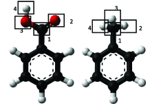
Figure 7: Benzoic acid (left) and Toluene (right) molecules

Calculating the free energy difference can be easily done in the method by relaxing only the long range (VDW and electric) energy terms of the atoms that are different between the molecules (atoms 2-4) in the transformation A/B to A’/B’ by multiplying (only) them by $\lambda=1\rightarrow 0$, decoupling their long range interactions from the rest of the molecule (and all their interactions with the environment). Now the partition function of each system can be separated into the complex PF of ring+atom $1$ which is identical between the systems (cancels out) and other simple decoupled PFs (direct calculation) or PF of the different part (TC) . The remaining difference in the free energy can be easily calculated by integration in the direct calculation and in the thermodynamic cycle it does not have to be calculated (cancels out). This can be applied also for the comparison of molecules with different molecular ring content (e.g Cyclobutane and Benzene or larger molecules differing by such entities). Thus, simple comparison between any two systems with the same degrees of freedom can be performed.

References

- [1] Christophe Chipot and Andrew Pohorille. Free energy calculations: theory and applications in chemistry and biology, volume 86. Springer, 2007.
- [2] Daniel M Zuckerman. Equilibrium sampling in biomolecular simulations. Annual review of biophysics, 40:41–62, 2011.
- [3] D. Frenkel and B. Smit. Understanding molecular simulation: from algorithms to applications. Academic Press, Inc. Orlando, FL, USA, 1996.
- [4] M.R. Shirts, D.L. Mobley, and J.D. Chodera. Alchemical free energy calculations: Ready for prime time? Annual Reports in Computational Chemistry, 3:41–59, 2007.
- [5] Kurt Binder and Dieter W Heermann. Monte Carlo simulation in statistical physics: an introduction. Springer, 2010.
- [6] Peter Kollman. Free energy calculations: applications to chemical and biochemical phenomena. Chemical Reviews, 93(7):2395–2417, 1993.
- [7] Y. Deng and B. Roux. Computations of standard binding free energies with molecular dynamics simulations. The Journal of Physical Chemistry B, 113(8):2234–2246, 2009.
- [8] C.J. Woods, M. Malaisree, S. Hannongbua, and A.J. Mulholland. A water-swap reaction coordinate for the calculation of absolute protein-ligand binding free energies. Journal of Chemical Physics, 134(5):4114, 2011.
- [9] TP Straatsma and HJC Berendsen. Free energy of ionic hydration: Analysis of a thermodynamic integration technique to evaluate free energy differences by molecular dynamics simulations. The Journal of chemical physics, 89:5876, 1988.
- [10] Ilja V Khavrutskii and Anders Wallqvist. Computing relative free energies of solvation using single reference thermodynamic integration augmented with hamiltonian replica exchange. Journal of chemical theory and computation, 6(11):3427–3441, 2010.
- [11] William L Jorgensen, James M Briggs, and Jiali Gao. A priori calculations of pka’s for organic compounds in water. the pka of ethane. Journal of the American Chemical Society, 109(22):6857–6858, 1987.
- [12] X.Y. Meng, H.X. Zhang, M. Mezei, and M. Cui. Molecular docking: A powerful approach for structure-based drug discovery. Current Computer-Aided Drug Design, 7(2):146–157, 2011.
- [13] William L Jorgensen. Efficient drug lead discovery and optimization. Accounts of chemical research, 42(6):724–733, 2009.
- [14] John D Chodera, David L Mobley, Michael R Shirts, Richard W Dixon, Kim Branson, and Vijay S Pande. Alchemical free energy methods for drug discovery: progress and challenges. Current opinion in structural biology, 21(2):150–160, 2011.
- [15] C.H. Bennett. Efficient estimation of free energy differences from monte carlo data. Journal of Computational Physics, 22(2):245–268, 1976.
- [16] S. Kumar, J.M. Rosenberg, D. Bouzida, R.H. Swendsen, and P.A. Kollman. The weighted histogram analysis method for free-energy calculations on biomolecules. i. the method. Journal of Computational Chemistry, 13(8):1011–1021, 1992.
- [17] R.W. Zwanzig. High-temperature equation of state by a perturbation method. i. nonpolar gases. The Journal of Chemical Physics, 22:1420, 1954.
- [18] J.G. Kirkwood. Statistical mechanics of fluid mixtures. The Journal of Chemical Physics, 3:300, 1935.
- [19] TP Straatsma and JA McCammon. Multiconfiguration thermodynamic integration. The Journal of chemical physics, 95:1175, 1991.
- [20] C. Jarzynski. Nonequilibrium equality for free energy differences. Physical Review Letters, 78(14):2690, 1997.
- [21] DA Hendrix and C. Jarzynski. A fast growth method of computing free energy differences. The Journal of Chemical Physics, 114:5974, 2001.
- [22] G.E. Crooks. Path ensembles averages in systems driven far-from-equilibrium. Arxiv preprint cond-mat/9908420, 1999.
- [23] E. Darve and A. Pohorille. Calculating free energies using average force. The Journal of Chemical Physics, 115:9169, 2001.
- [24] To be published.
- [25] Michael R Shirts. Best practices in free energy calculations for drug design. In Computational Drug Discovery and Design, pages 425–467. Springer, 2012.
- [26] A. Farhi, G. Hed, M. Bon, N. Caticha, C.H. Mak, and E. Domany. Temperature integration: an efficient procedure for calculation of free energy differences. Arxiv preprint cond-mat/1212.3978, 2012.
- [27] James C Phillips, Rosemary Braun, Wei Wang, James Gumbart, Emad Tajkhorshid, Elizabeth Villa, Christophe Chipot, Robert D Skeel, Laxmikant Kale, and Klaus Schulten. Scalable molecular dynamics with namd. Journal of computational chemistry, 26(16):1781–1802, 2005.
- [28] Berk Hess, Carsten Kutzner, David Van Der Spoel, and Erik Lindahl. Gromacs 4: Algorithms for highly efficient, load-balanced, and scalable molecular simulation. Journal of chemical theory and computation, 4(3):435–447, 2008.
- [29] A. Farhi. Msc thesis. Arxiv preprint cond-mat/1212.4081, 2011.
- [30] Supplementary material.
- [31] Floris P Buelens and Helmut Grubmüller. Linear-scaling soft-core scheme for alchemical free energy calculations. Journal of Computational Chemistry, 33(1):25–33, 2012.
- [32] A.M. Ferrenberg and R.H. Swendsen. New monte carlo technique for studying phase transitions. Physical review letters, 61(23):2635, 1988.
- [33] U.H.E. Hansmann. Parallel tempering algorithm for conformational studies of biological molecules. Chemical Physics Letters, 281(1-3):140–150, 1997.
- [34] D.J. Earl and M.W. Deem. Parallel tempering: Theory, applications, and new perspectives. Physical Chemistry Chemical Physics, 7(23):3910–3916, 2005.
- [35] H. Fukunishi, O. Watanabe, and S. Takada. On the hamiltonian replica exchange method for efficient sampling of biomolecular systems: Application to protein structure prediction. The Journal of chemical physics, 116:9058, 2002.
- [36] Stefan Boresch, Franz Tettinger, Martin Leitgeb, and Martin Karplus. Absolute binding free energies: a quantitative approach for their calculation. The Journal of Physical Chemistry B, 107(35):9535–9551, 2003.