Quantum critical Kondo destruction in the Bose-Fermi Kondo model with a local transverse field

Abstract

Recent studies of the global phase diagram of quantum-critical heavy-fermion metals prompt consideration of the interplay between the Kondo interactions and quantum fluctuations of the local moments alone. Toward this goal, we study a Bose-Fermi Kondo model (BFKM) with Ising anisotropy in the presence of a local transverse field that generates quantum fluctuations in the local-moment sector. We apply the numerical renormalization-group method to the case of a sub-Ohmic bosonic bath exponent and a constant conduction-electron density of states. Starting in the Kondo phase at zero transverse-field, there is a smooth crossover with increasing transverse field from a fully screened to a fully polarized impurity spin. By contrast, if the system starts in its localized phase, then increasing the transverse field causes a continuous, Kondo-destruction transition into the partially polarized Kondo phase. The critical exponents at this quantum phase transition exhibit hyperscaling and take essentially the same values as those of the BFKM in zero transverse field. The many-body spectrum at criticality varies continuously with the bare transverse field, indicating a line of critical points. We discuss implications of these results for the global phase diagram of the Kondo lattice model.

I Introduction

Heavy fermions form a class of rare-earth based intermetallic compounds that has attracted sustained attention.si_science10 Recent years have seen intensive effort, both in theory and experiment, to understand the unusual properties exhibited by these materials over a temperature range above a quantum critical point (QCP).stewart ; gegenwart_natphys08 ; HvL The most typical cases involve a zero-temperature transition from an antiferromagnetically ordered state to a paramagnetic heavy Fermi-liquid. A particularly notable feature of the quantum-critical regime is the non-Fermi liquid behavior, which has been observed in transport, thermodynamic, and other properties in a number of compounds. Two fundamentally different classes of quantum critical points have been proposed theoretically. The spin-density-wave QCPshertz represent the quantum-mechanical extension of the classical Landau-Ginzburg-Wilson framework, describing criticality solely in terms of fluctuations of a magnetic order parameter. By contrast, the locally critical picturelcqpt:01 ; lcqpt:03 ; colemanetal is “beyond-Landau” in that it invokes the destruction of the heavy quasiparticles at the transition. Such a Kondo destruction introduces new critical degrees of freedom beyond order-parameter fluctuations. A microscopic theory of local quantum criticalitylcqpt:01 ; lcqpt:03 has been formulated in terms of extended dynamical mean-field theory (EDMFT),SmithSi ; Chitra:00 in which the Kondo lattice model is mapped to an effective quantum impurity problem: the Bose-Fermi Kondo model (BFKM) with self-consistently determined densities of states for the fermionic conduction band and for the bosonic bath.

Experimental evidence for local quantum criticality has come from systematic studies in several heavy-fermion materials. In YbRh₂Si₂ and CeRhIn₅, the large Fermi surface of the paramagnetic metal phase has been shown to collapse at the antiferromagnetic QCP,paschen04 ; friedemann10 ; shishido providing direct evidence for a critical destruction of the Kondo effect. The critical dynamical spin susceptibility at the QCP in Au-doped CeCu₆ departs drastically from the predictions of the spin-density-wave picture, instead satisfying $\omega/T$ scaling and displaying a fractional exponent in the frequency and temperature dependence over a large region of the Brillouin zone.schroder Such scaling properties have been captured in EDMFT calculations for Kondo lattice models.lcqpt:01 ; lcqpt:03 ; Grempel.03 ; ZhuGrempelSi ; Glossop.07 ; Zhu.07

More recently, the notion of Kondo destruction has been incorporated into a global zero-temperature phase diagram for heavy fermions.Si:10+06 The phase diagram, proposed for the Kondo lattice model, is shown in Fig. 1, where the abscissa represents the Kondo exchange coupling between local moments and conduction electrons, while the ordinate G parameterizes quantum fluctuations of the local moments. Three different sequences of quantum phase transitions can connect a Kondo-destroyed antiferromagnet to the Kondo-entangled paramagnetic heavy-fermion state. This diagram provides a framework for understanding not only the examples of local quantum-critical behavior described above, but also the detachment of the Kondo destruction transition from the antiferromagnetic transition as evidenced11 ; 12 ; 13 in Ge- and Ir-doped YbRh₂Si₂ and in YbAgGe. The global phase diagram has recently been employed to understand the dimensional tuning of the quantum-critical behavior in heavy-fermion systems,custers12 and has served as a motivation for a recent flurry of experiments on heavy-fermion materials with geometrically frustrated lattices.kim_aronson13 ; mun13 ; fritsch13 ; Khalyavin13

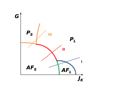
Figure 1: (Color online) Schematic $T=0$ phase diagram proposed for heavy-fermion metals described by a Kondo lattice.Si:10+06 $J_{K}$ is the antiferromagnetic Kondo coupling between local moments and conduction electrons, while $G$ parameterizes increasing magnetic frustration or spatial dimensionality. Solid lines indicate phase boundaries. Dashed lines labeled I, II, and III represent three different types of route between the paramagnetic heavy Fermi-liquid phase having a large Fermi surface (P${}_{\textrm{L}}$) and an antiferromagnetic Kondo-destroyed phase with a small Fermi surface (AF${}_{\textrm{S}}$)

.

The key feature of the global phase diagram for heavy fermions is the interplay between quantum fluctuations related to the Kondo effect and those associated with the local moments alone. Consider the Kondo lattice Hamiltonian $H_{\mathrm{KL}}=H_{c}+H_{I}+H_{K}$, where $H_{c}$ and $H_{I}$ represent a conduction-electron band and a lattice of exchange-coupled local moments, respectively, and $H_{K}$ specifies the Kondo coupling between these two sectors. In situations where the local moments exhibit Ising (easy-axis) anisotropy, quantum fluctuations of these moments can readily be generated through application of a transverse magnetic field. For example, in the stand-alone transverse-field Ising model described by $H=H_{I}=\sum_{ij}I_{ij}S_{i}^{z}S_{j}^{z}+\Delta\sum_{i}S_{i}^{x}$, the transverse field $\Delta$ introduces quantum fluctuations and sufficiently large values of $\Delta$ suppress any magnetic order. In other words, $\Delta$ provides a realization of the parameter $G$ in Fig. 1. Within the EDMFT treatment of $H_{\mathrm{KL}}$, this interplay of fluctuations can be described using a self-consistent BFKM with a static transverse magnetic field. As a nontrivial first step towards solving this problem, we are led to consider the impurity version of this problem without the imposition of self-consistency.

This paper reports numerical renormalization-group (NRG) results for the BFKM in the presence of a local transverse magnetic field $\Delta$. The conduction-electron density of states is taken to be structureless, while the bosonic bath is assumed to be characterized by a spectral exponent $s$ that takes a sub-Ohmic value $0<s<1$. For $\Delta=0$, this model exhibits a Kondo-destruction QCP separating a Kondo or strong-coupling phase, in which the impurity spin is completely quenched at temperature $T=0$, from a localized phase in which spin-flip exchange scattering is suppressed and the impurity exhibits a local moment with a Curie magnetic susceptibility.Zhu:02 ; Zarand:02 ; Glossop:05+07 For any combination of Kondo and bosonic couplings that, at $\Delta=0$, places the system within the Kondo phase, increasing the transverse field produces a smooth crossover to a fully polarized impurity spin without the appearance of a quantum phase transistion. For couplings that localize the impurity spin in the absence of a transverse field, increasing such a field eventually causes a continuous, Kondo-destruction transition into the partially polarized Kondo phase. The critical exponents at this quantum phase transition are found, for the particular case of bosonic bath exponent $s=0.8$, to exhibit hyperscaling and to take essentially the same values as those of the BFKM in zero transverse field. The critical NRG spectrum varies continuously with the bare transverse field, indicating a line of critical points.

The remainder of the paper is organized as follows. Section II defines the model and briefly describes the NRG solution method. Section III demonstrates the existence of a Kondo-destruction transition in the BFKM at particle-hole symmetry in the presence of a bosonic bath characterized by a sub-Ohmic spectral exponent $s=0.8$. In Sec. IV we interpret the critical spectra reached for different values of the transverse field as evidence for a line of renormalization-group (RG) fixed points. The accuracy of our calculated critical exponents is addressed in an Appendix.

II Model, Qualitative Expectations and Solution Method

II.1 Bose-Fermi Kondo model with a transverse field

The Hamiltonian for the Ising-anisotropic BFKM with a transverse field can be written

$$H_{\mathrm{BFKM}}=\sum_{\mathbf{k},\sigma}\epsilon_{\mathbf{k}}c_{\mathbf{k}\sigma}^{{\dagger}}c_{\mathbf{k}\sigma}^{\phantom{{\dagger}}}+\frac{J_{K}}{2}\,\mathbf{S}\cdot\!\!\!\sum_{\mathbf{k},\mathbf{k}^{\prime},\sigma,\sigma^{\prime}}\!\!\!c_{\mathbf{k}\sigma}^{{\dagger}}\bm{\sigma}_{\sigma\sigma^{\prime}}c_{\mathbf{k}^{\prime}\sigma^{\prime}}^{\phantom{{\dagger}}}\\ +\sum_{q}\omega_{q}\phi_{q}^{{\dagger}}\phi_{q}^{\phantom{{\dagger}}}+S_{z}\sum_{q}g_{q}\bigl{(}\phi_{q}^{\phantom{{\dagger}}}+\phi_{-q}^{{\dagger}}\bigr{)}+\Delta S_{x},$$ (1)

where $\epsilon_{\mathbf{k}}$ is the dispersion for a band of noninteracting conduction electrons, $J_{K}>0$ is the antiferromagnetic Kondo coupling between a spin-$\frac{1}{2}$ local moment $\mathbf{S}$ and the spin density of conduction electrons at the impurity site, $g_{q}$ is the coupling of the impurity spin $z$ component to a bosonic degree of freedom with annihilation operator $\phi_{q}$, and $\Delta\geq 0$ is the transverse field. We work in units where $g\mu_{B}=k_{B}=\hbar=1$.

Throughout the paper, we assume a featureless metallic conduction electron band described by the density of states

$$\rho(\epsilon)=\sum_{\mathbf{k}}\delta(\epsilon-\epsilon_{\mathbf{k}})=\rho_{0}\,\Theta(D-|\epsilon|),$$ (2)

where $D$ is the half-bandwidth and $\Theta$ is the Heaviside step function, allowing definition of a dimensionless exchange coupling $\rho_{0}J_{K}$ between the band and the impurity spin. We denote by $T_{K}^{0}$ the Kondo temperature associated with this exchange in the absence of any bosonic coupling. The bosonic spectral function is taken to be

$$B\left(\omega\right)\equiv\pi\sum_{q}g_{q}^{2}\delta\bigl{(}\omega-\omega_{q}\bigr{)}=B_{0}\,\omega_{0}^{1-s}\omega^{s}\,\Theta(\omega)\,\Theta(\omega_{0}-\omega),$$ (3)

where $\omega_{0}$ is a high-energy cutoff and $B_{0}$ is a dimensionless effective coupling between the impurity spin and the bosonic bath. Previous studiesZhu:02 ; Glossop:05+07 ; 27 have taken $g_{q}=g$, in which case $B_{0}={(K_{0}g)}^{2}$ with $K_{0}$ being determined by the bath density of states. Henceforth, we refer to $B_{0}$ as the effective coupling to the dissipative bath. Values of the exponent $s<1$, $s=1$ and $s>1$ correspond to sub-Ohmic, Ohmic and super-Ohmic baths, respectively.

II.2 Qualitative Considerations

The BFKM with $\Delta=0$ and a sub-Ohmic bath exponent $0<s<1$ features an unstable fixed point lying on a separatrix in the $B_{0}$-$J_{\perp}$ plane [see Fig. 2(a)].

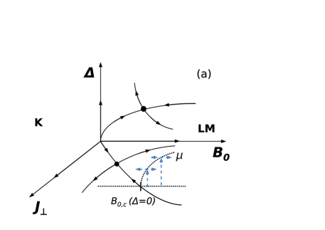
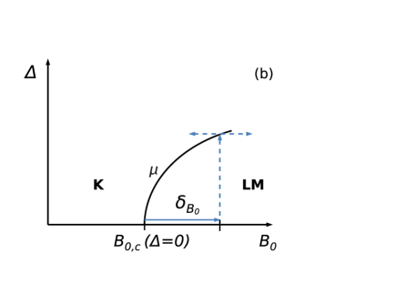
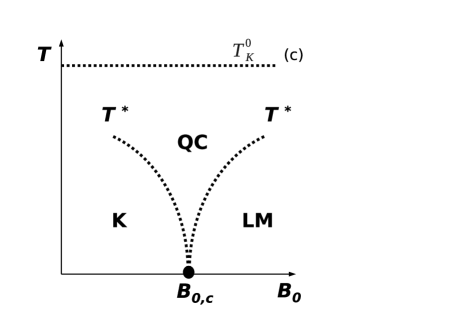
Figure 2: (Color online) (a) Schematic of the projected RG flows for the BFKM and the spin-boson model in a three-dimensional space spanned by the Kondo spin-flip coupling $J_{\perp}$, the bosonic coupling $B_{0}$, and the transverse field $\Delta$. (The flow of the longitudinal Kondo coupling $J_{z}$ is not shown.) Arrows on solid lines show the direction of RG flow and circles represent unstable fixed points. Arrows on dashed lines indicate the tuning of the bare couplings. (b) Schematic representation of the procedure of parameter tuning outlined in the text. (c) Schematic $B_{0}$-$T$ phase diagram for BFKM systems. The upper range of the quantum-critical (QC) regime is set by $T_{K}^{0}$, the Kondo temperature scale associated with the $B_{0}=0$ problem. The boundary between the LM and K phases as shown in (a) and (b) is parameterized by $\mathbf{\mu}=(B_{0,c},\Delta_{c}(B_{0,c}))$ for fixed $\rho_{0}J_{K}=0.5$.

This critical point governs the transition between the Kondo (K) phase and the Kondo-destroyed local-moment (LM) phase. A transverse field introduces spin flips into the impurity sector, thereby tending to disfavor the presence of a well-defined local moment. This leads one to consider whether there will be a quantum phase transition upon increasing $\Delta$ at fixed $J_{K}$ and $B_{0}$. To address this issue, it is instructive to recall that for $J_{K}=0$, the BFKM reduces to the spin-boson model (SBM), where increasing $\Delta$ is known to drive the system through a second-order quantum phase transition along a line in the $B_{0}$-$\Delta$ plane [see Fig. 2(a)]. It therefore seems highly probable for there to be a phase transition in the $B_{0}$-$\Delta$ plane at a fixed value $J_{\perp}>0$, as indicated by the dashed lines in Fig. 2(a). The expected behavior shown in Fig. 2(a) also suggests that at a fixed $\Delta>0$, one should still anticipate encountering a Kondo-destruction quantum phase transition as $B_{0}$ is increased. This, in turn, raises intriguing questions about the relation between any Kondo-destruction critical points reached for nonzero $\Delta$ and the $\Delta=0$ BFKM fixed point, and in particular about the evolution of the critical properties with $\Delta$.

II.3 Numerical renormalization-group method

For $\Delta=0$, the BFKM has been treated successfullyZhu:02 using an analytical renormalization-group procedure based on an expansion in $\epsilon=1-s$. It proves to be very difficult to account for a transverse magnetic field under this approach. By contrast, Eq. (1) can be solved for arbitrary values of $\Delta$ using the Bose-Fermi extensionGlossop:05+07 of the numerical renormalization group.Wilson:75 This section summarizes the Bose-Fermi NRG method and mentions a few details of its application to the present problem.

The key elements of the method are (i) the division of the continua of band and bath states into logarithmic bins spanning energy ranges $\Lambda^{-m+1}<\pm\epsilon/D,\>\omega/\omega_{0}<\Lambda^{-m}$ for $m=0$, $1$, $2$, $\ldots$, with $\Lambda>1$ being the Wilson discretization parameter, (ii) an approximation of all states within each bin by a single representative state, namely, the particular linear combination of states that couples to the impurity and, (iii) mapping of the problem via the Lanczos method onto a problem in which the impurity couples only to the end sites of two nearest-neighbor tight-binding chains, one fermionic and the other bosonic, having hopping coefficients and on-site energies that decay exponentially along each chain. These steps yield a Hamiltonian that can be expressed as the limit $H_{\text{BFKM}}=\lim_{N\to\infty}\alpha\Lambda^{-N/2}DH_{N}$ of an iterative sequence of dimensionless, scaled Hamiltonians

$$H_{N} =\Lambda^{1/2}H_{N-1}$$

$$+\frac{\Lambda^{N/2}}{\alpha}\biggl{\{}\sum_{\sigma}\Bigl{[}\epsilon_{N}f_{N\sigma}^{{\dagger}}f_{N\sigma}^{\phantom{{\dagger}}}+\tau_{N}\bigl{(}f_{N\sigma}^{{\dagger}}f_{N-1,\sigma}^{\phantom{{\dagger}}}+\text{H.c.}\bigr{)}\Bigr{]}$$

$$+\tilde{N}\,\frac{\omega_{0}}{D}\Bigl{[}e_{M}b_{M}^{{\dagger}}b_{M}^{\phantom{{\dagger}}}+t_{M}\bigl{(}b_{M}^{{\dagger}}b_{M-1}^{\phantom{{\dagger}}}+\text{H.c.}\bigr{)}\Bigr{]}\biggr{\}},$$ (4)

where $\alpha=\frac{1}{2}{\Lambda}^{{1}/{2}}\left(1+{\Lambda}^{-1}\right)$, $\tilde{N}=N\bmod 2$, and $M=N/2$. For the flat conduction-band density of states in Eq. (2), $\epsilon_{N}=0$ while $\tau_{N}\propto\Lambda^{-N/2}$ for $N\gg 1$, meaning that in Eq. (II.3) the combination $\Lambda^{N/2}\tau_{N}$ approaches $1$. By contrast, the bosonic tight-binding coefficients $e_{M}$ and $t_{M}$ both vary as $\Lambda^{-M}$ for $M\gg 1$. In order to treat similar fermionic and bosonic energy scales at the same stage of the calculation, one site is added to the end of the fermionic chain at each iteration, whereas the bosonic chain is extended by the addition of site $M$ only at even-numbered iteration $N=2M$. The iterative solution begins with the atomic limit described by $H_{0}$, where

$$\alpha H_{0} =\rho_{0}J_{0}\mathbf{S}\cdot\sum_{\sigma,\sigma^{\prime}}f_{0\sigma}^{{\dagger}}\bm{\sigma}_{\sigma,\sigma^{\prime}}f_{0\sigma^{\prime}}^{\phantom{{\dagger}}}+\sum_{\sigma}\epsilon_{0}f_{0\sigma}^{{\dagger}}f_{0\sigma}^{\phantom{{\dagger}}}$$ (5)

$$+\frac{\omega_{0}}{D}\biggl{[}\biggl{(}\frac{B_{0}}{\pi(s\!+\!1)}\biggr{)}^{1/2}\!\!S_{z}\bigl{(}b_{0}^{\phantom{{\dagger}}}+b_{0}^{{\dagger}}\bigr{)}+e_{0}b_{0}^{{\dagger}}b_{0}^{\phantom{{\dagger}}}\biggr{]}+\frac{\Delta}{D}\,S_{x}.$$

Many-body eigenstates of iteration $N-1$ are combined with basis states of fermionic chain site $N$ and (for $N=2M$) bosonic chain site $M$ to form a basis for iteration $N$. $H_{N}$ is diagonalized in this basis, and these eigenstates in turn are used to form a basis for iteration $N+1$. In order to maintain a basis of manageable dimension, only the $N_{s}$ eigenstates of lowest energy are retained after each iteration.Wilson:75 In Bose-Fermi problems,Glossop:05+07 one must also restrict the basis of each bosonic chain site to the $N_{b}+1$ number eigenstates $0\leq b_{M}^{{\dagger}}b_{N}^{{\dagger}}\leq N_{b}$. For further details, see Refs. Wilson:75, and Glossop:05+07, .

In the presence of a transverse magnetic field $\Delta$, no component of the total spin is conserved. However, $H_{N}$ commutes with the total “charge” operator

$$\hat{Q}=\sum_{n=0}^{N}\bigl{(}f_{n\uparrow}^{{\dagger}}f_{n\uparrow}^{\phantom{{\dagger}}}+f_{n\downarrow}^{{\dagger}}f_{n\downarrow}^{\phantom{{\dagger}}}-1\bigr{)},$$ (6)

Since the conduction-band density of states in Eq. (2) is particle-hole symmetric, $H_{N}$ also commutes with

$$\hat{I}_{+}=\sum_{n=0}^{N}(-1)^{n}f_{n\uparrow}^{{\dagger}}f_{n\downarrow}^{{\dagger}}$$ (7)

and its adjoint $\hat{I}_{-}=\hat{I}_{+}^{{\dagger}}$. In such cases, U(1) charge conservation symmetry is promoted to an SU(2) isospin symmetry with generators $\hat{I}_{\pm}$ and $\hat{I}_{z}=\frac{1}{2}\hat{Q}$. This symmetry ensures that the many-body eigenstates of $H_{N}$ can be labeled with quantum numbers $(I,Q)$ and may be grouped into multiplets of degeneracy $2I+1$. Moreover, it allows the NRG calculations to be performed using a reduced basis of states with $Q=-2I$. Our computations took advantage of these symmetry properties to reduce the labor of obtaining the eigensolution.

Throughout the remainder of this paper, all energies are expressed as multiples of the half-bandwidth $D=1$. The NRG results presented in the next section were all obtained for bath exponent $s=0.8$ and dimensionless Kondo coupling $\rho_{0}J=0.5$. All calculations were performed using a Wilson discretization parameter $\Lambda=9$, allowing up to $N_{b}=8$ bosons per site, and retaining up to $N_{s}=500$ isospin multiplets after each iteration; all values that were shown in Ref. Glossop:05+07, yield reliable results for the BFKM without any transverse field.

III Kondo-Destruction Quantum Phase Transition

In this section, we determine the phase diagram of the Ising-anisotropic BFKM in the presence of a local transverse field. We focus attention on the Kondo-destruction quantum phase transition, which separates a Kondo (K) phase and a Kondo-destroyed local-moment (LM) phase.

III.1 Critical Kondo Destruction

We began by locating the quantum phase transition of the BFKM in the absence of a transverse field, expressed as a critical coupling to the bosonic bath $B_{0,c}(\Delta\!=\!0)$ (for the fixed value $\rho_{0}J_{K}=0.5$ used throughout this work). The signature of proximity to a critical point is the flow of the NRG many-body eigenenergies over some finite range of intermediate iterations $N$ (corresponding to a window of temperatures $T\sim\Lambda^{-N/2}$) to new values distinct from the converged eigenenergies obtained for large $N$. The latter spectra describe the stable RG fixed points of the problem, which in this case govern the K and LM phases. As $B_{0}$ is tuned closer to $B_{0,c}(\Delta\!=\!0)$, the energies remain flat and close to the new values over an increasingly wide range of $N$.

Once $B_{0,c}(\Delta\!=\!0)$ was determined, we considered a sequence of five larger bosonic couplings

$$B_{0}=B_{0,c}(\Delta\!=\!0)+\delta_{B_{0}},$$ (8)

where $\delta_{B_{0}}=6\times 10^{-n}$ with $n=1,\ldots,5$. For each value of $\delta_{B_{0}}$, we increased the transverse field from zero until we reached a new critical point, again judged by examination of the many-body spectrum. Once the critical field $\Delta_{c}(\delta_{B_{0}})$ was established, we fixed $\Delta=\Delta_{c}$ and tuned $B_{0}$ around the value $B_{0,c}(\Delta_{c})\equiv B_{0,c}(0)+\delta_{B_{0}}$ in order to calculate the critical properties associated with the finite-$\Delta$ transition. The procedure is illustrated schematically in Fig. 2(b).

Since all values of $\delta_{B_{0}}$ show qualitatively the same behavior, we concentrate below on the representative case ${\delta}_{B_{0}}=6\times{10}^{-3}$. The charge $Q$ defined in Eq. (6) is a good quantum number, so it can be used to label the different NRG many-body eigenstates. To begin with, we consider states having $Q=0$. (The $Q=1$ states are discussed in detail in Sec. IV.) Figure  3 shows the energy of the lowest excited $Q=0$ state as a function of iteration number for $\delta_{B_{0}}=6\times{10}^{-3}$. The spectrum is different for odd $N$, not only due to the alternation properties of fermions on finite tight-binding chains, but also because bosons are added only at even iterations.Glossop:05+07 Since the many-body ground state shares the quantum number $Q=0$, we provisionally interpret the lowest excited state of the same charge as having bosonic character.

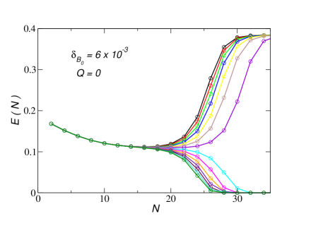
Figure 3: The lowest bosonic ($Q=0$) eigenenergy as a function of even iteration number for $\delta_{B_{0}}=6\times{10}^{-3}$. The energies converging to $E\ \simeq 0.39$ correspond to effective bosonic couplings $-9.45\times 10^{-6}\leq B_{0}-B_{0,c}\leq-8.5\times 10^{-7}$, while the energies converging to $E=0$ span the range $8.5\times 10^{-7}\leq B_{0}-B_{0,c}\leq 9.45\times 10^{-6}$.

From Fig. 3, one can clearly distinguish the quantum-critical regime at intermediate values of $N$ and the crossover for large $N$ to either the K or the fixed LM point. For $B_{0}<B_{0,c}$, the first bosonic excitation energy eventually approaches the value $E\simeq 0.39$ that it takes in the free-boson spectrum obtained for $B_{0}=0$. For $B_{0}>B_{0,c}$, the first bosonic excitation energy eventually vanishes, reflecting the two-fold degeneracy of the ground state in the LM phase. In the quantum-critical regime, the excitation energy takes a distinct value $E\simeq 0.11$ that can be considered a characteristic of the QCP.

The crossover to the spectrum of either the LM or the K fixed point can be used to estimate the crossover scale $T^{*}\sim\Lambda^{-N^{*}/2}$, where $N^{*}$ is the iteration at which the difference of the eigenvalues from their critical values exceeds a predetermined threshold. The lowest bosonic eigenvalue in Fig. 3 shows that $T^{*}$ vanishes at the critical point from both sides since $N^{*}\to\infty$ as $B_{0}\to B^{\pm}_{0,c}$. The schematic $B_{0}$-$T$ phase diagram is shown in Fig. 2(c).

The local magnetization, defined as

$$M_{z}=\mathop{\lim}_{h\to 0,\ T\to 0}\left\langle S_{z}\right\rangle$$ (9)

where $h$ is a longitudinal magnetic field, is nonzero in the LM phase, vanishes continuously as $B_{0}\to B^{+}_{0,c}$, and remains zero throughout the K phase, as shown in Fig. 4(a).

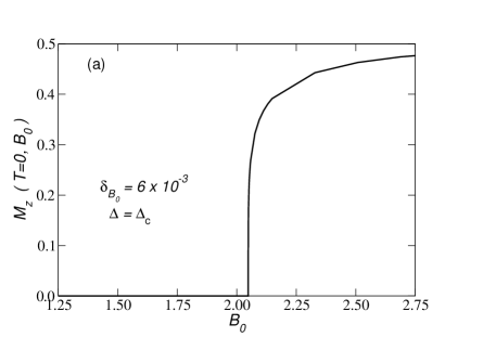
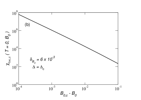
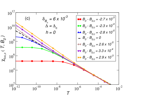
Figure 4: (a) Local magnetization $M_{z}$ vs $B_{0}$ across the quantum phase transition. (b) Zero-temperature longitudinal susceptibility $\chi_{\mathrm{loc},z}$ in the Kondo phase near the critical point. (c) $\chi_{\mathrm{loc},z}$ vs $T$ for $B_{0}$ values at (dashed line) and near (symbols) $B_{0,c}$. All data are for $\delta_{B_{0}}=6\times 10^{-3}$.

III.2 Critical Exponents

The local susceptibility in the $z$-direction defined as

$$\chi_{loc,z}\left(T;\omega=0\right)=-{\left.\frac{\partial\left\langle S_{z}\right\rangle}{\partial h}\right|}_{h=0}={\mathop{\lim}_{h\to 0}\left(-\frac{\left\langle S_{z}\right\rangle}{h}\right)\ }$$ (10)

diverges at $T=0$, $B_{0}\to B^{-}_{0,c}$ as shown in Fig. 4(b).

The distinctions between the LM, K and QC regimes [see Fig. 2(c)] can also be seen by analyzing $\chi_{loc,z}(B_{0},T)$ in the corresponding regimes. Figure 4(c) shows $\chi_{loc,z}(B_{0},T)$ for values of $B_{0}$ below, above and close to $B_{0,c}$. For $T>T^{*}$, flows from both $B_{0}<B_{0,c}$ and $B_{0}>B_{0,c}$ behave the same way by scaling as $T^{-x}$, while for $T<T^{*}$, the K fixed point is characterized by a constant Pauli susceptibility and the LM fixed point susceptibility follows a $1/T$ Curie-Weiss form.

We have extracted critical exponents for all five investigated values. The crossover scale $T^{*}$ vanishes from both the LM and K phases as

$$T^{*}\propto{\left|B_{0}-B_{0,c}\right|}^{\nu z}$$ (11)

with $z=1$ for an impurity problem. $T^{*}$ was estimated from the crossover iteration number $N^{*}$ as explained in Sec. III.A. Figures 5(a) and 5(b) show the scaling of $T^{*}$ with distance from $B_{0,c}\$from the K and LM sides, respectively. It is apparent that for all values of ${\delta}_{B_{0}}$ considered, $\nu$ is essentially the same.

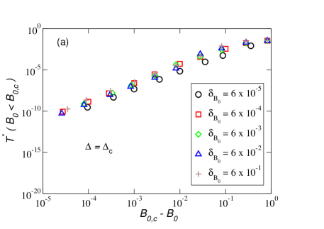
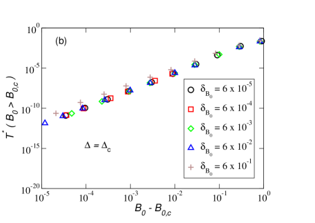
Figure 5: Scaling of $T^{*}$ with $B_{0}$ on the K side (a) and on the LM side (b) of the QCP.

It is found that $M_{z}(T=0)$ decays as a power law on the LM side:

$$M_{z}(h\to 0,T\to 0,\ \Delta\to{\Delta}_{c})\propto{\left(B_{0}-B_{0,c}\right)}^{\beta},$$ (12)

where $h\$is an infinitesimal field applied along the $z$ direction as can be seen in Fig. 6(a) for all ${\delta}_{B_{0}}$. It also scales with $h$ at $B_{0}\simeq B_{0,c}$:

$$M_{z}(h,\ B_{0}=B_{0,c},T=0)\ \propto{\left|h\right|}^{1/\delta}.$$ (13)

This is shown in Fig. 6(b) for all ${\delta}_{B_{0}}$increments.

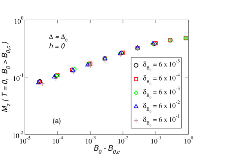
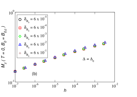
Figure 6: (a) Scaling of $M_{z}$ with $B_{0}$ from LM side. (b) Scaling of $M$ with $h$ at $B_{0}=B_{0,c}$.

The local susceptibility in the $z$ direction diverges on approach to the QCP from the K side at $T=0$:

$${{\rm\chi}}_{loc,z}(B_{0}<B_{0,c},T=0)\propto{\left(B_{0,c}-B_{0}\right)}^{-\gamma}$$ (14)

and scales with temperature as

$${{\rm\chi}}_{loc,z}(B_{0}=B_{0,c},T>T^{*}\ )\propto T^{-x},$$ (15)

as illustrated in Figs. 7(a) and 7(b) respectively.

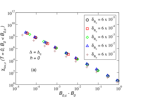
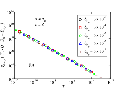
Figure 7: (a) Scaling of ${{\rm\chi}}_{loc,z}$ with $B_{0}$ on the K side of the QCP. (b) Scaling of $\chi_{loc,z}$ with $T$ at $B_{0}=B_{0,c}$.

The values of all the calculated critical exponents for all values of ${\delta}_{B_{0}}$ are shown in Fig. 8. The parameter $\mathbf{\mu}=(B_{0,c},\Delta_{c}(B_{0,c}))$ defines the boundary between the LM and K phases for fixed $\rho_{0}J_{K}=0.5$ as shown in Figs. 2(a) and 2(b).

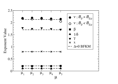
Figure 8: Calculated critical exponents. The exponents at the critical coupling $\Delta_{c}$ corresponding to different choices of $\delta_{B_{0}}$ and for fixed $\rho_{0}J_{K}=0.5$ as illustrated in Figs. 2(a) and 2(b). The ordinate $\mu_{1}$ corresponds to $\delta_{B_{0}}=6\times 10^{-5}$, $\mu_{2}$ to $\delta_{B_{0}}=6\times 10^{-4}$, and so on. The dashed lines show the corresponding exponents for the $\Delta=0$ BFKM, with $x$ and $\beta$ being NRG results and the remaining exponents derived assuming hyperscaling.

We note that the critical exponents are virtually the same as those for the $\Delta=0$ BFKM, indicated using dashed lines in Fig. 8. It was previously foundGlossop:05+07 that the exponents obey the hyperscaling relations derived from the ansatz

$$F_{crit}=Tf\left(\frac{\left|\Delta-{\Delta}_{c}\right|}{T^{1/\nu}},\ \frac{\left|h\right|}{T^{b}}\right),$$ (16)

namely

$$\delta=\frac{1+x}{1-x},$$ (17)

$$\beta=\frac{1}{2}\nu\left(1-x\right),$$ (18)

$$\gamma=\nu x$$ (19)

Since the $\Delta>0$ critical exponents coincide for all the values of $\delta_{B_{0}}$ with their $\Delta=0$ counterparts, hyperscaling also holds in the presence of a transverse field.

We also stress that these conclusions are restricted to the case of bath exponent $s=0.8$ treated in this paper. Studies for other values of $s$ will be reported elsewhere.

The error estimates and other related issues are discussed in the Appendix.

IV Line of Kondo-destruction fixed points

Having established the existence of Kondo-destruction transitions in the presence of a transverse local magnetic field $\Delta$, we turn next to the relationship among the critical points for different values of $\Delta$.

One possibility is that the RG flows are away from the $\Delta{\rm=0\ }$BFKM critical fixed point towards a different unstable fixed point, which effectively governs the transitions for all the ${\delta}_{B_{0}}$considered.

A plausible conjecture is that these flows take the system from the critical fixed point of the $\Delta=0$ BFKM to the critical fixed point of the SBM [See Fig. 2(a)]. The true asymptotic critical behavior will be that associated with the SBM model, where the transverse field is solely responsible for quantum-mechanical tunneling with a critical suppression of Kondo tunneling (${\rho J}^{*}_{\bot}=0)$. Other related scenarios are of course possible a priori.

A second possibility is that there is a line of unstable fixed points extending from the original $\Delta{\rm=0\ }$BFKM. In this case, we expect that each of the trial ${\delta}_{B_{0}}$ is tuned to its own unstable fixed point. We believe this is the correct picture.

An indication in favor of the second possibility comes from the critical many-body NRG spectrum extracted from the flows on the verge of crossing over to either stable fixed point. The many-body spectrum can be decomposed into a superposition of distinct fermionic and bosonic excitations at any of the two stable fixed points.Glossop:05+07 Here, the lowest $Q=1$ excitations correspond to single-particle charged fermionic excitations, while the lowest $Q=0$ excitations are single boson excitations. Note also that in both of the above cases, one can have higher energy charge $0$ particle-hole excitations. The excitation energy can be written as $E_{Exc}=E_{Fermion}+E_{Boson}$. At the LM fixed point $E_{Boson}$ consists of a superposition of free-boson excitations, while $E_{Fermion}$ is an energy from the spectrum of fermions undergoing spin-dependent potential scattering. At the K fixed point, $E_{Boson}$ is given by free-boson excitations and $E_{Fermion}$ is the energy of one or more Kondo-like quasiparticles. Such a sharp distinction cannot be established rigorously from the flows close to the critical point.

The flows for the lowest six states closest to the critical point for ${\delta}_{B_{0}}=6\times{10}^{-3\ }$are shown in Fig. 9 for $Q=1$.

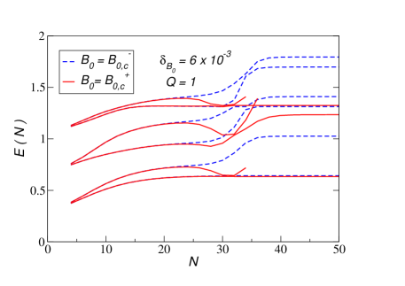
Figure 9: Eigenenergy $E$ vs iteration number $N$ for the six lowest $Q=1$ states near the critical couplings for $\delta_{B_{0}}=6\times 10^{-3}$, showing flow away from the critical spectrum to the LM (solid) and K (dashed) sides.

The figure shows the flows for values of the coupling slightly below, and above the critical point. For $B_{0}<\ B_{0,c}$ the flows approach a plateau characteristic of the slow variation close to the unstable fixed point and eventually move away to the K fixed point. For $B_{0}>\ B_{0,c}$ we see the same critical values, which then move towards the LM fixed point. Notice that in this latter regime the states tend to become doubly degenerate and can be fitted to a spin-dependent potential scattering term corresponding to a finite ${\rho J}^{*}_{z}\$term. This is also consistent with the full suppression of any tunneling term. Half of the flows tend to diverge quickly beyond $N\simeq 34$ and are truncated in the figure. This lifting of the degeneracy is a purely numerical artifact in the LM regime and we do not expect it to have any significant bearing on our conclusions. In the critical regime, $N\simeq 24$ , the $Q=1$ states show a splitting due to an effective finite ${\Delta}^{*}\$term which is absent in the $\Delta{\rm=0}$ BFKM case. Formally, a nonzero bare $\Delta$ implies that the total spin projection along the z-axis is not conserved. To see all this we show the lowest six estimated $Q=1$ critical eigenvalues ($N\simeq 24$) for all ${\delta}_{B_{0}}$ trials in Fig. 10.

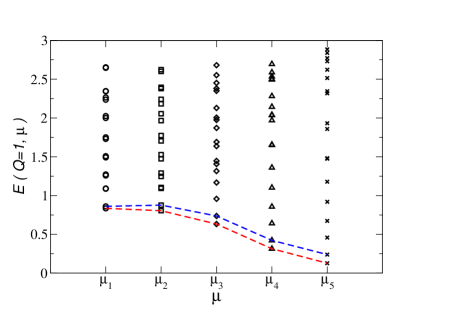
Figure 10: Lowest $Q=1$ eigenvalues closest to the critical point ($N\simeq 24)$ for each case $\mu_{1}$ to $\mu_{5}$ defined in the caption of Fig. 8. The dashed lines track the evolution of the splitting between the two lowest states.

In Figs. 8, 10, and  12, $\mu_{1}$ corresponds to the critical couplings found for $\delta_{B_{0}}=6\times 10^{-5}$, $\mu_{2}$ to that for $\delta_{B_{0}}=6\times 10^{-4}$ and so on. Referring to the lowest two values in Fig. 10, one can clearly see that the splitting increases continuously with ${\delta}_{B_{0}\ }$. For higher states, it becomes very difficult to follow the trend due to possible level crossings.

The $Q=0$ flows are shown in Fig. 11 for $B_{0}$ around $B_{0,c}$. It is well known Weiss:1999 ; 41 that the truncation of the bosonic Hilbert space results in improperly converged boson eigenvalues at the LM fixed point. However, NRG truncation does not affect the critical bosonic spectrum. Figure 12 shows the estimates for the lowest few $Q=0$ critical eigenvalues. One sees that some of these critical flows do not change with ${\delta}_{B_{0}}$. For the rest, it is more difficult to determine if the eigenvalues are indeed changing continuously as in the $Q=1$ sector. It is possible that the $Q=0$ eigenvalues which are changing are those associated with the fermionic excitation, while the constant values correspond to an unchanging purely bosonic sector.

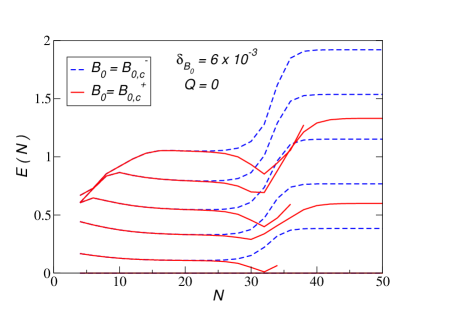
Figure 11: Eigenenergy $E$ vs iteration number $N$ for the six lowest $Q=0$ states near the critical couplings for $\delta_{B_{0}}=6\times 10^{-3}$, showing flow away from the critical spectrum to the LM (solid) and K (dashed) sides.

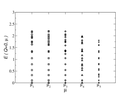
Figure 12: Lowest $Q=0$ eigenvalues closest to the critical point ($N\simeq 24$) for each case $\mu_{1}$ to $\mu_{5}$ defined in the caption of Fig. 8.

Although it is difficult at this stage to make strong statements about the nature of these critical excitations we can attest at least to the fact that in the $Q=1$ case they appear to change continuously with ${\delta}_{B_{0}}$. A reasonable scenario is that the extra dissipation provided by increased ${\delta}_{B_{0}}$ requires an increased renormalized effective ${\Delta}^{*}$ at the critical point. Some evidence for this is also provided since one requires an increasing bare ${\Delta}_{c}$ with increasing ${\delta}_{B_{0}}$ in order to bring the flows closer to the critical surface. The fact that the spectrum changes provides evidence that we are dealing with a line of unstable fixed points extending from the $\Delta{\rm=0}$ BFKM and having the same set of critical exponents as the former. In the alternate scenario alluded to above, a flow to a different unstable fixed point would produce essentially the same critical eigenvalues for all ${\delta}_{B_{0}}\$cases. A schematic flow diagram for the transverse-field BFKM showing a line of critical fixed points extending from the $\Delta{\rm=0}$ case is given in Fig. 13.

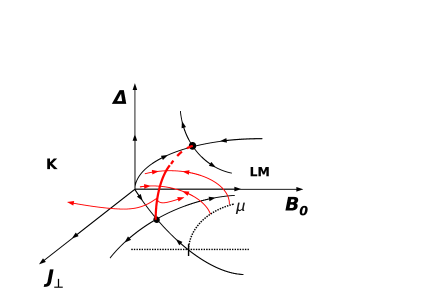
Figure 13: Schematic flow diagram showing a line of unstable fixed points extending from the $\Delta{\rm=0}$ BFKM critical fixed point with a conjectured extension (dashed) to the the SBM critical point lying on the plane $J_{\perp}=0$.

We stress that the many-body spectrum of the unstable fixed point reflects the universal properties of the critical point. Because of the non zero transverse field applied along the $x$ direction, a magnetization will be generated that is directed along the $x$ direction, as considered, e.g. in Ref. 41, in the SBM; this magnetization does not contain any critical singularity. Nonetheless, the end result of tuning $\Delta$ is to make the many-body spectra of the unstable fixed points vary continuously, which is captured by the line of fixed points shown in Fig. 13.

We close this section by noting that the $Q=1$ eigenstates in the K phase do not recover the $SU(2)$ symmetry characteristic of a simple Kondo singlet suggesting that there is a residual splitting due to the transverse field. As shown in Fig. 9, these splittings are larger in the converged K phase eigenvalues than in the critical regime suggesting that the effective $\Delta$ increases with flows away from the critical points. At the same time, the $Q=1$ eigenvalues for $B_{0}>B_{0,c}$ recover the two fold degeneracy typical of the LM fixed point with vanishing tunneling amplitude $\Delta^{*}$ in all of the $\delta_{B_{0}}$ cases considered.

V Conclusions

We have carried out numerical renormalization-group studies of the Bose-Fermi Kondo model in the presence of a transverse field $\Delta$ for different values of the coupling to a dissipative bosonic bath with a bath exponent $s{\rm=}{\rm 0.8}$. We found that the system can be tuned across a second-order quantum phase transition between a local-moment phase and a Kondo screened phase. We also found that the transition is characterized by critical exponents identical to those of the $\Delta{\rm=0\ }$BFKM for $s{\rm=}{\rm 0.8}$, and exhibits hyperscaling. A continuously varying critical spectrum suggests that these new fixed points are lying on a line of critical fixed points extending from the known $\Delta{\rm=0\ }$BFKM critical point.

Our results are interesting in their own right. Furthermore, in the Ising-anisotropic Kondo lattice model, a transverse field introduces quantum fluctuations in the local-moment component. Through the extended dynamical mean field theory, a self-consistent Bose-Fermi Kondo model with Ising anisotropy and a transverse local field provides the means to study the Ising-anisotropic Kondo lattice model with a transverse field. The results reported here will therefore have implications for the Kondo-destruction transitions in the lattice model. In particular, our evidence for the line of unstable fixed points in the Bose-Fermi Kondo model suggests a line of Kondo-destruction quantum critical point in the lattice model, as in the proposed global phase diagram. Concrete studies of the lattice model will be undertaken in the future.

Appendix A Accuracy in the determination of the critical exponents

As a check on our estimates of critical exponents obtained by varying $B_{0}$ around $B_{0,c}$ at fixed $\Delta=\Delta_{c}$, we have also calculated these exponents by fixing $B_{0}=B_{0,c}$ and then tuning $\Delta$ through $\Delta_{c}$. Figure 14 compares the exponents obtained via these two methods, in each case retaining 500 isospin multiplets in the NRG calculations.

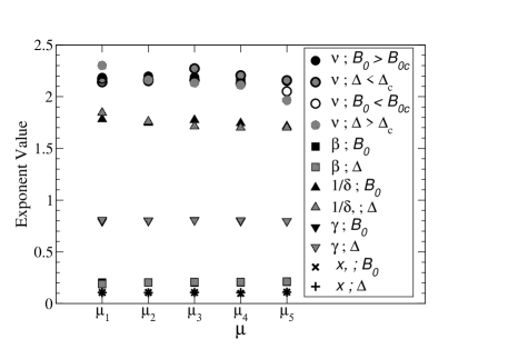
Figure 14: Comparison of critical exponents obtained by tuning through the critical point by varying $B_{0}$ and by varying $\Delta$, showing results for each case $\mu_{1}$ to $\mu_{5}$ defined in the caption of Fig. 8.

There is some mismatch between the estimated exponents for the $\Delta$ and $B_{0}$ tuning cases. This is especially pronounced for ${\nu}_{LM}$ and ${\nu}_{K}$ with the smallest and largest ${\delta}_{B_{0}}$ corresponding to cases $\mu_{1}$ and $\mu_{5}$, respectively, in Fig. 14.

The discrepancies in the first case may be attributable to a vanishing $\Delta^{*}$ at the unstable fixed point parameterized by $\mu_{1}$. For small changes in the bare $\Delta$ close to ${\Delta}_{c}\$ the change to the RG flow is particularly small due to proximity to the critical point, making it difficult to accurately determine the scaling property.

The second, larger discrepancy in $\nu$ is noticed for $\mu_{5}$. We observe in this case that the many-body eigenvalues approach the critical plateau at higher-numbered iterations and leave this vicinity sooner than all the other cases considered. This suggests that the flows do not come as close to an unstable fixed point as in the other cases.

Excluding these sources of error, it is clear that the exponents found by tuning $\Delta$ are the same as those found by tuning $B_{0}$.

The error in the critical exponents is estimated to be of ${\rm O}\left({10}^{-1}\right)$ for $\nu$  which was determined from the eigenvalue flows and of$\ {\rm O}({10}^{-2}$) for the thermodynamic critical exponents.

References

- (1) Q. Si and F. Steglich, Science, 329, 1161 (2010).
- (2) G. R. Stewart, Rev. Mod. Phys, 73, 797 (2001).
- (3) P. Gegenwart, Q. Si and F. Steglich, Nature Phys., 4, 186 (2008).
- (4) H. v. Löhneysen, A. Rosch, M. Vojta, and P. Wölfle, Rev. Mod. Phys. 79 1015 (2007).
- (5) J. A. Hertz, Phys. Rev. B 14, 1165 (1976); A. J. Millis, ibid. 48, 7183 (1993) ; T. Moriya, Spin Fluctuations in Itinerant Electron Magnetism (Springer, Berlin, 1985).
- (6) Q. Si, S. Rabello, K. Ingersent and J. L. Smith, Nature (London) 413, 804 (2001).
- (7) Q. Si, S. Rabello, K. Ingersent and J. L. Smith, Phys. Rev. B 68, 115103 (2003).
- (8) P. Coleman, C. Pepin, Q. Si and R. Ramazashvili, J. Phys. Condens. Matter 13, R723 (2001).
- (9) J. L. Smith and Q. Si, Phys. Rev. B 61, 5184 (2000); Q. Si and J. L. Smith, Phys. Rev. Lett. 77, 3391 (1996).
- (10) R. Chitra and G. Kotliar, Phys. Rev. Lett. 84, 3678 (2000).
- (11) S. Paschen,T. Lühmann, S. Wirth, P. Gegenwart, O. Trovarelli, C. Geibel, F. Steglich, P. Coleman, and Q. Si, Nature (London) 432, 881 (2004).
- (12) S. Friedemann, N. Oeschler, S. Wirth, C. Krellner, C. Geibel, F. Steglich, S. Paschen, S. Kirchner, and Q. Si, Proc. Natl. Acad. Sci. U.S.A. 107, 14547 (2010).
- (13) H. Shishido, R. Settai, H. Harima, and Y. Ōnuki, J. Phys. Soc. Jpn. 74, 1103 (2005).
- (14) A. Schroeder, G. Aeppli, R. Coldea, M. Adams, O. Stockert, H. v. Lohneysen, E. Bucher, R. Ramazshvili, and P. Coleman, Nature (London) 407, 351 (2000).
- (15) D. R. Grempel and Q. Si, Phys. Rev. Lett. 91, 026401 (2003).
- (16) J.-X. Zhu, D. R. Grempel, and Q. Si, Phys. Rev. Lett. 91, 156404 (2003).
- (17) M. T. Glossop and K. Ingersent, Phys. Rev. Lett. 99, 227203 (2007).
- (18) J. X. Zhu, S. Kirchner, R. Bulla, and Q. Si, Phys. Rev. Lett. 99, 227204 (2007).
- (19) Q. Si, Phys. Status Solidi B 247, 476 (2010); Physica B 378, 23 (2006).
- (20) S. Friedmann, T. Westerkamp, M. Brando, N. Oeschler, S. Wirth, P. Gegenwart, C. Krellner, C. Geibel and F. Steglich, Nat. Phys. B, 465 (2009).
- (21) J. Custers, P. Gegenwart, C. Geibel, F. Steglich, P. Coleman, and S. Paschen, Phys. Rev. Lett. 104, 186403 (2010).
- (22) S. L. Bud’ko, E. Morosan, and P. C. Canfield, Phys. Rev. B 71, 054408 (2005).
- (23) J. Custers et al., Nat. Mater. 11, 189 (2012).
- (24) M. S. Kim and M. C. Aronson, Phys. Rev. Lett. 110, 017201 (2013).
- (25) E. D. Mun et al., Phys. Rev. B 87, 075120 (2013).
- (26) V. Fritsch et al., arXiv:1301.6062.
- (27) D. D. Khalyavin et al., Phys. Rev. B 87, 220406(R) (2013).
- (28) L. Zhu and Q. Si, Phys. Rev. B 66, 024426 (2002).
- (29) G. Zaránd and E. Demler, Phys. Rev. B 66, 024427 (2002).
- (30) M. T. Glossop, and K. Ingersent, Phys. Rev. Lett. 95, 067202 (2005); Phys. Rev. B 75, 104410 (2007).
- (31) A. J. Leggett, S. Chakravarty, A. T. Dorsey, M. P. A. Fisher, A. Garg, and W. Zwerger, Rev. Mod. Phys. 59, 1 (1987).
- (32) K. G. Wilson, Rev. Mod. Phys. 47, 773 (1975).
- (33) R. Bulla, H. J. Lee, N. H. Tong, and M. Vojta, Phys. Rev. B 71, 045121 (2005); R. Bulla, N. H. Tong, and M. Vojta, Phys. Rev. Lett. 91, 170601 (2003).
- (34) U. Weiss, Quantum Dissipative Systems (World Scientifc, Singapore, 1999).
- (35) K. Le Hur, Ann. Phys. (N.Y.) 323, 2208 (2008).