Efficient Algorithms for
Universal Quantum Simulation

Abstract

A universal quantum simulator would enable efficient simulation of quantum dynamics by implementing quantum-simulation algorithms on a quantum computer. Specifically the quantum simulator would efficiently generate qubit-string states that closely approximate physical states obtained from a broad class of dynamical evolutions. I provide an overview of theoretical research into universal quantum simulators and the strategies for minimizing computational space and time costs. Applications to simulating many-body quantum simulation and solving linear equations are discussed

1 Introduction

A quantum computer could allow some problems to be solved more efficiently, by enabling efficient execution of quantum algorithms, as compared to executing classical algorithms on a classical computer that are inferior for those problems [1]. The “classical computer” refers to a computer that is built strictly according to the principles of classical physics but more specifically is equivalent to a Turing machine [2]. The subtle issues of a quantized computer operating over real rather than binary fields are not discussed here [3]. The study of “quantum simulation” focuses on simulating properties and dynamics of quantum systems whether by classical or quantum computation, and the topic of “efficient algorithms for quantum simulation” focuses on quantum simulation problems that do not have efficient classical algorithms.

Let me clear about terminology employed here. By the term simulation, I mean that certain pre-specified properties of the quantum system are accurately predicted by the simulation but not necessarily all properties. Accuracy refers to each answer being no worse than some error tolerance $\epsilon$. For example one might wish to know the mean momentum, the standard deviation of the momentum, and average energy. The simulation is successful if these quantities are accurately predicted by the simulator even if other irrelevant quantities are poorly predicted. The term efficiency refers to the simulation yielding an accurate solution to the problem with a resource (e.g., run-time and space usage) cost that increases no faster than a polynomial function of the input bit string and of $1/\epsilon$.

Explicitly defining simulation is important because various notions of quantum simulation using quantum computers, either purpose-built or universal, with various terminology. The term “digital quantum simulator” is sometimes employed to refer to a programmable quantum simulator, and the term “analogue quantum simulator” refers to a quantum system designed to behave analogously to a the quantum system being studied [4], and usually these terms are employed when error correction is not assumed hence making these systems not scalable. Analogue quantum simulation is sometimes called “quantum emulation” [5]. Our term “universal quantum simulator” is in concordance with “digital quantum simulator” provided that the latter uses a fault tolerant architecture as we assume simulation on a scalable quantum computer.

Quantum simulation can deal with non-relativistic single-particle quantum mechanics described by Schrödinger’s equation

$${\rm i}\frac{\rm d}{{\rm d}t}|\psi(t)\rangle=\hat{H}(t)|\psi(t)\rangle$$ (1)

with self-adjointness $\hat{H}=\hat{H}^{\dagger}$ implying unitary dynamics, but self-adjointness is not necessary. Alternatively simulation of relativistic quantum mechanics or many-body quantum dynamics [6] or quantum field theories [7] may be sought. For simplicity we focus on the easiest case of single-body dynamics (1) and thence to the many-body case.

After choosing the equation to be studied, the question then arises as to which problem is to be solved. Two possible problems include solving the state $|\psi(t)\rangle$ over some time domain or determining the spectrum of the Hamiltonian $\hat{H}$. Instead of finding the spectrum or some aspect of the spectrum such as the smallest or largest spectral gap, the problem could be about finding eigenvectors of $\hat{H}$ such as the ground state. For simulation purposes a natural question would be to estimate the expectation values of some observable

$$\langle\psi(t)|\hat{\mathcal{O}}|\psi(t)\rangle.$$ (2)

Some of the problems discussed here could be tractable on a classical computer hence making quantum algorithms uninteresting; other problems such as finding ground states could be intractable as well on a quantum computer [8].

2 Algorithms and complexity for quantum simulation

For algorithmic quantum simulation we are interested in those problems that are intractable on a classical computer yet tractable on a quantum computer. We can rule out solving problems that are amenable to the usual classical methods such as the following [9]. One approach is to diagonalize the Hamiltonian directly, which is always possible in principle but, as the problem size is polylogarithmic in dimension and diagonalization is polynomially expensive with respect to dimension, the cost of diagonalization is thus superpolynomially expensive hence is not efficient in general.

Another approach to quantum simulation is to integrate the dynamical equation, for example Schrödinger’s equation (1), directly. For example the Runge-Kutta technique is popular. Alternatively the dynamics can be tackled by constructing the evolution operator and using the Magnus, or Baker-Campbell-Hausdorff method, expansion. Product formulæ  are valuable as a unitary evolution can be factorized into an approximate product of unitary evolutions. Product formulæ  include the Forest-Ruth or symplectic integration, method, and the Trotter-Suzuki expansion is also valuable, especially for quantum simulation as we shall see.

Quantum Monte Carlo simulations include stochastic Green functions techniques and variational, diffusion or path-integral Monte-Carlo methods. Density matrix renormalization group techniques have become popular especially for one-dimensional many-body systems with slowly increasing entanglement with respect to the number of particles.

Perhaps the best insight into quantum simulation can be gained by studying Feynman’s own words in his seminal 1982 paper on quantum computing based on a his keynote talk on the topic “Simulating Physics With Computers” [10]. Feynman asks,

Can a quantum system be probabilistically simulated by a classical (probabilistic, I’d assume) universal computer? In other words, a computer which will give the same probabilities as the quantum system does. If you take the computer to be the classical kind I’ve described so far, (not the quantum kind described in the last section) and there’re no changes in any laws, and there’s no hocus-pocus, the answer is certainly, No! This is called the hidden-variable problem: it is impossible to represent the results of quantum mechanics with a classical universal device.

The concept of quantum simulation can be understood from the schematic in Fig. 1.

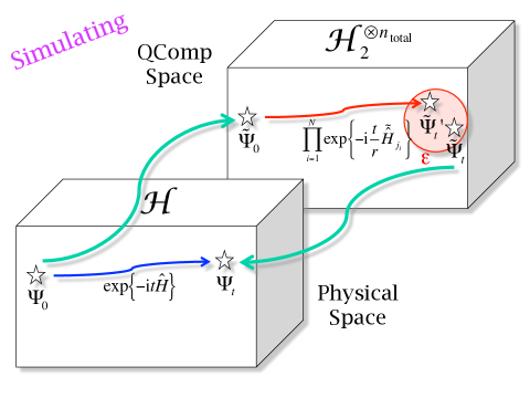
Figure 1: Quantum simulation is depicted by showing evolution of a state $\Psi_{0}$ in a Hilbert space $\mathcal{H}$ for the Physical Space and the evolution of the state’s approximation $\tilde{\Psi}_{0}$ in the $n$-qubit space $\mathcal{H}_{2}^{n}$ in the quantum computer, or QComp Space. In the physical world, the evolution is given by $\exp\{-{\rm i}t\hat{H}\}$ for $\hat{H}$ the system Hamilttonian and $t$ the time of evolution. The resultant state is $\Psi_{t}$. In the quantum computer, all information is restricted to finite bit strings and all quantum information to finite qubit strings so even continuous time $t$ is broken up into discrete intervals of duration $t/r$ and the Hamiltonian matrix is approximated by $\tilde{\hat{H}}$. The resultant simulated state is $\tilde{\Psi}^{\prime}_{t}$, which is different from the approximation of the true state $\tilde{\Psi}_{t}$ by less than a distance $\epsilon$.

The essence of this figure, which is fully explained in the caption, is that the quantum simulation necessarily approximates all information and quantum information into bit strings and qubit strings and delivers an approximation to the final state as a finite qubit string.

Let us now perform exegesis on Feynman’s words to seek an understanding of what he meant. In order to understand his meaning, we delve into computer science notions of complexity, not something that Feynman himself used. Thus, we seek to interpret a statement more than three decades old through the lens of modern computational complexity theory.

To understand, we cast quantum simulation as a decision problem: the computational problem is constructed so that the answer can only be Yes or No. To assess whether the quantum simulation is efficient, the question is then how hard, i.e., how do the computational resources scale with problem size expressed as the number of bits $n$ required to specify the input state, in order to answer the question? Note that the resources to prove Yes or No can differ, which leads to complexity classes and their complements. We are especially interested in the time and space costs, which we denote as $T$ and $S$, respectively.

Quantum simulation problems are no worse then EXP, which is the class of problems that can be solved with $T$ and $S$ increasing no more than an exponential function of $n$. That EXP is the worst case follows from using the Heisenberg matrix representation for the dynamics and seeing that the size of the register and the computational time for matrix operations leads to decision problems being in EXP.

Aaronson points out that Feynman (inadvertently) reduced the complexity of quantum mechanics to PSPACE; i.e., $S$ increases no more than polynomially in $n$ by introducing path integrals [11]. The class of decision problems solvable efficiently on a quantum computer is BQP, which refers to bounded-error quantum polynomial and is inside PSPACE. The aim of quantum simulation thus needs to focus on narrower problems than those in PSPACE. Feynman’s words “give the same probabilities” hints at the correct approach. One should ask questions pertaining to expectation values of certain observables and accept answers that are probabilistically equivalent to the true probabilities for these observables in the physical world.

Feynman’s comment, “classical kind …the answer is certainly, No!” is more problematic. He suggests that the classical simulation is provably inferior to the quantum simulation because of “the hidden-variable problem: it is impossible to represent the results of quantum mechanics with a classical universal device”. This question of provable superiority remains unresolved today, and the hidden-variable problem does not lead to its resolution. Feynman’s idea that there is a strict separation between two computational complexity classes can be regarded as a hard one to settle by thinking about this problem along the lines of any reduction in the polynomial complexity hierarchy. Such problems are famously difficult.

Lloyd recognized in 1996 that the key to formalizing Feynman’s claim lay in how to discrete the time evolution into discrete gate steps with a bound on the accumulated error due to time discretization [12]. Specifically Lloyd used the Trotter product formula

$${\rm e}^{{\rm i}t\left(\hat{A}+\hat{B}\right)}\to\lim_{n\to\infty}\left({\rm e}^{{\rm i}t\hat{A}/n}{\rm e}^{{\rm i}t\hat{B}/n}\right)^{n}.$$ (3)

to approximate the evolution operator, with the Hamiltonian expressed as the sum $\sum_{j=1}^{m}\hat{H}_{j}$ as

$$\exp\left\{-{\rm i}t\sum_{j=1}^{m}\hat{H}_{j}\right\}=\left(\prod_{i=1}^{N}\exp\left\{-{\rm i}\frac{t}{r}\hat{H}_{j_{i}}\right\}\right)^{r}+\sum_{j>j^{\prime}}\left[\hat{H}_{j},\hat{H}_{j^{\prime}}\right]\frac{t^{2}}{2r}+{\rm error}.$$ (4)

Lloyd proved that this simulation had a $T$ and $S$ costs that are only poly$(n)$. This result can generalized to a time-dependent Hamiltonian and the errors tightened [9].

In 2003, Aharonov and Ta-Shma analyzed the general question of what Hamiltonian systems are efficiently simulatable [13]. Their work was motivated by strong claims about adiabatic quantum computing solving NP-Hard problems. They tackled the problem by considering which quantum states can be efficiently generated and cast the problem into the oracle setting: $\hat{H}$ is in a black-box, which is queried with an assigned cost per query. A key result of their work is their demonstration of equivalence between quantum state generation and statistical zero knowledge problems. Another important result is the Sparse Hamiltonian Lemma: If $\hat{H}$ acting on $n$ qubits is $d$-sparse s.t. $d\in O({\rm poly}n)$ and the list of nonzero entries in each row is efficiently computable, then $\hat{H}$ is simulatable if $\|\hat{H}\|\leq{\rm poly}n$.

We can use Childs’s rules for simulatability [14] to augment the Sparse Hamiltonian Lemma. The system is simulatable if the Hamiltonian is a sum $\sum_{i}\hat{H}_{j}$ with each $\hat{H}_{j}$ acting on $O(1)$ qubits or is $\sqrt{-1}\times$ a commutator of two simulatable Hamiltonians or is efficiently convertible to a simulatable Hamiltonian by efficient unitary conjugation or is sparse and efficiently computable. The basic element for simulating Hamiltonian evolution is depicted in Fig. 2 for the case of a diagonal Hamiltonian. The circuit is easily generalized to one-sparse Hamiltonian generated evolution whether diagonal or not [15].

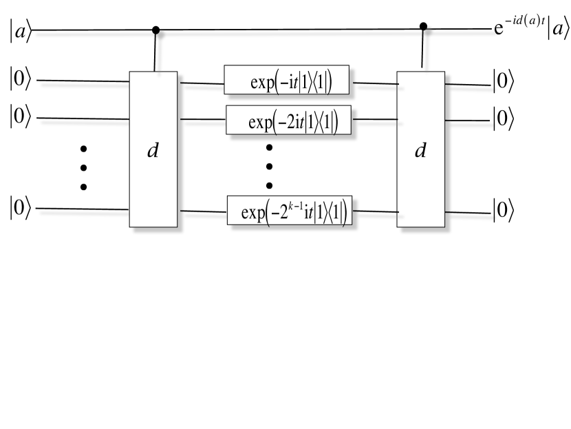
Figure 2: Simulating evolution for diagonal $\hat{H}$ with $d(a)=\langle a|\hat{H}|a\rangle\in\{0,1\}^{k}$. The row numbers $a$ of the Hamiltonian are written onto a string of qubits, and the string of qubits in the $|0\rangle$ state are ancillary. The depicted circuit circuit then effects the transformation $|a,0\rangle\mapsto|a,d(a)\rangle\mapsto{\rm e}^{-{\rm i}td(a)}|a,d(a)\rangle\mapsto{\rm e}^{-{\rm i}td(a)}|a,0\rangle={\rm e}^{-{\rm i}\hat{H}t}|a,0\rangle$.

The quantum simulation circuit is designed to approximate the desired unitary evolution operator $U$ by a sequence $\prod_{\nu=1}^{N}U_{j_{\nu}}$ where each $U_{j_{\nu}}$ is generated by one of $m$ one-sparse Hamiltonians. Generalizing the Trotter formula using the Suzuki iteration method leads to a much more efficient way of performing this unitary factorization, i.e., to a product of unitary gates with the length of this sequence of unitary gates being $t^{1+o(1)}$ [16, 17].

The Hamiltonian in the oracle is promised to be $d$-sparse with $d\in$poly$(n)$. This creates the algorithmic challenge of reducing the $d$-sparse Hamiltonian into a disjoint sum of one-sparse Hamiltonians. The decomposition is aided by first converting sparse Hamiltonians into graphs of low degree and then colouring the graph so that it is a disjoint union of degree-one graphs; hence the corresponding Hamiltonian is a direct sum of one-sparse Hamiltonians each corresponding to one colour of the graph [16, 17].

The Hamiltonian is converted to a graph as follows. Let $x$ label a row of the Hamiltonian matrix and $y$ the column. As the Hamiltonian is $d$-sparse, there are at most $d$ column numbers that hold nonzero elements for row $x$. We call these column entries $y_{1,\dots,d}$ in no particular order; i.e., the increasing sequence of indices $1,\dots,d$ does not imply increasing values of $y_{i}$. Now construct the graph by assigning each $x$ a vertex so that there are now $2^{n}$ vertices but no edges yet.

For given $x$, we construct an edge to another vertex value $x^{\prime}$ if $x^{\prime}=y_{i}$ such that $y_{i}$ is one of the column indices where row $x$ and column $y_{i}$ has a nonzero Hamiltonian matrix element. The weight of the edge is the value of that matrix element $\langle x|\hat{H}|y_{i}\rangle$. If we simplify $\hat{H}$ to having only real matrix entries and note that $\hat{H}=\hat{H}^{\dagger}$, then we can assign the Hamiltonian an undirected graph because $\langle x|\hat{H}|y_{i}\rangle=\langle y_{i}|\hat{H}|x\rangle$. The Hamiltonian is thus faithfully represented by a degree-$d$ undirected graph. A superior colouring algorithm that yields a direct sum of one-sparse Hamiltonians can reduce $T$ and $S$ costs for the associated quantum query algorithm to determine the sequence of operations for evolution generated by a $d$-sparse Hamiltonian.

Table 1 provides a summary of some advances over the years in reducing $T$ and $S$ costs. In some cases one cost is reduced at the expense of the other. Although the efficiency of quantum simulation has been known for quite some time, quantum simulations could be the first practical application of quantum computing. Cost reductions reduce the waiting time for non-trivial quantum simulations to become a reality and hence are important.

Who	Year	T	S
Lloyd[12]	1996	$O(t^{2})$	$O(n)$
AT[13]	2003	$O\left(n^{9}d^{4}\frac{t^{2}}{\epsilon}\right)$	$O(n)$
Childs[14]	2003	$O\left(n^{2}d^{4+o(1)}\frac{t^{3/2}}{\sqrt{\epsilon}}\right)$	$O\left(n\right)$
BACS[16]	2007	$O\left(\log^{*}\!nd^{4+o(1)}\frac{t^{1+1/2k}}{\epsilon^{1/2k}}\right)$	$O(n\log^{*}\!n)$
CK[18]	2010	$O\left(\left[d^{3}+d^{2}\log^{*}\!n\right]\frac{t^{1+1/2k}}{\epsilon^{1/2k}}\right)$	$O\left(nd+n\log^{*}\!n\right)$
CB[19]	2010	$O\left(\|\hat{H}\|_{\rm max}d\frac{t}{\sqrt{\epsilon}}\right)$	$\bullet$

Table 1: Key developments in reducing time $T$ and space $S$ costs for a quantum computer to simulate time-independent Hamiltonian generated evolution as a function of the number of qubits $n$ representing the system, the sparseness $d$ of the Hamiltonian, the allowed error $\epsilon$, and the norm of the Hamiltonian $\|\hat{H}\|$. The authors are listed in the first column along with references and the year in the second column. The final row and column is given by $\bullet$ to show that the space cost is not explicitly known. The iterated logarithm $\log^{*}$ in the table is the number of successive iterations of the base-two logarithm function required to reduce the number to one or less.

3 Applications

Although quantum computing was founded on the principle of quantum simulation, other algorithms such as factorization have dominated the field for many years. The reason quantum simulation is back in full force can be understood from the prescient quote from a 1997 paper by Abrams and Lloyd[6]:

But the problem of simulation — that is, the problem of modeling the full time evolution of an arbitrary quantum system — is less technologically demanding. While thousands of qubits and billions of quantum logic operations are needed to solve classical difficult factoring problems [16], it would be possible to use a quantum computer with only a few tens of qubits and a few thousand operations to perform simulations that would be classical intractable [17].

Abrams and Lloyd specifically showed that the quantum simulator would efficiently simulate fermionic systems. Combined with other results on bosonic and anionic systems, the quantum simulator is thus known to be an efficient simulator of all types of many-body systems.

Various many-body systems are considered for experimental quantum simulation in order to learn properties about the system that are unreachable with classical simulations due to intractability. Let us assign $X$, $Y$ and $Z$ as the Pauli operators on a single qubit. The Hamiltonians for these many-body systems include the Ising Hamiltonian $J\sum_{\langle i,j\rangle}Z_{i}\otimes Z_{j}+B\sum_{i}X_{i}$, the XY Hamiltonian $J_{x}\sum_{\langle i,j\rangle}X_{i}\otimes X_{j}+J_{y}\sum_{\langle i,j\rangle}Y_{i}\otimes Y_{j}$, the Heisenberg Hamiltonian $J_{x}\sum_{\langle i,j\rangle}X_{i}\otimes X_{j}+J_{y}\sum_{\langle i,j\rangle}Y_{i}\otimes Y_{j}$ and the honeycomb Hamiltonian $J_{x}\sum_{x{\rm-link}}X_{i}\otimes X_{j}-J_{y}\sum_{y{\rm-link}}Y_{i}\otimes Y_{j}-J_{z}\sum_{x{\rm-link}}Z_{i}\otimes Z_{j}$. Whereas earlier the algorithm for simulation is designed for the broadest class of simulatable Hamiltonians, if the Hamitlonian is known explicitly and is a sum of strictly local Hamiltonians, then there is a straightforward circuit-construction algorithm for unitary gates generated by a tensor product of Pauli operators [20].

Whereas quantum simulators are evidently useful for simulating quantum dynamics by design, they can be used more broadly, for example to solve giant sets of coupled linear equations [21]. This approach takes quantum simulators beyond applicability just to quantum systems, but we have to be careful about what we mean by “solve” as we had to be careful about what we meant by “solve” Schrödinger’s equation earlier.

The problem to be solved by the quantum linear equation solver can be understood by the following statement.

Given matrix $A$ vector $\bm{b}$, and matrix $M$, find a good approximation of $\bm{x}^{\rm T}M\bm{x}$ such that $A\bm{x}=\bm{b}$.

The strategy for using a quantum simulator to solve this problem is as follows. Begin by replacing $\bm{b}$ by the quantum state $|\bm{b}\rangle=\sum_{i=1}^{N}b_{i}|i\rangle$ with $|i\rangle$ the computational basis.

The solution would be $|\bm{x}\rangle=\hat{A}^{-1}|\bm{b}\rangle$, but inverting $\hat{A}$ is hard so a method has to be found to circumvent this difficulty. The operator $\hat{A}$ has eigenvalues $\lambda_{j}$ and eigenvectors $|u_{j}\rangle$ for $j=1,\ldots,N$, and we express $|\bm{b}\rangle=\sum_{j=1}^{N}\beta_{j}|u_{j}\rangle$ in the $\hat{A}$-eigenbasis. The concept is to recognize that

$$|\bm{x}\rangle=\hat{A}^{-1}|\bm{b}\rangle=\sum_{j=1}^{N}\frac{\beta_{j}}{\lambda_{j}}|u_{j}\rangle.$$ (5)

This approach is achieved by using the phase-estimation approach, namely by taking $\bm{b}\rangle$ with ancilla to obtain $\sum_{j=1}^{N}\beta_{j}|u_{j}\rangle|\lambda_{j}\rangle$. Then the non-unitary linear map $|\lambda_{j}\rangle\mapsto\lambda_{j}^{-1}|\lambda_{j}\rangle$ is constructed in a quantum circuit. Finally the circuit uncomputes $|\lambda_{j}\rangle$ to obtain the approximation $|\bm{x}\rangle$.

4 Conclusions

This article provides an overview of algorithmic quantum simulation, approaches to implementing and improving these algorithms, and applications of quantum algorithms for quantum simulation. Theoretical research in this area is challenging because it draws in so many different techniques from such different areas, for example graph theory, operator algebra, and computational complexity. The field is exciting from a technological perspective because non-trivial problems could be solved with smaller quantum computers than for other planned applications of quantum computing such as to factorization.

References

- [1] DiVincenzo, D.P.: Quantum Computation Science 270, 255–261 (1995).
- [2] Bernstein, E., Vazirani, U.: Quantum Complexity Theory. SIAM J. Comp. 26, 1411–1473 (1997).
- [3] Adcock, M.R.A., Høyer, P., Sanders, B.C.: Limitations on continuous variable quantum algorithms with Fourier transforms. New J. Phys. 11, 103035 (2009).
- [4] Buluta, I., Nori, F.: Quantum Simulators. Science 326, 108–111 (2009).
- [5] Neeley, M., Ansmann, M., Bialczak, R.C., Hofheinz, M., Lucero, E., O’Connell, A.D., Sank, D., Wang, H., Wenner, J., Cleland, A.N., Geller, M.R., Martinis, J.M.: Emulation of a Quantum Spin with a Superconducting Phase Qudit. Science 325, 722–725 (2009).
- [6] Abrams, D.S., Lloyd, S.: Simulation of Many-Body Fermi Systems on a Universal Quantum Computer. Phys. Rev. Lett. 79, 2586–2589 (1997).
- [7] Jordan, S.P., Lee, K.S.M., Preskill, J.: Quantum Algorithms for Quantum Field Theories. Science 336, 1130–1133 (2012).
- [8] Kempe, J., Kitaev, A., Regev, O.: The Complexity of the Local Hamiltonian Problem. SIAM J. Comput. 35, 1070–1097 (2006).
- [9] Wiebe, N., Berry, D.W., Høyer, P., Sanders, B.C.: Higher order decompositions of ordered operator exponentials. J. Phys. A: Math. Theor. 43, 065203 (2010).
- [10] Feynman, R.P.: Simulating physics with computers. Int. J. Theor. Phys. 21, 467–488 (1982).
- [11] Aaronson, S.: Quantum Computing since Democritus. Cambridge University Press, Cambridge UK (2013).
- [12] Lloyd, S.: Universal Quantum Simulators. Science 273, 1073–1078 (1996).
- [13] Aharonov, D., Ta-Shma, A.: Adiabatic Quantum State Generation and Statistical Zero Knowledge. In: Proc. 35th Annual ACM Symp. on Theory of Computing, New York:ACM, 20–29 (2003).
- [14] Childs, A.M.: Quantum information processing in continuous time. Ph.D. thesis, Massachusetts Institute of Technology (2004).
- [15] Childs, A.M., Cleve, R., Deotto, E., Farhi, E., Guttman, S., Spielman, D.A.: Exponential algorithmic speedup by quantum walk. In: Proc. 35th Annual ACM Symp. on Theory of Computing, New York: ACM, 59–68 (2003).
- [16] Berry, D.W., Ahokas, G., Cleve, R., and Sanders, B.C.: Efficient quantum algorithms for simulating sparse Hamiltonians. Comm. Math. Phys. 270, 359–371 (2007).
- [17] Berry, D.W., Ahokas, G., Cleve, R., and Sanders, B.C.: Quantum algorithms for Hamiltonian simulation. In: Mathematics of Quantum Computation and Quantum Technology, Chen, G., Kauffman, L., Lomonaco, S.J., eds., Ch. 4: 89–110, Taylor & Francis, Oxford (2007).
- [18] Childs, A.M., Kothari, R.: Simulating sparse Hamiltonians with star decompositions. Theory of Quantum Computation, Communication, and Cryptography (TQC 2010), LNCS 6519, 94–103 (2011).
- [19] Childs, A.M., Berry, D.W.: Black-box Hamiltonian simulation and unitary implementation. 12, 29–62 (2012).
- [20] Raeisi, S., Wiebe, N., Sanders, B.C.: Quantum-Circuit Design for Efficient Simulations of Many-Body Quantum Dynamics. New J. Phys. 14, 103017 (2012).
- [21] Harrow, A.W., Hassidim, A., Lloyd, S.: Quantum Algorithm for Linear Systems of Equations. Phys. Rev. Lett. 103, 150502 (2009).