A Brief Tutorial on Transformation Based Markov Chain Monte Carlo and Optimal Scaling of the Additive Transformation

Kushal Kr. Dey , Sourabh Bhattacharya‡+
Abstract

We consider the recently introduced Transformation-based Markov Chain Monte Carlo (TMCMC) (Dutta and Bhattacharya (2014)), a methodology that is designed to update all the parameters simultaneously using some simple deterministic transformation of a one-dimensional random variable drawn from some arbitrary distribution on a relevant support. The additive transformation based TMCMC is similar in spirit to random walk Metropolis, except the fact that unlike the latter, additive TMCMC uses a single draw from a one-dimensional proposal distribution to update the high-dimensional parameter. In this paper, we first provide a brief tutorial on TMCMC, exploring its connections and contrasts with various available MCMC methods.

Then we study the diffusion limits of additive TMCMC under various set-ups ranging from the product structure of the target density to the case where the target is absolutely continuous with respect to a Gaussian measure; we also consider the additive TMCMC within Gibbs approach for all the above set-ups. These investigations lead to appropriate scaling of the one-dimensional proposal density. We also show that the optimal acceptance rate of additive TMCMC is 0.439 under all the aforementioned set-ups, in contrast with the well-established 0.234 acceptance rate associated with optimal random walk Metropolis algorithms under the same set-ups. We also elucidate the ramifications of our results and clear advantages of additive TMCMC over random walk Metropolis with ample simulation studies and Bayesian analysis of a real, spatial dataset with which 160160160 unknowns are associated.
Keywords: Additive Transformation: Diffusion Limit; High Dimension; Optimal Scaling; Random Walk; Transformation-based Markov Chain Monte Carlo.

Department of Statistics, University of Chicago, USA

Interdisciplinary Statistical Research Unit, Indian Statistical Institute, Kolkata

++ Corresponding author: bhsourabh@gmail.com

1 Introduction

Markov Chain Monte Carlo (MCMC), particularly, the Metropolis-Hastings (MH) methods, have revolutionized Bayesian computation – this pleasing truth, however, is often hard to appreciate in the face of the challenges posed by computational complexities and convergence issues of traditional MCMC. Indeed, exploration of very high-dimensional posterior distributions using MCMC can be both computationally very expensive and troublesome convergence-wise. Thus, there seems to be trade-off between the great flexibility of MCMC algorithms (see, for example, Storvik (2011), Martino and Read (2013)) and choice of the right MCMC algorithm that ensures good convergence properties and reasonable computational complexity. Investigation of connections between varieties of available MCMC methods, as provided in the aforementioned papers, seems to be important to decide upon a suitable MCMC algorithm, given any paricular problem at hand.

The random walk Metropolis (RWM) algorithm is a popular MH algorithm because of its simplicity and ease in implementation, but unless great care is taken to properly scale the proposal distribution the algorithm can have poor convergence properties. For instance, if the variance of the proposal density is small, then the jumps will be small in magnitude, implying that the Markov chain will require a large number of iterations to explore the entire state-space. On the other hand, large variance of the proposal density causes too many rejections of the proposed moves, again considerably slowing down convergence of the underlying Markov chain. The need for an optimal choice of the proposal variance is thus inherent in the RWM algorithms. The pioneering approach towards obtaining an optimal scaling of the RWM proposal is due to Roberts et al. (1997) in the case of target densities associated with independent and identical (i.i.d.formulae-sequence𝑖𝑖𝑑i.i.d.) random variables; generalization of this work to more general set-ups are provided by Bédard (2007) (target density associated with independent but non-identical random variables) and Mattingly et al. (2011) (target density absolutely continuous with respect to a Gaussian measure). The approach used in all these works is to study the diffusion approximation of the high-dimensional RWM algorithm, and maximization of the speed of convergence of the limiting diffusion. The optimal scaling, the optimal acceptance rate and the optimal speed of convergence of the limiting diffusion, along with the complexity of the algorithm are all obtained from this powerful approach.

In practice, a serious drawback of the RWM algorithm in high dimensions is that there is always a positive probability that a particular coordinate of the high-dimensional random variable is ill-proposed; in that case the acceptance ratio will tend to be extremely small, prompting rejection of the entire high-dimensional move. In general, unless the high-dimensional proposal distribution, which need not necessarily be a random walk proposal distribution, is designed with extreme care, such problem usually persists. Unfortunately, such carefully designed proposal density is rare in high dimensions. To combat these difficulties Dutta and Bhattacharya (2014) proposed an approach where the entire block of parameters can be updated simultaneously using some simple deterministic transformation of a scalar random variable sampled from some arbitrary distribution defined on some suitable support. The strategy effectively reduces the high-dimensional proposal distribution to a one-dimensional proposal, greatly improving the acceptance rate and computational speed in the process. This methodology is no longer Metropolis-Hastings for dimensions greater than one; the proposal density in more than one dimension becomes singular because it is induced by a one-dimensional random variable. However, in one-dimensional cases this coincides with Metropolis-Hastings with a specialized mixture proposal density; in particular, the additive transformation based TMCMC coincides with RWM in one-dimensional situations. Dutta and Bhattacharya (2014) refer to this new general methodology as Transformation-based MCMC (TMCMC). In their work the authors point out several advantages of the additive transformation in comparison with the other valid transformations. For instance, they show that additive TMCMC requires less number of ‘move-types’ compared to other valid transformations; moreover, the acceptance rate has a simple form for additive transformations since the Jacobian of additive transformations is 1.

The contribution of this paper is two-fold. First, we provide a brief tutorial on TMCMC, attempting to convey the key ideas and the properties in simple terms and from several perspectives. We explore various connections and contrasts with existing MCMC algorithms.

Second, we investigate the diffusion limits of additive TMCMC in high-dimensional situations under various forms of the target density when the one-dimensional random variable used for the additive transformation is drawn from a left truncated zero-mean normal density. In particular, we consider situations when the target density corresponds to i.i.d.formulae-sequence𝑖𝑖𝑑i.i.d. random variables, independent but non-identically distributed random variables; we also study the diffusion limit of additive TMCMC when the target is absolutely continuous with respect to a Gaussian measure. Since all these forms are considered in the MCMC literature related to diffusion limits and optimal scaling of RWM, comparisons of our additive TMCMC-based approaches can be made with the respective RWM-based approaches. Furthermore, in each of the aforementioned set-ups, we also consider additive TMCMC within Gibbs approach, where one or multiple components of the high-dimensional random variable are updated by additive TMCMC, conditioning on the remaining components. This we compare with the corresponding RWM within Gibbs approach under the same settings of the target densities.

Briefly, our scaling investigations show that the optimal additive TMCMC acceptance rate in all the set-ups is 0.439, as opposed to 0.234 associated with RWM. Moreover, we point out that even though the optimal diffusion speed of RWM is slightly greater than that of additive TMCMC, the diffusion speed associated with additive TMCMC is more robust with respect to the choice of the scaling constant. In other words, if the optimal scaling constant for RWM is somewhat altered, this triggers a sharp fall in the diffusion speed, but in the case of additive TMCMC the rate of decrease of diffusion speed is much slower. Investigation of the consequences of this phenomenon with simulation studies reveal severe decline in the performance of RWM in comparison with additive TMCMC.

This non-robustness of RWM with respect to scale choices other than the optimal, presents quite important consequences for applied MCMC practitioners, which we elaborate with a real, spatial data analysis problem. In a nutshell, in the context of the spatial problem, we have provided a method, which appears to be generally applicable, for approximately achieving 44% and 23% acceptance rates for additive TMCMC and RWM; however, achieving the desired acceptance rates in general problems where optimal scaling theories are yet lacking, does not guarantee that the achieved acceptance rates correspond to optimal scales, as there are usually very many scale choices corresponding to the same acceptance rate. Because of such sub-optimality, in the real spatial problem, RWM faces very serious performance problems. On the other hand, additive TMCMC, because of its robustness with respect to the scales, performs quite reasonably.

Our paper is structured as follows. In Section 2, we provide a brief tutorial on TMCMC. We develop the theory for optimal additive TMCMC scaling in the i.i.d.formulae-sequence𝑖𝑖𝑑i.i.d. set-up in Section 3; in the same section (Section 3.1) we also develop the corresponding theory for additive TMCMC within Gibbs in the i.i.d.formulae-sequence𝑖𝑖𝑑i.i.d. situation. In Section 4, we extend the additive TMCMC-based optimal scaling theory to the independent but non-identical set-up; in Section 4.1 we outline the corresponding TMCMC within Gibbs case. We then further extend our additive TMCMC based optimal scaling theory to the aforementioned dependent set-up in Section 5, presenting the formal result in Section 5.2; the corresponding TMCMC within Gibbs case is considered in Section 5.3. In Section 6, we provide numerical comparisons between additive TMCMC and RWM in terms of optimal acceptance rates and diffusion speeds; in Section 7, we illustrate our theoretical results and compare the performances of additive TMCMC and RWM using simulation studies, illustrating that the former is a far more effective algorithm in comparison with the latter. In Section 8, we compare additive TMCMC with RWM with respect to a 160160160-dimensional posterior density associated with a real, spatial dataset, vividly demonstrating the clear superiority of additive TMCMC over RWM. Finally, we make concluding remarks in Section 9.

Apart from the main developments provided in this article, we provide additional details in our supplementary material Dey and Bhattacharya (2016c), whose sections and figures have the prefix “S-” when referred to in this article. Briefly, in Section S-1, we provide details on computational efficiency of TMCMC. Specifically, we demonstrate with an experiment the superior computational speed of additive TMCMC in comparison with RWM, particularly in high dimensions. In Section S-2 we discuss, with appropriate experiments, the necessity of optimal scaling in additive TMCMC, while in Sections S-3 and S-4 we delve into the robustness issues associated with the scale choices of additive TMCMC and RWM. In Section S-5, we include brief discussions of adaptive versions of RWM and TMCMC. Moreover, the proofs of all our technical results are provided in Sections S-6 and S-7 of the supplement.

2 A brief overview of TMCMC

Suppose that we are simulating from a d𝑑d dimensional space (usually dsuperscript𝑑\mathbb{R}^{d}, where \mathbb{R} is the real line), and suppose we are currently at a point x=(x1,,xd)𝑥subscript𝑥1subscript𝑥𝑑x=(x_{1},\ldots,x_{d}). Let us define the d𝑑d-dimensional random vector b=(b1,,bd)𝑏subscript𝑏1subscript𝑏𝑑b=(b_{1},\ldots,b_{d}), such that, for i=1,,d𝑖1𝑑i=1,\ldots,d,

bi={+1with probabilitypi;0with probability1piqi;1with probabilityqi,subscript𝑏𝑖cases1with probabilitysubscript𝑝𝑖0with probability1subscript𝑝𝑖subscript𝑞𝑖1with probabilitysubscript𝑞𝑖b_{i}=\left\{\begin{array}[]{ccc}+1&\mbox{with probability}&p_{i};\\ 0&\mbox{with probability}&1-p_{i}-q_{i};\\ -1&\mbox{with probability}&q_{i},\end{array}\right. (1)

where, for each i𝑖i, 0<pi,qi<1formulae-sequence0subscript𝑝𝑖subscript𝑞𝑖10<p_{i},q_{i}<1 such that pi+qi1subscript𝑝𝑖subscript𝑞𝑖1p_{i}+q_{i}\leq 1. Let ϵϱ(ϵ)=ϱ~(ϵ)I𝕊(ϵ)similar-toitalic-ϵitalic-ϱitalic-ϵ~italic-ϱitalic-ϵsubscript𝐼𝕊italic-ϵ\epsilon\sim\varrho(\epsilon)=\tilde{\varrho}(\epsilon)I_{\mathbb{S}}(\epsilon), where ϱ~()~italic-ϱ\tilde{\varrho}(\cdot) is any arbitrary density supported on some suitable space 𝕊𝕊\mathbb{S}; here I𝕊()subscript𝐼𝕊I_{\mathbb{S}}(\cdot) denotes the indicator function of 𝕊𝕊\mathbb{S}.

TMCMC uses moves of the following type:

(x1,,xd)(Tb1(x1,ϵ),,Tbd(xd,ϵ)),subscript𝑥1subscript𝑥𝑑superscript𝑇subscript𝑏1subscript𝑥1italic-ϵsuperscript𝑇subscript𝑏𝑑subscript𝑥𝑑italic-ϵ(x_{1},\ldots,x_{d})\rightarrow(T^{b_{1}}(x_{1},\epsilon),\ldots,T^{b_{d}}(x_{d},\epsilon)), (2)

where T+1(xi,ϵ)superscript𝑇1subscript𝑥𝑖italic-ϵT^{+1}(x_{i},\epsilon), the forward transformation to coordinate xisubscript𝑥𝑖x_{i}, and T1(xi,ϵ)superscript𝑇1subscript𝑥𝑖italic-ϵT^{-1}(x_{i},\epsilon), the backward transformation to xisubscript𝑥𝑖x_{i}, are bijective for fixed ϵitalic-ϵ\epsilon and injective for fixed xisubscript𝑥𝑖x_{i}, satisfying

T+1(T1(xi,ϵ),ϵ)=T1(T+1(xi,ϵ),ϵ)=xi.superscript𝑇1superscript𝑇1subscript𝑥𝑖italic-ϵitalic-ϵsuperscript𝑇1superscript𝑇1subscript𝑥𝑖italic-ϵitalic-ϵsubscript𝑥𝑖T^{+1}(T^{-1}(x_{i},\epsilon),\epsilon)=T^{-1}(T^{+1}(x_{i},\epsilon),\epsilon)=x_{i}. (3)

The transformation

T0(xi,ϵ)xi,ϵ𝕊,formulae-sequencesuperscript𝑇0subscript𝑥𝑖italic-ϵsubscript𝑥𝑖for-allitalic-ϵ𝕊T^{0}(x_{i},\epsilon)\equiv x_{i},~{}\forall\epsilon\in\mathbb{S}, (4)

indicates no change to the coordinate xisubscript𝑥𝑖x_{i} while updating the vector x=(x1,,xd)𝑥subscript𝑥1subscript𝑥𝑑x=(x_{1},\ldots,x_{d}) to x=𝒯b(x,ϵ)superscript𝑥subscript𝒯𝑏𝑥italic-ϵx^{*}=\mathcal{T}_{b}(x,\epsilon), where 𝒯b(x,ϵ)subscript𝒯𝑏𝑥italic-ϵ\mathcal{T}_{b}(x,\epsilon) denotes the updated vector (Tb1(x1,ϵ),,Tbd(xd,ϵ))superscript𝑇subscript𝑏1subscript𝑥1italic-ϵsuperscript𝑇subscript𝑏𝑑subscript𝑥𝑑italic-ϵ(T^{b_{1}}(x_{1},\epsilon),\ldots,T^{b_{d}}(x_{d},\epsilon)). Assuming for simplicity of illustration that pi=qisubscript𝑝𝑖subscript𝑞𝑖p_{i}=q_{i} for i=1,,d𝑖1𝑑i=1,\ldots,d, move (2) is to be accepted with probability

α=min{1,π(x)π(x)Jb(x,ϵ)},𝛼1𝜋superscript𝑥𝜋𝑥superscript𝐽𝑏𝑥italic-ϵ\alpha=\min\left\{1,\frac{\pi(x^{*})}{\pi(x)}J^{b}(x,\epsilon)\right\}, (5)

where Jb(x,ϵ)=|(𝒯b(x,ϵ),ϵ)(x,ϵ)|superscript𝐽𝑏𝑥italic-ϵsuperscript𝒯𝑏𝑥italic-ϵitalic-ϵ𝑥italic-ϵJ^{b}(x,\epsilon)=\left|\frac{\partial(\mathcal{T}^{b}(x,\epsilon),\epsilon)}{\partial(x,\epsilon)}\right| is the Jacobian of the transformation associated with 𝒯bsuperscript𝒯𝑏\mathcal{T}^{b}. For general (p1,,pd)subscript𝑝1subscript𝑝𝑑(p_{1},\ldots,p_{d}) and (q1,,qd)subscript𝑞1subscript𝑞𝑑(q_{1},\ldots,q_{d}), the acceptance ratio depends upon these probabilities; see Dutta and Bhattacharya (2014).

2.1 Detailed balance

In the supplement to Dutta and Bhattacharya (2014) the proof of detailed balance has been provided, but here we refurnish the proof with more details and with more intuitive discussion. For the purpose of detailed balance, we need the following definition of “conjugate” bc=(b1c,,bdc)superscript𝑏𝑐subscriptsuperscript𝑏𝑐1subscriptsuperscript𝑏𝑐𝑑b^{c}=(b^{c}_{1},\ldots,b^{c}_{d}) of the random vector d𝑑d:

bic={+1with probabilityqi;0with probability1piqi;1with probabilitypi,subscriptsuperscript𝑏𝑐𝑖cases1with probabilitysubscript𝑞𝑖0with probability1subscript𝑝𝑖subscript𝑞𝑖1with probabilitysubscript𝑝𝑖b^{c}_{i}=\left\{\begin{array}[]{ccc}+1&\mbox{with probability}&q_{i};\\ 0&\mbox{with probability}&1-p_{i}-q_{i};\\ -1&\mbox{with probability}&p_{i},\end{array}\right. (6)

This definition is needed for returning to x𝑥x from xsuperscript𝑥x^{*}, so that moving from x𝑥x to xsuperscript𝑥x^{*} using the transformation 𝒯bsuperscript𝒯𝑏\mathcal{T}^{b} has, in essence, the same probability as returning from xsuperscript𝑥x^{*} to x𝑥x using the transformation 𝒯bcsuperscript𝒯superscript𝑏𝑐\mathcal{T}^{b^{c}}. Details are provided below; at this point we note that for the i𝑖i-th coordinate xisubscript𝑥𝑖x_{i}, the probability of making a forward move to xisubscriptsuperscript𝑥𝑖x^{*}_{i} using T+1(xi,ϵ)superscript𝑇1subscript𝑥𝑖italic-ϵT^{+1}(x_{i},\epsilon) is pisubscript𝑝𝑖p_{i}, which is also the probability of returning from xisubscriptsuperscript𝑥𝑖x^{*}_{i} to xisubscript𝑥𝑖x_{i} using the backward move T1(xi,ϵ)=T(+1)c(xi,ϵ)superscript𝑇1subscriptsuperscript𝑥𝑖italic-ϵsuperscript𝑇superscript1𝑐subscriptsuperscript𝑥𝑖italic-ϵT^{-1}(x^{*}_{i},\epsilon)=T^{(+1)^{c}}(x^{*}_{i},\epsilon).

Letting K𝐾K denote the Markov transition kernel associated with TMCMC, note that for moving from x𝑥x to xsuperscript𝑥x^{*}, the kernel satisfies

π(x)K(xx)𝜋𝑥𝐾𝑥superscript𝑥\displaystyle\pi(x)K(x\rightarrow x^{*}) =π(x)P(b)ϱ(ϵ)min{1,π(x)π(x)Jb(x,ϵ)}absent𝜋𝑥𝑃𝑏italic-ϱitalic-ϵ1𝜋superscript𝑥𝜋𝑥superscript𝐽𝑏𝑥italic-ϵ\displaystyle=\pi(x)P(b)\varrho(\epsilon)\min\left\{1,\frac{\pi(x^{*})}{\pi(x)}J^{b}(x,\epsilon)\right\}
=min{π(x)P(b)ϱ(ϵ),P(b)ϱ(ϵ)π(x)Jb(x,ϵ)},absent𝜋𝑥𝑃𝑏italic-ϱitalic-ϵ𝑃𝑏italic-ϱitalic-ϵ𝜋superscript𝑥superscript𝐽𝑏𝑥italic-ϵ\displaystyle=\min\left\{\pi(x)P(b)\varrho(\epsilon),P(b)\varrho(\epsilon)\pi(x^{*})J^{b}(x,\epsilon)\right\}, (7)

where P(b)𝑃𝑏P(b) is the probability of b𝑏b responsible for the movement of the underlying Markov chain from x𝑥x to xsuperscript𝑥x^{*}. For returning from xsuperscript𝑥x^{*} to x𝑥x, the kernel satisfies

π(x)K(xx)𝜋superscript𝑥𝐾superscript𝑥𝑥\displaystyle\pi(x^{*})K(x^{*}\rightarrow x) =π(x)P(bc)ϱ(ϵ)Jb(x,ϵ)min{1,π(x)π(x)Jbc(x,ϵ)}absent𝜋superscript𝑥𝑃superscript𝑏𝑐italic-ϱitalic-ϵsuperscript𝐽𝑏𝑥italic-ϵ1𝜋𝑥𝜋superscript𝑥superscript𝐽superscript𝑏𝑐superscript𝑥italic-ϵ\displaystyle=\pi(x^{*})P(b^{c})\varrho(\epsilon)J^{b}(x,\epsilon)\min\left\{1,\frac{\pi(x)}{\pi(x^{*})}J^{b^{c}}(x^{*},\epsilon)\right\}
=min{π(x)P(bc)ϱ(ϵ)Jb(x,ϵ),π(x)P(bc)ϱ(ϵ)Jb(x,ϵ)×Jbc(x,ϵ)},absent𝜋superscript𝑥𝑃superscript𝑏𝑐italic-ϱitalic-ϵsuperscript𝐽𝑏𝑥italic-ϵ𝜋𝑥𝑃superscript𝑏𝑐italic-ϱitalic-ϵsuperscript𝐽𝑏𝑥italic-ϵsuperscript𝐽superscript𝑏𝑐superscript𝑥italic-ϵ\displaystyle=\min\left\{\pi(x^{*})P(b^{c})\varrho(\epsilon)J^{b}(x,\epsilon),\pi(x)P(b^{c})\varrho(\epsilon)J^{b}(x,\epsilon)\times J^{b^{c}}(x^{*},\epsilon)\right\},
=min{π(x)P(bc)ϱ(ϵ)Jb(x,ϵ),π(x)P(bc)ϱ(ϵ)Jb(x,ϵ)×Jbc(x,ϵ)}.absent𝜋superscript𝑥𝑃superscript𝑏𝑐italic-ϱitalic-ϵsuperscript𝐽𝑏𝑥italic-ϵ𝜋𝑥𝑃superscript𝑏𝑐italic-ϱitalic-ϵsuperscript𝐽𝑏𝑥italic-ϵsuperscript𝐽superscript𝑏𝑐superscript𝑥italic-ϵ\displaystyle=\min\left\{\pi(x^{*})P(b^{c})\varrho(\epsilon)J^{b}(x,\epsilon),\pi(x)P(b^{c})\varrho(\epsilon)J^{b}(x,\epsilon)\times J^{b^{c}}(x^{*},\epsilon)\right\}.

It follows from (3) and (4) that 𝒯bc(𝒯b(x,ϵ))=xsuperscript𝒯superscript𝑏𝑐superscript𝒯𝑏𝑥italic-ϵ𝑥\mathcal{T}^{b^{c}}(\mathcal{T}^{b}(x,\epsilon))=x, so that

Jb(x,ϵ)×Jbc(x,ϵ)superscript𝐽𝑏𝑥italic-ϵsuperscript𝐽superscript𝑏𝑐superscript𝑥italic-ϵ\displaystyle J^{b}(x,\epsilon)\times J^{b^{c}}(x^{*},\epsilon)
=|(𝒯b(x,ϵ),ϵ)(x,ϵ)|×|(𝒯bc(𝒯b(x,ϵ)),ϵ)(𝒯b(x,ϵ),ϵ)|absentsuperscript𝒯𝑏𝑥italic-ϵitalic-ϵ𝑥italic-ϵsuperscript𝒯superscript𝑏𝑐superscript𝒯𝑏𝑥italic-ϵitalic-ϵsuperscript𝒯𝑏𝑥italic-ϵitalic-ϵ\displaystyle=\left|\frac{\partial(\mathcal{T}^{b}(x,\epsilon),\epsilon)}{\partial(x,\epsilon)}\right|\times\left|\frac{\partial(\mathcal{T}^{b^{c}}(\mathcal{T}^{b}(x,\epsilon)),\epsilon)}{\partial(\mathcal{T}^{b}(x,\epsilon),\epsilon)}\right|
=|(𝒯b(x,ϵ),ϵ)(x,ϵ)|×|(x,ϵ)(𝒯b(x,ϵ),ϵ)|absentsuperscript𝒯𝑏𝑥italic-ϵitalic-ϵ𝑥italic-ϵ𝑥italic-ϵsuperscript𝒯𝑏𝑥italic-ϵitalic-ϵ\displaystyle=\left|\frac{\partial(\mathcal{T}^{b}(x,\epsilon),\epsilon)}{\partial(x,\epsilon)}\right|\times\left|\frac{\partial(x,\epsilon)}{\partial(\mathcal{T}^{b}(x,\epsilon),\epsilon)}\right|
=1.absent1\displaystyle=1. (9)

Substituting (9) in (LABEL:eq:detailed_balance2) we obtain

π(x)K(xx)=min{π(x)P(bc)g(ϵ)Jb(x,ϵ),π(x)P(bc)g(ϵ)}.𝜋superscript𝑥𝐾superscript𝑥𝑥𝜋superscript𝑥𝑃superscript𝑏𝑐𝑔italic-ϵsuperscript𝐽𝑏𝑥italic-ϵ𝜋𝑥𝑃superscript𝑏𝑐𝑔italic-ϵ\pi(x^{*})K(x^{*}\rightarrow x)=\min\left\{\pi(x^{*})P(b^{c})g(\epsilon)J^{b}(x,\epsilon),\pi(x)P(b^{c})g(\epsilon)\right\}. (10)

If, for simplicity of illustration we assume pi=qisubscript𝑝𝑖subscript𝑞𝑖p_{i}=q_{i} for i=1,,d𝑖1𝑑i=1,\ldots,d, it follows that P(b)=P(bc)𝑃𝑏𝑃superscript𝑏𝑐P(b)=P(b^{c}), so that (10) is equal to (7), proving detailed balance. Detailed balance of course holds for general probabilities (p1,,pd)subscript𝑝1subscript𝑝𝑑(p_{1},\ldots,p_{d}) and (q1,,qd)subscript𝑞1subscript𝑞𝑑(q_{1},\ldots,q_{d}); see the supplement of Dutta and Bhattacharya (2014).

2.2 Discussion on the independence of the acceptance probability of the proposal density ϱitalic-ϱ\varrho

An important feature of the TMCMC acceptance probability distinguishing it from the acceptance probability of the Metropolis-Hastings algorithms is its independence of the proposal density ϱitalic-ϱ\varrho, irrespective of whether or not it is symmetric, and for all valid transformations Tbsuperscript𝑇𝑏T^{b}. The reason for this is implicit in the above detailed balance arguments – the same ϵitalic-ϵ\epsilon is generated from the proposal density ϱitalic-ϱ\varrho while moving forward from x𝑥x to xsuperscript𝑥x^{*} as well as while returning to x𝑥x from xsuperscript𝑥x^{*}. This is exactly the reason why ϱ(ϵ)italic-ϱitalic-ϵ\varrho(\epsilon) features in both (7) and (LABEL:eq:detailed_balance2). Consequently, detailed balance is satisfied only if the acceptance ratio of TMCMC is independent of ϱitalic-ϱ\varrho.

2.3 Relationship of TMCMC with the MH methodology

Note that, although in Section 2 we indicated a single random variable ϵitalic-ϵ\epsilon to be used in the transformations, it is permissible to use k𝑘k random variables {ϵ1,,ϵk}subscriptitalic-ϵ1subscriptitalic-ϵ𝑘\left\{\epsilon_{1},\ldots,\epsilon_{k}\right\}, where k{1,,d}𝑘1𝑑k\in\left\{1,\ldots,d\right\}. Here it is also important to remark that general TMCMC with k=d𝑘𝑑k=d does not reduce to general MH method for the very reason that the acceptance ratio of TMCMC is always independent of the proposal density, while in MH it is not. For dimension d=1𝑑1d=1, however, TMCMC boils down to an MH algorithm with a specialized two-component mixture proposal density, where the mixture components correspond to the two available move types, forward and backward. See Dutta and Bhattacharya (2014) for the complete technical details.

As pointed out by a reviewer, TMCMC can be viewed as a MH within Gibbs methodology, which updates the variables one at a time using general MH (Geyer (2011) criticizes this terminology since Gibbs is a special case of MH). This can be seen as follows. Suppose that we assign positive probabilities to the sets b~i=(b1=0,,bi1=0,bi,bi+1=0,,bd=0)subscript~𝑏𝑖formulae-sequencesubscript𝑏10formulae-sequencesubscript𝑏𝑖10subscript𝑏𝑖formulae-sequencesubscript𝑏𝑖10subscript𝑏𝑑0\tilde{b}_{i}=(b_{1}=0,\ldots,b_{i-1}=0,b_{i},b_{i+1}=0,\ldots,b_{d}=0), for i=1,,d𝑖1𝑑i=1,\ldots,d, where bi{1,0,1}subscript𝑏𝑖101b_{i}\in\{-1,0,1\}. For TMCMC, at each iteration, we can select one of the sets b~isubscript~𝑏superscript𝑖\tilde{b}_{i^{*}} by choosing i{1,,d}superscript𝑖1𝑑i^{*}\in\{1,\ldots,d\} at random, and generate bi{1,0,1}subscript𝑏superscript𝑖101b_{i^{*}}\in\{-1,0,1\} with probabilities qisubscript𝑞superscript𝑖q_{i^{*}}, 1piqi1subscript𝑝superscript𝑖subscript𝑞superscript𝑖1-p_{i^{*}}-q_{i^{*}} and pisubscript𝑝superscript𝑖p_{i^{*}}. The corresponding xisubscript𝑥superscript𝑖x_{i^{*}}, corresponding to bisubscript𝑏superscript𝑖b_{i^{*}}, is then updated according to the TMCMC mechanism. This being a single-dimensional TMCMC step, coincides with an MH within Gibbs procedure with a specialized proposal mechanism.

2.4 Additive and multiplicative transformations in TMCMC

2.4.1 Additive TMCMC

The additive TMCMC, which is of our interest in this work, uses moves of the following type:

(x1,,xd)(x1+b1ϵ,,xd+bdϵ),subscript𝑥1subscript𝑥𝑑subscript𝑥1subscript𝑏1italic-ϵsubscript𝑥𝑑subscript𝑏𝑑italic-ϵ(x_{1},\ldots,x_{d})\rightarrow(x_{1}+b_{1}\epsilon,\ldots,x_{d}+b_{d}\epsilon),

where ϵϱ(ϵ)similar-toitalic-ϵitalic-ϱitalic-ϵ\epsilon\sim\varrho(\epsilon). Here ϱ()italic-ϱ\varrho(\cdot) is an arbitrary density with support +subscript\mathbb{R}_{+}, the positive part of the real line. In other words, we assume that Tbi(xi,ϵ)=xi+biϵsuperscript𝑇subscript𝑏𝑖subscript𝑥𝑖italic-ϵsubscript𝑥𝑖subscript𝑏𝑖italic-ϵT^{b_{i}}(x_{i},\epsilon)=x_{i}+b_{i}\epsilon. In this work, we shall assume that pi=1/2subscript𝑝𝑖12p_{i}=1/2 and qi=1/2subscript𝑞𝑖12q_{i}=1/2 for i=1,,d𝑖1𝑑i=1,\ldots,d, so that the probabilities of choosing bi=0subscript𝑏𝑖0b_{i}=0 and bic=0subscriptsuperscript𝑏𝑐𝑖0b^{c}_{i}=0 are zero. Indeed, as proved in Dutta and Bhattacharya (2014), this is a completely valid and efficient choice for additive transformations. For this work we set ϱ(ϵ)I{ϵ>0}N(0,2d)I{ϵ>0}italic-ϱitalic-ϵsubscript𝐼italic-ϵ0𝑁0superscript2𝑑subscript𝐼italic-ϵ0\varrho(\epsilon)I_{\{\epsilon>0\}}\equiv N(0,\frac{\ell^{2}}{d})I_{\{\epsilon>0\}}.

Note that, for each i𝑖i, biϵN(0,2d)similar-tosubscript𝑏𝑖italic-ϵ𝑁0superscript2𝑑b_{i}\epsilon\sim N(0,\frac{\ell^{2}}{d}), but even though biϵsubscript𝑏𝑖italic-ϵb_{i}\epsilon are pairwise uncorrelated (E(biϵ×bjϵ)=0𝐸subscript𝑏𝑖italic-ϵsubscript𝑏𝑗italic-ϵ0E(b_{i}\epsilon\times b_{j}\epsilon)=0 for ij𝑖𝑗i\neq j), they are not independent since all of them involve the same ϵitalic-ϵ\epsilon. Also observe that biϵ+bjϵ=0subscript𝑏𝑖italic-ϵsubscript𝑏𝑗italic-ϵ0b_{i}\epsilon+b_{j}\epsilon=0 with probability 1/2121/2 for ij𝑖𝑗i\neq j, showing that the linear combinations of biϵsubscript𝑏𝑖italic-ϵb_{i}\epsilon need not be normal. In other words, the joint distribution of (b1ϵ,,bdϵ)subscript𝑏1italic-ϵsubscript𝑏𝑑italic-ϵ(b_{1}\epsilon,\ldots,b_{d}\epsilon) is not normal, even though the marginal distributions are normal and the components are pairwise uncorrelated. This also shows that biϵsubscript𝑏𝑖italic-ϵb_{i}\epsilon are not independent, because independence would imply joint normality of the components.

Thus, a single ϵitalic-ϵ\epsilon is simulated from a truncated normal distribution, which is then either added to, or subtracted from each of the d𝑑d coordinates of x𝑥x with probability 1/2121/2. Assuming that the target distribution is proportional to π𝜋\pi, the new move x=(x1+b1ϵ,,xd+bdϵ)superscript𝑥subscript𝑥1subscript𝑏1italic-ϵsubscript𝑥𝑑subscript𝑏𝑑italic-ϵx^{*}=(x_{1}+b_{1}\epsilon,\ldots,x_{d}+b_{d}\epsilon) is accepted with probability

α=min{1,π(x)π(x)}.𝛼1𝜋superscript𝑥𝜋𝑥\alpha=\min\left\{1,\frac{\pi(x^{*})}{\pi(x)}\right\}. (11)

The RWM algorithm, unlike additive TMCMC, proceeds by simulating ϵ1,,ϵdsubscriptitalic-ϵ1subscriptitalic-ϵ𝑑\epsilon_{1},\ldots,\epsilon_{d} independently from N(0,2d)𝑁0superscript2𝑑N(0,\frac{\ell^{2}}{d}), and then adding ϵisubscriptitalic-ϵ𝑖\epsilon_{i} to the coordinate xisubscript𝑥𝑖x_{i}, for each i𝑖i. The new move is accepted with probability having the same form as (11). As discussed in Section 2.3 for TMCMC it is permissible to use k𝑘k random variables {ϵ1,,ϵk}subscriptitalic-ϵ1subscriptitalic-ϵ𝑘\left\{\epsilon_{1},\ldots,\epsilon_{k}\right\}, where k{1,,d}𝑘1𝑑k\in\left\{1,\ldots,d\right\}. Thus, with such a proposal, if k=d𝑘𝑑k=d, additive TMCMC reduces to RWM, showing that the latter is a special case of the former.

Discussion of computational efficiency of TMCMC is already provided in Dutta and Bhattacharya (2014). In this article, we supplement the discussion by demonstrating with an experiment the substantial computational gains of additive TMCMC over RWM, particularly in high dimensions; see Section S-1.

2.4.2 Multiplicative TMCMC

In contrast with additive TMCMC, multiplicative TMCMC proceeds by generating ϵitalic-ϵ\epsilon from some relevant distribution ϱ(ϵ)italic-ϱitalic-ϵ\varrho(\epsilon) supported on [1,1]\{0}\110[-1,1]\backslash\{0\} and then either multiplying or dividing the current states by ϵitalic-ϵ\epsilon. In this case, it is necessary to assign positive probabilities to bi=0subscript𝑏𝑖0b_{i}=0 and bic=0subscriptsuperscript𝑏𝑐𝑖0b^{c}_{i}=0 to ensure irreducibility. For i=1,,d𝑖1𝑑i=1,\ldots,d, the general multiplicative TMCMC algorithm applies the transformation xiϵbisubscript𝑥𝑖superscriptitalic-ϵsubscript𝑏𝑖x_{i}\epsilon^{b_{i}} to xisubscript𝑥𝑖x_{i}, which necessitates multiplication of the Jacobian ϵi=1dbisuperscriptitalic-ϵsuperscriptsubscript𝑖1𝑑subscript𝑏𝑖\epsilon^{\sum_{i=1}^{d}b_{i}} to the ratio of the target distribution evaluated at the new and current states, for computation of the acceptance ratio; see Dutta (2012), Dutta and Bhattacharya (2014) and Dey and Bhattacharya (2016b).

There is an alternative version of multiplicative TMCMC that proceeds by generating ϵitalic-ϵ\epsilon from ϱ(ϵ)italic-ϱitalic-ϵ\varrho(\epsilon) that is supported on (0,1]01(0,1], then making the transformation xicixiϵbimaps-tosubscript𝑥𝑖subscript𝑐𝑖subscript𝑥𝑖superscriptitalic-ϵsubscript𝑏𝑖x_{i}\mapsto c_{i}x_{i}\epsilon^{b_{i}}, where ci=1subscript𝑐𝑖1c_{i}=1 with probability risubscript𝑟𝑖r_{i} and 11-1 with probability 1ri1subscript𝑟𝑖1-r_{i}, where 0<ri<10subscript𝑟𝑖10<r_{i}<1. Here, it is again permissible to set the probabilities of bi=0subscript𝑏𝑖0b_{i}=0 and bic=0subscriptsuperscript𝑏𝑐𝑖0b^{c}_{i}=0 to zero. The Jacobian remains the same as in the previous multiplicative version.

Note that the multiplicative proposal allows relatively large jumps, while the additive moves are local in nature. Hence, judicious combination of the two proposals may allow local moves as well as large jumps, which would result in a more efficient algorithm compared to the individual proposals. Indeed, Dey and Bhattacharya (2016b) demonstrate that a mixture of the additive and multiplicative transformations outperforms individual additive TMCMC and multiplicative TMCMC.

2.4.3 Additive-multiplicative TMCMC

Apart from these TMCMC mechanisms where all the coordinates are given either additive transformation or multiplicative transformation, it is possible to give additive transformation to some coordinates and multiplicative to the rest; this TMCMC mechanism has been referred to as additive-multiplicative TMCMC in Dutta and Bhattacharya (2014) and Dey and Bhattacharya (2016b).

2.5 A manifold interpretation of the TMCMC proposal mechanism

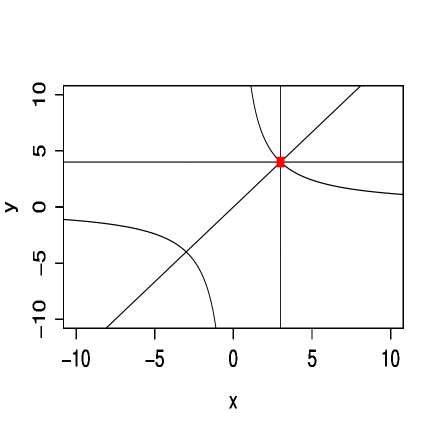
A reviewer observed that for a d𝑑d-dimensional target distribution, the TMCMC proposal can be viewed as generating points in a manifold 𝕄𝕄\mathbb{M} such that 𝕄d𝕄superscript𝑑\mathbb{M}\subseteq\mathbb{R}^{d}. For instance, for additive TMCMC this manifold 𝕄𝕄\mathbb{M} is formed by hyperplanes within dsuperscript𝑑\mathbb{R}^{d}.

Refer to caption
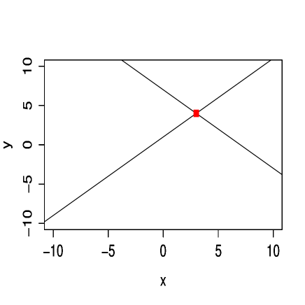
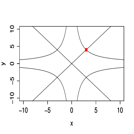
Figure 1: Relevant manifold representing the one-step proposal mechanism for additive TMCMC for d=2𝑑2d=2 given the current state, denoted by the red patch.

When d=2𝑑2d=2, Figure 1 depicts the manifold as intersecting straight lines with the current state (x1,x2)subscript𝑥1subscript𝑥2(x_{1},x_{2}) being the point of intersection. For the two versions of multiplicative TMCMC, the manifolds are shown in Figures 2 and 3 respectively.
Refer to caption
Figure 2: Relevant manifold representing the one-step proposal mechanism for the first version of multiplicative TMCMC for d=2𝑑2d=2 given the current state, denoted by the red patch.
Refer to caption
Figure 3: Relevant manifold representing the one-step proposal mechanism for the second version of multiplicative TMCMC for d=2𝑑2d=2 given the current state, denoted by the red patch.

The TMCMC proposal implicitly describes the manifold parametrically, where ϵkitalic-ϵsuperscript𝑘\epsilon\in\mathbb{R}^{k} plays the role of the parameter. If k=1𝑘1k=1, the proposed values must belong to appropriate curves embedded in dsuperscript𝑑\mathbb{R}^{d}. It is important to clarify, as the reviewer also observed, that ϱ(ϵ)italic-ϱitalic-ϵ\varrho(\epsilon) does not completely define the TMCMC proposal; the complete TMCMC proposal consists of first generating ϵitalic-ϵ\epsilon from ϱitalic-ϱ\varrho and then transforming the current state deterministically with the help of ϵitalic-ϵ\epsilon in a way that ensures the transformed state falls within the appropriate manifold.

Since, for d>1𝑑1d>1, 𝕄d𝕄superscript𝑑\mathbb{M}\subset\mathbb{R}^{d} even for k=d𝑘𝑑k=d, the above manifold viewpoint also succeeds in explaining why, even for k=d𝑘𝑑k=d, the TMCMC proposal does not reduce, in general, to the standard MH methodology. This perspective also clearly shows the singularity of the proposal, which also explains the association of the Jacobian with the acceptance probability of TMCMC. Note that for d=1𝑑1d=1 (so that k=1𝑘1k=1), however, we must have 𝕄=𝕄\mathbb{M}=\mathbb{R}.

2.6 Contrast of TMCMC with deterministic transformation based generalized Gibbs/MH approaches

TMCMC uses deterministic transformations to update the variables; however, deterministic transformations have also been considered by Liu and Yu (1999), Liu and Sabatti (2000), Kou et al. (2005) in an attempt to improve mixing behaviour of the underlying usual Gibbs or MH algorithm. In a nutshell, these authors apply suitable deterministic transformations, usually additive, as (x1,,xd)(x1+ϵ,,xd+ϵ)subscript𝑥1subscript𝑥𝑑subscript𝑥1italic-ϵsubscript𝑥𝑑italic-ϵ(x_{1},\ldots,x_{d})\rightarrow(x_{1}+\epsilon,\ldots,x_{d}+\epsilon), or multiplicative, (x1,,xd)(ηx1,,ηxd)subscript𝑥1subscript𝑥𝑑𝜂subscript𝑥1𝜂subscript𝑥𝑑(x_{1},\ldots,x_{d})\rightarrow(\eta x_{1},\ldots,\eta x_{d}), to the samples generated at each iteration of Gibbs or MH in a way that the stationarity of the target distribution is preserved, while mixing properties of chain after the transformation may perhaps be improved. To maintain stationarity, ϵitalic-ϵ\epsilon and η𝜂\eta must be simulated from some appropriate distribution which is often impossible to generate from (see Liu and Yu (1999)). To alleviate the problem Liu and Sabatti (2000) (see also Kou et al. (2005)) suggest MH methods.

As pointed out in the supplement of Dutta and Bhattacharya (2014), these generalized Gibbs/MH methods are mere attempts towards improving mixing of the underlying MCMC. These are not stand-alone methodologies which can converge to the target by themselves, unlike TMCMC. In fact, as shown in the supplement of Dutta and Bhattacharya (2014) the aforementioned additive and multiplicative transformations of generalized Gibbs/MH approaches are themselves not even irreducible, and are hence generally non-convergent. See the supplement of Dutta and Bhattacharya (2014) for detailed discussions regarding various issues pertaining to these approaches.

It is important to point out that the aforementioned generalized Gibbs/MH approaches are not the first to consider deterministic transformations, the earlier methods being the hit-and-run algorithm (see, for example, Berbee et al. (1987), Bélisle et al. (1993), Romeijn and Smith (1994), Smith (1996)) and the adaptive direction sampling algorithm (Gilks et al. (1994), Roberts and Gilks (1994)). The hit-and-run algorithm proceeds by generating random directions from an available set of directions and then considers addition of a scalar times the sampled direction to the current state as the updated state, where the scalar is drawn from an appropriate, but non-trivial distribution associated with the target density. The adaptive direction sampler generalizes the hit-and-run algorithm by selecting the directions and the current state adaptively, based on all the previous iterations. Since sampling the scalar directly is usually difficult or impossible, this step can be replaced with an appropriate MH step as in the case of generalized Gibbs/MH methods discussed above (see, for example, Romeijn and Smith (1994)).

The adaptive version of additive TMCMC (Dey and Bhattacharya (2015)), where the scales are chosen adaptively, comes close to the Metropolized versions of hit-and-run and adaptive direction sampling methods. The differences are that, in the latter algorithms, the directions (and also the current state in adaptive direction method) are chosen randomly and require a Jacobian of transformations to be evaluated at both the numerator and denominator of the acceptance ratio apart from the proposal distribution (if not symmetric), while in adaptive additive TMCMC the directions (and the current state) are chosen deterministically, and the acceptance ratio depends neither on any Jacobian, nor on proposal densities.

2.7 Contrast of the TMCMC idea with reversible jump Markov chain Monte Carlo (RJMCMC)

Interestingly, although both TMCMC and RJMCMC are based on deterministic transformations, the philosophy of TMCMC is in sharp contrast with that of RJMCMC. First, TMCMC is designed for simulation from fixed-dimensional distributions while RJMCMC is meant for generating from variable-dimensional distributions. Second, the deterministic transformations in RJMCMC are not required for move-types that are not meant for changing dimensions, while in TMCMC none of the moves change dimensions, yet all of them are based on deterministic transformations. Third, the acceptance rates of dimension changing moves of RJMCMC depend upon the proposal density because for moving from lower to higher dimension simulation of random variables is required but for returning to lower dimension from higher dimension no simulation is necesary. For instance, for moving from x1subscript𝑥1x_{1}\in\mathbb{R} to (x1,x2)2subscriptsuperscript𝑥1subscriptsuperscript𝑥2superscript2(x^{*}_{1},x^{*}_{2})\in\mathbb{R}^{2}, one may simulate uφsimilar-to𝑢𝜑u\sim\varphi, where φ𝜑\varphi is some density supported on \mathbb{R}, and then make the transformation x1=x1usubscriptsuperscript𝑥1subscript𝑥1𝑢x^{*}_{1}=x_{1}-u and x2=x1+usubscriptsuperscript𝑥2subscript𝑥1𝑢x^{*}_{2}=x_{1}+u. However, for returning from (x1,x2)subscriptsuperscript𝑥1subscriptsuperscript𝑥2(x^{*}_{1},x^{*}_{2}) to x1subscript𝑥1x_{1}, one simply sets x1=x1+x22subscript𝑥1subscriptsuperscript𝑥1subscriptsuperscript𝑥22x_{1}=\frac{x^{*}_{1}+x^{*}_{2}}{2}, without simulating any random variable. On the other hand, as discussed in Section 2.2, since ϵitalic-ϵ\epsilon is simulated from ϱitalic-ϱ\varrho while moving forward and also for moving back, the detailed balance condition dictates that the acceptance ratio of TMCMC must always be independent of ϱitalic-ϱ\varrho.

2.8 Discussion of extension of TMCMC to variable dimensional problems

Das and Bhattacharya (2014) extend TMCMC to accommodate variable-dimensional problems; they refer to the new variable dimensional methodology as Transdimensional Transformation based Markov chain Monte Carlo (TTMCMC). TTMCMC is designed to update the entire set of parameters, both fixed and variable dimensional, as well as the number of parameters, in a single block using simple deterministic transformations of some low-dimensional (often one-dimensional) random variable drawn from some fixed, but arbitrary distribution defined on some relevant support. Again, the acceptance probability is independent of the proposal density. The advantages of TMCMC over Metropolis-Hastings algorithms are clearly carried over to the advantages of TTMCMC over RJMCMC. In fact, since it is well-known that efficient implementation of RJMCMC is generally infeasible, TTMCMC offers huge advantages in this regard; see Das and Bhattacharya (2014) for details.

3 Optimal scaling of additive TMCMC when the target density is a product based on i.i.d.formulae-sequence𝑖𝑖𝑑i.i.d. random variables

It must be emphasized that the proposal density for ϵitalic-ϵ\epsilon in TMCMC can be any distribution on the positive support. Similarly, the RWM algorithm also does not require the proposal to be normal. However, the optimal scaling results for RWM inherently assume normality, and for the sake of comparison, we have also restricted our focus on ϵN(0,2d)I{ϵ>0}similar-toitalic-ϵ𝑁0superscript2𝑑subscript𝐼italic-ϵ0\epsilon\sim N(0,\frac{\ell^{2}}{d})I_{\{\epsilon>0\}} in the subsequent sections.

In this paper, we are primarily interested in choosing the parameters of the process judiciously so as to enhance the performance of the chain. Our method as stated above involves only a single parameter \-- the proposal variance, or to be more precise, the scaling factor \ell. Details on the need for optimal scaling of additive TMCMC with regard to the scaling factor \ell are provided in Section S-2 of the supplement.

In this section we consider the problem of optimal scaling in the simplest case where the target density π𝜋\pi is a product of i.i.d.formulae-sequence𝑖𝑖𝑑i.i.d. marginals, given by

π(x)=i=1df(xi).𝜋𝑥superscriptsubscriptproduct𝑖1𝑑𝑓subscript𝑥𝑖\pi(x)=\prod_{i=1}^{d}{f(x_{i})}. (12)

Assuming that the TMCMC chain is started at stationarity, we shall show that for each component of X𝑋X, the corresponding one-dimensional process converges to a diffusion process which is analytically tractable and whose diffusion and drift speeds may be numerically evaluated. It is important to remark that it is possible to relax the assumption of stationarity; see Jourdain et al. (2013) in the context of RWM, although we do not pursue this in our current work.

Let Xtd=(Xt,1,,Xt,d)subscriptsuperscript𝑋𝑑𝑡subscript𝑋𝑡1subscript𝑋𝑡𝑑X^{d}_{t}=(X_{t,1},\ldots,X_{t,d}). We define Utd=X[dt],1superscriptsubscript𝑈𝑡𝑑subscript𝑋delimited-[]𝑑𝑡1{U_{t}}^{d}={X_{[dt],1}} ([]delimited-[][\cdot] denotes the integer part), the sped up first component of the actual additive TMCMC-induced Markov chain. Note that this process proposes a jump every 1d1𝑑\frac{1}{d} time units. As d𝑑d\rightarrow\infty, that is, as the dimension grows to \infty, the process essentially becomes a continuous time diffusion process.

Before proceeding first let us introduce the notion of Skorohod topology (Skorohod (1956)). It is a topology generated by a class of functions from [0,1]01[0,1]\rightarrow\mathbb{R} for which the right-hand side and the left-hand side limits are well defined at each point (even though they may not be the same). It is an important tool for formulating Poisson process, Levy process and other stochastic point processes. As considered in Roberts et al. (1997) here we also consider the metric separable topology on the above class of functions as defined in Skorohod (1956). In other words, whenever we mention convergence of discrete time stochastic processes to diffusion process in this paper, we mean convergence with respect to this topology.

In what follows, we assume the following:

Ef(f(X)f(X))4<,subscript𝐸𝑓superscriptsuperscript𝑓𝑋𝑓𝑋4\displaystyle E_{f}\left(\frac{f^{\prime}(X)}{f(X)}\right)^{4}<\infty, (13)
Ef(f′′(X)f(X))4<,subscript𝐸𝑓superscriptsuperscript𝑓′′𝑋𝑓𝑋4\displaystyle E_{f}\left(\frac{f^{\prime\prime}(X)}{f(X)}\right)^{4}<\infty, (14)
Ef(f′′′(X)f(X))4<.subscript𝐸𝑓superscriptsuperscript𝑓′′′𝑋𝑓𝑋4\displaystyle E_{f}\left(\frac{f^{\prime\prime\prime}(X)}{f(X)}\right)^{4}<\infty. (15)
Ef|f′′′′(X)f(X)|<.subscript𝐸𝑓superscript𝑓′′′′𝑋𝑓𝑋\displaystyle E_{f}\left|\frac{f^{\prime\prime\prime\prime}(X)}{f(X)}\right|<\infty. (16)

These assumptions can also be somewhat relaxed, depending upon the order of the Taylor’s series expansions used in the proofs. Following Roberts et al. (1997) let us denote weak convergence of processes in the Skorohod topology by \Rightarrow.

We next present our formal result in the i.i.d.formulae-sequence𝑖𝑖𝑑i.i.d. situation, the proof of which is presented in Section S-6.1. Our proof differs from the previous approaches associated with RWM particularly because as already shown in Section 2, in additive TMCMC, the terms biϵsubscript𝑏𝑖italic-ϵb_{i}\epsilon are not jointly normally distributed unlike the RWM-based approaches. Thus, unlike the RWM-based approaches, in our case obtaining appropriate normal approximation to relevant quantities are not assured. To handle the difficulty, we had to apply Lyapunov’s central limit theorem on sums associated with the discrete random variables {bi;i=2,,d}formulae-sequencesubscript𝑏𝑖𝑖2𝑑\{b_{i};i=2,\ldots,d\}, conditional on ϵitalic-ϵ\epsilon (and b1subscript𝑏1b_{1}). This required us to verify Lyapunov’s condition (see, for example, Koralov and Sinai (2007)) before applying the central limit theorem. We then integrated over ϵitalic-ϵ\epsilon and b1subscript𝑏1b_{1}. These issues make our proof substantially different from the previous approaches associated with RWM. It is important to remark that, not only in this i.i.d.formulae-sequence𝑖𝑖𝑑i.i.d. scenario, but in all the set-ups that we consider in this paper, application of Lyapunov’s central limit theorem, conditionally on ϵitalic-ϵ\epsilon (and often b1subscript𝑏1b_{1}), is crucial, before finally integrating over the conditioned variables to obtain our results.

Theorem 3.1.

Assume that f𝑓f is positive with at least three continuous derivatives and that the fourth derivative exists almost everywhere. Also assume that (logf)superscript𝑓(\log f)^{\prime} is Lipschitz continuous, and that (13) – (16) hold. Let X0dπsimilar-tosubscriptsuperscript𝑋𝑑0𝜋X^{d}_{0}\sim\pi, that is, the d𝑑d-dimensional additive TMCMC chain is started at stationarity, and let the transition be given by (x1,,xd)(x1+b1ϵ,,bdϵ)subscript𝑥1subscript𝑥𝑑subscript𝑥1subscript𝑏1italic-ϵsubscript𝑏𝑑italic-ϵ(x_{1},\ldots,x_{d})\rightarrow(x_{1}+b_{1}\epsilon,\ldots,b_{d}\epsilon), where for i=1,,d𝑖1𝑑i=1,\ldots,d, bi=±1subscript𝑏𝑖plus-or-minus1b_{i}=\pm 1 with equal probability and ϵdϵitalic-ϵ𝑑superscriptitalic-ϵ\epsilon\equiv\frac{\ell}{\sqrt{d}}\epsilon^{*}, where ϵN(0,1)I{ϵ>0}similar-tosuperscriptitalic-ϵ𝑁01subscript𝐼superscriptitalic-ϵ0\epsilon^{*}\sim N(0,1)I_{\{\epsilon^{*}>0\}}. We then have

{Utd;t0}{Ut;t0},subscriptsuperscript𝑈𝑑𝑡𝑡0subscript𝑈𝑡𝑡0\{U^{d}_{t};~{}t\geq 0\}\Rightarrow\{U_{t};~{}t\geq 0\},

where U0fsimilar-tosubscript𝑈0𝑓U_{0}\sim f and {Ut;t0}subscript𝑈𝑡𝑡0\{U_{t};~{}t\geq 0\} satisfies the Langevin stochastic differential equation (SDE)

dUt=g()1/2dBt+12g()(logf(Ut))dt,𝑑subscript𝑈𝑡𝑔superscript12𝑑subscript𝐵𝑡12𝑔superscript𝑓subscript𝑈𝑡𝑑𝑡dU_{t}=g(\ell)^{1/2}dB_{t}+\frac{1}{2}g(\ell)\left(\log f(U_{t})\right)^{\prime}dt, (17)

with Btsubscript𝐵𝑡B_{t} denoting standard Brownian motion at time t𝑡t,

g()=420u2Φ(u𝕀2)ϕ(u)𝑑u;𝑔4superscript2superscriptsubscript0superscript𝑢2Φ𝑢𝕀2italic-ϕ𝑢differential-d𝑢g(\ell)=4\ell^{2}\int_{0}^{\infty}u^{2}\Phi\left(-\frac{u\ell\sqrt{\mathbb{I}}}{2}\right)\phi(u)du; (18)

Φ()Φ\Phi(\cdot) and ϕ()italic-ϕ\phi(\cdot) being the standard normal cumulative distribution function (cdf) and density, respectively, and

𝕀=Ef(f(X)f(X))2.𝕀subscript𝐸𝑓superscriptsuperscript𝑓𝑋𝑓𝑋2\mathbb{I}=E_{f}\left(\frac{f^{\prime}(X)}{f(X)}\right)^{2}. (19)

In connection with our diffusion equation (see Equation (18) in connection with the proof of Theorem 3.1 in Section S-6.1), we note that our SDE is also Langevin like the usual RWM approach. But, we have a different speed and it is interesting to compare how the two speed functions of our method is related to that of RWM and also, how it alters the optimal expected acceptance rate of the process. In what follows, we use the terms speed and diffusion speed of the process, given by g()𝑔g(\ell) as in (18) interchangeably.

Corollary 3.1.

The diffusion speed g()𝑔g(\ell) is maximized by

opt=2.426𝕀,subscript𝑜𝑝𝑡2.426𝕀\ell_{opt}=\frac{2.426}{\sqrt{\mathbb{I}}}, (20)

and the optimal acceptance rate is given by

αopt=40Φ(uopt𝕀2)ϕ(u)𝑑u=0.439(up to three decimal places).formulae-sequencesubscript𝛼𝑜𝑝𝑡4superscriptsubscript0Φ𝑢subscript𝑜𝑝𝑡𝕀2italic-ϕ𝑢differential-d𝑢0.439(up to three decimal places)\alpha_{opt}=4\int_{0}^{\infty}\Phi\left(-\frac{u\ell_{opt}\sqrt{\mathbb{I}}}{2}\right)\phi(u)du=0.439\ \ \mbox{(up to three decimal places)}. (21)

3.1 TMCMC within Gibbs for i.i.d.formulae-sequence𝑖𝑖𝑑i.i.d. product densities

The main notion of Gibbs sampling is to update one or multiple components of a multidimensional random vector conditional on the remaining components. In TMCMC within Gibbs, we update only a fixed proportion cdsubscript𝑐𝑑c_{d} of the d𝑑d coordinates, where cdsubscript𝑐𝑑c_{d} is a function of d𝑑d and we assume that as d𝑑d\rightarrow\infty, then cdcsubscript𝑐𝑑𝑐c_{d}\rightarrow c, for some 0<c10𝑐10<c\leq 1. In order to explain the transitions in this process analytically, we define an indicator function χisubscript𝜒𝑖\chi_{i} for i=1,,d𝑖1𝑑i=1,\ldots,d. For fixed d𝑑d,

χisubscript𝜒𝑖\displaystyle\mathbb{\chi}_{i} =\displaystyle= 1if transition takes place in theithcoordinate1if transition takes place in thesuperscript𝑖𝑡coordinate\displaystyle 1\hskip 14.22636pt\mbox{if transition takes place in the}\ \ i^{th}\ \ \mbox{coordinate} (22)
=\displaystyle= 0if no transition takes place in theithcoordinate.0if no transition takes place in thesuperscript𝑖𝑡coordinate\displaystyle 0\hskip 14.22636pt\mbox{if no transition takes place in the}\ \ i^{th}\ \ \mbox{coordinate}.

Our assumptions imply that

P(χi=1)=cd;i=1,,d.formulae-sequence𝑃subscript𝜒𝑖1subscript𝑐𝑑𝑖1𝑑P(\mathbb{\chi}_{i}=1)=c_{d};\ \ i=1,\ldots,d. (23)

Then a feasible transition with respect to additive TMCMC can be analytically expressed as

(x1,,xd)(x1+χ1b1ϵ,,xd+χdbdϵ),subscript𝑥1subscript𝑥𝑑subscript𝑥1subscript𝜒1subscript𝑏1italic-ϵsubscript𝑥𝑑subscript𝜒𝑑subscript𝑏𝑑italic-ϵ(x_{1},\ldots,x_{d})\rightarrow(x_{1}+\mathbb{\chi}_{1}b_{1}\epsilon,\ldots,x_{d}+\mathbb{\chi}_{d}b_{d}\epsilon), (24)

where ϵdϵitalic-ϵ𝑑superscriptitalic-ϵ\epsilon\equiv\frac{\ell}{\sqrt{d}}\epsilon^{*}, where ϵN(0,1)I{ϵ>0}similar-tosuperscriptitalic-ϵ𝑁01subscript𝐼superscriptitalic-ϵ0\epsilon^{*}\sim N(0,1)I_{\{\epsilon^{*}>0\}}. We then have the following theorem, the proof of which is presented in Section S-6.2 of the supplement.

Theorem 3.2.

Assume that f𝑓f is positive with at least three continuous derivatives and that the fourth derivative exists almost everywhere. Also assume that (logf)superscript𝑓(\log f)^{\prime} is Lipschitz continuous, and that (13) – (16) hold. Suppose also that the transition is given by (24) and that as d𝑑d\rightarrow\infty, cdcsubscript𝑐𝑑𝑐c_{d}\rightarrow c, for some 0<c10𝑐10<c\leq 1. Let X0dπsimilar-tosubscriptsuperscript𝑋𝑑0𝜋X^{d}_{0}\sim\pi, that is, the d𝑑d-dimensional additive TMCMC chain is started at stationarity. We then have

{Utd;t0}{Ut;t0},subscriptsuperscript𝑈𝑑𝑡𝑡0subscript𝑈𝑡𝑡0\{U^{d}_{t};~{}t\geq 0\}\Rightarrow\{U_{t};~{}t\geq 0\},

where U0fsimilar-tosubscript𝑈0𝑓U_{0}\sim f and {Ut;t0}subscript𝑈𝑡𝑡0\{U_{t};~{}t\geq 0\} satisfies the Langevin SDE

dUt=gc()1/2dBt+12gc()(logf(Ut))dt,𝑑subscript𝑈𝑡subscript𝑔𝑐superscript12𝑑subscript𝐵𝑡12subscript𝑔𝑐superscript𝑓subscript𝑈𝑡𝑑𝑡dU_{t}=g_{c}(\ell)^{1/2}dB_{t}+\frac{1}{2}g_{c}(\ell)\left(\log f(U_{t})\right)^{\prime}dt, (25)

where

gc()=4c20u2Φ(uc𝕀2)ϕ(u)𝑑u,subscript𝑔𝑐4𝑐superscript2superscriptsubscript0superscript𝑢2Φ𝑢𝑐𝕀2italic-ϕ𝑢differential-d𝑢g_{c}(\ell)=4c\ell^{2}\int_{0}^{\infty}u^{2}\Phi\left(-\frac{u\ell\sqrt{c\mathbb{I}}}{2}\right)\phi(u)du, (26)

and 𝕀𝕀\mathbb{I} is given by (19).

Corollary 3.2.

The diffusion speed gc()subscript𝑔𝑐g_{c}(\ell) is maximized by

opt=2.426c𝕀,subscript𝑜𝑝𝑡2.426𝑐𝕀\ell_{opt}=\frac{2.426}{\sqrt{c\mathbb{I}}}, (27)

and the optimal acceptance rate is given by

αopt=40Φ(uoptc𝕀2)ϕ(u)𝑑u=0.439(up to three decimal places).formulae-sequencesubscript𝛼𝑜𝑝𝑡4superscriptsubscript0Φ𝑢subscript𝑜𝑝𝑡𝑐𝕀2italic-ϕ𝑢differential-d𝑢0.439(up to three decimal places)\alpha_{opt}=4\int_{0}^{\infty}\Phi\left(-\frac{u\ell_{opt}\sqrt{c\mathbb{I}}}{2}\right)\phi(u)du=0.439\ \ \mbox{(up to three decimal places)}. (28)

4 Diffusion approximation for independent but non-identical random variables

So far we have considered only those target densities π𝜋\pi which correspond to i.i.d.formulae-sequence𝑖𝑖𝑑i.i.d. components of x𝑥x. Now, we extend our investigation to those target densities that are associated with independent but not identically distributed random variables. That is, we now consider

π(x)=i=1dfi(xi).𝜋𝑥superscriptsubscriptproduct𝑖1𝑑subscript𝑓𝑖subscript𝑥𝑖\pi(x)=\prod_{i=1}^{d}{f_{i}(x_{i})}. (29)

We concentrate on a particular form of the target density involving some scaling constant parameters, as considered in Bédard (2008b), Bédard and Rosenthal (2008).

π(x)=j=1dθj(d)f(θj(d)xj).𝜋𝑥superscriptsubscriptproduct𝑗1𝑑subscript𝜃𝑗𝑑𝑓subscript𝜃𝑗𝑑subscript𝑥𝑗\pi(x)=\prod_{j=1}^{d}\theta_{j}(d)f(\theta_{j}(d)x_{j}). (30)

As before, we assume that f𝑓f is twice continuously differentiable with existence of third derivative almost everywhere, and that (logf)superscript𝑓(\log f)^{\prime} is Lipschitz continuous. We define Θ(d)={θ1(d),θ2(d),,θd(d)}Θ𝑑subscript𝜃1𝑑subscript𝜃2𝑑subscript𝜃𝑑𝑑\Theta(d)=\left\{\theta_{1}(d),\theta_{2}(d),\ldots,\theta_{d}(d)\right\} and we shall focus on the case where d𝑑d\rightarrow\infty. Some of the scaling terms are allowed to appear multiple times. We assume that the first k𝑘k terms of the parameter vector may or may not be identical, but the remaining dk𝑑𝑘d-k terms can be split into m𝑚m subgroups of independent scaling terms. In other words,

Θ(d)Θ𝑑\displaystyle\Theta(d) =\displaystyle= (θ1(d),θ2(d),,θk(d),θk+1(d),,θk+m(d),\displaystyle\left(\vphantom{\underbrace{\theta_{k+2}(d),\ldots,\theta_{k+2}(d)}_{r(2,d)-1}}\theta_{1}(d),\theta_{2}(d),\ldots,\theta_{k}(d),\theta_{k+1}(d),\ldots,\theta_{k+m}(d),\right. (31)
θk+1(d),,θk+1(d)r(1,d)1,θk+2(d),,θk+2(d)r(2,d)1,,θk+m(d),,θk+m(d)r(m,d)1),\displaystyle\qquad\left.\underbrace{\theta_{k+1}(d),\ldots,\theta_{k+1}(d)}_{r(1,d)-1},\underbrace{\theta_{k+2}(d),\ldots,\theta_{k+2}(d)}_{r(2,d)-1},\ldots,\underbrace{\theta_{k+m}(d),\ldots,\theta_{k+m}(d)}_{r(m,d)-1}\right),

where r(1,d),r(2,d),,r(m,d)𝑟1𝑑𝑟2𝑑𝑟𝑚𝑑r(1,d),r(2,d),\ldots,r(m,d) are the number of occurrences of the parameters in each of the m𝑚m distinct classes. We assume that for any i𝑖i,

limdr(i,d)=.𝑑𝑟𝑖𝑑\underset{d\rightarrow\infty}{\lim}r(i,d)=\infty. (32)

Also, we assume a particular form of each scaling parameter θi(d)subscript𝜃𝑖𝑑\theta_{i}(d):

1{θi(d)}2=Kidλi;i=1,,k,and1{θi(d)}2=Kidγi;i=k+1,,k+m.formulae-sequence1superscriptsubscript𝜃𝑖𝑑2subscript𝐾𝑖superscript𝑑subscript𝜆𝑖formulae-sequence𝑖1𝑘andformulae-sequence1superscriptsubscript𝜃𝑖𝑑2subscript𝐾𝑖superscript𝑑subscript𝛾𝑖𝑖𝑘1𝑘𝑚\frac{1}{\{\theta_{i}(d)\}^{2}}=\frac{K_{i}}{d^{\lambda_{i}}};\ \ i=1,\ldots,k,\ \ \ \ \mbox{and}\ \ \ \ \frac{1}{\{\theta_{i}(d)\}^{2}}=\frac{K_{i}}{d^{\gamma_{i}}};\ \ i=k+1,\ldots,k+m. (33)

Assume that θi2(d)superscriptsubscript𝜃𝑖2𝑑{\theta_{i}}^{-2}(d) are so arranged that γisubscript𝛾𝑖\gamma_{i} are in a decreasing sequence for i=k+1,,k+m𝑖𝑘1𝑘𝑚i=k+1,\ldots,k+m and also let λisubscript𝜆𝑖\lambda_{i} form a decreasing sequence from i=1,,k𝑖1𝑘i=1,\ldots,k. According to Bédard (2007), the optimal form of the scaling variance σ2(d)superscript𝜎2𝑑\sigma^{2}(d) should be of the form σ2(d)=2dαsuperscript𝜎2𝑑superscript2superscript𝑑𝛼\sigma^{2}(d)=\frac{\ell^{2}}{d^{\alpha}}, where 2superscript2\ell^{2} is some constant and α𝛼\alpha satisfies

limddλ1dα<,andlimddγir(i,d)dα<;i=1,,m.formulae-sequence𝑑superscript𝑑subscript𝜆1superscript𝑑𝛼andformulae-sequence𝑑superscript𝑑subscript𝛾𝑖𝑟𝑖𝑑superscript𝑑𝛼𝑖1𝑚\underset{d\rightarrow\infty}{\lim}\frac{d^{\lambda_{1}}}{d^{\alpha}}<\infty,\ \ \ \ \mbox{and}\ \ \ \ \underset{d\rightarrow\infty}{\lim}\frac{d^{\gamma_{i}}r(i,d)}{d^{\alpha}}<\infty;\ \ i=1,\ldots,m. (34)

Here, let Utdsubscriptsuperscript𝑈𝑑𝑡U^{d}_{t} be the process at time t𝑡t sped up by a factor of dαsuperscript𝑑𝛼d^{\alpha}. That is, Utd=(X1([dαt]),,Xd([dαt]))subscriptsuperscript𝑈𝑑𝑡subscript𝑋1delimited-[]superscript𝑑𝛼𝑡subscript𝑋𝑑delimited-[]superscript𝑑𝛼𝑡U^{d}_{t}=\left(X_{1}([d^{\alpha}t]),\ldots,X_{d}([d^{\alpha}t])\right). We then have the following theorem, the proof of which is provided in Section S-6.3 of the supplement.

Theorem 4.1.

Assume that the target distribution is of the form (30), where f𝑓f is positive with at least three continuous derivatives and that the fourth derivative exists almost everywhere. Also assume that (logf)superscript𝑓(\log f)^{\prime} is Lipschitz continuous, and that (13) – (16), (31), (32), (33) and (34) hold. Let X0dπsimilar-tosubscriptsuperscript𝑋𝑑0𝜋X^{d}_{0}\sim\pi, that is, the d𝑑d-dimensional additive TMCMC chain is started at stationarity. Let the transition be given by (x1,,xd)(x1+b1ϵ,,xd+bdϵ)subscript𝑥1subscript𝑥𝑑subscript𝑥1subscript𝑏1italic-ϵsubscript𝑥𝑑subscript𝑏𝑑italic-ϵ(x_{1},\ldots,x_{d})\rightarrow(x_{1}+b_{1}\epsilon,\ldots,x_{d}+b_{d}\epsilon), where, for i=1,,d𝑖1𝑑i=1,\ldots,d, bi=±1subscript𝑏𝑖plus-or-minus1b_{i}=\pm 1 with equal probability and ϵdα2ϵitalic-ϵsuperscript𝑑𝛼2superscriptitalic-ϵ\epsilon\equiv\frac{\ell}{d^{\frac{\alpha}{2}}}\epsilon^{*}, with ϵN(0,1)I{ϵ>0}similar-tosuperscriptitalic-ϵ𝑁01subscript𝐼superscriptitalic-ϵ0\epsilon^{*}\sim N(0,1)I_{\{\epsilon^{*}>0\}}. We then have

{Utd;t0}{Ut;t0},subscriptsuperscript𝑈𝑑𝑡𝑡0subscript𝑈𝑡𝑡0\{U^{d}_{t};~{}t\geq 0\}\Rightarrow\{U_{t};~{}t\geq 0\},

where U0fsimilar-tosubscript𝑈0𝑓U_{0}\sim f and {Ut;t0}subscript𝑈𝑡𝑡0\{U_{t};~{}t\geq 0\} satisfies the Langevin SDE

dUt=gξ()1/2dBt+12gξ()(logf(Ut))dt,𝑑subscript𝑈𝑡subscript𝑔𝜉superscript12𝑑subscript𝐵𝑡12subscript𝑔𝜉superscript𝑓subscript𝑈𝑡𝑑𝑡dU_{t}=g_{\xi}(\ell)^{1/2}dB_{t}+\frac{1}{2}g_{\xi}(\ell)\left(\log f(U_{t})\right)^{\prime}dt, (35)

where

gξ()=420u2Φ(uξ𝕀2)ϕ(u)𝑑u.subscript𝑔𝜉4superscript2superscriptsubscript0superscript𝑢2Φ𝑢𝜉𝕀2italic-ϕ𝑢differential-d𝑢g_{\xi}(\ell)=4\ell^{2}\int_{0}^{\infty}u^{2}\Phi\left(-\frac{u\ell\xi\sqrt{\mathbb{I}}}{2}\right)\phi(u)du. (36)
Corollary 4.1.

The diffusion speed gc()subscript𝑔𝑐g_{c}(\ell) is maximized by

opt=2.426ξ𝕀,subscript𝑜𝑝𝑡2.426𝜉𝕀\ell_{opt}=\frac{2.426}{\xi\sqrt{\mathbb{I}}}, (37)

and the optimal acceptance rate is given by

αopt=40Φ(uoptξ𝕀2)ϕ(u)𝑑u=0.439(up to three decimal places).formulae-sequencesubscript𝛼𝑜𝑝𝑡4superscriptsubscript0Φ𝑢subscript𝑜𝑝𝑡𝜉𝕀2italic-ϕ𝑢differential-d𝑢0.439(up to three decimal places)\alpha_{opt}=4\int_{0}^{\infty}\Phi\left(-\frac{u\ell_{opt}\xi\sqrt{\mathbb{I}}}{2}\right)\phi(u)du=0.439\ \ \mbox{(up to three decimal places)}. (38)

4.1 TMCMC within Gibbs for independent but non-identical random variables

As in Section 3.1, here also we define transitions of the form (24), where χisubscript𝜒𝑖\chi_{i}, having the same definitions as (22) and (23), indicates whether or not the i𝑖i-th coordinate xisubscript𝑥𝑖x_{i} will be updated.

The rest of the proof is a simple modification of the proof for independent but non-identical random variables provided in Section S-6.3. There we must replace

1r(i,d)j=1r(i,d)(f(uj)f(uj))2E[{f(U)f(U)}2]=𝕀.1𝑟𝑖𝑑superscriptsubscript𝑗1𝑟𝑖𝑑superscriptsuperscript𝑓subscript𝑢𝑗𝑓subscript𝑢𝑗2𝐸delimited-[]superscriptsuperscript𝑓𝑈𝑓𝑈2𝕀\frac{1}{r(i,d)}\sum_{j=1}^{r(i,d)}\left(\frac{f^{\prime}(u_{j})}{f(u_{j})}\right)^{2}\rightarrow E\left[\left\{\frac{f^{{}^{\prime}}(U)}{f(U)}\right\}^{2}\right]=\mathbb{I}.

with

cdcdr(i,d)j=1cdr(i,d)(f(uj)f(uj))2cE[{f(U)f(U)}2]=c𝕀.subscript𝑐𝑑subscript𝑐𝑑𝑟𝑖𝑑superscriptsubscript𝑗1subscript𝑐𝑑𝑟𝑖𝑑superscriptsuperscript𝑓subscript𝑢𝑗𝑓subscript𝑢𝑗2𝑐𝐸delimited-[]superscriptsuperscript𝑓𝑈𝑓𝑈2𝑐𝕀\frac{c_{d}}{c_{d}r(i,d)}\sum_{j=1}^{c_{d}r(i,d)}\left(\frac{f^{\prime}(u_{j})}{f(u_{j})}\right)^{2}\rightarrow cE\left[\left\{\frac{f^{{}^{\prime}}(U)}{f(U)}\right\}^{2}\right]=c\mathbb{I}. (39)

With the above modification the diffusion speed can be calculated as

gc,ξ()=4c20{u2Φ(uξc𝕀2)}ϕ(u)𝑑u.subscript𝑔𝑐𝜉4𝑐superscript2superscriptsubscript0superscript𝑢2Φ𝑢𝜉𝑐𝕀2italic-ϕ𝑢differential-d𝑢g_{c,\xi}(\ell)=4c\ell^{2}\int_{0}^{\infty}\left\{{u}^{2}\Phi\left(-\frac{u\ell\xi\sqrt{c\mathbb{I}}}{2}\right)\right\}\phi(u)du. (40)

Formally, we have the following theorem:

Theorem 4.2.

Assume that the target distribution π𝜋\pi is of the form (30), where f𝑓f is positive with at least three continuous derivatives and that the fourth derivative exists almost everywhere. Also assume that (logf)superscript𝑓(\log f)^{\prime} is Lipschitz continuous, and that (13) – (16), (31), (32), (33) and (34) hold. Let X0dπsimilar-tosubscriptsuperscript𝑋𝑑0𝜋X^{d}_{0}\sim\pi, that is, the d𝑑d-dimensional additive TMCMC chain is started at stationarity. Let the transition be (x1,,xd)(x1+χ1b1ϵ,,χdbdϵ)subscript𝑥1subscript𝑥𝑑subscript𝑥1subscript𝜒1subscript𝑏1italic-ϵsubscript𝜒𝑑subscript𝑏𝑑italic-ϵ(x_{1},\ldots,x_{d})\rightarrow(x_{1}+\chi_{1}b_{1}\epsilon,\ldots,\chi_{d}b_{d}\epsilon), where for i=1,,d𝑖1𝑑i=1,\ldots,d, P(χi=1)=cd𝑃subscript𝜒𝑖1subscript𝑐𝑑P(\chi_{i}=1)=c_{d}, bi=±1subscript𝑏𝑖plus-or-minus1b_{i}=\pm 1 with equal probability, and ϵdα2ϵitalic-ϵsuperscript𝑑𝛼2superscriptitalic-ϵ\epsilon\equiv\frac{\ell}{d^{\frac{\alpha}{2}}}\epsilon^{*}, with ϵN(0,1)I{ϵ>0}similar-tosuperscriptitalic-ϵ𝑁01subscript𝐼superscriptitalic-ϵ0\epsilon^{*}\sim N(0,1)I_{\{\epsilon^{*}>0\}}. We then have

{Utd;t0}{Ut;t0},subscriptsuperscript𝑈𝑑𝑡𝑡0subscript𝑈𝑡𝑡0\{U^{d}_{t};~{}t\geq 0\}\Rightarrow\{U_{t};~{}t\geq 0\},

where U0fsimilar-tosubscript𝑈0𝑓U_{0}\sim f and {Ut;t0}subscript𝑈𝑡𝑡0\{U_{t};~{}t\geq 0\} satisfies the Langevin SDE

dUt=gc,ξ()1/2dBt+12gc,ξ()(logf(Ut))dt,𝑑subscript𝑈𝑡subscript𝑔𝑐𝜉superscript12𝑑subscript𝐵𝑡12subscript𝑔𝑐𝜉superscript𝑓subscript𝑈𝑡𝑑𝑡dU_{t}=g_{c,\xi}(\ell)^{1/2}dB_{t}+\frac{1}{2}g_{c,\xi}(\ell)\left(\log f(U_{t})\right)^{\prime}dt, (41)

where gx,ξ()subscript𝑔𝑥𝜉g_{x,\xi}(\ell) is given by (40).

Corollary 4.2.

The diffusion speed gc,ξ()subscript𝑔𝑐𝜉g_{c,\xi}(\ell) is maximized by

opt=2.426ξc𝕀,subscript𝑜𝑝𝑡2.426𝜉𝑐𝕀\ell_{opt}=\frac{2.426}{\xi\sqrt{c\mathbb{I}}}, (42)

and the optimal acceptance rate is given by

αopt=40Φ(uoptξc𝕀2)ϕ(u)𝑑u=0.439(up to three decimal places).formulae-sequencesubscript𝛼𝑜𝑝𝑡4superscriptsubscript0Φ𝑢subscript𝑜𝑝𝑡𝜉𝑐𝕀2italic-ϕ𝑢differential-d𝑢0.439(up to three decimal places)\alpha_{opt}=4\int_{0}^{\infty}\Phi\left(-\frac{u\ell_{opt}\xi\sqrt{c\mathbb{I}}}{2}\right)\phi(u)du=0.439\ \ \mbox{(up to three decimal places)}. (43)

5 Diffusion approximation for a more general dependent family of distributions

So far, we assumed that the target density π𝜋\pi is associated with either i.i.d.formulae-sequence𝑖𝑖𝑑i.i.d. or mutually independent random variables, with a special structure. Now, we extend our notion to a much wider class of distributions where there is a particular form of dependence structure between the components of the distribution. In determining these non-product measures, we adopted the framework of Mattingly et al. (2011), Beskos et al. (2009), Beskos and Stuart (2009), Bédard (2009). For clarity, we first discuss this in the case of finite dimension d𝑑d, and then discuss the generalization in infinite dimensions.

Let xddsuperscript𝑥𝑑superscript𝑑x^{d}\in\mathbb{R}^{d} denote the first d𝑑d coordinates of x𝑥superscriptx\in\mathbb{R}^{\infty}. Let us assume that the d𝑑d-dimensional target density πdsuperscript𝜋𝑑\pi^{d} satisfies

dπddπ0d(xd)=MΨdexp(Ψd(xd)),𝑑superscript𝜋𝑑𝑑subscriptsuperscript𝜋𝑑0superscript𝑥𝑑subscript𝑀superscriptΨ𝑑superscriptΨ𝑑superscript𝑥𝑑\frac{d\pi^{d}}{d\pi^{d}_{0}}(x^{d})=M_{\Psi^{d}}\exp(-\Psi^{d}(x^{d})), (44)

where ΨdsuperscriptΨ𝑑\Psi^{d} is measurable with respect to the Borel σ𝜎\sigma-field on dsuperscript𝑑\mathbb{R}^{d}, MΨdsubscript𝑀superscriptΨ𝑑M_{\Psi^{d}} is an appropriate normalizing constant depending upon ΨdsuperscriptΨ𝑑\Psi^{d}, and πdsuperscript𝜋𝑑\pi^{d} has the density

π0d(xd)=j=1d1λjϕ(xjλj)subscriptsuperscript𝜋𝑑0superscript𝑥𝑑superscriptsubscriptproduct𝑗1𝑑1subscript𝜆𝑗italic-ϕsubscript𝑥𝑗subscript𝜆𝑗\pi^{d}_{0}(x^{d})=\prod_{j=1}^{d}\frac{1}{\lambda_{j}}\phi\left(\frac{x_{j}}{\lambda_{j}}\right) (45)

with respect to the Lebesgue measure. In other words, under π0dsubscriptsuperscript𝜋𝑑0\pi^{d}_{0}, xjN(0,λj2);j=1,2,,dformulae-sequencesimilar-tosubscript𝑥𝑗𝑁0subscriptsuperscript𝜆2𝑗𝑗12𝑑x_{j}\sim N(0,\lambda^{2}_{j});~{}j=1,2,\ldots,d.

Then, with respect to Lebesgue measure, πdsuperscript𝜋𝑑\pi^{d} has the following density:

πd(xd)=MΨdexp(Ψd(xd))i=1d1λiϕ(xiλi).superscript𝜋𝑑superscript𝑥𝑑subscript𝑀superscriptΨ𝑑superscriptΨ𝑑superscript𝑥𝑑superscriptsubscriptproduct𝑖1𝑑1subscript𝜆𝑖italic-ϕsubscript𝑥𝑖subscript𝜆𝑖\pi^{d}(x^{d})=M_{\Psi^{d}}\exp(-\Psi^{d}(x^{d}))\prod_{i=1}^{d}\frac{1}{\lambda_{i}}\phi\left(\frac{x_{i}}{\lambda_{i}}\right). (46)

The above finite dimensional structure can be represented in terms of projection onto the first d𝑑d eigenfunctions of an appropriate covariance operator associated with a Hilbert space. Indeed, let (,,)(\mathbb{H},\langle\cdot\rangle,\|\cdot\|) denote a real, separable Hilbert space. Consider a covariance operator Σ::Σ\Sigma:\mathbb{H}\rightarrow\mathbb{H}, which is self-adjoint, positive, and trace class operator on \mathbb{H} with a complete orthonormal eigenbasis {λj2,ϕj}j=1superscriptsubscriptsubscriptsuperscript𝜆2𝑗subscriptitalic-ϕ𝑗𝑗1\{\lambda^{2}_{j},\phi_{j}\}_{j=1}^{\infty} such that

Σϕj=λj2ϕj;j=1,2,.formulae-sequenceΣsubscriptitalic-ϕ𝑗subscriptsuperscript𝜆2𝑗subscriptitalic-ϕ𝑗𝑗12\centering\Sigma\phi_{j}=\lambda^{2}_{j}\phi_{j};\ \ j=1,2,\ldots.\@add@centering (47)

As in Mattingly et al. (2011) we assume that the eigenvalues are arranged in decreasing order and λj>0subscript𝜆𝑗0\lambda_{j}>0.

Now note that any function x𝑥x in superscript\mathbb{R}^{\infty} can be uniquely represented as

x=j=1xjϕj,wherexj=x,ϕj.formulae-sequence𝑥superscriptsubscript𝑗1subscript𝑥𝑗subscriptitalic-ϕ𝑗wheresubscript𝑥𝑗𝑥subscriptitalic-ϕ𝑗x=\sum_{j=1}^{\infty}{x_{j}\phi_{j}},\ \ \mbox{where}\ \ x_{j}=\langle x,\phi_{j}\rangle. (48)

The function x𝑥x can be identified with its coordinates {xj}j=1superscriptsubscriptsubscript𝑥𝑗𝑗1\{x_{j}\}_{j=1}^{\infty} which belongs to the space of square-summable sequences. Note that ΣΣ\Sigma is diagonal with respect to the coordinates of this eigenbasis, and if xjN(0,λj2)similar-tosubscript𝑥𝑗𝑁0subscriptsuperscript𝜆2𝑗x_{j}\sim N(0,\lambda^{2}_{j}); j=1,2,𝑗12j=1,2,\ldots independently, then by the Karhunen-Loéve expansion (see, for example, Prato and Zabczyk (1992)), x𝑥x follows the Gaussian measure π0subscript𝜋0\pi_{0}, which is an infinite dimensional generalization of (45). In particular, we assume that π0subscript𝜋0\pi_{0} is a Gaussian measure with mean 0 and covariance ΣΣ\Sigma.

Now, let Ψd()=Ψ(Pd)\Psi^{d}(\cdot)=\Psi(P^{d}\cdot), where Pdsuperscript𝑃𝑑P^{d} denotes projection (in \mathbb{H}) onto the first d𝑑d eigenfunctions of ΣΣ\Sigma, and ΨΨ\Psi is a real π0subscript𝜋0\pi_{0}-measurable function on superscript\mathbb{R}^{\infty}. Then πd(xd)superscript𝜋𝑑superscript𝑥𝑑\pi^{d}(x^{d}) given by (46) can be represented as

πd(x)=MΨdexp(Ψd(x)12x,(Σd)1x),superscript𝜋𝑑𝑥subscript𝑀superscriptΨ𝑑superscriptΨ𝑑𝑥12𝑥superscriptsuperscriptΣ𝑑1𝑥\pi^{d}(x)=M_{\Psi^{d}}\exp\left(\vphantom{\frac{1}{2}}-\Psi^{d}(x)-\frac{1}{2}\langle x,(\Sigma^{d})^{-1}x\rangle\right), (49)

where Σd=PdΣPdsuperscriptΣ𝑑superscript𝑃𝑑Σsuperscript𝑃𝑑\Sigma^{d}=P^{d}\Sigma P^{d}. As d𝑑d\rightarrow\infty, (49) approximates the target density π(x)𝜋𝑥\pi(x), where the Radon Nikodym derivative of the target π𝜋\pi with respect to the Gaussian measure π0subscript𝜋0\pi_{0} is given by

dπdπ0(x)=MΨexp(Ψ(x)).𝑑𝜋𝑑subscript𝜋0𝑥subscript𝑀ΨΨ𝑥\frac{d\pi}{d\pi_{0}}(x)=M_{\Psi}\exp(-\Psi(x)). (50)

Hence, for our purpose we shall work with the finite-dimensional approximation (49); as d𝑑d\rightarrow\infty, the appropriate piecewise linear, continuous interpolant (to be defined subsequently in Section 5.2) that is described by our additive TMCMC algorithm and associated with πdsuperscript𝜋𝑑\pi^{d} will converge to the correct diffusion equation associated with the infinite dimensional distribution π𝜋\pi represented by (50).

5.1 Representation of the additive TMCMC algorithm in the dependent set-up

Under the TMCMC set up, the move at the (k+1)𝑘1(k+1)-th time point can be explicitly stated in terms of the position at k𝑘k-th time point as follows

xk+1=γk+1yk+1+(1γk+1)xk,superscript𝑥𝑘1superscript𝛾𝑘1superscript𝑦𝑘11superscript𝛾𝑘1superscript𝑥𝑘x^{k+1}={\gamma^{k+1}{y}^{k+1}}+\left(1-{\gamma^{k+1}}\right)x^{k}, (51)

where

γk+1Bernoulli(min{1,πd(yk+1)πd(xk)}).similar-tosuperscript𝛾𝑘1Bernoulli1superscript𝜋𝑑superscript𝑦𝑘1superscript𝜋𝑑superscript𝑥𝑘{\gamma}^{k+1}\sim\mbox{Bernoulli}\left(\min\left\{1,\frac{\pi^{d}({y}^{k+1})}{\pi^{d}(x^{k})}\right\}\right).

We define the move yk+1superscript𝑦𝑘1{y}^{k+1} as

yk+1=xk+22dΣ12ξk+1,superscript𝑦𝑘1superscript𝑥𝑘2superscript2𝑑superscriptΣ12superscript𝜉𝑘1{y}^{k+1}=x^{k}+\sqrt{\frac{2\ell^{2}}{d}}\Sigma^{\frac{1}{2}}\xi^{k+1}, (52)

where ξk+1=(b1k+1ϵk+1,,bdk+1ϵk+1)superscript𝜉𝑘1superscriptsubscript𝑏1𝑘1superscriptitalic-ϵ𝑘1superscriptsubscript𝑏𝑑𝑘1superscriptitalic-ϵ𝑘1\xi^{k+1}=\left({b_{1}}^{k+1}{\epsilon}^{k+1},\ldots,{b_{d}}^{k+1}{\epsilon}^{k+1}\right) with bi=±1subscript𝑏𝑖plus-or-minus1b_{i}=\pm 1 with probability 1/2 each, and ϵN(0,1)I{ϵ>0}similar-toitalic-ϵ𝑁01subscript𝐼italic-ϵ0\epsilon\sim N(0,1)I_{\{\epsilon>0\}}. From (49) it follows that min{1,πd(yk+1)πd(xk)}1superscript𝜋𝑑superscript𝑦𝑘1superscript𝜋𝑑superscript𝑥𝑘\min\left\{1,\frac{\pi^{d}({y}^{k+1})}{\pi^{d}(x^{k})}\right\} can be written as min{1,e(xk,ξk+1)}1superscript𝑒superscript𝑥𝑘superscript𝜉𝑘1\min\left\{1,e^{\mathbb{Q}(x^{k},\xi^{k+1})}\right\} where (x,ξ)𝑥𝜉\mathbb{Q}(x,\xi) is given by

(x,ξ)=12Σ12(Pdx)212Σ12(Pdy)2+Ψd(x)Ψd(y).𝑥𝜉12superscriptnormsuperscriptΣ12superscript𝑃𝑑𝑥212superscriptnormsuperscriptΣ12superscript𝑃𝑑𝑦2superscriptΨ𝑑𝑥superscriptΨ𝑑𝑦\mathbb{Q}(x,\xi)=\frac{1}{2}\left\|\Sigma^{-\frac{1}{2}}\left(P^{d}x\right)\right\|^{2}-\frac{1}{2}\left\|\Sigma^{-\frac{1}{2}}\left(P^{d}{y}\right)\right\|^{2}+\Psi^{d}(x)-\Psi^{d}({y}). (53)

Using (52), one obtains

(x,ξ)=22dη,ξ2dξ2r(x,ξ),𝑥𝜉2superscript2𝑑𝜂𝜉superscript2𝑑superscriptnorm𝜉2𝑟𝑥𝜉\mathbb{Q}(x,\xi)=-\sqrt{\frac{2\ell^{2}}{d}}\langle\eta,\xi\rangle-\frac{\ell^{2}}{d}\|\xi\|^{2}-r(x,\xi), (54)

where

η=Σ12(Pdx)+Σ12Ψd(x),𝜂superscriptΣ12superscript𝑃𝑑𝑥superscriptΣ12superscriptΨ𝑑𝑥\eta=\Sigma^{-\frac{1}{2}}(P^{d}x)+\Sigma^{\frac{1}{2}}\nabla\Psi^{d}(x), (55)

and

r(x,ξ)=Ψd(y)Ψd(x)Ψd(x),PdyPdx.𝑟𝑥𝜉superscriptΨ𝑑𝑦superscriptΨ𝑑𝑥superscriptΨ𝑑𝑥superscript𝑃𝑑𝑦superscript𝑃𝑑𝑥r(x,\xi)=\Psi^{d}(y)-\Psi^{d}(x)-\langle\nabla\Psi^{d}(x),P^{d}y-P^{d}x\rangle. (56)

We further define

R(x,ξ)=22dj=1dηjξj2dj=1dξj2,𝑅𝑥𝜉2superscript2𝑑superscriptsubscript𝑗1𝑑subscript𝜂𝑗subscript𝜉𝑗superscript2𝑑superscriptsubscript𝑗1𝑑superscriptsubscript𝜉𝑗2R(x,\xi)=-\sqrt{\frac{2\ell^{2}}{d}}\sum_{j=1}^{d}\eta_{j}\xi_{j}-\frac{\ell^{2}}{d}\sum_{j=1}^{d}{\xi_{j}}^{2}, (57)

and

Ri(x,ξ)=22dj=1,jidηjξj2dj=1,jidξj2subscript𝑅𝑖𝑥𝜉2superscript2𝑑superscriptsubscriptformulae-sequence𝑗1𝑗𝑖𝑑subscript𝜂𝑗subscript𝜉𝑗superscript2𝑑superscriptsubscriptformulae-sequence𝑗1𝑗𝑖𝑑superscriptsubscript𝜉𝑗2R_{i}(x,\xi)=-\sqrt{\frac{2\ell^{2}}{d}}\sum_{j=1,j\neq i}^{d}\eta_{j}\xi_{j}-\frac{\ell^{2}}{d}\sum_{j=1,j\neq i}^{d}{\xi_{j}}^{2} (58)

Using Lemma 5.5 of Mattingly et al. (2011), for large d𝑑d one can show that

(x,ξ)=R(x,ξ)r(x,ξ)Ri(x,ξ)22dηiξi.𝑥𝜉𝑅𝑥𝜉𝑟𝑥𝜉subscript𝑅𝑖𝑥𝜉2superscript2𝑑subscript𝜂𝑖subscript𝜉𝑖\mathbb{Q}(x,\xi)\hskip 2.84544pt=\hskip 2.84544ptR(x,\xi)-r(x,\xi)\hskip 2.84544pt\approx\hskip 2.84544ptR_{i}(x,\xi)-\sqrt{\frac{2\ell^{2}}{d}}\eta_{i}\xi_{i}. (59)

Using (57) and (59) it can be seen that (x,ξ)𝑥𝜉\mathbb{Q}(x,\xi) is approximately equal to R(x,ξ)𝑅𝑥𝜉R(x,\xi) as d𝑑d goes to \infty, where R(x,ξ)𝑅𝑥𝜉R(x,\xi) in our case is given by

R(x,ξ)=ϵ22dj=1dηjbj2ϵ2.𝑅𝑥𝜉italic-ϵ2superscript2𝑑superscriptsubscript𝑗1𝑑subscript𝜂𝑗subscript𝑏𝑗superscript2superscriptitalic-ϵ2R(x,\xi)=-\epsilon\sqrt{\frac{2\ell^{2}}{d}}\sum_{j=1}^{d}\eta_{j}b_{j}-\ell^{2}\epsilon^{2}. (60)

Note that in the case of Mattingly et al. (2011), conditional on x𝑥x, Ri(x,ξ)subscript𝑅𝑖𝑥𝜉R_{i}(x,\xi) was independent of ξisubscript𝜉𝑖\xi_{i}, which enabled them to compute E0(min{1,e(x,ξ)}ξi)subscript𝐸01superscript𝑒𝑥𝜉subscript𝜉𝑖E_{0}\left(\min\left\{1,e^{\mathbb{Q}(x,\xi)}\right\}\xi_{i}\right) by first computing it over ξisubscript𝜉𝑖\xi_{i} and then over ξ\ξi\𝜉subscript𝜉𝑖\xi\backslash\xi_{i}. However, such independence does not hold in our case since all the components of ξ𝜉\xi involve ϵitalic-ϵ\epsilon.

To obtain E0(min{1,e(x,ξ)}ξi)subscript𝐸01superscript𝑒𝑥𝜉subscript𝜉𝑖E_{0}\left(\min\left\{1,e^{\mathbb{Q}(x,\xi)}\right\}\xi_{i}\right) in our case, we need to obtain the asymptotic distribution of (x,ξ)𝑥𝜉\mathbb{Q}(x,\xi) for large d𝑑d. Since our TMCMC based proposal is not i.i.d.formulae-sequence𝑖𝑖𝑑i.i.d., we verify Lyapunov’s central limit theorem; see Section S-7.1. For obtaining the diffusion approximation in this dependent set-up we need to obtain the expected drift and the expected diffusion coefficient. In Section S-7.2 we calculate the expected drift and in Section S-7.3, we obtain the expected diffusion coefficient.

5.2 Formal statement of our main result in the general dependent set-up

Before formally stating our result in the dependent set-up, we need to provide the explicit form of a continuous interpolant which converges to the solution of the appropriate SDE.

Note that we can construct, following Mattingly et al. (2011), the following continuous interpolant

zd(t)=(dtk)xk+1+(k+1dt)xk,kdt<k+1.formulae-sequencesuperscript𝑧𝑑𝑡𝑑𝑡𝑘superscript𝑥𝑘1𝑘1𝑑𝑡superscript𝑥𝑘𝑘𝑑𝑡𝑘1z^{d}(t)=(dt-k)x^{k+1}+(k+1-dt)x^{k},\hskip 5.69054ptk\leq dt<k+1. (61)

Observe that zd(t)superscript𝑧𝑑𝑡z^{d}(t) admits the following representation

zd(t)=z0+0tϑd(z¯d(s))𝑑s+2g()Wd(t),superscript𝑧𝑑𝑡superscript𝑧0superscriptsubscript0𝑡superscriptitalic-ϑ𝑑superscript¯𝑧𝑑𝑠differential-d𝑠2𝑔superscript𝑊𝑑𝑡z^{d}(t)=z^{0}+\int_{0}^{t}\vartheta^{d}({\bar{z}}^{d}(s))ds+\sqrt{2g(\ell)}W^{d}(t), (62)

where z0πsimilar-tosuperscript𝑧0𝜋z^{0}\sim\pi, g()=2β𝑔superscript2𝛽g(\ell)=\ell^{2}\beta, ϑd(x)=dE0(x1x)superscriptitalic-ϑ𝑑𝑥𝑑subscript𝐸0superscript𝑥1𝑥\vartheta^{d}(x)=dE_{0}(x^{1}-x), z¯d(t)=xk;t[tk,tk+1]formulae-sequencesuperscript¯𝑧𝑑𝑡superscript𝑥𝑘𝑡superscript𝑡𝑘superscript𝑡𝑘1{\bar{z}}^{d}(t)=x^{k};\ \ t\in[t^{k},t^{k+1}] is a piecewise constant interpolant of xksuperscript𝑥𝑘x^{k}, where

tk=kΔt,ηk,d=Δtj=1kΓj,d,formulae-sequencesuperscript𝑡𝑘𝑘Δ𝑡superscript𝜂𝑘𝑑Δ𝑡superscriptsubscript𝑗1𝑘superscriptΓ𝑗𝑑\displaystyle\quad t^{k}=k\Delta t,\quad\eta^{k,d}=\sqrt{\Delta t}\sum_{j=1}^{k}\Gamma^{j,d}, (63)
Wd(t)=η[dt],d+dt[dt]dΓ[dt]+1,d;t[0,T],formulae-sequencesuperscript𝑊𝑑𝑡superscript𝜂delimited-[]𝑑𝑡𝑑𝑑𝑡delimited-[]𝑑𝑡𝑑superscriptΓdelimited-[]𝑑𝑡1𝑑𝑡0𝑇\displaystyle W^{d}(t)=\eta^{[dt],d}+\frac{dt-[dt]}{\sqrt{d}}\Gamma^{[dt]+1,d};\ \ t\in[0,T], (64)

where T>0𝑇0T>0 is fixed.

In fact as d𝑑d\rightarrow\infty, there exists W^dWsuperscript^𝑊𝑑𝑊{\widehat{W}}^{d}\Rightarrow W such that zd(t)superscript𝑧𝑑𝑡z^{d}(t) admits the following representation:

zd(t)=z0g()0t(zd(s)+ΣΨ(zd(s)))𝑑s+2g()W^d(t).superscript𝑧𝑑𝑡superscript𝑧0𝑔superscriptsubscript0𝑡superscript𝑧𝑑𝑠ΣΨsuperscript𝑧𝑑𝑠differential-d𝑠2𝑔superscript^𝑊𝑑𝑡z^{d}(t)=z^{0}-g(\ell)\int_{0}^{t}\left(z^{d}(s)+\Sigma\nabla\Psi\left(z^{d}(s)\right)\right)ds+\sqrt{2g(\ell)}\widehat{W}^{d}(t). (65)

It can be shown, proceeding in the same way, and using the same assumptions on the covariance operator and ΨΨ\Psi as Mattingly et al. (2011), that zd(t)superscript𝑧𝑑𝑡z^{d}(t) converges weakly to z𝑧z (see Mattingly et al. (2011) for the rigorous definition), where z𝑧z satisfies the SDE given by

dzdt=g()(z+ΣΨ(z))+2g()dWdt,z(0)=z0,formulae-sequence𝑑𝑧𝑑𝑡𝑔𝑧ΣΨ𝑧2𝑔𝑑𝑊𝑑𝑡𝑧0superscript𝑧0\frac{dz}{dt}=-g(\ell)\left(z+\Sigma\nabla\Psi(z)\right)+\sqrt{2g(\ell)}\frac{dW}{dt},\ \ z(0)=z^{0}, (66)

where z0πsimilar-tosuperscript𝑧0𝜋z^{0}\sim\pi, W𝑊W is a Brownian motion in a relevant Hilbert space with covariance operator ΣΣ\Sigma, and

g()=2β,𝑔superscript2𝛽g(\ell)=\ell^{2}\beta, (67)

is the diffusion speed.

Our result, which we state as Theorem 5.1, requires the same assumptions on the decay of eigenvalues λj2subscriptsuperscript𝜆2𝑗\lambda^{2}_{j} of ΣΣ\Sigma and properties of ΨΨ\Psi that were also required by Mattingly et al. (2011). For the sake of completeness we present these assumptions below. But before that we need to define some new notation, as follows.

Using the expansion (48), following Mattingly et al. (2011) we define the Sobolev spaces rsuperscript𝑟\mathbb{H}^{r}; r𝑟r\in\mathbb{R}, where the inner products and norms are defined by

x,yr=j=1j2rxjyj,xr2=j=1j2rxj2.formulae-sequencesubscript𝑥𝑦𝑟superscriptsubscript𝑗1superscript𝑗2𝑟subscript𝑥𝑗subscript𝑦𝑗subscriptsuperscriptnorm𝑥2𝑟superscriptsubscript𝑗1superscript𝑗2𝑟subscriptsuperscript𝑥2𝑗\langle x,y\rangle_{r}=\sum_{j=1}^{\infty}j^{2r}x_{j}y_{j},\quad\quad\|x\|^{2}_{r}=\sum_{j=1}^{\infty}j^{2r}x^{2}_{j}.

For an operator L:rl:𝐿superscript𝑟superscript𝑙L:\mathbb{H}^{r}\rightarrow\mathbb{H}^{l}, we denote, following Mattingly et al. (2011), the operator norm on \mathbb{H} by L(r,l)subscriptnorm𝐿superscript𝑟superscript𝑙\|L\|_{\mathcal{L}(\mathbb{H}^{r},\mathbb{H}^{l})} defined by

L(r,l)=supxr=1Lxl.subscriptnorm𝐿superscript𝑟superscript𝑙subscriptnorm𝑥𝑟1supremumsubscriptnorm𝐿𝑥𝑙\|L\|_{\mathcal{L}(\mathbb{H}^{r},\mathbb{H}^{l})}=\underset{\|x\|_{r}=1}{\sup}\|Lx\|_{l}.

5.2.1 Assumptions

(1) Decay of eigenvalues λj2subscriptsuperscript𝜆2𝑗\lambda^{2}_{j} of ΣΣ\Sigma: There exist M,M+(0,)subscript𝑀subscript𝑀0M_{-},M_{+}\in(0,\infty) and κ>12𝜅12\kappa>\frac{1}{2} such that

MjκλjM+,j+={1,2,3,}.formulae-sequencesubscript𝑀superscript𝑗𝜅subscript𝜆𝑗subscript𝑀for-all𝑗subscript123M_{-}\leq j^{\kappa}\lambda_{j}\leq M_{+},\quad\forall~{}j\in\mathbb{Z}_{+}=\{1,2,3,\ldots\}. (68)

(2) Assumptions on ΨΨ\Psi: There exist constants Mi,i4formulae-sequencesubscript𝑀𝑖𝑖4M_{i}\in\mathbb{R},~{}i\leq 4 and s[0,κ12)𝑠0𝜅12s\in[0,\kappa-\frac{1}{2}) such that

M1Ψ(x)subscript𝑀1Ψ𝑥\displaystyle M_{1}\leq\Psi(x) M2(1+xs2)xsabsentsubscript𝑀21subscriptsuperscriptnorm𝑥2𝑠for-all𝑥superscript𝑠\displaystyle\leq M_{2}\left(1+\|x\|^{2}_{s}\right)~{}\forall x\in\mathbb{H}^{s} (69)
Ψ(x)ssubscriptnormΨ𝑥𝑠\displaystyle\|\nabla\Psi(x)\|_{-s} M3(1+xs)xsabsentsubscript𝑀31subscriptnorm𝑥𝑠for-all𝑥superscript𝑠\displaystyle\leq M_{3}\left(1+\|x\|_{s}\right)~{}\forall x\in\mathbb{H}^{s} (70)
2Ψ(x)(r,l)subscriptnormsuperscript2Ψ𝑥superscript𝑟superscript𝑙\displaystyle\|\partial^{2}\Psi(x)\|_{\mathcal{L}(\mathbb{H}^{r},\mathbb{H}^{l})} M4xs.formulae-sequenceabsentsubscript𝑀4for-all𝑥superscript𝑠\displaystyle\leq M_{4}\quad\forall x\in\mathbb{H}^{s}. (71)

(3) Assumptions on ΨdsuperscriptΨ𝑑\Psi^{d}: The functions ΨdsuperscriptΨ𝑑\Psi^{d} satisfy the same conditions imposed on ΨΨ\Psi given by (69), (70) and (71) with the same constants uniformly across d𝑑d.

Theorem 5.1.

Let assumptions (1) – (3), as stated in Section 5.2.1, hold. Let x0πdsimilar-tosuperscript𝑥0superscript𝜋𝑑x^{0}\sim\pi^{d}, where πdsuperscript𝜋𝑑\pi^{d} is given by (49) and let zd(t)superscript𝑧𝑑𝑡z^{d}(t) be given by (61). Then zdsuperscript𝑧𝑑z^{d} converges weakly to the diffusion process z𝑧z given by (66) with z(0)πsimilar-to𝑧0𝜋z(0)\sim\pi.

Corollary 5.1.

The diffusion speed g()𝑔g(\ell) is maximized by

opt=2.4262=1.715,subscript𝑜𝑝𝑡2.42621.715\ell_{opt}=\frac{2.426}{\sqrt{2}}=1.715, (72)

and the optimal acceptance rate is given by

αopt=40Φ(optu2)ϕ(u)𝑑u=0.439(up to three decimal places).formulae-sequencesubscript𝛼𝑜𝑝𝑡4superscriptsubscript0Φsubscript𝑜𝑝𝑡𝑢2italic-ϕ𝑢differential-d𝑢0.439(up to three decimal places)\alpha_{opt}=4\int_{0}^{\infty}\Phi\left(-\frac{\ell_{opt}u}{\sqrt{2}}\right)\phi(u)du=0.439\ \ \mbox{(up to three decimal places)}. (73)

5.3 TMCMC within Gibbs for the dependent family of distributions

As before, here we define transitions of the form (24), where the random variable χi;i=1,,dformulae-sequencesubscript𝜒𝑖𝑖1𝑑\chi_{i};~{}i=1,\ldots,d indicates whether or not the i𝑖i-th coordinate of x𝑥x will be updated. Formally,

xk+1=γk+1yk+1+(1γk+1)xk,superscript𝑥𝑘1superscript𝛾𝑘1superscript𝑦𝑘11superscript𝛾𝑘1superscript𝑥𝑘x^{k+1}={\gamma^{k+1}{y}^{k+1}}+\left(1-{\gamma^{k+1}}\right)x^{k}, (74)

where

γk+1Bernoulli(min{1,πd(yk+1)πd(xk)}).similar-tosuperscript𝛾𝑘1Bernoulli1superscript𝜋𝑑superscript𝑦𝑘1superscript𝜋𝑑superscript𝑥𝑘{\gamma}^{k+1}\sim\mbox{Bernoulli}\left(\min\left\{1,\frac{\pi^{d}({y}^{k+1})}{\pi^{d}(x^{k})}\right\}\right).

We define the new move yk+1superscript𝑦𝑘1{y}^{k+1} of the same form as (52), but with the indicator variables χisubscript𝜒𝑖\chi_{i} incorporated appropriately. In other words,

yk+1=xk+22dΣ12ξk+1,superscript𝑦𝑘1superscript𝑥𝑘2superscript2𝑑superscriptΣ12superscript𝜉𝑘1{y}^{k+1}=x^{k}+\sqrt{\frac{2\ell^{2}}{d}}\Sigma^{\frac{1}{2}}\xi^{k+1}, (75)

where ξk+1=(χ1k+1b1k+1ϵk+1,,χdk+1bdk+1ϵk+1)superscript𝜉𝑘1subscriptsuperscript𝜒𝑘11superscriptsubscript𝑏1𝑘1superscriptitalic-ϵ𝑘1subscriptsuperscript𝜒𝑘1𝑑superscriptsubscript𝑏𝑑𝑘1superscriptitalic-ϵ𝑘1\xi^{k+1}=\left({\chi^{k+1}_{1}b_{1}}^{k+1}{\epsilon}^{k+1},\ldots,\chi^{k+1}_{d}{b_{d}}^{k+1}{\epsilon}^{k+1}\right); bi=±1subscript𝑏𝑖plus-or-minus1b_{i}=\pm 1 with probability 1/2 each, ϵN(0,1)I{ϵ>0}similar-toitalic-ϵ𝑁01subscript𝐼italic-ϵ0\epsilon\sim N(0,1)I_{\{\epsilon>0\}}, and for any k>0𝑘0k>0 and for i=1,,d𝑖1𝑑i=1,\ldots,d, P(χik+1=1)=cd𝑃subscriptsuperscript𝜒𝑘1𝑖1subscript𝑐𝑑P(\chi^{k+1}_{i}=1)=c_{d}. As before, we assume that cdcsubscript𝑐𝑑𝑐c_{d}\rightarrow c as d𝑑d\rightarrow\infty, where 0<c10𝑐10<c\leq 1.

The proof again required only minor modification to the above proof provided in the case of this dependent family of distributions. Here, additionally, we only need to take expectations with respect to χik+1;i=1,,dformulae-sequencesubscriptsuperscript𝜒𝑘1𝑖𝑖1𝑑\chi^{k+1}_{i};i=1,\ldots,d, so that we now have

[(x,ξ)|bi,ϵ]d(2ϵ2cϵ22dηibi,22ϵ2c2).delimited-[]conditional𝑥𝜉subscript𝑏𝑖italic-ϵ𝑑superscript2superscriptitalic-ϵ2𝑐italic-ϵ2superscript2𝑑subscript𝜂𝑖subscript𝑏𝑖2superscript2superscriptitalic-ϵ2superscript𝑐2\left[\mathbb{Q}(x,\xi)|b_{i},\epsilon\right]\approx d\left(-\ell^{2}\epsilon^{2}-c\epsilon\sqrt{\frac{2\ell^{2}}{d}}\eta_{i}b_{i},2\ell^{2}\epsilon^{2}c^{2}\right).

Proceeding in the same manner as in the above proof, we obtain a stochastic differential equation of the same form as (66), but with g()𝑔g(\ell) replaced with

gc()=c2βc,subscript𝑔𝑐𝑐superscript2subscript𝛽𝑐g_{c}(\ell)=c\ell^{2}\beta_{c}, (76)

where

βc=40u2Φ(uc2)ϕ(u)𝑑u.subscript𝛽𝑐4superscriptsubscript0superscript𝑢2Φ𝑢𝑐2italic-ϕ𝑢differential-d𝑢\beta_{c}=4\int_{0}^{\infty}u^{2}\Phi\left(-\frac{\ell u}{c\sqrt{2}}\right)\phi(u)du.

The result can be stated formally as follows:

Theorem 5.2.

Let assumptions (1) – (3), as stated in Section 5.2.1, hold. Let x0πdsimilar-tosuperscript𝑥0superscript𝜋𝑑x^{0}\sim\pi^{d}, where πdsuperscript𝜋𝑑\pi^{d} is given by (49) and let zd(t)superscript𝑧𝑑𝑡z^{d}(t) be given by (61), where zd(t)superscript𝑧𝑑𝑡z^{d}(t) depends upon xksuperscript𝑥𝑘x^{k} and xk+1superscript𝑥𝑘1x^{k+1} through ξk+1=(χ1k+1b1k+1ϵk+1,,χdk+1bdk+1ϵk+1)superscript𝜉𝑘1subscriptsuperscript𝜒𝑘11superscriptsubscript𝑏1𝑘1superscriptitalic-ϵ𝑘1subscriptsuperscript𝜒𝑘1𝑑superscriptsubscript𝑏𝑑𝑘1superscriptitalic-ϵ𝑘1\xi^{k+1}=\left({\chi^{k+1}_{1}b_{1}}^{k+1}{\epsilon}^{k+1},\ldots,\chi^{k+1}_{d}{b_{d}}^{k+1}{\epsilon}^{k+1}\right), where for any k>0𝑘0k>0 and for i=1,,d𝑖1𝑑i=1,\ldots,d, P(χik+1=1)=cd𝑃subscriptsuperscript𝜒𝑘1𝑖1subscript𝑐𝑑P(\chi^{k+1}_{i}=1)=c_{d}, other definitions remaining the same as before. Then zdsuperscript𝑧𝑑z^{d} converges weakly to the diffusion process z𝑧z having the same form as (66), but g()𝑔g(\ell) replaced with gc()subscript𝑔𝑐g_{c}(\ell) given by (76), and as before, z(0)πsimilar-to𝑧0𝜋z(0)\sim\pi.

Corollary 5.2.

The diffusion speed gc()subscript𝑔𝑐g_{c}(\ell) is maximized by

opt=2.426c2=1.715c,subscript𝑜𝑝𝑡2.426𝑐21.715𝑐\ell_{opt}=\frac{2.426c}{\sqrt{2}}=1.715c, (77)

and the optimal acceptance rate is given by

αopt=40Φ(optuc2)ϕ(u)𝑑u=0.439(up to three decimal places).formulae-sequencesubscript𝛼𝑜𝑝𝑡4superscriptsubscript0Φsubscript𝑜𝑝𝑡𝑢𝑐2italic-ϕ𝑢differential-d𝑢0.439(up to three decimal places)\alpha_{opt}=4\int_{0}^{\infty}\Phi\left(-\frac{\ell_{opt}u}{c\sqrt{2}}\right)\phi(u)du=0.439\ \ \mbox{(up to three decimal places)}. (78)

6 Comparison with RWM

6.1 Comparison in the i.i.d.formulae-sequence𝑖𝑖𝑑i.i.d. set-up

Note that for both the standard RWM algorithm and our additive TMCMC algorithm, the diffusion process reduces to the Langevin diffusion having the same form, but different diffusion speeds. For the RWM algorithm, the diffusion speed h()h(\ell) is given by h()=22Φ(𝕀2)2superscript2Φ𝕀2h(\ell)=2\ell^{2}\Phi\left(-\frac{\ell\sqrt{\mathbb{I}}}{2}\right), and the optimal acceptance rate is 2Φ(opt𝕀2)2Φsubscript𝑜𝑝𝑡𝕀22\Phi\left(-\frac{\ell_{opt}\sqrt{\mathbb{I}}}{2}\right), where optsubscript𝑜𝑝𝑡\ell_{opt} maximizes h()h(\ell). A comparison between (18) and and the above diffusion speed reveals that if, instead of the standard normal distribution, z1subscriptsuperscript𝑧1z^{*}_{1} associated with equation (13) of the supplement, corresponding to the proof of Theorem 3.1, had a distribution that assigned probability 1/2121/2 to each of +11+1 and 11-1, then the additive TMCMC-based diffusion speed would reduce to the RWM-based diffusion speed.

Note that the optimum value of \ell in RWM is opt=2.381𝕀subscript𝑜𝑝𝑡2.381𝕀\ell_{opt}=\frac{2.381}{\sqrt{\mathbb{I}}} and the corresponding expected acceptance rate is 0.2340.2340.234. However, in TMCMC it is observed on maximizing (18) that opt=2.426𝕀subscript𝑜𝑝𝑡2.426𝕀\ell_{opt}=\frac{2.426}{\sqrt{\mathbb{I}}} and the corresponding expected acceptance rate is 0.4390.4390.439; see Corollary 3.1. Hence, although the values of the optimizer optsubscript𝑜𝑝𝑡\ell_{opt} are close for RWMH and additive TMCMC, the optimal acceptance rate of the latter is significantly higher. This much higher acceptance rate for TMCMC is to be expected because effectively just a one-dimensional proposal distribution is used to update the entire high-dimensional random vector x𝑥x.

Figure 4 compares the diffusion speeds of TMCMC and RWM in the i.i.d.formulae-sequence𝑖𝑖𝑑i.i.d. case.

Refer to caption
Figure 4: Comparison of diffusion speeds of TMCMC and RWM in the i.i.d.formulae-sequence𝑖𝑖𝑑i.i.d. case.

Observe that the maximum diffusion speed for RWM is greater than that of TMCMC. However, the graph for RWM falls much more steeply compared to TMCMC for large \ell, showing that the diffusion speed is quite sensitive towards misspecification of the scaling constant, and that scaling constants other than the maximizer can substantially decrease the diffusion speed. On the other hand, the graph for TMCMC is much more flat, indicating relatively more robustness with respect to the choice of \ell.

As we will see, the same phenomenon holds for all the other set-ups, such as the target distributions with non-identical and dependent components. This is an important issue in practice for general high-dimensional target distributions, particularly with non-identical and dependent components since, as discussed in Sections S-3 and S-4, in practice, tuning the scaling constants of the proposal distributions to approximately achieve the optimal acceptance rate is generally infeasible in high dimensions, which in turn makes the maximum diffusion speed infeasible to achieve. For the RWM algorithm any such misspecification entails a sharp fall in the diffusion speed. Since in high dimensions misspecifications are very much likely, RWM is quite generally prone to sub-optimal performances. From the discussion presented in Section S-5 it can be anticipated that in very high dimensions, it may not be practically feasible to achieve the optimal acceptance rate using adaptive algorithms based on RWM. On the other hand, additive TMCMC remains far more robust even in the face of such misspecifications, thus significantly cutting down the risk of poor performance in high dimensions. Adaptive algorithms based on additive TMCMC are also demonstrated by Dey and Bhattacharya (2015) to be much more efficient compared to the adaptive RWM algorithms.

6.1.1 Within Gibbs comparison in the i.i.d.formulae-sequence𝑖𝑖𝑑i.i.d. set-up

Now we compare TMCMC within Gibbs based diffusion speed and optimal acceptance rate given by

gc()=4c20u2Φ(uc𝕀2)ϕ(u)𝑑u.subscript𝑔𝑐4𝑐superscript2superscriptsubscript0superscript𝑢2Φ𝑢𝑐𝕀2italic-ϕ𝑢differential-d𝑢g_{c}(\ell)=4c\ell^{2}\int_{0}^{\infty}u^{2}\Phi\left(-\frac{u\ell\sqrt{c\mathbb{I}}}{2}\right)\phi(u)du. (79)

(see (26) of the supplement, Section S-6.2) and (28) with those of RWM within Gibbs. The diffusion speed for the RWM within Gibbs algorithm is hc()=2c2Φ(c𝕀2)subscript𝑐2𝑐superscript2Φ𝑐𝕀2h_{c}(\ell)=2c\ell^{2}\Phi\left(-\frac{\ell\sqrt{c\mathbb{I}}}{2}\right), and the optimal acceptance rate is 2Φ(optc𝕀2)2Φsubscript𝑜𝑝𝑡𝑐𝕀22\Phi\left(-\frac{\ell_{opt}\sqrt{c\mathbb{I}}}{2}\right), where optsubscript𝑜𝑝𝑡\ell_{opt} maximizes hc()subscript𝑐h_{c}(\ell); see Neal and Roberts (2006). It turns out that optsubscript𝑜𝑝𝑡\ell_{opt} for RWM within Gibbs is given by 2.381c𝕀2.381𝑐𝕀\frac{2.381}{\sqrt{c\mathbb{I}}}, and the optimal acceptance rate is 0.234, as before. Figure 5 compares the diffusion speeds associated with TMCMC within Gibbs and RWM within Gibbs, with c=0.3𝑐0.3c=0.3. Once again, we observe that the diffusion speed of TMCMC within Gibbs is more robust with respect to misspecification of the scale.

Refer to caption
Figure 5: Comparison of diffusion speeds of TMCMC within Gibbs and RWM within Gibbs in the i.i.d.formulae-sequence𝑖𝑖𝑑i.i.d. case, with c=0.3𝑐0.3c=0.3.

6.2 Comparison in the independent but non-identical set-up

The equations

gξ()=420{u2Φ(uξ𝕀2)}ϕ(u)𝑑u.subscript𝑔𝜉4superscript2superscriptsubscript0superscript𝑢2Φ𝑢𝜉𝕀2italic-ϕ𝑢differential-d𝑢g_{\xi}(\ell)=4\ell^{2}\int_{0}^{\infty}\left\{{u}^{2}\Phi\left(-\frac{u\ell\xi\sqrt{\mathbb{I}}}{2}\right)\right\}\phi(u)du. (80)

(see also (39) of the supplement) and (38) provide the diffusion speed and the optimal acceptance rate for TMCMC in the independent but non-identical set-up. The corresponding quantities for RWM are given by 22Φ(ξ𝕀2)2superscript2Φ𝜉𝕀22\ell^{2}\Phi\left(-\frac{\ell\xi\sqrt{\mathbb{I}}}{2}\right) and 2Φ(optξ𝕀2)2Φsubscript𝑜𝑝𝑡𝜉𝕀22\Phi\left(-\frac{\ell_{opt}\xi\sqrt{\mathbb{I}}}{2}\right), respectively. As before, the optimal acceptance rates remain 0.234 and 0.439 for RWM and TMCMC, respectively. Figure 6 compares the diffusion speeds associated with TMCMC and RWM, with ξ=10𝜉10\xi=10. Here both the graphs are steep, but that for RWM is much more steeper, leading to the same observations regarding robustness with respect to misspecification of scale.

Refer to caption
Figure 6: Comparison of diffusion speeds of TMCMC within Gibbs and RWM within Gibbs in the independent but non-identical case, with ξ=10𝜉10\xi=10.

6.2.1 Within Gibbs comparison in the independent but non-identical set-up

It can be easily shown that the RWM-based diffusion speed and the acceptance rate in the independent but non-identical set-up are 2c2Φ(ξc𝕀2)2𝑐superscript2Φ𝜉𝑐𝕀22c\ell^{2}\Phi\left(-\frac{\ell\xi\sqrt{c\mathbb{I}}}{2}\right) and 2Φ(optξc𝕀2)2Φsubscript𝑜𝑝𝑡𝜉𝑐𝕀22\Phi\left(-\frac{\ell_{opt}\xi\sqrt{c\mathbb{I}}}{2}\right), respectively. These are to be compared with the TMCMC-based quantities given by (40) and (43). The optimal acceptance rates for TMCMC and RWM, as before, are 0.234 and 0.439.

Refer to caption
Figure 7: Comparison of diffusion speeds of TMCMC within Gibbs and RWM within Gibbs in the independent but non-identical case, with ξ=10𝜉10\xi=10, c=0.3𝑐0.3c=0.3.

Conclusions similar as before are reached on observing Figure 7 that compares the diffusion speeds of TMCMC and RWM in this case.

6.3 Dependent case

In the dependent case, the diffusion speed and the optimal acceptance rate of additive TMCMC are of the forms (67) and (73), respectively. As usual, the TMCMC-based optimal acceptance rate turns out to be 0.439. The corresponding RWM-based optimal acceptance rate, having the form 2Φ(opt2)2Φsubscript𝑜𝑝𝑡22\Phi\left(-\frac{\ell_{opt}}{\sqrt{2}}\right), turns out to be 0.234 as before, where optsubscript𝑜𝑝𝑡\ell_{opt} maximizes the corresponding diffusion speed 22Φ(2)2superscript2Φ22\ell^{2}\Phi\left(-\frac{\ell}{\sqrt{2}}\right).

Refer to caption
Figure 8: Comparison of diffusion speeds of TMCMC and RWM in the dependent case.

Similar information as before are provided by Figure 8.

6.3.1 Within Gibbs comparison in the dependent set-up

In the dependent case, it is easily shown that the RWM-based diffusion speed and the acceptance rate are, respectively, 2c2Φ(c2)2𝑐superscript2Φ𝑐22c\ell^{2}\Phi\left(-\frac{\ell}{c\sqrt{2}}\right) and 2Φ(optc2)2Φsubscript𝑜𝑝𝑡𝑐22\Phi\left(-\frac{\ell_{opt}}{c\sqrt{2}}\right). The corresponding TMCMC-based quantities are (76) and (78). The optimal acceptance rates remain 0.234 and 0.439 for RWM and TMCMC.

Refer to caption
Figure 9: Comparison of diffusion speeds of TMCMC within Gibbs and RWM within Gibbs in the dependent case, with c=0.3𝑐0.3c=0.3.

Figure 9, comparing the diffusion speeds of TMCMC within Gibbs and RWM within Gibbs in the dependent set-up, lead to similar observations as before.

7 Simulation Experiments

So far, we have invested most of our efforts in the theoretical development of optimal scaling mechanism in the additive TMCMC case. Now, we shall consider some simulation experiments to illustrate the performance of our method with respect to the standard RWM methodology, under the i.i.d.formulae-sequence𝑖𝑖𝑑i.i.d., independent but non-identical, and dependent set-ups.

7.1 Comparison of additive TMCMC and RWM in the i.i.d.formulae-sequence𝑖𝑖𝑑i.i.d. case

We compare the performance of RWM and TMCMC corresponding to three different choices of the proposal variance, with scalings \ell being 2.4 (approximately optimal for both RWM and additive TMCMC) and 6 (sub-optimal for both RWM and additive TMCMC) respectively. We consider target densities of dimensions ranging from 2 to 200. For our purpose we consider the target density π𝜋\pi to be the multivariate normal distribution with mean vector zero and covariance matrix I𝐼I, the identity matrix. The starting point x0subscript𝑥0x_{0} is randomly generated from U(2,2)𝑈22U(-2,2), the uniform distribution on (2,2)22(-2,2). The univariate density of ϵitalic-ϵ\epsilon for TMCMC was taken to be a left-truncated normal having mean 0 and variance 2dsuperscript2𝑑\frac{\ell^{2}}{d} for each coordinate, where \ell is the value of the scaling constant. For RWM, each coordinate of the d𝑑d dimensional proposal density was assumed to have the above distribution, but without the truncation.

In each run, the chain was observed up to 100,000 trials (including the rejected moves). The choice of burn-in was made somewhat subjectively, removing one fourth of the total number of iterates initially. This choice was actually a bit conservative as both RWM and TMCMC were found to be sufficiently close to the target density well ahead of the chosen point. We measured the efficiency of the TMCMC chain with respect to the RWM chain using certain performance evaluation measures – Acceptance rate, Average Jump Size (AJS), Integrated Auto-Correlation Time (IACT) and Integrated Partial Auto-Correlation Time (IPACT) (see Roberts and Rosenthal (2009)). All calculations of AJS, IACT, IPACT were done corresponding to the process after burn-in in order to ensure stationarity. In calculating the integrated autocorrelation time, we considered 252525 lags of ACF. IPACT was similarly computed. The first eight columns of Table 1 compare the performances of TMCMC and RWM with respect to these measures.

7.1.1 Average Kolmogorov-Smirnov distance for comparing convergence of TMCMC and RWM

The measures acceptance rate, IACT, IPACT and AJS do not explicitly measure how close the MCMC-based empirical distribution is to the target distribution. For this we also considered the Kolmogorov-Smirnov (K-S) distance to evaluate the performances of the MCMC algorithms. We ran 100 copies of the RWM and TMCMC chains starting from the same initial point and with the same target density π𝜋\pi and observed how well the empirical distribution corresponding to these 100 copies, after discarding the burn-in period, fits the true density by evaluating the K-S distance (Smirnov (1948)) at each time point for both the chains. As an overall measure we take the average of the K-S distances over all the time points. This averaging over the time points makes sense since the chains are assumed to be in stationarity after the burn-in period, and hence every time point must yield the same (stationary) distribution. Our average K-S distance can be viewed as quantifying how well the MCMC algorithm explores the stationary distribution after convergence is attained. The average K-S distances for RWM and TMCMC are shown in the last two columns of Table 1.

Table 1: The performance evaluation of RWM and TMCMC chains for different dimensions. It is assumed that proposal has independent normal components for RWM with same proposal variance along all coordinates. The proposal scales are 2.4 (optimal) and 6 (sub-optimal). All calculations done after burn in.
Dimension Scaling Test AcceptanceRate(%)AcceptanceRate%\begin{array}[]{c}\mbox{Acceptance}\\ \mbox{Rate}($\%$)\end{array} IACT IPACT AJS AverageK-S distanceAverageK-S distance\begin{array}[]{c}\mbox{Average}\\ \mbox{K-S distance}\end{array}
RWM TMCMC RWM TMCMC RWM TMCMC RWM TMCMC RWM TMCMC
2 2.4 (opt) 34.9 44.6 6.08 7.04 2.46 2.55 0.93 0.74 0.1651 0.1657
6 (sub-opt) 18.66 29.15 7.08 8.08 2.52 2.56 0.79 0.62 0.1659 0.1655
5 2.4 (opt) 28.6 44.12 9.98 12.45 2.67 2.77 1.15 0.79 0.1659 0.1664
6 (sub-opt) 2.77 20.20 15.6 14.11 2.77 2.81 0.39 0.48 0.1693 0.1674
10 2.4 (opt) 25.6 44.18 15.16 18.26 2.77 2.88 1.22 0.73 0.1667 0.1677
6 (sub-opt) 1.37 20.34 17.55 16.31 2.91 2.86 0.25 0.49 0.1800 0.1688
100 2.4 (opt) 23.3 44.1 18.14 18.46 2.88 2.89 1.34 0.73 0.1794 0.1671
6 (sub-opt) 0.32 20.6 18.62 18.25 2.89 2.88 0.26 0.69 0.1787 0.1684
200 2.4 (opt) 23.4 44.2 18.4 18.67 2.88 2.89 1.3 0.92 0.1813 0.1735
6 (sub-opt) 0.33 20.7 18.86 18.74 2.89 2.89 0.09 0.54 0.1832 0.1755

7.1.2 Observations regarding the results presented in Table 1

As evident from Table 1, TMCMC seems to have a uniformly better acceptance rate than RWM for all dimensions and all choices of proposal variances. There is sufficient gain in acceptance rate over RWM even for 2 dimensions and the difference increases once we move to higher dimensions or consider larger proposal variances. That large proposal variance would affect the performance of RWM is intuitively clear, because in this case getting an outlying observation in any of the d𝑑d coordinates becomes more likely.

An interesting observation from Table 1 is that even for 2 dimensions, our acceptance ratio corresponding to the optimal scaling of 2.42.42.4 is very close to 0.44 and it remains close to the optimal value for all the dimensions considered. It is interesting to note that 0.44 is also the (non-asymptotic) optimal acceptance rate of RWM for one-dimensional proposals in certain settings obtained by minimizing the first order auto-correlation of the RWM algorithm; see Roberts and Rosenthal (2001), Roberts and Rosenthal (2009). Since in one dimension additive TMCMC is equivalent to RWM and because the former is effectively a one-dimensional algorithm irrespective of the actual dimensionality, this perhaps intuitively suggests that for TMCMC, the optimal acceptance rate will remain very close to 0.44 irrespective of dimensionality. For RWM however, the optimal acceptance rate is quite far from 0.234 for smaller dimensions. From the asymptotics perspective (setting aside the above argument regarding TMCMC being effectively one-dimensional for any actual dimension), this demonstrates that convergence to the diffusion equation occurs at a much faster rate in TMCMC as compared to RWM. Hence, even in smaller dimensions a TMCMC user can tune the proposal to achieve approximately 44% acceptance rate. Indeed, in low dimensions the tuning exercise is far more easier than in higher dimensions.

When the scale is changed from the optimum value 2.42.42.4 to the sub-optimal value 6, we witness very significant drop in the acceptance rates of RWM. Particularly for dimensions d=100𝑑100d=100 and d=200𝑑200d=200 the acceptance rate of RWM falls off very sharply and becomes almost negligible. In keeping with the discussion presented in Sections S-3 and S-4 of the supplementthis indicates how difficult it can be in the case of general, high-dimensional target distributions, to adjust the RWM proposal to achieve the acceptance rates between 15% and 50%, as suggested by Roberts and Rosenthal (2001). On the other hand, for any dimension, the acceptance rate of TMCMC remains more than 20%, indicating it is a lot more easier and safer to tune the TMCMC proposal.

The measure IACT is uniformly higher for TMCMC for all dimensions when the optimal scale is considered. This is to be expected since the maximum diffusion speed is higher for RWM, and IACT decreases as diffusion speed increases. However, when the scale is sub-optimal, IACT of TMCMC is uniformly lower than that of RWM in all dimensions. This is in accordance with the discussion on the lack of robustness of RWM and the relative robust behaviour of the diffusion speed of TMCMC with respect to scale changes, presented in Sections S-3 and S-4 of the supplement. Indeed, the sub-optimal scale choice causes the diffusion speed of RWM to drop sharply, increasing the integrated autocorrelation in the process. On the other hand, the diffusion speed of TMCMC remains relatively more stable, thus not allowing IACT to increase significantly.

Although in the lower dimensions IPACT is slightly higher for TMCMC than for RWM, in dimensions 10, 100 and 200, it is slightly lesser for TMCMC when the scale is suboptimal (for d=200𝑑200d=200 IPACT is almost the same for both the algorithms in the sub-optimal case).

The average jump size, AJS, is uniformly somewhat larger for RWM compared to TMCMC when the scale is optimally chosen. However, for the sub-optimal scaling, AJS for TMCMC is significantly larger than those for RWM for dimensions d=5,10,100,200𝑑510100200d=5,10,100,200. Since in general sub-optimal scaling is to be expected, as per the discussions in Sections S-3 and S-4 of the supplement, one can expect better exploration (in terms of AJS) of the general, high-dimensional target density, by additive TMCMC.

For dimensions d=100𝑑100d=100 and d=200𝑑200d=200, the average K-S distance is smaller for TMCMC with respect to both optimal and sub-optimal scales. Moreover, for the sub-optimal scale, the K-S distance is uniformly smaller for TMCMC for all the dimensions considered. Furthermore, note that for the sub-optimal scale, as the dimension increases, the difference between the average K-S distances of RWM and TMCMC also increases. This suggests that at least when the scale is sub-optimal, TMCMC performs increasingly better than RWM in terms of better exploration of the target density, as dimension increases.

7.1.3 Visualizing the rate of convergence of TMCMC and RWM to the stationary distribution using Kolmogorov-Smirnov distance

Apart from measuring the performance of the chains after stationarity, one might be interested in visualizing how fast the chains converge to the target density starting from an initial value. In other words, it is of interest to know which of these chains have a steeper downward trend with respect to the other, when the respective optimal scales are used for both the algorithms. To investigate this empirically, we again use the K-S distance, plotting the distances with respect to the iteration number (time). Thus, while the average K-S distance, calculated after the burn-in, provides an overall measure of how well an MCMC algorithm explores the stationary distribution after convergence, a simple plot of the K-S distances with respect to time can help visualize the rate of convergence of the MCMC algorithm to stationarity.

For smaller dimensions like 2 and 10, we did not perceive much difference between the two chains in terms of the plots of the K-S distance. But for higher dimensions, we observed a significant improvement in convergence for our TMCMC method in comparison with that of RWM. Two instances, for dimensions d=30𝑑30d=30 and d=100𝑑100d=100, are presented in Figures 10 and 11, respectively.
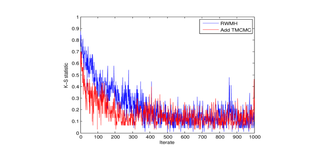
Refer to caption
(a) d=30,=2.4.formulae-sequence𝑑302.4d=30,~{}\ell=2.4.
Refer to caption
(b) d=30,=6.formulae-sequence𝑑306d=30,~{}\ell=6.
Figure 10: K-S distance comparison before burn-in between the RWM and the TMCMC chains for dimension d=30𝑑30d=30.
Refer to caption
(a) d=100,=2.4.formulae-sequence𝑑1002.4d=100,~{}\ell=2.4.
Refer to caption
(b) d=100,=6.formulae-sequence𝑑1006d=100,~{}\ell=6.
Figure 11: K-S distance comparison before burn-in between the RWM and the TMCMC chains for dimension d=100𝑑100d=100.

7.2 Comparisons between additive TMCMC and RWM in the independent, but non-identical set-up

We now compare additive TMCMC with RWM under an instance of independent, but non-identical situation provided in Bédard (2008a). In particular, we assume the target distribution to have independent normal components with all the means zero, and variances given by θ2(d)=(d1/5,d1/5,3,d0.5,3,d0.5,,3,d0.5)superscript𝜃2𝑑superscript𝑑15superscript𝑑153superscript𝑑0.53superscript𝑑0.53superscript𝑑0.5\theta^{-2}(d)=(d^{-1/5},d^{-1/5},3,d^{-0.5},3,d^{-0.5},\ldots,3,d^{-0.5}). For our purpose, we set d=50𝑑50d=50 and implement 30 chains each for additive TMCMC and RWM, each chain run for 10,0001000010,000 iterations. For any given iteration, and for both TMCMC and RWM, we then compute the K-S distances based on the 30 chains, which are then compared.

Note that θ2(d)superscript𝜃2𝑑\theta^{-2}(d) consists of three forms of coordinates, namely, θ2(d)=3superscript𝜃2𝑑3\theta^{-2}(d)=3, θ2(d)=d0.5superscript𝜃2𝑑superscript𝑑0.5\theta^{-2}(d)=d^{-0.5}, and θ2(d)=d15superscript𝜃2𝑑superscript𝑑15\theta^{-2}(d)=d^{-\frac{1}{5}}. These are associated with three distinct marginal target densities. In the figures below, for these three distinct marginals, we separately compare TMCMC and RWM using K-S distances. That is, Figures 12, 13 and 14 compare TMCMC and RWM when θ2(d)=3superscript𝜃2𝑑3\theta^{-2}(d)=3, θ2(d)=d0.5superscript𝜃2𝑑superscript𝑑0.5\theta^{-2}(d)=d^{-0.5}, and θ2(d)=d15superscript𝜃2𝑑superscript𝑑15\theta^{-2}(d)=d^{-\frac{1}{5}}, respectively.

All the three instances, Figures 12, 13 and 14, clearly demonstrate the superiority of additive TMCMC over RWM.
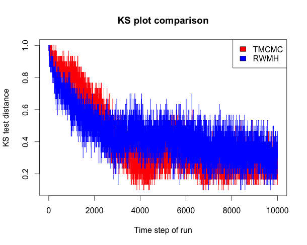
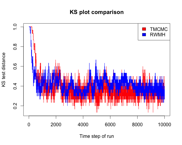
Refer to caption
Figure 12: Independent but non-identical case: K-S comparisons between additive TMCMC and RWM for θ2(d)=3superscript𝜃2𝑑3\theta^{-2}(d)=3.
Refer to caption
Figure 13: Independent but non-identical case: K-S comparisons between additive TMCMC and RWM for θ2(d)=d0.5superscript𝜃2𝑑superscript𝑑0.5\theta^{-2}(d)=d^{-0.5}.
Refer to caption
Figure 14: Independent but non-identical case: K-S comparisons between additive TMCMC and RWM for θ2(d)=d15superscript𝜃2𝑑superscript𝑑15\theta^{-2}(d)=d^{-\frac{1}{5}}.

7.3 Comparisons between additive TMCMC and RWM in the dependent set-up

We now compare additive TMCMC and RWM in the dependent set-up, as (46). That is, here we consider target densities of the type

πd(xd)=exp(xdTMdxd)i=1d1λiϕ(xiλi).subscript𝜋𝑑subscript𝑥𝑑superscriptsubscript𝑥𝑑𝑇subscript𝑀𝑑subscript𝑥𝑑superscriptsubscriptproduct𝑖1𝑑1subscript𝜆𝑖italic-ϕsubscript𝑥𝑖subscript𝜆𝑖\pi_{d}(x_{d})=\exp(-x_{d}^{T}M_{d}x_{d})\prod_{i=1}^{d}\frac{1}{\lambda_{i}}\phi\left(\frac{x_{i}}{\lambda_{i}}\right).

For our purpose, we consider the following forms of 𝝀=(λ1,,λd)𝝀subscript𝜆1subscript𝜆𝑑\boldsymbol{\lambda}=(\lambda_{1},\ldots,\lambda_{d}) and Mdsubscript𝑀𝑑M_{d}:

𝝀=α(1,1d,1d2,,1dd),𝝀𝛼11𝑑1superscript𝑑21superscript𝑑𝑑\boldsymbol{\lambda}=\alpha\left(1,\frac{1}{d},\frac{1}{d^{2}},\cdots,\frac{1}{d^{d}}\right),

and

Md=γ(1ρ)𝐈𝐝+ρ𝟏𝐝𝟏𝐝𝐓,subscript𝑀𝑑𝛾1𝜌subscript𝐈𝐝𝜌subscript1𝐝subscriptsuperscript1𝐓𝐝M_{d}=\gamma(1-\rho)\bf{I}_{d}+\rho\boldsymbol{1}_{d}\boldsymbol{1}^{T}_{d},

where 𝐈𝐝subscript𝐈𝐝\bf{I}_{d} is the identity matrix of order d𝑑d and 𝟏dsubscript1𝑑\boldsymbol{1}_{d} is the d𝑑d-component vector with all elements 111. We report the results of our experiments with three set-ups: (a) ρ=0.3𝜌0.3\rho=0.3, α=0.1𝛼0.1\alpha=0.1, γ=100𝛾100\gamma=100; (b) ρ=0.3𝜌0.3\rho=0.3, α=0.01𝛼0.01\alpha=0.01, γ=100𝛾100\gamma=100, and (c) ρ=0.3𝜌0.3\rho=0.3, α=0.01𝛼0.01\alpha=0.01, γ=1000𝛾1000\gamma=1000. The corresponding K-S based comparisons are provided in Figures 15, 16 and 17. In all the three experiments TMCMC very convincingly outperforms RWM. With various other choices of ρ𝜌\rho, α𝛼\alpha and γ𝛾\gamma we observed similar results (not reported due to lack of space).
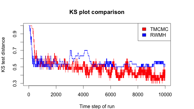
Refer to caption
Figure 15: Dependent case: K-S comparisons between additive TMCMC and RWM for ρ=0.3𝜌0.3\rho=0.3, α=0.1𝛼0.1\alpha=0.1, γ=100𝛾100\gamma=100.
Refer to caption
Figure 16: Dependent case: K-S comparisons between additive TMCMC and RWM for ρ=0.3𝜌0.3\rho=0.3, α=0.01𝛼0.01\alpha=0.01, γ=100𝛾100\gamma=100.
Refer to caption
Figure 17: Dependent case: K-S comparisons between additive TMCMC and RWM for ρ=0.3𝜌0.3\rho=0.3, α=0.01𝛼0.01\alpha=0.01, γ=1000𝛾1000\gamma=1000.

7.4 Discussion on simulation studies with multivariate Cauchy and multivariate t𝑡t as target densities

We have so far restricted ourselves to comparisons between TMCMC and RWM when the target distribution is Gaussian (i.i.d.formulae-sequence𝑖𝑖𝑑i.i.d., independent but non-identical, and dependent). However, Dey and Bhattacharya (2016b) conduct comparative studies between the two algorithms when the targets are multivariate Cauchy and multivariate t𝑡t. Briefly, they compare the algorithms with respect to K-S distance, when the location vectors and scale matrices are 𝝁=𝟎d𝝁subscript0𝑑\boldsymbol{\mu}=\boldsymbol{0}_{d} and 𝚺=diag{0.7𝟏d}+0.3𝟏d𝟏d𝚺𝑑𝑖𝑎𝑔0.7superscriptsubscript1𝑑0.3subscript1𝑑superscriptsubscript1𝑑\boldsymbol{\Sigma}=diag\{0.7\boldsymbol{1}_{d}^{\prime}\}+0.3\boldsymbol{1}_{d}\boldsymbol{1}_{d}^{\prime}, respectively, where 𝟎dsubscript0𝑑\boldsymbol{0}_{d} is a d𝑑d-dimensional vector with all elements 00. For multivariate t𝑡t, they choose ν=10𝜈10\nu=10 degrees of freedom. For both RWMH and additive TMCMC they consider the scale of the proposal distribution to be 2.4, and illustrate the methods for dimension d=50𝑑50d=50.

In fact, they compare the performances of RWM and additive TMCMC by two methods. In one method, since the above-mentioned target densities are not in the super-exponential family (see Dey and Bhattacharya (2016b) and the references therein), they transform them to superexponential distributions using a diffeomorphism proposed by Johnson and Geyer (2012), obtain samples from the transformed target densities using RWM and TMCMC, and then give inverse transformations to the simulated values so that they finally represent the original multivariate Cauchy and multivariate t𝑡t. The other method is direct application of the algorithms to the original targets. In other words, Dey and Bhattacharya (2016b) also apply RWM and TMCMC directly to multivariate Cauchy and multivariate t𝑡t, without resorting to diffeomorphism, and compare their performances. However, they also note that there are substantial gains with respect to mixing properties in the diffeomorphism based approach.

In either case, Dey and Bhattacharya (2016b) demonstrate that additive TMCMC outperforms RWM quite significantly in the case of the dependent, high-dimensional target densities. They even compare their performances in the case of i.i.d.formulae-sequence𝑖𝑖𝑑i.i.d. Cauchy and t𝑡t (with ν=10𝜈10\nu=10 degrees of freedom) distributions and reach the same conclusions.

8 Comparison of additive TMCMC and RWM in the case of a real, spatial data set

We now compare additive TMCMC and RWM with respect to a real, spatial dataset on radionuclide count data on Rongelap Island, analysed by Diggle et al. (1998) using a Bayesian hierarchical spatial model. This dataset and the model has been used subsequently by Christensen (2006) and Dutta and Bhattacharya (2014), to evaluate performances of Metropolis-Hastings and TMCMC algorithms, respectively.

8.1 Model and prior specification

For i=1,,157𝑖1157i=1,\ldots,157, Diggle et al. (1998) model the radionuclide count data as

YiPoisson(Mi),similar-tosubscript𝑌𝑖𝑃𝑜𝑖𝑠𝑠𝑜𝑛subscript𝑀𝑖Y_{i}\sim Poisson(M_{i}),

where

Mi=tiexp{β+S(𝕩i)};subscript𝑀𝑖subscript𝑡𝑖𝛽𝑆subscript𝕩𝑖M_{i}=t_{i}\exp\{\beta+S(\mathbb{x}_{i})\};

tisubscript𝑡𝑖t_{i} is the duration of observation at location 𝕩isubscript𝕩𝑖\mathbb{x}_{i}, β𝛽\beta is an unknown parameter and S()𝑆S(\cdot) is a zero-mean Gaussian process with isotropic covariance function of the form

Cov(S(𝕫1),S(𝕫2))=σ2exp{(α𝕫1𝕫2)δ}𝐶𝑜𝑣𝑆subscript𝕫1𝑆subscript𝕫2superscript𝜎2superscript𝛼normsubscript𝕫1subscript𝕫2𝛿Cov\left(S(\mathbb{z}_{1}),S(\mathbb{z}_{2})\right)=\sigma^{2}\exp\{-\left(\alpha\parallel\mathbb{z}_{1}-\mathbb{z}_{2}\parallel\right)^{\delta}\}

for any two locations 𝕫1,𝕫2subscript𝕫1subscript𝕫2\mathbb{z}_{1},\mathbb{z}_{2}. In the above, \parallel\cdot\parallel denotes the Euclidean distance between two locations, and (σ2,α,δ)superscript𝜎2𝛼𝛿(\sigma^{2},\alpha,\delta) are unknown parameters. Following Christensen (2006) we set δ=1𝛿1\delta=1, and assume uniform priors on the entire parameter space corresponding to (β,log(σ2),log(α))𝛽superscript𝜎2𝛼(\beta,\log(\sigma^{2}),\log(\alpha)). Thus, there are 160160160 parameters to be updated in each iteration of additive TMCMC and RWM.

8.2 Optimal scaling

Note that the likelihood times the prior in this case can be approximately expressed as (46), that is, although the Poisson likelihood is expressible in the form exp(Ψd(xd))superscriptΨ𝑑superscript𝑥𝑑\exp(-\Psi^{d}(x^{d})), the Gaussian process prior for S()𝑆S(\cdot) does not of course admit the form i=1d1λiϕ(xiλi)superscriptsubscriptproduct𝑖1𝑑1subscript𝜆𝑖italic-ϕsubscript𝑥𝑖subscript𝜆𝑖\prod_{i=1}^{d}\frac{1}{\lambda_{i}}\phi\left(\frac{x_{i}}{\lambda_{i}}\right) because of its dependence structure. Hence, this is an instance of a target density which does not fall within the class of densities for which optimal scaling theory has been developed. As is recommended in general cases, one may attempt tuning the parameters to approximately achieve the optimal acceptance rate. But this is a difficult task because of the large dimensionality, as already discussed. A far more important cause for concern is that, even if one succeeds in approximating the optimal acceptance rate, the corresponding scales will generally still be sub-optimal, because of the existence of many solutions such that the optimal acceptance rate holds. Indeed, we devise a method for approximately obtaining the optimal acceptance rates, but show that the corresponding scales lead to really poor performance of RWM, while thanks to the robustness property of additive TMCMC, the latter yields much reasonable performance. Details follow.

8.2.1 Pilot TMCMC for facilitating approximate optimal scaling

We first consider a pilot TMCMC run consisting of 11×10611superscript10611\times 10^{6} iterations, with the same TMCMC algorithm used by Dutta and Bhattacharya (2014). In other words, for the pilot run we draw ϵN(0,1)𝕀(ϵ>0)similar-toitalic-ϵ𝑁01𝕀italic-ϵ0\epsilon\sim N(0,1)\mathbb{I}(\epsilon>0), and consider the following additive transformations:

T(β,ϵ)𝑇𝛽italic-ϵ\displaystyle T(\beta,\epsilon) =β±2ϵ,absentplus-or-minus𝛽2italic-ϵ\displaystyle=\beta\pm 2\epsilon,
T(log(σ2),ϵ)𝑇superscript𝜎2italic-ϵ\displaystyle T(\log(\sigma^{2}),\epsilon) =log(σ2)±5ϵ,absentplus-or-minussuperscript𝜎25italic-ϵ\displaystyle=\log(\sigma^{2})\pm 5\epsilon,
T(log(α),ϵ)𝑇𝛼italic-ϵ\displaystyle T(\log(\alpha),\epsilon) =log(α)±5ϵ,absentplus-or-minus𝛼5italic-ϵ\displaystyle=\log(\alpha)\pm 5\epsilon,
T(S(𝕩i),ϵ)𝑇𝑆subscript𝕩𝑖italic-ϵ\displaystyle T(S(\mathbb{x}_{i}),\epsilon) =S(𝕩i)±2ϵ;fori=1,,157,formulae-sequenceabsentplus-or-minus𝑆subscript𝕩𝑖2italic-ϵfor𝑖1157\displaystyle=S(\mathbb{x}_{i})\pm 2\epsilon;\ \ \mbox{for}\ \ i=1,\ldots,157,

where ``+"``"``+" and ``"``"``-" occur with probability 1/2121/2 each.

After discarding the first 106superscript10610^{6} iterations as burn-in, we then store one TMCMC sample in every 100100100 iterations to yield 105superscript10510^{5} thinned TMCMC realizations. With these stored realizations, we then obtain the empirical variance-covariance matrix of the 160160160 unknowns and store the 160160160 eigenvalues of the matrix.

8.2.2 Approximately optimal acceptance rates of additive TMCMC and RWM using the stored eigenvalues

For i=1,,160𝑖1160i=1,\ldots,160, letting θisubscript𝜃𝑖\theta_{i} denote the unknowns, and λisubscript𝜆𝑖\lambda_{i}, the corresponding eigenvalues, we then consider the following additive transformations for TMCMC:

T(θi,ϵ)=θi±cTMCMC2λiopt,TMCMC2dϵ,𝑇subscript𝜃𝑖italic-ϵplus-or-minussubscript𝜃𝑖subscript𝑐𝑇𝑀𝐶𝑀𝐶2subscript𝜆𝑖subscriptsuperscript2𝑜𝑝𝑡𝑇𝑀𝐶𝑀𝐶𝑑italic-ϵT(\theta_{i},\epsilon)=\theta_{i}\pm c_{TMCMC}\sqrt{\frac{2\lambda_{i}\ell^{2}_{opt,TMCMC}}{d}}\epsilon,

where ϵN(0,1)𝕀(ϵ>0)similar-toitalic-ϵ𝑁01𝕀italic-ϵ0\epsilon\sim N(0,1)\mathbb{I}(\epsilon>0), ``+"``"``+" and ``"``"``-" occur with probability 1/2121/2 each, opt,TMCMC=1.715subscript𝑜𝑝𝑡𝑇𝑀𝐶𝑀𝐶1.715\ell_{opt,TMCMC}=1.715 (see (72)), and cTMCMCsubscript𝑐𝑇𝑀𝐶𝑀𝐶c_{TMCMC} is a tuning parameter for adjusting the acceptance rate to about 44%percent4444\%. It turned out, after setting cTMCMC=0.95subscript𝑐𝑇𝑀𝐶𝑀𝐶0.95c_{TMCMC}=0.95, that the empirical acceptance rate obtained from a TMCMC run of length 1.01×1081.01superscript1081.01\times 10^{8}, after discarding the first 1.7×1071.7superscript1071.7\times 10^{7} iterations as burn-in, is very accurately approximated as 0.4390.4390.439. Implementing this TMCMC algorithm, we store one in every 100100100 realizations after the burn-in to obtain 8.5×1058.5superscript1058.5\times 10^{5} thinned additive TMCMC realizations from the posterior distribution. The total time for the implementation took 464646 hours and 515151 minutes on a 64 bit machine with CPU MHz 160016001600 and about 888 GB memory.

For RWM, we consider the following proposal:

T(θi,ϵi)=θi+cRWM2λiopt,RWM2dϵi,𝑇subscript𝜃𝑖subscriptitalic-ϵ𝑖subscript𝜃𝑖subscript𝑐𝑅𝑊𝑀2subscript𝜆𝑖subscriptsuperscript2𝑜𝑝𝑡𝑅𝑊𝑀𝑑subscriptitalic-ϵ𝑖T(\theta_{i},\epsilon_{i})=\theta_{i}+c_{RWM}\sqrt{\frac{2\lambda_{i}\ell^{2}_{opt,RWM}}{d}}\epsilon_{i},

where ϵi.i.d.N(0,1)\epsilon\stackrel{{\scriptstyle i.i.d.}}{{\sim}}N(0,1), opt,RWM=1.715subscript𝑜𝑝𝑡𝑅𝑊𝑀1.715\ell_{opt,RWM}=1.715, and cRWM=0.95=cTMCMCsubscript𝑐𝑅𝑊𝑀0.95subscript𝑐𝑇𝑀𝐶𝑀𝐶c_{RWM}=0.95=c_{TMCMC}. We obtain the empirical acceptance rate from a RWM run of length 1.01×1081.01superscript1081.01\times 10^{8}, after discarding the first 1.7×1071.7superscript1071.7\times 10^{7} iterations as burn-in, as approximately 0.2280.2280.228. We implement this RWM algorithm, storing one in every 100100100 realizations after the burn-in to obtain 8.5×1058.5superscript1058.5\times 10^{5} thinned RWM realizations from the posterior. The total time for the implementation took 464646 hours and 535353 minutes on the same machine on which TMCMC was implemented.

8.3 Results of comparison

Figures 18 and 19 show the trace plots of the stored realizations obtained by TMCMC and RWM, respectively, after a further thinning of size 300300300. Such substantial further thinning is required to facilitate effortless visual comparison of the autocorrelation plots for TMCMC and RWM shown in Figure 20. In Figures 18 and 19 it is worth observing that, RWM, composed of 160160160 ϵisubscriptitalic-ϵ𝑖\epsilon_{i}’s in this example, is prone to require a large number of iterations to return to any given set with positive posterior probability, once it leaves it. On the other hand, TMCMC marches off to convergence much faster than RWM, exploiting its more localized move types thanks to a single ϵitalic-ϵ\epsilon. This insight is more formalized by the comparison of the associated autocorrelation plots shown in Figure 20. It is obvious that TMCMC significantly outperforms RWM in terms of autocorrelations in all the cases.

Since scaling is directly related to autocorrelation (see Sections S-3 and S-4 of the supplement), it is clear that poor scaling of RWM in comparison with additive TMCMC is the reason for the relatively poor performance of the former. Indeed, even though we could approximately achieve the desired acceptance rates, there are many solutions for the scales, given the same acceptance rate; in fact, selecting reasonable scales gets increasing difficult with increasing dimensions. Thus, it is highly unlikely that the chosen scales are even reasonable in this high-dimensional example, for either TMCMC or RWM. As a result it makes sense to conclude with respect to the autocorrelations that, in this real data study, sensitivity of RWM with respect to optimal scales is the reason for its relatively poor performance, while robustness of TMCMC in this regard is the reason for its quite reasonable performance.

Thus, in this real data example, additive TMCMC very clearly and very convincingly outperforms RWM.

Refer to caption
(a) Trace plot of α𝛼\alpha.
Refer to caption
(b) Trace plot of β𝛽\beta.
Refer to caption
(c) Trace plot of σ2superscript𝜎2\sigma^{2}.
Refer to caption
(d) Trace plot of S(𝕩1)𝑆subscript𝕩1S(\mathbb{x}_{1}).
Refer to caption
(e) Trace plot of S(𝕩10)𝑆subscript𝕩10S(\mathbb{x}_{10}).
Refer to caption
(f) Trace plot of S(𝕩50)𝑆subscript𝕩50S(\mathbb{x}_{50}).
Refer to caption
(g) Trace plot of S(𝕩100)𝑆subscript𝕩100S(\mathbb{x}_{100}).
Refer to caption
(h) Trace plot of S(𝕩150)𝑆subscript𝕩150S(\mathbb{x}_{150}).
Refer to caption
(i) Trace plot of S(𝕩157)𝑆subscript𝕩157S(\mathbb{x}_{157}).
Figure 18: Rongelap island data: TMCMC based trace plots.
Refer to caption
(a) Trace plot of α𝛼\alpha.
Refer to caption
(b) Trace plot of β𝛽\beta.
Refer to caption
(c) Trace plot of σ2superscript𝜎2\sigma^{2}.
Refer to caption
(d) Trace plot of S(𝕩1)𝑆subscript𝕩1S(\mathbb{x}_{1}).
Refer to caption
(e) Trace plot of S(𝕩10)𝑆subscript𝕩10S(\mathbb{x}_{10}).
Refer to caption
(f) Trace plot of S(𝕩50)𝑆subscript𝕩50S(\mathbb{x}_{50}).
Refer to caption
(g) Trace plot of S(𝕩100)𝑆subscript𝕩100S(\mathbb{x}_{100}).
Refer to caption
(h) Trace plot of S(𝕩150)𝑆subscript𝕩150S(\mathbb{x}_{150}).
Refer to caption
(i) Trace plot of S(𝕩157)𝑆subscript𝕩157S(\mathbb{x}_{157}).
Figure 19: Rongelap island data: RWM based trace plots.
Refer to caption
(a) ACF comparison for α𝛼\alpha.
Refer to caption
(b) ACF comparison for β𝛽\beta.
Refer to caption
(c) ACF comparison for σ2superscript𝜎2\sigma^{2}.
Refer to caption
(d) ACF comparison for S(𝕩1)𝑆subscript𝕩1S(\mathbb{x}_{1}).
Refer to caption
(e) ACF comparison for S(𝕩10)𝑆subscript𝕩10S(\mathbb{x}_{10}).
Refer to caption
(f) ACF comparison for S(𝕩50)𝑆subscript𝕩50S(\mathbb{x}_{50}).
Refer to caption
(g) ACF comparison for S(𝕩100)𝑆subscript𝕩100S(\mathbb{x}_{100}).
Refer to caption
(h) ACF comparison for S(𝕩150)𝑆subscript𝕩150S(\mathbb{x}_{150}).
Refer to caption
(i) ACF comparison for S(𝕩157)𝑆subscript𝕩157S(\mathbb{x}_{157}).
Figure 20: Rongelap island data: Comparisons of the ACF’s based on TMCMC and RWM. The TMCMC-based ACF’s are depicted by the green colour and the red colour is associated with RWM-based ACF’s.

9 Conclusion

Overall, our assessment is that TMCMC is clearly advantageous compared to RWM from various perspectives. It has significantly less computational complexity and the acceptance rate corresponding to the optimal scaling for TMCMC (0.439) is almost twice that of RWM (0.234). Although the maximum diffusion speed of RWM is somewhat higher than that of additive TMCMC, the latter is much more robust with respect to misspecifications of the scales. The advantages of such robustness are spelt out in the discussions in Sections S-3 and S-4 of the supplement. Our simulation studies reported in Section 7 and Table 1, and the real data analysis in Section 8, clearly vindicate these discussions.

Related to the discussions on robustness and the difficulty of choosing proper scalings in high dimensions is also the issue of increasing computational complexity, particularly in the Bayesian paradigm. Note that complex, high-dimensional posteriors routinely arise in Bayesian applications. It is extremely uncommon among MCMC practitioners to use the RWM algorithm for updating all the parameters in a single block associated with any significantly high-dimensional posterior arising from any complex Bayesian application. We presume that the extreme difficulty of determining proper scalings in practice prevent the researchers from using the RWM as an algorithm for updating all the parameters in a single block. Indeed, as we demonstrated with our simulation study reported in Table 1, misspecification even in the case of the simple target distribution being a product of i.i.d.formulae-sequence𝑖𝑖𝑑i.i.d. normal densities, leads to acceptance rates that are almost zero. In the context of the real data study in Section 8 we proposed a method for approximately obtaining the presumed optimal acceptance rates, and which appears to be generally applicable, but as we demonstrated, RWM failed to exhibit adequate mixing properties. Adaptive strategies may be thought of as alternative methods, but these are yet to gain enough popularity among applied MCMC practitioners; moreover, as we mention in Section S-5 of the supplement, extremely long runs may be necessary to reach adequate acceptance rates for adaptive RWM, which may be prohibitive in very high dimensions, for example, when the acceptance ratio involves high-dimensional matrix inversions at every iteration, such as in our spatial example.

The aforementioned difficulties force the researchers to use RWM to sequentially update the parameters, either singly, or in small blocks. Since one (or just a few) parameters are updated at a time by RWM, the acceptance rate can be controlled at each stage of the sequential updating procedure. However, this sequential procedure also requires computation of the acceptance ratio as many times as every small block is updated in a sequence. If each parameter is updated singly (that is, each small block consists of only one element), then the computational complexity increases d𝑑d-folds compared to the procedure where all the d𝑑d parameters are updated in a single block. Thus, when d𝑑d is large, the computation can become prohibitively slow.

On the other hand, TMCMC is designed to update all the parameters in a single block in such a way that the acceptance rate remains reasonable in spite of the high dimensionality and complexity of the target distribution. Our simulation studies and real data example in Section 8 show that misspecification of the scales do not have drastic effect on the efficiency of additive TMCMC, thanks to its robustness property. As a result, with much less effort compared to that required for RWM, we can achieve reasonable scalings that ensure adequate performance of additive TMCMC, so that resorting to sequential updating will not be necessary.

This also implies that unlike RWM, additive TMCMC can save enormous computational effort when the dimension d𝑑d is large. Finally, adaptive TMCMC may be of much value in very high dimensions because of its quick convergence to the correct optimal acceptance rate, and for ensuring good performance. The details will be covered in Dey and Bhattacharya (2015).

Our empirical findings reported in this article with respect to the simulation studies pertaining to i.i.d.formulae-sequence𝑖𝑖𝑑i.i.d., independent but non-identical, as well as dependent cases clearly point towards supremacy of TMCMC over RWM. Quite importantly, in the real, spatial data example, TMCMC outperformed RWM very significantly. Indeed, even though we could tune the scales so as to achieve approximately the respective optimal acceptance rates, the chosen scales need not be actually optimal, for either of TMCMC and RWM. Here RWM is convincingly outperformed by TMCMC thanks to its remarkably robust nature with respect to the choice of scales. Thus, all our experiments, particularly, the challenging real data example, lead us to clearly recommend TMCMC in general situations.

Given the importance of the general TMCMC idea, we have decided to create a software for its general usage. In this regard, we have now made available an R package tmcmcR for implementing TMCMC along with its adaptive versions at the Github page

𝐡𝐭𝐭𝐩𝐬://𝐠𝐢𝐭𝐡𝐮𝐛.𝐜𝐨𝐦/𝐤𝐤𝐝𝐞𝐲/𝐭𝐦𝐜𝐦𝐜𝐑.{\bf https://github.com/kkdey/tmcmcR}.

The software will be continuously updated in accordance with further developments of TMCMC; moreover, TTMCMC, the variable-dimensional version of TMCMC, will also be incorporated, and kept updated.

As part of our future work, we plan to extend TMCMC to multiple-try TMCMC, and investigate the corresponding optimal scaling theory. By multiple-try TMCMC we mean the TMCMC algorithm that selects the next proposal from a set of available, perhaps dependent, proposals. For MH-adapted versions of such an idea, see, for example, Liu et al. (2000) and Liang et al. (2010), Martino and Read (2013). Bédard et al. (2012) investigated scaling analysis of such methods in the MH context. The advantages of TMCMC over MH quite reasonably lead us to expect substantial gains of multiple-try TMCMC over multiple-try MH.

Acknowledgment

We are sincerely grateful to the two reviewers for very encouraging and constructive comments which helped substantially improve the quality and presentation of our manuscript.

Supplementary Material

Throughout, we refer to our main manuscript Dey and Bhattacharya (2016a) as DB.

S-1 Computational efficiency of TMCMC

It may seem that TMCMC is computationally more expensive because we are randomly generating d+1𝑑1d+1 many values (ϵ,b1,b2,,bd)italic-ϵsubscript𝑏1subscript𝑏2subscript𝑏𝑑(\epsilon,b_{1},b_{2},\ldots,b_{d}) whereas in RWM, we are generating d𝑑d many random variables (ϵ1,ϵ2,,ϵd)subscriptitalic-ϵ1subscriptitalic-ϵ2subscriptitalic-ϵ𝑑(\epsilon_{1},\epsilon_{2},\ldots,\epsilon_{d}) where ϵN(0,2d)I{ϵ>0}similar-toitalic-ϵ𝑁0superscript2𝑑subscript𝐼italic-ϵ0\epsilon\sim N(0,\frac{\ell^{2}}{d})I_{\{\epsilon>0\}} and ϵiN(0,2d)i=1,2,,dformulae-sequencesimilar-tosubscriptitalic-ϵ𝑖𝑁0superscript2𝑑for-all𝑖12𝑑\epsilon_{i}\sim N(0,\frac{\ell^{2}}{d})~{}\forall~{}i=1,2,\ldots,d. However generating bisubscript𝑏𝑖b_{i} is equivalent to simple tosses of a fair coin which is a much easier exercise compared to drawing a set of independent normal random variables required by RWM. As a vindication of this, we obtain the average computation time (in seconds) of 100,00,00 iterations with RWM and TMCMC algorithms across dimensions 2 to 100, averaged over 100 replications of 100,00,00 iterations for each dimension, when the d𝑑d-dimensional target density is a product of d𝑑d standard normals. The codes are written in C and implemented in an ordinary 32-bit laptop. The results of our experiment are displayed in Figure S-1. Fgure S-2 displays the computation times of RWM and TMCMC with respect to a single replication of the 100,00,00 iterations. In both the diagrams, TMCMC is seen to take significantly less computational time compared to the RWM algorithm, particularly in higher dimensions. Much longer runs, particularly in very high dimensions, would see TMCMC saving very substantial amount of computational time in comparison with RWM. For further discussion on computational gains of TMCMC over RWM, see Section 9 of DB.
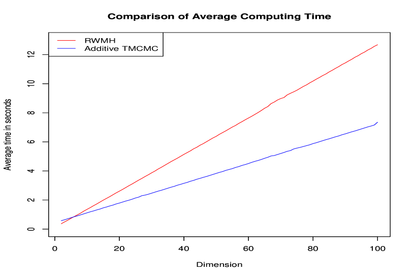
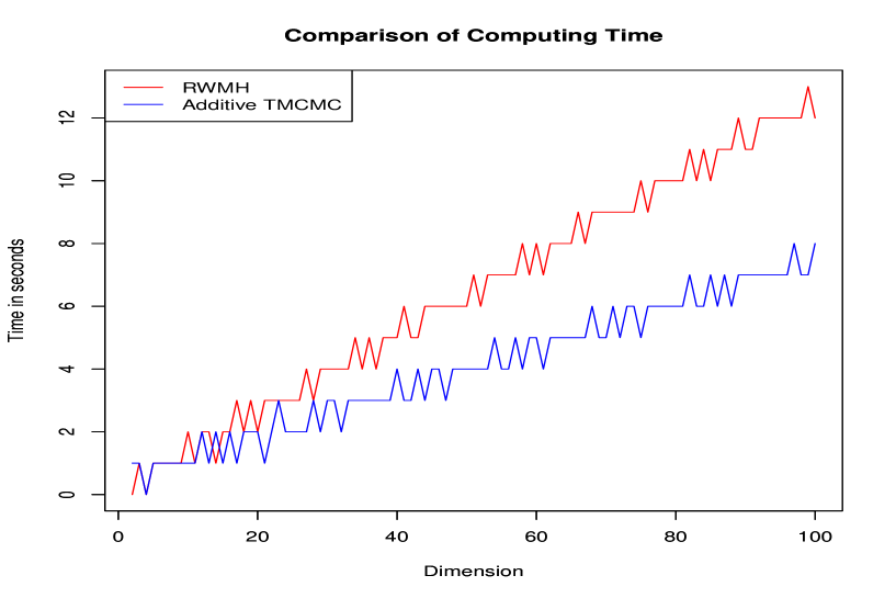
Refer to caption
Figure S-1: Average computation time (in seconds) of 100,00,00 iterations with RWM and TMCMC algorithms corresponding to dimensions varying from 2 to 100. TMCMC takes significantly less computation time compared to RWM, particularly in higher dimensions. The codes are written in C and implemented on an ordinary 32-bit laptop.
Refer to caption
Figure S-2: Computation time (in seconds) of 100,00,00 iterations with RWM and TMCMC algorithms corresponding to dimensions varying from 2 to 100. TMCMC takes significantly less computation time compared to RWM, particularly in higher dimensions. The codes are written in C and implemented on an ordinary 32-bit laptop.

It must be emphasized that the proposal density for ϵitalic-ϵ\epsilon in TMCMC can be any distribution on the positive support. Similarly, the RWM algorithm also does not require the proposal to be normal. However, the optimal scaling results for RWM inherently assume normality and for the sake of comparison, we have also restricted our focus on ϵN(0,2d)I{ϵ>0}similar-toitalic-ϵ𝑁0superscript2𝑑subscript𝐼italic-ϵ0\epsilon\sim N(0,\frac{\ell^{2}}{d})I_{\{\epsilon>0\}} in the subsequent sections.

S-2 Details on the need for optimal scaling of additive TMCMC

We first try to impress the fact that too small or too large values of \ell can both lead to poor performance of the chain and it is this trade-off that draws our interest in finding an optimal value of \ell. If the value of \ell or equivalently, the proposal variance, is large, then the probability of a move falling in low density regions (with respect to the target density) of the space increases as the moves (x1+b1ϵ,,xd+bdϵ)subscript𝑥1subscript𝑏1italic-ϵsubscript𝑥𝑑subscript𝑏𝑑italic-ϵ(x_{1}+b_{1}\epsilon,\ldots,x_{d}+b_{d}\epsilon) are likely to be quite far apart from (x1,,xd)subscript𝑥1subscript𝑥𝑑(x_{1},\ldots,x_{d}). This leads to smaller values of the ratio π(x1+b1ϵ,,xd+bdϵ)π(x1,,xd)𝜋subscript𝑥1subscript𝑏1italic-ϵsubscript𝑥𝑑subscript𝑏𝑑italic-ϵ𝜋subscript𝑥1subscript𝑥𝑑\frac{\pi(x_{1}+b_{1}\epsilon,\ldots,x_{d}+b_{d}\epsilon)}{\pi(x_{1},\ldots,x_{d})} and thus lower acceptance rates. In fact, for high dimensions, this acceptance rate can be quite low for even moderately large values of \ell. On the other hand, if the value of \ell is too small, then the acceptance rate will be higher but we then have to compromise in terms of exploration of the space. Much of our moves will lie very close to the initial point and as a result, the chain will move very slowly. An instance of the movement of the RWM and additive TMCMC chain for significantly small and large values of \ell are depicted in Figure S-3 assuming that the target distribution is standard normal. For small values of \ell, the fact that the chain moves slowly gets reflected in the autocorrelation factor (ACF) of the chain, which would be on the higher side (Figure S-4). All these motivate us to find an optimal value of \ell that would take care of these problems. Our approach would be to derive the diffusion process approximation of the additive TMCMC process in the limit as d𝑑d\rightarrow\infty and then we maximize the diffusion speed or the rate of change of variance of the chain in the limit. Intuitively, if the scale factor \ell is small, then starting from a point Xtsubscript𝑋𝑡X_{t} at time t𝑡t, the moves corresponding to adjacent time points Xt+hsubscript𝑋𝑡X_{t+h} are quite close and so the limiting change of variation is quite small for the corresponding diffusion process. If on the other hand the scale factor \ell is large, the chain hardly moves, and hence Xt+hsubscript𝑋𝑡X_{t+h} for sufficiently small hh are often same as Xtsubscript𝑋𝑡X_{t}, thereby leading to lower value of diffusion speed. On optimizing the diffusion speed for the TMCMC chain, we obtain the optimal value of the acceptance rate to be 0.439. Panels (a), (b) and (c) of Figure S-5 depict the path of the TMCMC chain for various choices of proposal variance, ranging from too small through the optimal value to quite large. Note that the target density is best approximated by the chain at optimal scaling. A better understanding of this is achieved by perceiving how well the histogram of observations obtained after running a chain up to a certain length of time, approximates the true density (panels (c), (d), (e) of Figure S-5).

Refer to caption
(a) Sample paths of RWM and additive TMCMC for small proposal variance.
Refer to caption
(b) Sample paths of RWM and additive TMCMC for large proposal variance.
Figure S-3: Comparison of RWM and additive TMCMC sample paths for small and large values of the proposal variance. The target density is N(0,1)𝑁01N(0,1), the standard normal distribution.
Refer to caption
Figure S-4: ACFs of RWM and additive TMCMC for small proposal variance. The target density is N(0,1)𝑁01N(0,1), the standard normal distribution.
Refer to caption
(a) =0.010.01\ell=0.01
Refer to caption
(b) =2.4(optimal)2.4optimal\ell=2.4~{}(\mbox{optimal})
Refer to caption
(c) =2020\ell=20
Refer to caption
(d) =0.010.01\ell=0.01
Refer to caption
(e) =2.4(optimal)2.4optimal\ell=2.4~{}(\mbox{optimal})
Refer to caption
(f) =2020\ell=20
Figure S-5: The upper panels (a), (b) and (c) show the paths of TMCMC chain for three various choices of scalings together with the target density N(0,1)𝑁01N(0,1) plot. These highlight how well the paths explore the given target density. The lower panels (c), (d) and (e) display the histograms of the sample observations obtained from TMCMC for these choices of scalings together with the target density N(0,1)𝑁01N(0,1). These highlight how well the histograms approximate the target density for the given run of TMCMC.

S-3 Discussion on consequences of non-robustness of RWM with respect to scale choices

For general, d𝑑d-dimensional target distributions, RWM entails the proposal with transitions of the form (x1,,xd)(x1+1dϵ1,,x1+ddϵd)subscript𝑥1subscript𝑥𝑑subscript𝑥1subscript1𝑑subscriptitalic-ϵ1subscript𝑥1subscript𝑑𝑑subscriptitalic-ϵ𝑑(x_{1},\ldots,x_{d})\rightarrow(x_{1}+\frac{\ell_{1}}{\sqrt{d}}\epsilon_{1},\ldots,x_{1}+\frac{\ell_{d}}{\sqrt{d}}\epsilon_{d}), where, for i=1,,d𝑖1𝑑i=1,\ldots,d, ϵiN(0,1)similar-tosubscriptitalic-ϵ𝑖𝑁01\epsilon_{i}\sim N(0,1), and isubscript𝑖\ell_{i} are constants to be chosen appropriately. Often isubscript𝑖\ell_{i} may be of the form aisubscript𝑎𝑖\ell a_{i}, where aisubscript𝑎𝑖a_{i} may be needed to determine appropriately in addition to \ell. As instance of this form occurs in the dependent set-up of Mattingly et al. (2011), but aisubscript𝑎𝑖a_{i} in that set-up are the square roots of the eigenvalues of the Gaussian measure with independent components that is assumed to dominate the target density. However, in practice such assumption of independent Gaussian components will generally not hold, and hence it is far from straightforward to determine aisubscript𝑎𝑖a_{i} appropriately in realistic cases.

Since all the set-ups considered so far yield the optimal acceptance rate 0.234 for RWM, it may be anticipated that the result holds quite generally, and applied MCMC practitioners may be advised to tune (1,,d)subscript1subscript𝑑(\ell_{1},\ldots,\ell_{d}) such that the acceptance rate is close to 0.234. In fact, using a measure of efficiency which is the reciprocal of integrated autocorrelation time, Roberts and Rosenthal (2001) demonstrate that the RWM proposal may be tuned to achieve an acceptance rate between 0.15 to 0.5, which would make the algorithm around 80% efficient. However, for large dimension d𝑑d, appropriate tuning of so many scale parameters seems to be an extremely arduous task. In our simulations presented in Section 8 of DB we observe that even in the simple situation where the target density is an iid𝑖𝑖𝑑iid product of normal densities, when the dimension increases, particularly when d=100𝑑100d=100 and d=200𝑑200d=200, departure from the optimal scale results in drastic fall in acceptance rates, far below what is prescribed by Roberts and Rosenthal (2001); see Table 1 of DB. The diffusion speeds under such mis-specifications tend to be quite low because of non-robustness with respect to scale choice (see Figures 1 – 6 of DB). Since low diffusion speed is equivalent to high autocorrelation (see equation (18) of Roberts and Rosenthal (2001)), the efficiency measures of Roberts and Rosenthal (2001) that use integrated autocorrelation, are also expected to indicate less efficiency. Thus, in summary manually tuning the RWM proposals appropriately in more general and complicated situations and in high dimensions seems to be a very daunting task. There are methods for automatically and adaptively tuning the scales to progress towards the desired optimal acceptance rate as number of iterations increases, but as we discuss in Section S-5 computationally this can be a very costly exercise in high dimensions.

S-4 Discussion on possible advantages of additive TMCMC for relatively more robust behaviour with respect to scale choices

Our results on optimal scaling offers the following general thumb rule to the users of additive TMCMC: tune the additive TMCMC proposal to achieve approximately 44% acceptance rate. Note that even though the optimal acceptance rate of additive TMCMC is significantly higher than that of RWM, both the algorithms have approximately the same optimal scalings that maximize the diffusion speeds (see Figures 1 – 6).

The results of our simulation studies reported in Table 1 of DB demonstrate that even in dimension as low as d=2𝑑2d=2, our optimal acceptance rate 0.439 is remarkably accurate. The table further demonstrates that even if the scale of additive TMCMC is sub-optimally chosen, the acceptance rates remain higher than 20% for all dimensions, whereas for the same sub-optimal scale choice the acceptance rate of RWM falls to about 0.33% in high dimensions. Figures 1 – 6 show that around the optimal scale, the diffusion speeds of additive TMCMC under various set-ups do not change significantly. Using the relationship between diffusion speed and the measure of efficiency proposed by Roberts and Rosenthal (2001) one can conclude that unlike RWM, the efficiency of additive TMCMC is not substantially affected by sub-optimal scale choices. Hence, tuning the additive TMCMC proposal is a far more safe and easy exercise compared to that of RWM. It seems to us that this is quite an advantage of additive TMCMC over RWM in general, high-dimensional set-ups. As we discuss in Section S-5 adaptive methods can be employed to approach the exact optimal acceptance rate 0.439 in substantially less number of iterations compared to adaptive RWM, facilitating huge computational gain over the latter.

S-5 Discussion on adaptive versions of RWM and additive TMCMC for enforcing optimal acceptance rates in complex, high-dimensional problems

Adaptive MCMC methods (see, for example, Roberts and Rosenthal (2009) and the references therein) are designed to combat the difficulty of determining appropriate proposal scalings. In the context of RWM, various adaptive strategies are presented in Roberts and Rosenthal (2009) to choose the scalings in an adaptive manner so that the optimal acceptance rate 0.234 is achieved in the long run. Dey and Bhattacharya (2015) adopted the strategies in the case of additive TMCMC and made a detailed comparison with the corresponding adaptive RWM methods. In particular, they found that even after a very large number of iterations most of the the adaptive methods related to RWM yielded acceptance rates which are significantly different from 0.234, while the adaptive TMCMC algorithms very quickly yielded acceptance rates reasonably close 0.439, even in dimensions as low as d=2𝑑2d=2. This implies quite substantial savings of TMCMC in terms of computation time in comparison with RWM. Performance wise as well, the results of Dey and Bhattacharya (2015) favour adaptive TMCMC over adaptive RWM in high dimensions, with respect to the various measures which we also employ in this current work.

S-6 Proofs of optimal scaling results of additive TMCMC

S-6.1 Proof of Theorem 3.1 of DB

Proof.

For our purpose, we define the discrete time generator of the TMCMC approach, as

GdV(x)subscript𝐺𝑑𝑉𝑥\displaystyle G_{d}{V(x)} =\displaystyle= d2d{bi{1,+1}i=1,,d}0[(V(x1+b1ϵ,,xd+bdϵ)V(x1,,xd))\displaystyle\frac{d}{2^{d}}\displaystyle\sum_{\left\{\begin{array}[]{l}b_{i}\in\{-1,+1\}\\ \forall i=1,\ldots,d\end{array}\right\}}\displaystyle\int_{0}^{\infty}\left[\left(\vphantom{min\left\{1,\frac{\pi(x_{1}+b_{1}\epsilon,\ldots,x_{d}+b_{d}\epsilon)}{\pi(x_{1},\ldots,x_{d})}\right\}}V\left(x_{1}+b_{1}\epsilon,\ldots,x_{d}+b_{d}\epsilon\right)-V\left(x_{1},\ldots,x_{d}\right)\right)\right.
×(min{1,π(x1+b1ϵ,,xd+bdϵ)π(x1,x2,,xd)})]q(ϵ)dϵ.\displaystyle\qquad\left.\hskip 85.35826pt\times\left(\normalsize\min\left\{1,\frac{\pi(x_{1}+b_{1}\epsilon,\ldots,x_{d}+b_{d}\epsilon)}{\pi(x_{1},x_{2},\ldots,x_{d})}\right\}\right)\right]q(\epsilon)d\epsilon.

Since by our assumption (logf)superscript𝑓(\log f)^{\prime} is Lipschitz, in the above equation we may assume that V𝑉V belongs to the space of infinitely differentiable functions with compact support (see, for example, Bédard (2007) for further details).

The Skorohod topology allows us to treat Gdsubscript𝐺𝑑G_{d} as a continuous time generator that has jumps at the rate d1superscript𝑑1d^{-1}. Given our restricted focus on a one dimensional component of the actual process, we assume V𝑉V to be a function of the first co-ordinate only. Under this assumption, the generator defined in (S-6.1) is a function of only ϵitalic-ϵ\epsilon and b1subscript𝑏1b_{1}, and can be rephrased as

GdV(x)subscript𝐺𝑑𝑉𝑥\displaystyle G_{d}{V(x)} =\displaystyle= d20b1{1,+1}[(V(x1+b1ϵ)V(x1))\displaystyle\frac{d}{2}\int_{0}^{\infty}\sum_{b_{1}\in\{-1,+1\}}\left[\left(\vphantom{\min\left\{1,\frac{\pi(x_{1}+b_{1}\epsilon,\ldots,x_{d}+b_{d}\epsilon)}{\pi(x_{1},\ldots,x_{d})}\right\}}V(x_{1}+b_{1}\epsilon)-V(x_{1})\right)\right.
×Eb2,,bd(min{1,π(x1+b1ϵ,,xd+bdϵ)π(x1,,xd)})]q(ϵ)dϵ,\displaystyle\qquad\quad\left.\hskip 56.9055pt\times E_{b_{2},\ldots,b_{d}}\left(\normalsize\min\left\{1,\frac{\pi(x_{1}+b_{1}\epsilon,\ldots,x_{d}+b_{d}\epsilon)}{\pi(x_{1},\ldots,x_{d})}\right\}\right)\right]q(\epsilon)d\epsilon,

where Eb2,,bdsubscript𝐸subscript𝑏2subscript𝑏𝑑E_{b_{2},\ldots,b_{d}} is the expectation taken conditional on b1subscript𝑏1b_{1} and ϵitalic-ϵ\epsilon.

First we show that the quantity GdV(x)subscript𝐺𝑑𝑉𝑥G_{d}V(x) is a bounded quantity.

GdV(x)subscript𝐺𝑑𝑉𝑥\displaystyle G_{d}{V(x)} \displaystyle\leq dE{b1,ϵ}[V(x1+b1ϵ)V(x1)]𝑑subscript𝐸subscript𝑏1italic-ϵdelimited-[]𝑉subscript𝑥1subscript𝑏1italic-ϵ𝑉subscript𝑥1\displaystyle dE_{\{b_{1},\epsilon\}}\left[V(x_{1}+b_{1}\epsilon)-V(x_{1})\right]
=\displaystyle= dV(x1)E{b1,ϵ}(b1ϵ)+d2V′′(x1)E{b1,ϵ}(ϵ2)𝑑superscript𝑉subscript𝑥1subscript𝐸subscript𝑏1italic-ϵsubscript𝑏1italic-ϵ𝑑2superscript𝑉′′subscriptsuperscript𝑥1subscript𝐸subscript𝑏1italic-ϵsuperscriptitalic-ϵ2\displaystyle dV^{{}^{\prime}}(x_{1})E_{\{b_{1},\epsilon\}}(b_{1}\epsilon)+\frac{d}{2}V^{{}^{\prime\prime}}(x^{*}_{1})E_{\{b_{1},\epsilon\}}(\epsilon^{2})
\displaystyle\leq 2K,superscript2𝐾\displaystyle\ell^{2}K,

where x1subscriptsuperscript𝑥1x^{*}_{1} lies between x1subscript𝑥1x_{1} and x1+b1ϵsubscript𝑥1subscript𝑏1italic-ϵx_{1}+b_{1}\epsilon and K𝐾K is the maximum value of V′′superscript𝑉′′V^{{}^{\prime\prime}}.

Note that

Eb2,,bdsubscript𝐸subscript𝑏2subscript𝑏𝑑\displaystyle E_{b_{2},\ldots,b_{d}} [min{1,π(x1+b1ϵ,,xd+bdϵ)π(x1,,xd)}]delimited-[]1𝜋subscript𝑥1subscript𝑏1italic-ϵsubscript𝑥𝑑subscript𝑏𝑑italic-ϵ𝜋subscript𝑥1subscript𝑥𝑑\displaystyle\left[\min\left\{1,\frac{\pi(x_{1}+b_{1}\epsilon,\ldots,x_{d}+b_{d}\epsilon)}{\pi(x_{1},\ldots,x_{d})}\right\}\right]
=\displaystyle= Eb2,,bd[min{1,exp(log(f(x1+b1ϵ))log(f(x1))\displaystyle E_{b_{2},\ldots,b_{d}}\left[\min\left\{1,\exp\left(\vphantom{\sum_{j=2}^{d}\left\{b_{j}\epsilon\left\{\log(f(x_{j}))\right\}^{{}^{\prime}}+\frac{\epsilon^{2}}{2!}\left\{\log(f(x_{j}))\right\}^{{}^{\prime\prime}}+\frac{b_{j}\epsilon^{3}}{3!}\left\{\log(f(z_{j}))\right\}^{{}^{\prime\prime\prime}}\right\}}\log(f(x_{1}+b_{1}\epsilon))-\log(f(x_{1}))\right.\right.\right.
+j=2d{bjϵ{log(f(xj))}+ϵ22!{log(f(xj))}′′+bjϵ33!{log(f(xj))}′′′+ϵ44!{log(f(zj))}′′′′})}],\displaystyle\left.\left.\left.+\sum_{j=2}^{d}\left\{b_{j}\epsilon\left\{\log(f(x_{j}))\right\}^{{}^{\prime}}+\frac{\epsilon^{2}}{2!}\left\{\log(f(x_{j}))\right\}^{{}^{\prime\prime}}+\frac{b_{j}\epsilon^{3}}{3!}\left\{\log(f(x_{j}))\right\}^{{}^{\prime\prime\prime}}+\frac{\epsilon^{4}}{4!}\left\{\log(f(z_{j}))\right\}^{{}^{\prime\prime\prime\prime}}\right\}\right)\right\}\right],

where Eb2,,bdsubscript𝐸subscript𝑏2subscript𝑏𝑑E_{b_{2},\ldots,b_{d}} denotes expectation with respect to b2,,bdsubscript𝑏2subscript𝑏𝑑b_{2},\ldots,b_{d}, holding ϵitalic-ϵ\epsilon, b1subscript𝑏1b_{1}, x1subscript𝑥1x_{1}, xjsubscript𝑥𝑗x_{j} and zjsubscript𝑧𝑗z_{j} (j=2,,d𝑗2𝑑j=2,\ldots,d) fixed; and for j=2,,d𝑗2𝑑j=2,\ldots,d, zjsubscript𝑧𝑗z_{j} lies between xjsubscript𝑥𝑗x_{j} and xj+bjϵsubscript𝑥𝑗subscript𝑏𝑗italic-ϵx_{j}+b_{j}\epsilon. Since bj;j=2,,dformulae-sequencesubscript𝑏𝑗𝑗2𝑑b_{j};j=2,\ldots,d are iid𝑖𝑖𝑑iid, as d𝑑d\rightarrow\infty, conditional on ϵitalic-ϵ\epsilon, b1subscript𝑏1b_{1}, x1subscript𝑥1x_{1}, xjsubscript𝑥𝑗x_{j} and zjsubscript𝑧𝑗z_{j} (j=2,,d𝑗2𝑑j=2,\ldots,d) one can apply Lyapunov’s central limit theorem.

Writing ζj=bj[ϵ{log(f(xj))}+ϵ36{log(f(xj))}′′′]subscript𝜁𝑗subscript𝑏𝑗delimited-[]italic-ϵsuperscript𝑓subscript𝑥𝑗superscriptitalic-ϵ36superscript𝑓subscript𝑥𝑗′′′\zeta_{j}=b_{j}\left[\epsilon\{\log(f(x_{j}))\}^{\prime}+\frac{\epsilon^{3}}{6}\{\log(f(x_{j}))\}^{\prime\prime\prime}\right], we note that conditional on ϵitalic-ϵ\epsilon and xjsubscript𝑥𝑗x_{j}, Ebj(ζj)=0subscript𝐸subscript𝑏𝑗subscript𝜁𝑗0E_{b_{j}}(\zeta_{j})=0 and Varbj(ζj)=[ϵ{log(f(xj))}+ϵ36{log(f(xj))}′′′]2𝑉𝑎subscript𝑟subscript𝑏𝑗subscript𝜁𝑗superscriptdelimited-[]italic-ϵsuperscript𝑓subscript𝑥𝑗superscriptitalic-ϵ36superscript𝑓subscript𝑥𝑗′′′2Var_{b_{j}}(\zeta_{j})=\left[\epsilon\{\log(f(x_{j}))\}^{\prime}+\frac{\epsilon^{3}}{6}\{\log(f(x_{j}))\}^{\prime\prime\prime}\right]^{2}. Viewing bjϵsubscript𝑏𝑗italic-ϵb_{j}\epsilon as bjϵdsubscript𝑏𝑗superscriptitalic-ϵ𝑑b_{j}\epsilon^{*}\frac{\ell}{\sqrt{d}}, where ϵN(0,1)I{ϵ>0}similar-tosuperscriptitalic-ϵ𝑁01subscript𝐼superscriptitalic-ϵ0\epsilon^{*}\sim N(0,1)I_{\{\epsilon^{*}>0\}}, we next show that, almost surely with respect to π𝜋\pi,

j=2dEbj(|ζj|δ){j=2dVarbj(ζj)}δ0,superscriptsubscript𝑗2𝑑subscript𝐸subscript𝑏𝑗superscriptsubscript𝜁𝑗𝛿superscriptsuperscriptsubscript𝑗2𝑑𝑉𝑎subscript𝑟subscript𝑏𝑗subscript𝜁𝑗𝛿0\frac{\sum_{j=2}^{d}E_{b_{j}}(\left|\zeta_{j}\right|^{\delta})}{\left\{\sqrt{\sum_{j=2}^{d}Var_{b_{j}}(\zeta_{j})}\right\}^{\delta}}\rightarrow 0,

for δ=4𝛿4\delta=4.

First note that ϵϵditalic-ϵsuperscriptitalic-ϵ𝑑\epsilon\equiv\epsilon^{*}\frac{\ell}{\sqrt{d}}, where ϵN(0,1)I{ϵ>0}similar-tosuperscriptitalic-ϵ𝑁01subscript𝐼superscriptitalic-ϵ0\epsilon^{*}\sim N(0,1)I_{\{\epsilon^{*}>0\}}, and so, for any ζ>0𝜁0\zeta>0,

d=1P(ϵd>ζ)<(ζ)4E(ϵ4)d=11d2<.superscriptsubscript𝑑1𝑃superscriptitalic-ϵ𝑑𝜁superscript𝜁4𝐸superscriptsuperscriptitalic-ϵ4superscriptsubscript𝑑11superscript𝑑2\sum_{d=1}^{\infty}P\left(\epsilon^{*}\frac{\ell}{\sqrt{d}}>\zeta\right)<\left(\frac{\ell}{\zeta}\right)^{4}E\left({\epsilon^{*}}^{4}\right)\sum_{d=1}^{\infty}\frac{1}{d^{2}}<\infty. (88)

That is, ϵϵda.s.0\epsilon\equiv\epsilon^{*}\frac{\ell}{\sqrt{d}}\stackrel{{\scriptstyle a.s.}}{{\longrightarrow}}0, a.s.formulae-sequence𝑎𝑠a.s. denoting “almost surely”. Thus, there exists a null set 𝒩ϵsubscript𝒩italic-ϵ\mathcal{N}_{\epsilon} (with respect to the distribution of ϵsuperscriptitalic-ϵ\epsilon^{*}) such that for all ωϵ𝒩ϵcsubscript𝜔italic-ϵsubscriptsuperscript𝒩𝑐italic-ϵ\omega_{\epsilon}\in\mathcal{N}^{c}_{\epsilon}, ϵϵ(ωϵ)d0italic-ϵsuperscriptitalic-ϵsubscript𝜔italic-ϵ𝑑0\epsilon\equiv\epsilon^{*}(\omega_{\epsilon})\frac{\ell}{\sqrt{d}}\rightarrow 0, as d𝑑d\rightarrow\infty. Now observe that, for any given ωϵ𝒩ϵcsubscript𝜔italic-ϵsubscriptsuperscript𝒩𝑐italic-ϵ\omega_{\epsilon}\in\mathcal{N}^{c}_{\epsilon}, as d𝑑d\rightarrow\infty, 1d1j=2dEbj(|ζj|δ)=1d1j=2d[ϵ{log(f(xj))}+ϵ36{log(f(xj))}′′′]4a.s.Ex2[ϵ{log(f(x2))}+ϵ36{log(f(x2))}′′′]4\frac{1}{d-1}\sum_{j=2}^{d}E_{b_{j}}(\left|\zeta_{j}\right|^{\delta})=\frac{1}{d-1}\sum_{j=2}^{d}\left[\epsilon\{\log(f(x_{j}))\}^{\prime}+\frac{\epsilon^{3}}{6}\{\log(f(x_{j}))\}^{\prime\prime\prime}\right]^{4}\stackrel{{\scriptstyle a.s.}}{{\longrightarrow}}E_{x_{2}}\left[\epsilon\{\log(f(x_{2}))\}^{\prime}+\frac{\epsilon^{3}}{6}\{\log(f(x_{2}))\}^{\prime\prime\prime}\right]^{4}, by the strong law of large numbers (SLLN). The expectation, which is with respect to x2subscript𝑥2x_{2}, is clearly finite, due to the assumptions (13), (14), (15) of DB and the Cauchy-Schwartz inequality. In other words, given ωϵ𝒩ϵcsubscript𝜔italic-ϵsubscriptsuperscript𝒩𝑐italic-ϵ\omega_{\epsilon}\in\mathcal{N}^{c}_{\epsilon}, there exists a null set 𝒩1subscript𝒩1\mathcal{N}_{1} (with respect to f𝑓f) such that for all ω𝒩1c𝜔subscriptsuperscript𝒩𝑐1\omega\in\mathcal{N}^{c}_{1}, the convergence takes place deterministically. Also,

1d1j=2dVarbj(ζj)1𝑑1superscriptsubscript𝑗2𝑑𝑉𝑎subscript𝑟subscript𝑏𝑗subscript𝜁𝑗\displaystyle\frac{1}{d-1}\sum_{j=2}^{d}Var_{b_{j}}(\zeta_{j}) =1d1j=2d[ϵ{log(f(xj))}+ϵ36{log(f(xj))}′′′]2absent1𝑑1superscriptsubscript𝑗2𝑑superscriptdelimited-[]italic-ϵsuperscript𝑓subscript𝑥𝑗superscriptitalic-ϵ36superscript𝑓subscript𝑥𝑗′′′2\displaystyle=\frac{1}{d-1}\sum_{j=2}^{d}\left[\epsilon\{\log(f(x_{j}))\}^{\prime}+\frac{\epsilon^{3}}{6}\{\log(f(x_{j}))\}^{\prime\prime\prime}\right]^{2}
a.s.Ex2[ϵ{log(f(x2))}+ϵ36{log(f(x2))}′′′]2,\displaystyle\stackrel{{\scriptstyle a.s.}}{{\longrightarrow}}E_{x_{2}}\left[\epsilon\{\log(f(x_{2}))\}^{\prime}+\frac{\epsilon^{3}}{6}\{\log(f(x_{2}))\}^{\prime\prime\prime}\right]^{2},

which is again finite, thanks to (13), (14) and (15) of DB, and the Cauchy-Schwartz inequality. Let 𝒩2subscript𝒩2\mathcal{N}_{2} denote the null set (with respect to f𝑓f) such that deterministic convergence takes place for all ω𝒩2c𝜔subscriptsuperscript𝒩𝑐2\omega\in\mathcal{N}^{c}_{2}. Let 1=𝒩ϵ𝒩1𝒩ϵ𝒩2subscript1tensor-productsubscript𝒩italic-ϵsubscript𝒩1tensor-productsubscript𝒩italic-ϵsubscript𝒩2\mathbb{N}_{1}=\mathcal{N}_{\epsilon}\otimes\mathcal{N}_{1}\cup\mathcal{N}_{\epsilon}\otimes\mathcal{N}_{2}, where tensor-product\otimes denotes cartesian product. Then 1subscript1\mathbb{N}_{1} is a null set with respect to the distribution of ϵitalic-ϵ\epsilon and f𝑓f. For ω1c𝜔subscriptsuperscript𝑐1\omega\in\mathbb{N}^{c}_{1}, we have, for δ=4𝛿4\delta=4, j=2dEbj(|ζj|δ)=O(d)superscriptsubscript𝑗2𝑑subscript𝐸subscript𝑏𝑗superscriptsubscript𝜁𝑗𝛿𝑂𝑑\sum_{j=2}^{d}E_{b_{j}}(\left|\zeta_{j}\right|^{\delta})=O(d), and j=2dVarbj(ζj)=O(d)superscriptsubscript𝑗2𝑑𝑉𝑎subscript𝑟subscript𝑏𝑗subscript𝜁𝑗𝑂𝑑\sum_{j=2}^{d}Var_{b_{j}}(\zeta_{j})=O(d). Hence, for δ=4𝛿4\delta=4, and for ω1c𝜔subscriptsuperscript𝑐1\omega\in\mathbb{N}^{c}_{1}, we have,

j=2dEbj(|ζj|δ){j=2dVarbj(ζj)}δ=O(d1)0.superscriptsubscript𝑗2𝑑subscript𝐸subscript𝑏𝑗superscriptsubscript𝜁𝑗𝛿superscriptsuperscriptsubscript𝑗2𝑑𝑉𝑎subscript𝑟subscript𝑏𝑗subscript𝜁𝑗𝛿𝑂superscript𝑑10\frac{\sum_{j=2}^{d}E_{b_{j}}(\left|\zeta_{j}\right|^{\delta})}{\left\{\sqrt{\sum_{j=2}^{d}Var_{b_{j}}(\zeta_{j})}\right\}^{\delta}}=O(d^{-1})\rightarrow 0.

Thus, Lyapunov’s central limit theorem applies, and we have the following:

j=2dbj[ϵ{log(f(xj))}+ϵ36{log(f(xj))}′′′]j=2d[ϵ{log(f(xj))}+ϵ36{log(f(xj))}′′′]2N(0,1),superscriptsuperscriptsubscript𝑗2𝑑subscript𝑏𝑗delimited-[]italic-ϵsuperscript𝑓subscript𝑥𝑗superscriptitalic-ϵ36superscript𝑓subscript𝑥𝑗′′′superscriptsubscript𝑗2𝑑superscriptdelimited-[]italic-ϵsuperscript𝑓subscript𝑥𝑗superscriptitalic-ϵ36superscript𝑓subscript𝑥𝑗′′′2𝑁01\frac{\sum_{j=2}^{d}{b_{j}\left[\epsilon\left\{\log(f(x_{j}))\right\}^{{}^{\prime}}+\frac{\epsilon^{3}}{6}\left\{\log(f(x_{j}))\right\}^{{}^{\prime\prime\prime}}\right]}}{\sqrt{\sum_{j=2}^{d}\left[\epsilon\{\log(f(x_{j}))\right\}^{{}^{\prime}}+\frac{\epsilon^{3}}{6}\left\{\log(f(x_{j}))\right\}^{{}^{\prime\prime\prime}}]^{2}}}\stackrel{{\scriptstyle\mathcal{L}}}{{\rightarrow}}N(0,1), (89)

for almost all ϵitalic-ϵ\epsilon and x2,,xdsubscript𝑥2subscript𝑥𝑑x_{2},\ldots,x_{d}. Also note that, the square of the denominator of (89) is given by

j=2d[ϵ{log(f(xj))}+ϵ36{log(f(xj))}′′′]2=ϵ2j=2d[{log(f(xj))}]2+Δ,superscriptsubscript𝑗2𝑑superscriptdelimited-[]italic-ϵsuperscript𝑓subscript𝑥𝑗superscriptitalic-ϵ36superscript𝑓subscript𝑥𝑗′′′2superscriptitalic-ϵ2superscriptsubscript𝑗2𝑑superscriptdelimited-[]superscript𝑓subscript𝑥𝑗2Δ\sum_{j=2}^{d}\left[\epsilon\{\log(f(x_{j}))\right\}^{{}^{\prime}}+\frac{\epsilon^{3}}{6}\left\{\log(f(x_{j}))\right\}^{{}^{\prime\prime\prime}}]^{2}=\epsilon^{2}\sum_{j=2}^{d}{\left[\left\{\log(f(x_{j}))\right\}^{{}^{\prime}}\right]^{2}}+\Delta, (90)

where

Δ=ϵ46j=2d2{log(f(xj))}{log(f(xj))}′′′+ϵ636j=2d[{log(f(xj))}′′′]2.Δsuperscriptitalic-ϵ46superscriptsubscript𝑗2𝑑2superscript𝑓subscript𝑥𝑗superscript𝑓subscript𝑥𝑗′′′superscriptitalic-ϵ636superscriptsubscript𝑗2𝑑superscriptdelimited-[]superscript𝑓subscript𝑥𝑗′′′2\Delta=\frac{\epsilon^{4}}{6}\sum_{j=2}^{d}{2\left\{\log(f(x_{j}))\right\}^{{}^{\prime}}\left\{\log(f(x_{j}))\right\}^{{}^{\prime\prime\prime}}}+\frac{\epsilon^{6}}{36}\sum_{j=2}^{d}{\left[\left\{\log(f(x_{j}))\right\}^{{}^{\prime\prime\prime}}\right]^{2}}. (91)

With the representation ϵϵditalic-ϵsuperscriptitalic-ϵ𝑑\epsilon\equiv\epsilon^{*}\frac{\ell}{\sqrt{d}}, where ϵN(0,1)I{ϵ>0}similar-tosuperscriptitalic-ϵ𝑁01subscript𝐼superscriptitalic-ϵ0\epsilon^{*}\sim N(0,1)I_{\{\epsilon^{*}>0\}}, for ωϵ𝒩ϵcsubscript𝜔italic-ϵsubscriptsuperscript𝒩𝑐italic-ϵ\omega_{\epsilon}\in\mathcal{N}^{c}_{\epsilon}, the first term of (90) is given by ϵ22dj=2d[{log(f(xj))}]2superscriptsuperscriptitalic-ϵ2superscript2𝑑superscriptsubscript𝑗2𝑑superscriptdelimited-[]superscript𝑓subscript𝑥𝑗2{\epsilon^{*}}^{2}\frac{\ell^{2}}{d}\sum_{j=2}^{d}\left[\left\{\log(f(x_{j}))\right\}^{{}^{\prime}}\right]^{2}. As d𝑑d\rightarrow\infty, by SLLN, there exists a null set 𝒩3subscript𝒩3\mathcal{N}_{3} with respect to f𝑓f such that for all ω𝒩3c𝜔subscriptsuperscript𝒩𝑐3\omega\in\mathcal{N}^{c}_{3},

1d1j=2d[{log(f(xj))}]2=1d1j=2d{log(f(xj))}′′𝕀,1𝑑1superscriptsubscript𝑗2𝑑superscriptdelimited-[]superscript𝑓subscript𝑥𝑗21𝑑1superscriptsubscript𝑗2𝑑superscript𝑓subscript𝑥𝑗′′𝕀\frac{1}{d-1}\sum_{j=2}^{d}\left[\left\{\log(f(x_{j}))\right\}^{{}^{\prime}}\right]^{2}=-\frac{1}{d-1}\sum_{j=2}^{d}\left\{\log(f(x_{j}))\right\}^{{}^{\prime\prime}}\rightarrow\mathbb{I},

where 𝕀𝕀\mathbb{I} is the information matrix corresponding to the density f𝑓f.

Also,

ΔΔ\displaystyle\Delta =ϵ446d1dj=2d2{log(f(xj))}{log(f(xj))}′′′+ϵ6636d21dj=2d[{log(f(xj))}′′′]2absentsuperscriptsuperscriptitalic-ϵ4superscript46𝑑1𝑑superscriptsubscript𝑗2𝑑2superscript𝑓subscript𝑥𝑗superscript𝑓subscript𝑥𝑗′′′superscriptsuperscriptitalic-ϵ6superscript636superscript𝑑21𝑑superscriptsubscript𝑗2𝑑superscriptdelimited-[]superscript𝑓subscript𝑥𝑗′′′2\displaystyle=\frac{{\epsilon^{*}}^{4}\ell^{4}}{6d}\frac{1}{d}\sum_{j=2}^{d}{2\left\{\log(f(x_{j}))\right\}^{{}^{\prime}}\left\{\log(f(x_{j}))\right\}^{{}^{\prime\prime\prime}}}+\frac{{\epsilon^{*}}^{6}\ell^{6}}{36d^{2}}\frac{1}{d}\sum_{j=2}^{d}{\left[\left\{\log(f(x_{j}))\right\}^{{}^{\prime\prime\prime}}\right]^{2}}
a.s.0,\displaystyle\stackrel{{\scriptstyle a.s.}}{{\longrightarrow}}0,

since

1dj=2d2{log(f(xj))}{log(f(xj))}′′′a.s.Ef[2{log(f(x2))}{log(f(x2))}′′′]<,\frac{1}{d}\sum_{j=2}^{d}{2\left\{\log(f(x_{j}))\right\}^{{}^{\prime}}\left\{\log(f(x_{j}))\right\}^{{}^{\prime\prime\prime}}}\stackrel{{\scriptstyle a.s.}}{{\longrightarrow}}E_{f}\left[2\left\{\log(f(x_{2}))\right\}^{{}^{\prime}}\left\{\log(f(x_{2}))\right\}^{{}^{\prime\prime\prime}}\right]<\infty,
1dj=2d[{log(f(xj))}′′′]2a.s.Ef[{log(f(x2))}′′′]2<,\frac{1}{d}\sum_{j=2}^{d}{\left[\left\{\log(f(x_{j}))\right\}^{{}^{\prime\prime\prime}}\right]^{2}}\stackrel{{\scriptstyle a.s.}}{{\longrightarrow}}E_{f}{\left[\left\{\log(f(x_{2}))\right\}^{{}^{\prime\prime\prime}}\right]^{2}}<\infty,

ϵ4da.s.0\frac{{\epsilon^{*}}^{4}}{d}\stackrel{{\scriptstyle a.s.}}{{\longrightarrow}}0, and ϵ6d2a.s.0\frac{{\epsilon^{*}}^{6}}{d^{2}}\stackrel{{\scriptstyle a.s.}}{{\longrightarrow}}0. Hence, there exists a null set 𝒩4subscript𝒩4\mathcal{N}_{4} (with respect to f𝑓f) such that for all ω𝒩4c𝜔subscriptsuperscript𝒩𝑐4\omega\in\mathcal{N}^{c}_{4}, Δ(ω)0Δ𝜔0\Delta(\omega)\rightarrow 0 as d𝑑d\rightarrow\infty.

We now deal with the last term of (LABEL:eq:mineq) given by j=2dϵ44!{log(f(zj))}′′′′superscriptsubscript𝑗2𝑑superscriptitalic-ϵ44superscript𝑓subscript𝑧𝑗′′′′\sum_{j=2}^{d}\frac{\epsilon^{4}}{4!}\left\{\log(f(z_{j}))\right\}^{{}^{\prime\prime\prime\prime}}. This tends to zero almost surely as d𝑑d\rightarrow\infty because ϵ4ϵ44da.s.0\epsilon^{4}\equiv{\epsilon^{*}}^{4}\frac{\ell^{4}}{d}\stackrel{{\scriptstyle a.s.}}{{\longrightarrow}}0, and

1dj=2d{log(f(zj))}′′′′a.s.Ef({log(f(z2))}′′′′)<,\frac{1}{d}\sum_{j=2}^{d}\left\{\log(f(z_{j}))\right\}^{{}^{\prime\prime\prime\prime}}\stackrel{{\scriptstyle a.s.}}{{\longrightarrow}}E_{f}\left(\left\{\log(f(z_{2}))\right\}^{{}^{\prime\prime\prime\prime}}\right)<\infty,

by (16)of DB. Let 𝒩5subscript𝒩5\mathcal{N}_{5} denote the null set associated with the above almost sure convergence.

Let 2=𝒩ϵ𝒩3𝒩ϵ𝒩4𝒩ϵ𝒩5subscript2tensor-productsubscript𝒩italic-ϵsubscript𝒩3tensor-productsubscript𝒩italic-ϵsubscript𝒩4tensor-productsubscript𝒩italic-ϵsubscript𝒩5\mathbb{N}_{2}=\mathcal{N}_{\epsilon}\otimes\mathcal{N}_{3}\cup\mathcal{N}_{\epsilon}\otimes\mathcal{N}_{4}\cup\mathcal{N}_{\epsilon}\otimes\mathcal{N}_{5}. Further, let =12subscript1subscript2\mathbb{N}=\mathbb{N}_{1}\cup\mathbb{N}_{2}. Then \mathbb{N} is a null set with respect to the distribution of ϵsuperscriptitalic-ϵ\epsilon^{*} and f𝑓f. Hence, given any ωc𝜔superscript𝑐\omega\in\mathbb{N}^{c},

|Eb2,,bd[min{1,π(x1+b1ϵ,,xd+bdϵ)π(x1,,xd)}]Eb2,,bd[min{1,eX}]|0,asd,formulae-sequencesubscript𝐸subscript𝑏2subscript𝑏𝑑delimited-[]1𝜋subscript𝑥1subscript𝑏1italic-ϵsubscript𝑥𝑑subscript𝑏𝑑italic-ϵ𝜋subscript𝑥1subscript𝑥𝑑subscript𝐸subscript𝑏2subscript𝑏𝑑delimited-[]1superscript𝑒𝑋0as𝑑\left|E_{b_{2},\ldots,b_{d}}\left[\min\left\{1,\frac{\pi(x_{1}+b_{1}\epsilon,\ldots,x_{d}+b_{d}\epsilon)}{\pi(x_{1},\ldots,x_{d})}\right\}\right]-E_{b_{2},\ldots,b_{d}}\left[\min\left\{1,e^{X}\right\}\right]\right|\rightarrow 0,\hskip 5.69054pt\mbox{as}\hskip 5.69054ptd\rightarrow\infty,

where

XN(η(x1,b1,ϵ)(d1)ϵ22𝕀,(d1)ϵ2𝕀),similar-to𝑋𝑁𝜂subscript𝑥1subscript𝑏1italic-ϵ𝑑1superscriptitalic-ϵ22𝕀𝑑1superscriptitalic-ϵ2𝕀X\sim N\left(\eta(x_{1},b_{1},\epsilon)-\frac{(d-1)\epsilon^{2}}{2}\mathbb{I},\hskip 2.84544pt(d-1)\epsilon^{2}\mathbb{I}\right), (92)

with

η(x1,b1,ϵ)=log(f(x1+b1ϵ))log(f(x1)).𝜂subscript𝑥1subscript𝑏1italic-ϵ𝑓subscript𝑥1subscript𝑏1italic-ϵ𝑓subscript𝑥1\eta(x_{1},b_{1},\epsilon)=\log(f(x_{1}+b_{1}\epsilon))-\log(f(x_{1})). (93)

We now recall the following result (Proposition 2.4 of Roberts et al. (1997)): if XN(μ,σ2)similar-to𝑋𝑁𝜇superscript𝜎2X\sim N(\mu,\sigma^{2}), then

E[min{1,eX}]=Φ(μσ)+e{μ+σ22}Φ(σμσ),𝐸delimited-[]1superscript𝑒𝑋Φ𝜇𝜎superscript𝑒𝜇superscript𝜎22Φ𝜎𝜇𝜎E\left[\min\left\{1,e^{X}\right\}\right]=\Phi\left(\frac{\mu}{\sigma}\right)+e^{\left\{\mu+\frac{\sigma^{2}}{2}\right\}}\Phi\left(-\sigma-\frac{\mu}{\sigma}\right),

where ΦΦ\Phi is the standard Gaussian cumulative distribution function (cdf). Applying this result to (LABEL:eq:mineq) we obtain

Eb2,,bdsubscript𝐸subscript𝑏2subscript𝑏𝑑\displaystyle E_{b_{2},\ldots,b_{d}} [min{1,π(x1+b1ϵ,,xd+bdϵ)π(x1,,xd)}]delimited-[]1𝜋subscript𝑥1subscript𝑏1italic-ϵsubscript𝑥𝑑subscript𝑏𝑑italic-ϵ𝜋subscript𝑥1subscript𝑥𝑑\displaystyle\left[\min\left\{1,\frac{\pi(x_{1}+b_{1}\epsilon,\ldots,x_{d}+b_{d}\epsilon)}{\pi(x_{1},\ldots,x_{d})}\right\}\right]
=\displaystyle= Φ(η(x1,b1,ϵ)(d1)ϵ22𝕀(d1)ϵ2𝕀)+eη(x1,b1,ϵ)Φ((d1)ϵ2𝕀η(x1,b1,ϵ)(d1)ϵ22𝕀(d1)ϵ2𝕀)Φ𝜂subscript𝑥1subscript𝑏1italic-ϵ𝑑1superscriptitalic-ϵ22𝕀𝑑1superscriptitalic-ϵ2𝕀superscript𝑒𝜂subscript𝑥1subscript𝑏1italic-ϵΦ𝑑1superscriptitalic-ϵ2𝕀𝜂subscript𝑥1subscript𝑏1italic-ϵ𝑑1superscriptitalic-ϵ22𝕀𝑑1superscriptitalic-ϵ2𝕀\displaystyle\Phi\left(\frac{\eta(x_{1},b_{1},\epsilon)-\frac{(d-1)\epsilon^{2}}{2}\mathbb{I}}{\sqrt{(d-1)\epsilon^{2}\mathbb{I}}}\right)+e^{\eta(x_{1},b_{1},\epsilon)}\Phi\left(-\sqrt{(d-1)\epsilon^{2}\mathbb{I}}-\frac{\eta(x_{1},b_{1},\epsilon)-\frac{(d-1)\epsilon^{2}}{2}\mathbb{I}}{\sqrt{(d-1)\epsilon^{2}\mathbb{I}}}\right)
=\displaystyle= 𝕎(b1,ϵ,x1).𝕎subscript𝑏1italic-ϵsubscript𝑥1\displaystyle\mathbb{W}(b_{1},\epsilon,x_{1}).

Note that using Taylor series expansion around x1subscript𝑥1x_{1}, we can write (93) as

η(x1,b1,ϵ)=b1ϵ[logf(x1)]+ϵ22[logf(x1)]′′+b1ϵ33![logf(ξ1)]′′′,𝜂subscript𝑥1subscript𝑏1italic-ϵsubscript𝑏1italic-ϵsuperscriptdelimited-[]𝑓subscript𝑥1superscriptitalic-ϵ22superscriptdelimited-[]𝑓subscript𝑥1′′subscript𝑏1superscriptitalic-ϵ33superscriptdelimited-[]𝑓subscript𝜉1′′′\eta(x_{1},b_{1},\epsilon)=b_{1}\epsilon\left[\log f(x_{1})\right]^{{}^{\prime}}+\frac{\epsilon^{2}}{2}\left[\log f(x_{1})\right]^{{}^{\prime\prime}}+b_{1}\frac{\epsilon^{3}}{3!}\left[\log f(\xi_{1})\right]^{{}^{\prime\prime\prime}}, (95)

where ξ1subscript𝜉1\xi_{1} lies between x1subscript𝑥1x_{1} and x1+b1ϵsubscript𝑥1subscript𝑏1italic-ϵx_{1}+b_{1}\epsilon. Re-writing b1ϵsubscript𝑏1italic-ϵb_{1}\epsilon as dz1𝑑subscriptsuperscript𝑧1\frac{\ell}{\sqrt{d}}z^{*}_{1}, where z1subscriptsuperscript𝑧1z^{*}_{1} follows a N(0,1)𝑁01N(0,1) distribution, η𝜂\eta and 𝕎𝕎\mathbb{W} can be expressed in terms of \ell and z1subscriptsuperscript𝑧1z^{*}_{1} as

η(x1,z1,d)=z1d[logf(x1)]+2z122!d[logf(x1)]′′+3z133!d32[logf(ξ1)]′′′𝜂subscript𝑥1subscriptsuperscript𝑧1𝑑subscriptsuperscript𝑧1𝑑superscriptdelimited-[]𝑓subscript𝑥1superscript2superscriptsubscriptsuperscript𝑧122𝑑superscriptdelimited-[]𝑓subscript𝑥1′′superscript3superscriptsubscriptsuperscript𝑧133superscript𝑑32superscriptdelimited-[]𝑓subscript𝜉1′′′\eta(x_{1},z^{*}_{1},d)=\frac{\ell z^{*}_{1}}{\sqrt{d}}\left[\log f(x_{1})\right]^{{}^{\prime}}+\frac{\ell^{2}{z^{*}_{1}}^{2}}{2!d}\left[\log f(x_{1})\right]^{{}^{\prime\prime}}+\frac{\ell^{3}{z^{*}_{1}}^{3}}{3!d^{\frac{3}{2}}}\left[\log f(\xi_{1})\right]^{{}^{\prime\prime\prime}} (96)

and

𝕎(x1,z1,d)=Φ(η(x1,z1,d)z1222𝕀z122𝕀)+eη(x1,z1,d)Φ(η(x1,z1,d)z122𝕀2z122𝕀).𝕎subscript𝑥1subscriptsuperscript𝑧1𝑑Φ𝜂subscript𝑥1subscriptsuperscript𝑧1𝑑superscriptsubscriptsuperscript𝑧12superscript22𝕀superscriptsubscriptsuperscript𝑧12superscript2𝕀superscript𝑒𝜂subscript𝑥1subscriptsuperscript𝑧1𝑑Φ𝜂subscript𝑥1subscriptsuperscript𝑧1𝑑superscriptsubscriptsuperscript𝑧12superscript2𝕀2superscriptsubscriptsuperscript𝑧12superscript2𝕀\mathbb{W}(x_{1},z^{*}_{1},d)=\Phi\left(\frac{\eta(x_{1},z^{*}_{1},d)-\frac{{z^{*}_{1}}^{2}\ell^{2}}{2}\mathbb{I}}{\sqrt{{z^{*}_{1}}^{2}\ell^{2}\mathbb{I}}}\right)+e^{\eta(x_{1},z^{*}_{1},d)}\Phi\left(\frac{-\eta(x_{1},z^{*}_{1},d)-\frac{{z^{*}_{1}}^{2}\ell^{2}\mathbb{I}}{2}}{\sqrt{{z^{*}_{1}}^{2}\ell^{2}\mathbb{I}}}\right). (97)

Now we consider the Taylor series expansion around x1subscript𝑥1x_{1} of the term

dEz1[(V(x1+z1d)V(x1))𝕎(z1,x1,d)]𝑑subscript𝐸subscriptsuperscript𝑧1delimited-[]𝑉subscript𝑥1subscriptsuperscript𝑧1𝑑𝑉subscript𝑥1𝕎subscriptsuperscript𝑧1subscript𝑥1𝑑\displaystyle dE_{z^{*}_{1}}\left[\vphantom{\frac{1}{2}}\left(V\left(x_{1}+\frac{z^{*}_{1}\ell}{\sqrt{d}}\right)-V\left(x_{1}\right)\right)\mathbb{W}\left(z^{*}_{1},x_{1},d\right)\right]
=\displaystyle= dEz1[{V(x1)z1d+12V′′(x1)z122d+16V′′′(ξ1)z133d32}𝕎(z1,x1,d)].𝑑subscript𝐸subscriptsuperscript𝑧1delimited-[]superscript𝑉subscript𝑥1subscriptsuperscript𝑧1𝑑12superscript𝑉′′subscript𝑥1superscriptsubscriptsuperscript𝑧12superscript2𝑑16superscript𝑉′′′subscript𝜉1superscriptsubscriptsuperscript𝑧13superscript3superscript𝑑32𝕎subscriptsuperscript𝑧1subscript𝑥1𝑑\displaystyle dE_{z^{*}_{1}}\left[\left\{V^{{}^{\prime}}(x_{1})\frac{z^{*}_{1}\ell}{\sqrt{d}}+\frac{1}{2}V^{{}^{\prime\prime}}(x_{1})\frac{{z^{*}_{1}}^{2}\ell^{2}}{d}+\frac{1}{6}V^{{}^{\prime\prime\prime}}(\xi_{1})\frac{{z^{*}_{1}}^{3}\ell^{3}}{d^{\frac{3}{2}}}\right\}\mathbb{W}\left(z^{*}_{1},x_{1},d\right)\right].

From (97) it is clear that 𝕎(z1,x1,d)𝕎subscriptsuperscript𝑧1subscript𝑥1𝑑\mathbb{W}(z^{*}_{1},x_{1},d) is continuous but not differentiable at the point 00. So, this can not be expanded as a Taylor series around 00. Also, note that 𝕎𝕎\mathbb{W} is an almost surely bounded function with respect to d𝑑d. This follows from the fact that ΦΦ\Phi is a bounded function and that η(x1,z1,d)a.s.0\eta(x_{1},z^{*}_{1},d)\stackrel{{\scriptstyle a.s.}}{{\longrightarrow}}0 as d𝑑d\rightarrow\infty. The latter is easily proved by showing, as in (88), that each term of η(x1,z1,d)𝜂subscript𝑥1subscriptsuperscript𝑧1𝑑\eta(x_{1},z^{*}_{1},d) tends to zero almost surely; here we need to use the facts that Ef[{log(f(x1))}]4<subscript𝐸𝑓superscriptdelimited-[]superscript𝑓subscript𝑥14E_{f}\left[\{\log(f(x_{1}))\}^{\prime}\right]^{4}<\infty, Ef[{log(f(x1))}′′]2<subscript𝐸𝑓superscriptdelimited-[]superscript𝑓subscript𝑥1′′2E_{f}\left[\{\log(f(x_{1}))\}^{\prime\prime}\right]^{2}<\infty and Ef[|{log(f(ξ1))}′′′|]<subscript𝐸𝑓delimited-[]superscript𝑓subscript𝜉1′′′E_{f}\left[\left|\{\log(f(\xi_{1}))\}^{\prime\prime\prime}\right|\right]<\infty which follow from assumptions (13), (14) and (15) of DB. By expanding the individual terms in the expression in (97) we obtain, for appropriate w1,w2,ξ1subscript𝑤1subscript𝑤2subscript𝜉1w_{1},w_{2},\xi_{1}, the following:

Φ(η(x1,z1,d)z1222𝕀z122𝕀)Φ𝜂subscript𝑥1subscriptsuperscript𝑧1𝑑superscriptsubscriptsuperscript𝑧12superscript22𝕀superscriptsubscriptsuperscript𝑧12superscript2𝕀\displaystyle\Phi\left(\frac{\eta(x_{1},z^{*}_{1},d)-\frac{{z^{*}_{1}}^{2}\ell^{2}}{2}\mathbb{I}}{\sqrt{{z^{*}_{1}}^{2}\ell^{2}\mathbb{I}}}\right) =\displaystyle= Φ(z122𝕀2)+1d𝕀[logf(x1)]ϕ(z122𝕀2)+12d𝕀ϕ(w1),Φsuperscriptsubscriptsuperscript𝑧12superscript2𝕀21𝑑𝕀superscriptdelimited-[]𝑓subscript𝑥1italic-ϕsuperscriptsubscriptsuperscript𝑧12superscript2𝕀212𝑑𝕀superscriptitalic-ϕsubscript𝑤1\displaystyle\Phi\left(-\frac{\sqrt{{z^{*}_{1}}^{2}\ell^{2}\mathbb{I}}}{2}\right)+\frac{1}{\sqrt{d\mathbb{I}}}[\log f(x_{1})]^{\prime}\phi\left(-\frac{\sqrt{{z^{*}_{1}}^{2}\ell^{2}\mathbb{I}}}{2}\right)+\frac{1}{2d\mathbb{I}}\phi^{{}^{\prime}}(w_{1}),
Φ(η(x1,z1,d)z1222𝕀z122𝕀)Φ𝜂subscript𝑥1subscriptsuperscript𝑧1𝑑superscriptsubscriptsuperscript𝑧12superscript22𝕀superscriptsubscriptsuperscript𝑧12superscript2𝕀\displaystyle\hskip 14.22636pt\Phi\left(\frac{-\eta(x_{1},z^{*}_{1},d)-\frac{{z^{*}_{1}}^{2}\ell^{2}}{2}\mathbb{I}}{\sqrt{{z^{*}_{1}}^{2}\ell^{2}\mathbb{I}}}\right) =\displaystyle= Φ(z122𝕀2)1d𝕀[logf(x1)]ϕ(z122𝕀2)+12d𝕀ϕ(w2),Φsuperscriptsubscriptsuperscript𝑧12superscript2𝕀21𝑑𝕀superscriptdelimited-[]𝑓subscript𝑥1italic-ϕsuperscriptsubscriptsuperscript𝑧12superscript2𝕀212𝑑𝕀superscriptitalic-ϕsubscript𝑤2\displaystyle\Phi\left(-\frac{\sqrt{{z^{*}_{1}}^{2}\ell^{2}\mathbb{I}}}{2}\right)-\frac{1}{\sqrt{d\mathbb{I}}}[\log f(x_{1})]^{\prime}\phi\left(-\frac{\sqrt{{z^{*}_{1}}^{2}\ell^{2}\mathbb{I}}}{2}\right)+\frac{1}{2d\mathbb{I}}\phi^{{}^{\prime}}(w_{2}),
eη(x1,z1,d)superscript𝑒𝜂subscript𝑥1subscriptsuperscript𝑧1𝑑\displaystyle e^{\eta(x_{1},z^{*}_{1},d)} =\displaystyle= 1+z1d[logf(x1)]+2z122!d[logf(x1)]′′+3z133!d32[logf(ξ1)]′′′.1subscriptsuperscript𝑧1𝑑superscriptdelimited-[]𝑓subscript𝑥1superscript2superscriptsubscriptsuperscript𝑧122𝑑superscriptdelimited-[]𝑓subscript𝑥1′′superscript3superscriptsubscriptsuperscript𝑧133superscript𝑑32superscriptdelimited-[]𝑓subscript𝜉1′′′\displaystyle 1+\frac{\ell z^{*}_{1}}{\sqrt{d}}\left[\log f(x_{1})\right]^{{}^{\prime}}+\frac{\ell^{2}{z^{*}_{1}}^{2}}{2!d}\left[\log f(x_{1})\right]^{{}^{\prime\prime}}+\frac{\ell^{3}{z^{*}_{1}}^{3}}{3!d^{\frac{3}{2}}}\left[\log f(\xi_{1})\right]^{{}^{\prime\prime\prime}}.

Using these expanded forms and then simplifying the expression in (S-6.1), we obtain the following form of GdV(x)subscript𝐺𝑑𝑉𝑥G_{d}V(x):

GdV(x)=V(x1)122(logf(x1))Ez1[z12(z1)]+12V′′(x1)2Ez1[z12(z1)]+O(d12),subscript𝐺𝑑𝑉𝑥superscript𝑉subscript𝑥112superscript2superscript𝑓subscript𝑥1subscript𝐸subscriptsuperscript𝑧1delimited-[]superscriptsubscriptsuperscript𝑧12subscriptsuperscript𝑧112superscript𝑉′′subscript𝑥1superscript2subscript𝐸subscriptsuperscript𝑧1delimited-[]superscriptsubscriptsuperscript𝑧12subscriptsuperscript𝑧1𝑂superscript𝑑12G_{d}{V(x)}=V^{{}^{\prime}}(x_{1})\frac{1}{2}\ell^{2}(\log f(x_{1}))^{\prime}E_{z^{*}_{1}}\left[{z^{*}_{1}}^{2}\mathbb{\mathcal{H}}\left(z^{*}_{1}\right)\right]+\frac{1}{2}V^{{}^{\prime\prime}}(x_{1})\ell^{2}E_{z^{*}_{1}}\left[{z^{*}_{1}}^{2}\mathbb{\mathcal{H}}\left(z^{*}_{1}\right)\right]+O\left(d^{-\frac{1}{2}}\right),

where

(z1)=2Φ(|z1|𝕀2)=2[1Φ(|z1|𝕀2)].subscriptsuperscript𝑧12Φsubscriptsuperscript𝑧1𝕀22delimited-[]1Φsubscriptsuperscript𝑧1𝕀2\mathbb{\mathcal{H}}(z^{*}_{1})=2\Phi\left(-\frac{|z^{*}_{1}|\ell\sqrt{\mathbb{I}}}{2}\right)=2\left[1-\Phi\left(\frac{|z^{*}_{1}|\ell\sqrt{\mathbb{I}}}{2}\right)\right]. (100)

Hence, the limiting form of our generator is Langevin and is given by

GV(x)=12g()(logf(x1))V(x1)+g()2V′′(x1),𝐺𝑉𝑥12𝑔superscript𝑓subscript𝑥1superscript𝑉subscript𝑥1𝑔2superscript𝑉′′subscript𝑥1GV(x)=\frac{1}{2}g(\ell)(\log f(x_{1}))^{\prime}V^{\prime}(x_{1})+\frac{g(\ell)}{2}V^{\prime\prime}(x_{1}), (101)

where g()𝑔g(\ell) is given by (18) of DB. Since GdV(x)subscript𝐺𝑑𝑉𝑥G_{d}V(x) and V′′(x1)superscript𝑉′′subscript𝑥1V^{\prime\prime}(x_{1}) are bounded, and GdV(x)subscript𝐺𝑑𝑉𝑥G_{d}V(x) converges pointwise to GV(x)𝐺𝑉𝑥GV(x), Dominated Convergence Theorem implies that

limdE|GdV(x)GV(x)|0.subscript𝑑𝐸subscript𝐺𝑑𝑉𝑥𝐺𝑉𝑥0\lim_{d\rightarrow\infty}E\left|G_{d}V(x)-GV(x)\right|\rightarrow 0.

S-6.2 Proof of Theorem 3.2 of DB

Proof.

We can write down the generator GdV(x)subscript𝐺𝑑𝑉𝑥G_{d}V(x) as follows:

GdV(x)subscript𝐺𝑑𝑉𝑥\displaystyle G_{d}{V(x)} =\displaystyle= d2dP(χ1=1)0b1{1,+1}[(V(x1+b1ϵ)V(x1))\displaystyle\frac{d}{2^{d}}P(\mathbb{\chi}_{1}=1)\int_{0}^{\infty}\sum_{b_{1}\in\{-1,+1\}}\left[\left(\vphantom{\min\left\{1,\frac{\pi(x_{1}+b_{1}\epsilon,\ldots,x_{d}+b_{d}\epsilon)}{\pi(x_{1},\ldots,x_{d})}\right\}}V(x_{1}+b_{1}\epsilon)-V(x_{1})\right)\right. (104)
×E{b2,b3,,bd,χ2,χ3,,χd}(min{1,π(x1+b1ϵ,,xd+χdbdϵ)π(x1,,xd)})]q(ϵ)dϵ.\displaystyle\qquad\quad\left.\hskip 56.9055pt\times E_{\left\{\begin{array}[]{l}b_{2},b_{3},\ldots,b_{d},\\ \mathbb{\chi}_{2},\mathbb{\chi}_{3},\ldots,\mathbb{\chi}_{d}\end{array}\right\}}\left(\normalsize\min\left\{1,\frac{\pi(x_{1}+b_{1}\epsilon,\ldots,x_{d}+\mathbb{\chi}_{d}b_{d}\epsilon)}{\pi(x_{1},\ldots,x_{d})}\right\}\right)\right]q(\epsilon)d\epsilon.

Note that since V𝑉V is a function of x1subscript𝑥1x_{1} only, if χ1subscript𝜒1\mathbb{\chi}_{1} is equal to 0, then no transition takes place and V(x1+χ1b1ϵ)V(x1)=0𝑉subscript𝑥1subscript𝜒1subscript𝑏1italic-ϵ𝑉subscript𝑥10V(x_{1}+\chi_{1}b_{1}\epsilon)-V(x_{1})=0, so that the value of the generator is 0. In other words, the part of the generator associated with P(χ1=0)𝑃subscript𝜒10P(\mathbb{\chi}_{1}=0) is zero, and hence does not feature in (LABEL:eq:gibbs_tmcmc).

Since bjsubscript𝑏𝑗b_{j} and χjsubscript𝜒𝑗\mathbb{\chi}_{j} always occur as products, we have

E{b2,b3,,bd,χ2,χ3,,χd}=E{b2χ2,b3χ3,,bdχd}subscript𝐸subscript𝑏2subscript𝑏3subscript𝑏𝑑subscript𝜒2subscript𝜒3subscript𝜒𝑑subscript𝐸subscript𝑏2subscript𝜒2subscript𝑏3subscript𝜒3subscript𝑏𝑑subscript𝜒𝑑E_{\left\{\begin{array}[]{l}b_{2},b_{3},\ldots,b_{d},\\ \mathbb{\chi}_{2},\mathbb{\chi}_{3},\ldots,\mathbb{\chi}_{d}\end{array}\right\}}=E_{\left\{b_{2}\mathbb{\chi}_{2},b_{3}\mathbb{\chi}_{3},\ldots,b_{d}\mathbb{\chi}_{d}\right\}} (106)

Our approach to obtaining the diffusion limit in this problem will be similar to that in the previous problem, where all the components of x𝑥x are updated simultaneously at every iteration of TMCMC. Here we leave (1cd)(d1)1subscript𝑐𝑑𝑑1(1-c_{d})(d-1) terms unchanged at each step and sum over cddsubscript𝑐𝑑𝑑c_{d}d many terms inside the exponential. We make a very vital assumption that cdcsubscript𝑐𝑑𝑐c_{d}\rightarrow c, which forces cd(d1)subscript𝑐𝑑𝑑1c_{d}(d-1) to go to \infty as d𝑑d\rightarrow\infty. We apply Lyapunov’s central limit theorem as before (again the Lyapunov assumption holds good for δ=4𝛿4\delta=4), to obtain, given any ωc𝜔superscript𝑐\omega\in\mathbb{N}^{c},

|Eb2χ2,,bdχd[min{1,π(x1+b1ϵ,,xd+χdbdϵ)π(x1,,xd)}]Eb2χd,,bdχd[min{1,eX}]|0,asd,formulae-sequencesubscript𝐸subscript𝑏2subscript𝜒2subscript𝑏𝑑subscript𝜒𝑑delimited-[]1𝜋subscript𝑥1subscript𝑏1italic-ϵsubscript𝑥𝑑subscript𝜒𝑑subscript𝑏𝑑italic-ϵ𝜋subscript𝑥1subscript𝑥𝑑subscript𝐸subscript𝑏2subscript𝜒𝑑subscript𝑏𝑑subscript𝜒𝑑delimited-[]1superscript𝑒𝑋0as𝑑\left|E_{b_{2}\chi_{2},\ldots,b_{d}\chi_{d}}\left[\min\left\{1,\frac{\pi(x_{1}+b_{1}\epsilon,\ldots,x_{d}+\chi_{d}b_{d}\epsilon)}{\pi(x_{1},\ldots,x_{d})}\right\}\right]-E_{b_{2}\chi_{d},\ldots,b_{d}\chi_{d}}\left[\min\left\{1,e^{X}\right\}\right]\right|\rightarrow 0,\hskip 5.69054pt\mbox{as}\hskip 5.69054ptd\rightarrow\infty,

where, using Lyapunov’s theorem and the same techniques as before, we obtain

XN(η(x1,b1,ϵ)(cdd1)ϵ22𝕀,(cdd1)ϵ2𝕀).similar-to𝑋𝑁𝜂subscript𝑥1subscript𝑏1italic-ϵsubscript𝑐𝑑𝑑1superscriptitalic-ϵ22𝕀subscript𝑐𝑑𝑑1superscriptitalic-ϵ2𝕀X\sim N\left(\eta(x_{1},b_{1},\epsilon)-\frac{(c_{d}d-1)\epsilon^{2}}{2}\mathbb{I},\hskip 2.84544pt(c_{d}d-1)\epsilon^{2}\mathbb{I}\right). (107)

Analogously, we define 𝕎(x1,z1,cd,d)𝕎subscript𝑥1subscriptsuperscript𝑧1subscript𝑐𝑑𝑑\mathbb{W}(x_{1},z^{*}_{1},c_{d},d) as the following

𝕎(x1,z1,cd,d)=Φ(η(x1,z1)z122cd2𝕀z122cd𝕀)+eη(x1,z1)Φ(η(x1,z1)z122cd2𝕀z122cd𝕀).𝕎subscript𝑥1subscriptsuperscript𝑧1subscript𝑐𝑑𝑑Φ𝜂subscript𝑥1subscriptsuperscript𝑧1superscriptsubscriptsuperscript𝑧12superscript2subscript𝑐𝑑2𝕀superscriptsubscriptsuperscript𝑧12superscript2subscript𝑐𝑑𝕀superscript𝑒𝜂subscript𝑥1subscriptsuperscript𝑧1Φ𝜂subscript𝑥1subscriptsuperscript𝑧1superscriptsubscriptsuperscript𝑧12superscript2subscript𝑐𝑑2𝕀superscriptsubscriptsuperscript𝑧12superscript2subscript𝑐𝑑𝕀\mathbb{W}(x_{1},z^{*}_{1},c_{d},d)=\Phi\left(\frac{\eta(x_{1},z^{*}_{1})-\frac{{z^{*}_{1}}^{2}\ell^{2}c_{d}}{2}\mathbb{I}}{\sqrt{{z^{*}_{1}}^{2}\ell^{2}c_{d}\mathbb{I}}}\right)+e^{\eta(x_{1},z^{*}_{1})}\Phi\left(\frac{-\eta(x_{1},z^{*}_{1})-\frac{{z^{*}_{1}}^{2}\ell^{2}c_{d}}{2}\mathbb{I}}{\sqrt{{z^{*}_{1}}^{2}\ell^{2}c_{d}\mathbb{I}}}\right). (108)

Proceeding in the same way as in the previous case, we obtain

GdV(x)=V(x1)12cd2Ez1[z12(z1,x1,cd,d)]+12V′′(x1)cd2Ez1[z12(z1,x1,cd,d)]+O(d12),subscript𝐺𝑑𝑉𝑥superscript𝑉subscript𝑥112subscript𝑐𝑑superscript2subscript𝐸subscriptsuperscript𝑧1delimited-[]superscriptsubscriptsuperscript𝑧12subscriptsuperscript𝑧1subscript𝑥1subscript𝑐𝑑𝑑12superscript𝑉′′subscript𝑥1subscript𝑐𝑑superscript2subscript𝐸subscriptsuperscript𝑧1delimited-[]superscriptsubscriptsuperscript𝑧12subscriptsuperscript𝑧1subscript𝑥1subscript𝑐𝑑𝑑𝑂superscript𝑑12G_{d}{V(x)}=V^{{}^{\prime}}(x_{1})\frac{1}{2}c_{d}\ell^{2}E_{z^{*}_{1}}\left[{z^{*}_{1}}^{2}\mathbb{\mathcal{H}}\left(z^{*}_{1},x_{1},c_{d},d\right)\right]+\frac{1}{2}V^{{}^{\prime\prime}}(x_{1})c_{d}\ell^{2}E_{z^{*}_{1}}\left[{z^{*}_{1}}^{2}\mathbb{\mathcal{H}}\left(z^{*}_{1},x_{1},c_{d},d\right)\right]+O\left(d^{-\frac{1}{2}}\right), (109)

where

(z1,x1,cd)=2Φ(|z1|cd𝕀2)=2[1Φ(|z1|cd𝕀2)].subscriptsuperscript𝑧1subscript𝑥1subscript𝑐𝑑2Φsubscriptsuperscript𝑧1subscript𝑐𝑑𝕀22delimited-[]1Φsubscriptsuperscript𝑧1subscript𝑐𝑑𝕀2\mathbb{\mathcal{H}}(z^{*}_{1},x_{1},c_{d})=2\Phi\left(-\frac{|z^{*}_{1}|\ell\sqrt{c_{d}\mathbb{I}}}{2}\right)=2\left[1-\Phi\left(\frac{|z^{*}_{1}|\ell\sqrt{c_{d}\mathbb{I}}}{2}\right)\right]. (110)

Finally, the limiting form of the generator in this case of partial updating based additive TMCMC turns out to be analogous to the previous case where all the components of x𝑥x are updated simultaneously at every step. This is given by

GV(x)=12gc()(logf(x1))V(x1)+gc()2V′′(x1),𝐺𝑉𝑥12subscript𝑔𝑐superscript𝑓subscript𝑥1superscript𝑉subscript𝑥1subscript𝑔𝑐2superscript𝑉′′subscript𝑥1GV(x)=\frac{1}{2}g_{c}(\ell)(\log f(x_{1}))^{\prime}V^{\prime}(x_{1})+\frac{g_{c}(\ell)}{2}V^{\prime\prime}(x_{1}), (111)

where the diffusion speed gc()subscript𝑔𝑐g_{c}(\ell) is given by

gc()=4c20u2Φ(uc𝕀2)ϕ(u)𝑑u.subscript𝑔𝑐4𝑐superscript2superscriptsubscript0superscript𝑢2Φ𝑢𝑐𝕀2italic-ϕ𝑢differential-d𝑢g_{c}(\ell)=4c\ell^{2}\int_{0}^{\infty}u^{2}\Phi\left(-\frac{u\ell\sqrt{c\mathbb{I}}}{2}\right)\phi(u)du. (112)

As before, the Dominated Convergence Theorem implies that

limdE|GdV(x)GV(x)|0.subscript𝑑𝐸subscript𝐺𝑑𝑉𝑥𝐺𝑉𝑥0\lim_{d\rightarrow\infty}E\left|G_{d}V(x)-GV(x)\right|\rightarrow 0.

S-6.3 Proof of Theorem 4.1 of DB

Proof.

The generator function of the process can be written as

GdV(x)subscript𝐺𝑑𝑉𝑥\displaystyle G_{d}{V(x)} =\displaystyle= dα2d0b1{1,+1}[(V(x1+b1ϵ)V(x1))\displaystyle\frac{d^{\alpha}}{2^{d}}\int_{0}^{\infty}\sum_{b_{1}\in\{-1,+1\}}\left[\left(\vphantom{\min\left\{1,\frac{\pi(x_{1}+b_{1}\epsilon,\ldots,x_{d}+b_{d}\epsilon)}{\pi(x_{1},\ldots,x_{d})}\right\}}V(x_{1}+b_{1}\epsilon)-V(x_{1})\right)\right.
×Eb2,,bd(min{1,π(x1+b1ϵ,,xd+bdϵ)π(x1,,xd)})]q(ϵ)dϵ,\displaystyle\qquad\quad\left.\hskip 56.9055pt\times E_{b_{2},\ldots,b_{d}}\left(\normalsize\min\left\{1,\frac{\pi(x_{1}+b_{1}\epsilon,\ldots,x_{d}+b_{d}\epsilon)}{\pi(x_{1},\ldots,x_{d})}\right\}\right)\right]q(\epsilon)d\epsilon,

where

Eb2,,bdsubscript𝐸subscript𝑏2subscript𝑏𝑑\displaystyle E_{b_{2},\ldots,b_{d}} [min{1,π(x1+b1ϵ,,xd+bdϵ)π(x1,,xd)}]delimited-[]1𝜋subscript𝑥1subscript𝑏1italic-ϵsubscript𝑥𝑑subscript𝑏𝑑italic-ϵ𝜋subscript𝑥1subscript𝑥𝑑\displaystyle\left[\min\left\{1,\frac{\pi(x_{1}+b_{1}\epsilon,\ldots,x_{d}+b_{d}\epsilon)}{\pi(x_{1},\ldots,x_{d})}\right\}\right]
=\displaystyle= Eb2,,bd[min{1,exp(log(f(x1+b1ϵ))log(f(x1))\displaystyle E_{b_{2},\ldots,b_{d}}\left[\min\left\{1,\exp\left(\vphantom{\sum_{j=2}^{d}\left\{b_{j}\epsilon\left\{\log(f(x_{j}))\right\}^{{}^{\prime}}+\frac{\epsilon^{2}}{2!}\left\{\log(f(x_{j}))\right\}^{{}^{\prime\prime}}+\frac{b_{j}\epsilon^{3}}{3!}\left\{\log(f(z_{j}))\right\}^{{}^{\prime\prime\prime}}\right\}}{\log(f({x_{1}+b_{1}\epsilon}))-\log(f(x_{1}))}\right.\right.\right.
+j=2k{bjϵ{log(f(θj(d)xj))}+ϵ22!{log(f(θj(d)xj))}′′+bjϵ33!{log(f(θj(d)xj))}′′′\displaystyle\left.\left.\left.+\sum_{j=2}^{k}\left\{b_{j}\epsilon\left\{\log(f(\theta_{j}(d)x_{j}))\right\}^{{}^{\prime}}+\frac{\epsilon^{2}}{2!}\left\{\log(f(\theta_{j}(d)x_{j}))\right\}^{{}^{\prime\prime}}+\frac{b_{j}\epsilon^{3}}{3!}\left\{\log(f(\theta_{j}(d)x_{j}))\right\}^{{}^{\prime\prime\prime}}\right.\right.\right.\right.
+ϵ44!{log(f(θj(d)zj))}′′′′}\displaystyle\qquad\left.\left.\left.\left.+\frac{\epsilon^{4}}{4!}\left\{\log(f(\theta_{j}(d)z_{j}))\right\}^{{}^{\prime\prime\prime\prime}}\right\}\right.\right.\right.
+j=k+1d{bjϵ{log(f(θj(d)xj))}+ϵ22!{log(f(θj(d)xj))}′′+bjϵ33!{log(f(θj(d)xj))}′′′\displaystyle\left.\left.\left.+\sum_{j=k+1}^{d}\left\{b_{j}\epsilon\left\{\log(f(\theta_{j}(d)x_{j}))\right\}^{{}^{\prime}}+\frac{\epsilon^{2}}{2!}\left\{\log(f(\theta_{j}(d)x_{j}))\right\}^{{}^{\prime\prime}}+\frac{b_{j}\epsilon^{3}}{3!}\left\{\log(f(\theta_{j}(d)x_{j}))\right\}^{{}^{\prime\prime\prime}}\right.\right.\right.\right.
+ϵ44!{log(f(θj(d)zj))}′′′′})}]\displaystyle\qquad\left.\left.\left.\left.+\frac{\epsilon^{4}}{4!}\left\{\log(f(\theta_{j}(d)z_{j}))\right\}^{{}^{\prime\prime\prime\prime}}\right\}\right)\right\}\right]

Note that since ϵitalic-ϵ\epsilon can be represented, as before, as z1dα2subscriptsuperscript𝑧1superscript𝑑𝛼2\frac{\ell z^{*}_{1}}{d^{\frac{\alpha}{2}}} (where we assume that α>0𝛼0\alpha>0), and, due to assumptions (13), (14), (15) and (34) of DB, and because k𝑘k is finite, it is easy to see that the first sum in the expression in (S-6.3) goes to 0 almost surely. Then, we apply Lyapunov’s central limit theorem on bjsubscript𝑏𝑗b_{j} for j=k+1,,d𝑗𝑘1𝑑j=k+1,\ldots,d, which deals with infinitely many random variables as d𝑑d\rightarrow\infty, and we obtain, for every fixed ωc𝜔superscript𝑐\omega\in\mathbb{N}^{c}, where \mathbb{N} is an appropriate null set as before,

j=k+1dbj[ϵ{log(f(θj(d)xj))}+ϵ36{log(f(θj(d)xj))}′′′]j=k+1d[ϵ{log(f(θj(d)xj))}+ϵ36{log(f(θj(d)xj))}′′′]2N(0,1).superscriptsuperscriptsubscript𝑗𝑘1𝑑subscript𝑏𝑗delimited-[]italic-ϵsuperscript𝑓subscript𝜃𝑗𝑑subscript𝑥𝑗superscriptitalic-ϵ36superscript𝑓subscript𝜃𝑗𝑑subscript𝑥𝑗′′′superscriptsubscript𝑗𝑘1𝑑superscriptdelimited-[]italic-ϵsuperscript𝑓subscript𝜃𝑗𝑑subscript𝑥𝑗superscriptitalic-ϵ36superscript𝑓subscript𝜃𝑗𝑑subscript𝑥𝑗′′′2𝑁01\frac{\sum_{j=k+1}^{d}{b_{j}\left[\epsilon\left\{\log(f(\theta_{j}(d)x_{j}))\right\}^{{}^{\prime}}+\frac{\epsilon^{3}}{6}\left\{\log(f(\theta_{j}(d)x_{j}))\right\}^{{}^{\prime\prime\prime}}\right]}}{\sqrt{\sum_{j=k+1}^{d}\left[\epsilon\{\log(f(\theta_{j}(d)x_{j}))\right\}^{{}^{\prime}}+\frac{\epsilon^{3}}{6}\left\{\log(f(\theta_{j}(d)x_{j}))\right\}^{{}^{\prime\prime\prime}}]^{2}}}\stackrel{{\scriptstyle\mathcal{L}}}{{\rightarrow}}N(0,1). (115)

The square of the denominator of (115) can be written as ϵ2j=k+1d[{log(f(θj(d)xj))}]2+Δsuperscriptitalic-ϵ2superscriptsubscript𝑗𝑘1𝑑superscriptdelimited-[]superscript𝑓subscript𝜃𝑗𝑑subscript𝑥𝑗2Δ\epsilon^{2}\sum_{j=k+1}^{d}{\left[\left\{\log(f(\theta_{j}(d)x_{j}))\right\}^{{}^{\prime}}\right]^{2}}+\Delta, where

Δ=ϵ46j=k+1d2{log(f(θj(d)xj))}{log(f(θj(d)xj))}′′′+ϵ636j=k+1d[{log(f(θj(d)xj))}′′′]2.Δsuperscriptitalic-ϵ46superscriptsubscript𝑗𝑘1𝑑2superscript𝑓subscript𝜃𝑗𝑑subscript𝑥𝑗superscript𝑓subscript𝜃𝑗𝑑subscript𝑥𝑗′′′superscriptitalic-ϵ636superscriptsubscript𝑗𝑘1𝑑superscriptdelimited-[]superscript𝑓subscript𝜃𝑗𝑑subscript𝑥𝑗′′′2\Delta=\frac{\epsilon^{4}}{6}\sum_{j=k+1}^{d}{2\left\{\log(f(\theta_{j}(d)x_{j}))\right\}^{{}^{\prime}}\left\{\log(f(\theta_{j}(d)x_{j}))\right\}^{{}^{\prime\prime\prime}}}+\frac{\epsilon^{6}}{36}\sum_{j=k+1}^{d}{\left[\left\{\log(f(\theta_{j}(d)x_{j}))\right\}^{{}^{\prime\prime\prime}}\right]^{2}}. (116)

Representing ϵitalic-ϵ\epsilon as z1dα2subscriptsuperscript𝑧1superscript𝑑𝛼2\frac{\ell z^{*}_{1}}{d^{\frac{\alpha}{2}}}, it can be seen as before that Δa.s.0\Delta\stackrel{{\scriptstyle a.s.}}{{\longrightarrow}}0 as d𝑑d\rightarrow\infty. Writing uj=θj(d)xjsubscript𝑢𝑗subscript𝜃𝑗𝑑subscript𝑥𝑗u_{j}=\theta_{j}(d)x_{j}, we have

ϵ2j=k+1d[{log(f(θj(d)xj))}]2superscriptitalic-ϵ2superscriptsubscript𝑗𝑘1𝑑superscriptdelimited-[]superscript𝑓subscript𝜃𝑗𝑑subscript𝑥𝑗2\displaystyle\epsilon^{2}\sum_{j=k+1}^{d}{\left[\left\{\log(f(\theta_{j}(d)x_{j}))\right\}^{{}^{\prime}}\right]^{2}} =\displaystyle= i=1m2z12dαθj2(d)r(i,d){1r(i,d)j=1r(i,d)(f(uj)f(uj))2}superscriptsubscript𝑖1𝑚superscript2superscriptsubscriptsuperscript𝑧12superscript𝑑𝛼subscriptsuperscript𝜃2𝑗𝑑𝑟𝑖𝑑1𝑟𝑖𝑑superscriptsubscript𝑗1𝑟𝑖𝑑superscriptsuperscript𝑓subscript𝑢𝑗𝑓subscript𝑢𝑗2\displaystyle\sum_{i=1}^{m}\frac{\ell^{2}{z^{*}_{1}}^{2}}{d^{\alpha}}\theta^{2}_{j}(d)r(i,d)\left\{\frac{1}{r(i,d)}\sum_{j=1}^{r(i,d)}\left(\frac{f^{\prime}(u_{j})}{f(u_{j})}\right)^{2}\right\} (117)
=\displaystyle= i=1m2z12dγir(i,d)Kk+idαr(i,d){1r(i,d)j=1r(i,d)(f(uj)f(uj))2}.superscriptsubscript𝑖1𝑚superscript2superscriptsubscriptsuperscript𝑧12superscript𝑑subscript𝛾𝑖𝑟𝑖𝑑subscript𝐾𝑘𝑖superscript𝑑𝛼𝑟𝑖𝑑1𝑟𝑖𝑑superscriptsubscript𝑗1𝑟𝑖𝑑superscriptsuperscript𝑓subscript𝑢𝑗𝑓subscript𝑢𝑗2\displaystyle\sum_{i=1}^{m}\frac{\ell^{2}{z^{*}_{1}}^{2}d^{\gamma_{i}}r(i,d)}{K_{k+i}d^{\alpha}}r(i,d)\left\{\frac{1}{r(i,d)}\sum_{j=1}^{r(i,d)}\left(\frac{f^{\prime}(u_{j})}{f(u_{j})}\right)^{2}\right\}.

As d𝑑d\rightarrow\infty, almost surely,

1r(i,d)j=1r(i,d)(f(uj)f(uj))2E[{f(U)f(U)}2]=𝕀.1𝑟𝑖𝑑superscriptsubscript𝑗1𝑟𝑖𝑑superscriptsuperscript𝑓subscript𝑢𝑗𝑓subscript𝑢𝑗2𝐸delimited-[]superscriptsuperscript𝑓𝑈𝑓𝑈2𝕀\frac{1}{r(i,d)}\sum_{j=1}^{r(i,d)}\left(\frac{f^{\prime}(u_{j})}{f(u_{j})}\right)^{2}\rightarrow E\left[\left\{\frac{f^{{}^{\prime}}(U)}{f(U)}\right\}^{2}\right]=\mathbb{I}. (118)

Hence, as d𝑑d\rightarrow\infty, almost surely,

ϵ2j=k+1d[{log(f(θj(d)xj))}]2superscriptitalic-ϵ2superscriptsubscript𝑗𝑘1𝑑superscriptdelimited-[]superscript𝑓subscript𝜃𝑗𝑑subscript𝑥𝑗2\displaystyle\epsilon^{2}\sum_{j=k+1}^{d}{\left[\left\{\log(f(\theta_{j}(d)x_{j}))\right\}^{{}^{\prime}}\right]^{2}} \displaystyle\rightarrow 2z12ξ2𝕀,superscript2superscriptsubscriptsuperscript𝑧12superscript𝜉2𝕀\displaystyle\ell^{2}{z^{*}_{1}}^{2}\xi^{2}\mathbb{I}, (119)

where

ξ2=limdi=1mdγir(i,d)Kk+idαsuperscript𝜉2subscript𝑑superscriptsubscript𝑖1𝑚superscript𝑑subscript𝛾𝑖𝑟𝑖𝑑subscript𝐾𝑘𝑖superscript𝑑𝛼\xi^{2}=\lim_{d\rightarrow\infty}\sum_{i=1}^{m}\frac{d^{\gamma_{i}}r(i,d)}{K_{k+i}d^{\alpha}}

is finite due to (34) of DB and the fact that m𝑚m is finite. Also, as before, the fourth order terms involved in (S-6.3) go to zero almost surely. Hence, given any ωc𝜔superscript𝑐\omega\in\mathbb{N}^{c},

|Eb2,,bd[min{1,π(x1+b1ϵ,,xd+bdϵ)π(x1,,xd)}]Eb2,,bd[min{1,eX}]|0,asd,formulae-sequencesubscript𝐸subscript𝑏2subscript𝑏𝑑delimited-[]1𝜋subscript𝑥1subscript𝑏1italic-ϵsubscript𝑥𝑑subscript𝑏𝑑italic-ϵ𝜋subscript𝑥1subscript𝑥𝑑subscript𝐸subscript𝑏2subscript𝑏𝑑delimited-[]1superscript𝑒𝑋0as𝑑\left|E_{b_{2},\ldots,b_{d}}\left[\min\left\{1,\frac{\pi(x_{1}+b_{1}\epsilon,\ldots,x_{d}+b_{d}\epsilon)}{\pi(x_{1},\ldots,x_{d})}\right\}\right]-E_{b_{2},\ldots,b_{d}}\left[\min\left\{1,e^{X}\right\}\right]\right|\rightarrow 0,\hskip 5.69054pt\mbox{as}\hskip 5.69054ptd\rightarrow\infty,

where

XN(η(x1,b1,ϵ)(d1)ϵ22ξ2𝕀,(d1)ϵ2ξ2𝕀).similar-to𝑋𝑁𝜂subscript𝑥1subscript𝑏1italic-ϵ𝑑1superscriptitalic-ϵ22superscript𝜉2𝕀𝑑1superscriptitalic-ϵ2superscript𝜉2𝕀X\sim N\left(\eta(x_{1},b_{1},\epsilon)-\frac{(d-1)\epsilon^{2}}{2}\xi^{2}\mathbb{I},\hskip 2.84544pt(d-1)\epsilon^{2}\xi^{2}\mathbb{I}\right). (120)

We then follow a similar approach as in the previous two cases to obtain

𝕎(z1,x1,d,ξ)=Φ(η(x1,z1,d)z122ξ22𝕀z122ξ2𝕀)+eη(x1,z1)Φ(η(x1,z1,d)z122ξ22𝕀z122ξ2𝕀).𝕎subscriptsuperscript𝑧1subscript𝑥1𝑑𝜉Φ𝜂subscript𝑥1subscriptsuperscript𝑧1𝑑superscriptsubscriptsuperscript𝑧12superscript2superscript𝜉22𝕀superscriptsubscriptsuperscript𝑧12superscript2superscript𝜉2𝕀superscript𝑒𝜂subscript𝑥1subscriptsuperscript𝑧1Φ𝜂subscript𝑥1subscriptsuperscript𝑧1𝑑superscriptsubscriptsuperscript𝑧12superscript2superscript𝜉22𝕀superscriptsubscriptsuperscript𝑧12superscript2superscript𝜉2𝕀\mathbb{W}\left(z^{*}_{1},x_{1},d,\xi\right)=\Phi\left(\frac{\eta(x_{1},z^{*}_{1},d)-\frac{{z^{*}_{1}}^{2}\ell^{2}\xi^{2}}{2}\mathbb{I}}{\sqrt{{z^{*}_{1}}^{2}\ell^{2}\xi^{2}\mathbb{I}}}\right)+e^{\eta(x_{1},z^{*}_{1})}\Phi\left(\frac{-\eta(x_{1},z^{*}_{1},d)-\frac{{z^{*}_{1}}^{2}\ell^{2}\xi^{2}}{2}\mathbb{I}}{\sqrt{{z^{*}_{1}}^{2}\ell^{2}\xi^{2}\mathbb{I}}}\right). (121)

This expression when simplified yields the following expression for the generator term:

GdV(x)=V(x1)122Ez1[z12(z1,x1,ξ)]+12V′′(x1)2Ez1[z12(z1,x1,ξ)]+O(d12),subscript𝐺𝑑𝑉𝑥superscript𝑉subscript𝑥112superscript2subscript𝐸subscriptsuperscript𝑧1delimited-[]superscriptsubscriptsuperscript𝑧12subscriptsuperscript𝑧1subscript𝑥1𝜉12superscript𝑉′′subscript𝑥1superscript2subscript𝐸subscriptsuperscript𝑧1delimited-[]superscriptsubscriptsuperscript𝑧12subscriptsuperscript𝑧1subscript𝑥1𝜉𝑂superscript𝑑12G_{d}{V(x)}=V^{{}^{\prime}}(x_{1})\frac{1}{2}\ell^{2}E_{z^{*}_{1}}\left[{z^{*}_{1}}^{2}\mathbb{\mathcal{H}}\left(z^{*}_{1},x_{1},\xi\right)\right]+\frac{1}{2}V^{{}^{\prime\prime}}(x_{1})\ell^{2}E_{z^{*}_{1}}\left[{z^{*}_{1}}^{2}\mathbb{\mathcal{H}}\left(z^{*}_{1},x_{1},\xi\right)\right]+O\left(d^{-\frac{1}{2}}\right), (122)

where

(z1,x1,ξ)=2Φ(|z1|ξ𝕀2)=2[1Φ(|z1|ξ𝕀2)].subscriptsuperscript𝑧1subscript𝑥1𝜉2Φsubscriptsuperscript𝑧1𝜉𝕀22delimited-[]1Φsubscriptsuperscript𝑧1𝜉𝕀2\mathbb{\mathcal{H}}(z^{*}_{1},x_{1},\xi)=2\Phi\left(-\frac{|z^{*}_{1}|\ell\xi\sqrt{\mathbb{I}}}{2}\right)=2\left[1-\Phi\left(\frac{|z^{*}_{1}|\ell\xi\sqrt{\mathbb{I}}}{2}\right)\right]. (123)

By the same arguments as in the previous cases, we have

limdE|GdV(x)GV(x)|0,subscript𝑑𝐸subscript𝐺𝑑𝑉𝑥𝐺𝑉𝑥0\lim_{d\rightarrow\infty}E\left|G_{d}V(x)-GV(x)\right|\rightarrow 0,

where

GV(x)=12gξ()(logf(x1))V(x1)+gξ()2V′′(x1),𝐺𝑉𝑥12subscript𝑔𝜉superscript𝑓subscript𝑥1superscript𝑉subscript𝑥1subscript𝑔𝜉2superscript𝑉′′subscript𝑥1GV(x)=\frac{1}{2}g_{\xi}(\ell)(\log f(x_{1}))^{\prime}V^{\prime}(x_{1})+\frac{g_{\xi}(\ell)}{2}V^{\prime\prime}(x_{1}), (124)

with

gξ()=420{u2Φ(uξ𝕀2)}ϕ(u)𝑑u.subscript𝑔𝜉4superscript2superscriptsubscript0superscript𝑢2Φ𝑢𝜉𝕀2italic-ϕ𝑢differential-d𝑢g_{\xi}(\ell)=4\ell^{2}\int_{0}^{\infty}\left\{{u}^{2}\Phi\left(-\frac{u\ell\xi\sqrt{\mathbb{I}}}{2}\right)\right\}\phi(u)du. (125)

S-7 Calculations related to the dependent set-up

S-7.1 Verification of the conditions of Lyapunov’s central limit theorem

To apply Lyapunov’s central limit theorem we need to show the following: with probability 1 with respect to π𝜋\pi,

j=1dE(bjηjd)4(j=1dηj2d)4=j=1dηj4d2(η2d)20,asd.formulae-sequencesuperscriptsubscript𝑗1𝑑𝐸superscriptsubscript𝑏𝑗subscript𝜂𝑗𝑑4superscriptsuperscriptsubscript𝑗1𝑑subscriptsuperscript𝜂2𝑗𝑑4superscriptsubscript𝑗1𝑑subscriptsuperscript𝜂4𝑗superscript𝑑2superscriptsuperscriptnorm𝜂2𝑑20as𝑑\frac{\sum_{j=1}^{d}E\left(\frac{b_{j}\eta_{j}}{\sqrt{d}}\right)^{4}}{\left(\sqrt{\sum_{j=1}^{d}\frac{\eta^{2}_{j}}{d}}\right)^{4}}=\frac{\sum_{j=1}^{d}\frac{\eta^{4}_{j}}{d^{2}}}{\left(\frac{\|\eta\|^{2}}{d}\right)^{2}}\rightarrow 0,\ \ \mbox{as}\ \ d\rightarrow\infty. (126)

By Lemma 5.2 of Mattingly et al. (2011), η2d1superscriptnorm𝜂2𝑑1\frac{\|\eta\|^{2}}{d}\rightarrow 1 π𝜋\pi-almost surely as d𝑑d\rightarrow\infty. This implies that the denominator of the left hand side of (126) goes to 1 π𝜋\pi-almost surely, as d𝑑d\rightarrow\infty. Now, (η2d)2=j=1dηj4d2+i=1dηi2d(jiηj2d)superscriptsuperscriptnorm𝜂2𝑑2superscriptsubscript𝑗1𝑑subscriptsuperscript𝜂4𝑗superscript𝑑2superscriptsubscript𝑖1𝑑subscriptsuperscript𝜂2𝑖𝑑𝑗𝑖subscriptsuperscript𝜂2𝑗𝑑\left(\frac{\|\eta\|^{2}}{d}\right)^{2}=\sum_{j=1}^{d}\frac{\eta^{4}_{j}}{d^{2}}+\sum_{i=1}^{d}\frac{\eta^{2}_{i}}{d}\left(\underset{j\neq i}{\sum}\frac{\eta^{2}_{j}}{d}\right). Except on a π𝜋\pi-null set \mathbb{N}, where j=1dηj2dsuperscriptsubscript𝑗1𝑑subscriptsuperscript𝜂2𝑗𝑑\sum_{j=1}^{d}\frac{\eta^{2}_{j}}{d} need not converge to 1, we have, for given ζ>0𝜁0\zeta>0 and d0subscript𝑑0d_{0} depending upon ζ𝜁\zeta, 1ζ<jiηj2d<1+ζ1𝜁𝑗𝑖subscriptsuperscript𝜂2𝑗𝑑1𝜁1-\zeta<\underset{j\neq i}{\sum}\frac{\eta^{2}_{j}}{d}<1+\zeta and 1ζ<i=1dηi2d<1+ζ1𝜁superscriptsubscript𝑖1𝑑subscriptsuperscript𝜂2𝑖𝑑1𝜁1-\zeta<\sum_{i=1}^{d}\frac{\eta^{2}_{i}}{d}<1+\zeta, for dd0𝑑subscript𝑑0d\geq d_{0}. Hence, for dd0𝑑subscript𝑑0d\geq d_{0}, ζ22ζ<ζ22ζ=(1ζ)21<i=1dηi2d(jiηj2d)1<(1+ζ)21=ζ2+2ζsuperscript𝜁22𝜁superscript𝜁22𝜁superscript1𝜁21superscriptsubscript𝑖1𝑑subscriptsuperscript𝜂2𝑖𝑑𝑗𝑖subscriptsuperscript𝜂2𝑗𝑑1superscript1𝜁21superscript𝜁22𝜁-\zeta^{2}-2\zeta<\zeta^{2}-2\zeta=(1-\zeta)^{2}-1<\sum_{i=1}^{d}\frac{\eta^{2}_{i}}{d}\left(\underset{j\neq i}{\sum}\frac{\eta^{2}_{j}}{d}\right)-1<(1+\zeta)^{2}-1=\zeta^{2}+2\zeta, so that |i=1dηi2d(jiηj2d)1|<ζ2+2ζsuperscriptsubscript𝑖1𝑑subscriptsuperscript𝜂2𝑖𝑑𝑗𝑖subscriptsuperscript𝜂2𝑗𝑑1superscript𝜁22𝜁\left|\sum_{i=1}^{d}\frac{\eta^{2}_{i}}{d}\left(\underset{j\neq i}{\sum}\frac{\eta^{2}_{j}}{d}\right)-1\right|<\zeta^{2}+2\zeta, showing that i=1dηi2d(jiηj2d)1superscriptsubscript𝑖1𝑑subscriptsuperscript𝜂2𝑖𝑑𝑗𝑖subscriptsuperscript𝜂2𝑗𝑑1\sum_{i=1}^{d}\frac{\eta^{2}_{i}}{d}\left(\underset{j\neq i}{\sum}\frac{\eta^{2}_{j}}{d}\right)\rightarrow 1 on csuperscript𝑐\mathbb{N}^{c}, the complement of \mathbb{N}. Since on csuperscript𝑐\mathbb{N}^{c}, (η2d)21superscriptsuperscriptnorm𝜂2𝑑21\left(\frac{\|\eta\|^{2}}{d}\right)^{2}\rightarrow 1, we must have j=1dηj4d20superscriptsubscript𝑗1𝑑subscriptsuperscript𝜂4𝑗superscript𝑑20\sum_{j=1}^{d}\frac{\eta^{4}_{j}}{d^{2}}\rightarrow 0 on csuperscript𝑐\mathbb{N}^{c}, showing that Lyapunov’s condition (126) holds almost surely with respect to π𝜋\pi.

Using Lyapunov’s central limit theorem on bjsubscript𝑏𝑗b_{j}, and using the result that η2d1superscriptnorm𝜂2𝑑1\frac{\|\eta\|^{2}}{d}\rightarrow 1 π𝜋\pi-almost surely as d𝑑d\rightarrow\infty, we obtain, for sufficiently large d𝑑d,

R(x,ξ)AN(2ϵ2,22ϵ2),similar-to𝑅𝑥𝜉𝐴𝑁superscript2superscriptitalic-ϵ22superscript2superscriptitalic-ϵ2R(x,\xi)\sim AN(-\ell^{2}\epsilon^{2},2\ell^{2}\epsilon^{2}), (127)

where ``AN"``𝐴𝑁"``AN" stands for “asymptotic normal”.

Now, (57) of DB and the fact that for large d𝑑d, (x,ξ)R(x,ξ)𝑥𝜉𝑅𝑥𝜉\mathbb{Q}(x,\xi)\approx R(x,\xi), imply

(x,ξ)ϵ22d(ηibi+j=1,jidηjbj)2ϵ2,𝑥𝜉italic-ϵ2superscript2𝑑subscript𝜂𝑖subscript𝑏𝑖superscriptsubscriptformulae-sequence𝑗1𝑗𝑖𝑑subscript𝜂𝑗subscript𝑏𝑗superscript2superscriptitalic-ϵ2\mathbb{Q}(x,\xi)\approx-\epsilon\sqrt{\frac{2\ell^{2}}{d}}\left(\eta_{i}b_{i}+\sum_{j=1,j\neq i}^{d}{\eta_{j}b_{j}}\right)-\ell^{2}\epsilon^{2}, (128)

so that

[(x,ξ)|bi,ϵ]AN(2ϵ2ϵ22dηibi,22ϵ2).similar-todelimited-[]conditional𝑥𝜉subscript𝑏𝑖italic-ϵ𝐴𝑁superscript2superscriptitalic-ϵ2italic-ϵ2superscript2𝑑subscript𝜂𝑖subscript𝑏𝑖2superscript2superscriptitalic-ϵ2\left[\mathbb{Q}(x,\xi)|b_{i},\epsilon\right]\sim AN\left(-\ell^{2}\epsilon^{2}-\epsilon\sqrt{\frac{2\ell^{2}}{d}}\eta_{i}b_{i},2\ell^{2}\epsilon^{2}\right). (129)

S-7.2 Expected drift

In order to obtain the diffusion approximation, we first obtain the expected drift conditions. In order to do that, we first define, as in Mattingly et al. (2011), ksubscript𝑘\mathcal{F}_{k} to be the sigma algebra generated by {xn,ξn,γk,nk}superscript𝑥𝑛superscript𝜉𝑛superscript𝛾𝑘𝑛𝑘\{x^{n},\xi^{n},\gamma^{k},n\leq k\}, and denote the conditional expectations E(|k)E(\cdot|\mathcal{F}_{k}) by Ek()subscript𝐸𝑘E_{k}(\cdot). Following Mattingly et al. (2011) we let x0=xsuperscript𝑥0𝑥x^{0}=x and ξ1=ξsuperscript𝜉1𝜉\xi^{1}=\xi, and set ξ0=0superscript𝜉00\xi^{0}=0 and γ0=0superscript𝛾00\gamma^{0}=0. We then note that under stationarity, Ek(xk+1xk)=E0(x1x)subscript𝐸𝑘superscript𝑥𝑘1superscript𝑥𝑘subscript𝐸0superscript𝑥1𝑥E_{k}\left(x^{k+1}-x^{k}\right)=E_{0}\left(x^{1}-x\right), and using (51) of DB we can write

dE0(xi1xi)𝑑subscript𝐸0superscriptsubscript𝑥𝑖1subscript𝑥𝑖\displaystyle dE_{0}\left({x_{i}}^{1}-{x_{i}}\right) =\displaystyle= dE0[γ1(yi1xi1)]𝑑subscript𝐸0delimited-[]superscript𝛾1superscriptsubscript𝑦𝑖1superscriptsubscript𝑥𝑖1\displaystyle d{E_{0}\left[{\gamma}^{1}\left({y_{i}}^{1}-{x_{i}}^{1}\right)\right]}
=\displaystyle= dE0[α(x,ξ)22d(Σ12ξ)i]𝑑subscript𝐸0delimited-[]𝛼𝑥𝜉2superscript2𝑑subscriptsuperscriptΣ12𝜉𝑖\displaystyle{d}{E_{0}\left[\alpha(x,\xi)\sqrt{\frac{2\ell^{2}}{d}}\left({\Sigma}^{\frac{1}{2}}\xi\right)_{i}\right]}
=\displaystyle= 1ηiλi22dE0[min{1,e(x,ξ)}ξi]ηi,1subscript𝜂𝑖subscript𝜆𝑖2superscript2𝑑subscript𝐸0delimited-[]1superscript𝑒𝑥𝜉subscript𝜉𝑖subscript𝜂𝑖\displaystyle\frac{1}{\eta_{i}}{{\lambda_{i}}\sqrt{2\ell^{2}d}E_{0}\left[\min\left\{1,e^{\mathbb{Q}(x,\xi)}\right\}\xi_{i}\right]\eta_{i}},

where α(x,ξ)=min{1,π(yi1)π(xi1)}𝛼𝑥𝜉1𝜋superscriptsubscript𝑦𝑖1𝜋superscriptsubscript𝑥𝑖1\alpha(x,\xi)=\min\left\{1,\frac{\pi({y_{i}}^{1})}{\pi({x_{i}}^{1})}\right\}. The last step follows from (47) of DB, noting that ξ=i=1dξiϕi𝜉superscriptsubscript𝑖1𝑑subscript𝜉𝑖subscriptitalic-ϕ𝑖\xi=\sum_{i=1}^{d}\xi_{i}\phi_{i}.

Noting that λiΣ12ϕi=ϕisubscript𝜆𝑖superscriptΣ12subscriptitalic-ϕ𝑖subscriptitalic-ϕ𝑖\lambda_{i}\Sigma^{-\frac{1}{2}}\phi_{i}=\phi_{i}, (55) and self-adjointness of Σ1/2superscriptΣ12\Sigma^{-1/2} yields

λiηisubscript𝜆𝑖subscript𝜂𝑖\displaystyle\lambda_{i}\eta_{i} =\displaystyle= λiΣ12(Pdx)+Σ12Ψd(x),ϕisubscript𝜆𝑖superscriptΣ12superscript𝑃𝑑𝑥superscriptΣ12superscriptΨ𝑑𝑥subscriptitalic-ϕ𝑖\displaystyle\lambda_{i}\left\langle\Sigma^{-\frac{1}{2}}(P^{d}x)+\Sigma^{\frac{1}{2}}\nabla\Psi^{d}(x),\phi_{i}\right\rangle
=\displaystyle= λiΣ12(Pdx)+Σ12ΣΨd(x),ϕisubscript𝜆𝑖superscriptΣ12superscript𝑃𝑑𝑥superscriptΣ12ΣsuperscriptΨ𝑑𝑥subscriptitalic-ϕ𝑖\displaystyle\lambda_{i}\left\langle\Sigma^{-\frac{1}{2}}(P^{d}x)+\Sigma^{-\frac{1}{2}}\Sigma\nabla\Psi^{d}(x),\phi_{i}\right\rangle
=\displaystyle= Pdx+ΣdΨd(x),ϕisuperscript𝑃𝑑𝑥superscriptΣ𝑑superscriptΨ𝑑𝑥subscriptitalic-ϕ𝑖\displaystyle\left\langle P^{d}x+\Sigma^{d}\nabla\Psi^{d}(x),\phi_{i}\right\rangle
=\displaystyle= (Pdx+ΣdΨd(x))i.subscriptsuperscript𝑃𝑑𝑥superscriptΣ𝑑superscriptΨ𝑑𝑥𝑖\displaystyle\left(P^{d}x+\Sigma^{d}\nabla\Psi^{d}(x)\right)_{i}.

Thus, we can write

dE0(xi1xi)𝑑subscript𝐸0superscriptsubscript𝑥𝑖1subscript𝑥𝑖\displaystyle dE_{0}\left({x_{i}}^{1}-{x_{i}}\right) =\displaystyle= 1ηi(Pdx+ΣdΨd(x))i22dE0[min{1,e(x,ξ)}ξi].1subscript𝜂𝑖subscriptsuperscript𝑃𝑑𝑥superscriptΣ𝑑superscriptΨ𝑑𝑥𝑖2superscript2𝑑subscript𝐸0delimited-[]1superscript𝑒𝑥𝜉subscript𝜉𝑖\displaystyle\frac{1}{\eta_{i}}\left(P^{d}x+\Sigma^{d}\nabla\Psi^{d}(x)\right)_{i}\sqrt{2\ell^{2}d}E_{0}\left[\min\left\{1,e^{\mathbb{Q}(x,\xi)}\right\}\xi_{i}\right].

Now, writing μ=2ϵ2ϵ22dηibi𝜇superscript2superscriptitalic-ϵ2italic-ϵ2superscript2𝑑subscript𝜂𝑖subscript𝑏𝑖\mu=-\ell^{2}\epsilon^{2}-\epsilon\sqrt{\frac{2\ell^{2}}{d}}\eta_{i}b_{i}, σ=2ϵ𝜎2italic-ϵ\sigma=\sqrt{2}\ell\epsilon, using (129) and Proposition 2.4 of Roberts et al. (1997), it follows that
dE0[min{1,e(x,ξ)}ξi]𝑑subscript𝐸0delimited-[]1superscript𝑒𝑥𝜉subscript𝜉𝑖\sqrt{d}E_{0}\left[\min\left\{1,e^{\mathbb{Q}(x,\xi)}\right\}\xi_{i}\right]

=\displaystyle= dEbiϵ[biϵE0{min{1,e(x,ξ)}|bi,ϵ}]𝑑subscript𝐸subscript𝑏𝑖italic-ϵdelimited-[]subscript𝑏𝑖italic-ϵsubscript𝐸0conditional-set1superscript𝑒𝑥𝜉subscript𝑏𝑖italic-ϵ\displaystyle\sqrt{d}E_{b_{i}\epsilon}\left[b_{i}\epsilon E_{0}\left\{\min\left\{1,e^{\mathbb{Q}(x,\xi)}\right\}\bigg{|}b_{i},\epsilon\right\}\right]
\displaystyle\approx dEbiϵ[biϵ{Φ(μσ)+eμ+σ22Φ(σμσ)}]𝑑subscript𝐸subscript𝑏𝑖italic-ϵdelimited-[]subscript𝑏𝑖italic-ϵΦ𝜇𝜎superscript𝑒𝜇superscript𝜎22Φ𝜎𝜇𝜎\displaystyle\sqrt{d}E_{b_{i}\epsilon}\left[b_{i}\epsilon\left\{\Phi\left(\frac{\mu}{\sigma}\right)+e^{\mu+\frac{\sigma^{2}}{2}}\Phi\left(-\sigma-\frac{\mu}{\sigma}\right)\right\}\right]
=\displaystyle= dEbiϵ[biϵ{Φ(ϵ2ηibid)\displaystyle\sqrt{d}E_{b_{i}\epsilon}\left[b_{i}\epsilon\left\{\Phi\left(-\frac{\ell\epsilon}{\sqrt{2}}-\frac{\eta_{i}b_{i}}{\sqrt{d}}\right)\right.\right.
+eϵ22dηibiΦ(ϵ2+ηibid)}].\displaystyle\quad\quad\quad\left.\left.+e^{-\epsilon\sqrt{\frac{2\ell^{2}}{d}}\eta_{i}b_{i}}\Phi\left(-\frac{\ell\epsilon}{\sqrt{2}}+\frac{\eta_{i}b_{i}}{\sqrt{d}}\right)\right\}\right].

Using the following Taylor’s series expansions

Φ(ϵ2ηibid)Φitalic-ϵ2subscript𝜂𝑖subscript𝑏𝑖𝑑\displaystyle\Phi\left(-\frac{\ell\epsilon}{\sqrt{2}}-\frac{\eta_{i}b_{i}}{\sqrt{d}}\right) =\displaystyle= Φ(ϵ2)ηibidϕ(ϵ2)+ηi22dϕ(w1),Φitalic-ϵ2subscript𝜂𝑖subscript𝑏𝑖𝑑italic-ϕitalic-ϵ2subscriptsuperscript𝜂2𝑖2𝑑superscriptitalic-ϕsubscript𝑤1\displaystyle\Phi\left(-\frac{\ell\epsilon}{\sqrt{2}}\right)-\frac{\eta_{i}b_{i}}{\sqrt{d}}\phi\left(-\frac{\ell\epsilon}{\sqrt{2}}\right)+\frac{\eta^{2}_{i}}{2d}\phi^{\prime}(w_{1}),
Φ(ϵ2+ηibid)Φitalic-ϵ2subscript𝜂𝑖subscript𝑏𝑖𝑑\displaystyle\Phi\left(-\frac{\ell\epsilon}{\sqrt{2}}+\frac{\eta_{i}b_{i}}{\sqrt{d}}\right) =\displaystyle= Φ(ϵ2)+ηibidϕ(ϵ2)+ηi22dϕ(w2),Φitalic-ϵ2subscript𝜂𝑖subscript𝑏𝑖𝑑italic-ϕitalic-ϵ2subscriptsuperscript𝜂2𝑖2𝑑superscriptitalic-ϕsubscript𝑤2\displaystyle\Phi\left(-\frac{\ell\epsilon}{\sqrt{2}}\right)+\frac{\eta_{i}b_{i}}{\sqrt{d}}\phi\left(-\frac{\ell\epsilon}{\sqrt{2}}\right)+\frac{\eta^{2}_{i}}{2d}\phi^{\prime}(w_{2}),
eϵ22dηibisuperscript𝑒italic-ϵ2superscript2𝑑subscript𝜂𝑖subscript𝑏𝑖\displaystyle e^{-\epsilon\sqrt{\frac{2\ell^{2}}{d}}\eta_{i}b_{i}} =\displaystyle= 1ϵ22dηibi+2ϵ2ηi2dew3,1italic-ϵ2superscript2𝑑subscript𝜂𝑖subscript𝑏𝑖superscript2superscriptitalic-ϵ2subscriptsuperscript𝜂2𝑖𝑑superscript𝑒subscript𝑤3\displaystyle 1-\epsilon\sqrt{\frac{2\ell^{2}}{d}}\eta_{i}b_{i}+\frac{\ell^{2}\epsilon^{2}\eta^{2}_{i}}{d}e^{-w_{3}}, (134)

where w1subscript𝑤1w_{1} lies between ϵ2italic-ϵ2-\frac{\ell\epsilon}{\sqrt{2}} and ϵ2ηibiditalic-ϵ2subscript𝜂𝑖subscript𝑏𝑖𝑑-\frac{\ell\epsilon}{\sqrt{2}}-\frac{\eta_{i}b_{i}}{\sqrt{d}}; w2subscript𝑤2w_{2} lies between ϵ2italic-ϵ2-\frac{\ell\epsilon}{\sqrt{2}} and ϵ2+ηibiditalic-ϵ2subscript𝜂𝑖subscript𝑏𝑖𝑑-\frac{\ell\epsilon}{\sqrt{2}}+\frac{\eta_{i}b_{i}}{\sqrt{d}}, and w3subscript𝑤3w_{3} lies between 00 and ϵ22dηibiitalic-ϵ2superscript2𝑑subscript𝜂𝑖subscript𝑏𝑖\epsilon\sqrt{\frac{2\ell^{2}}{d}}\eta_{i}b_{i}, and noting that Ebiϵ[biϵΦ(ϵ2)]=0subscript𝐸subscript𝑏𝑖italic-ϵdelimited-[]subscript𝑏𝑖italic-ϵΦitalic-ϵ20E_{b_{i}\epsilon}\left[b_{i}\epsilon\Phi\left(-\frac{\ell\epsilon}{\sqrt{2}}\right)\right]=0, (LABEL:eq:drift1) can be easily seen to be of the form

dE0[min{1,e(x,ξ)}ξi]𝑑subscript𝐸0delimited-[]1superscript𝑒𝑥𝜉subscript𝜉𝑖\displaystyle\sqrt{d}E_{0}\left[\min\left\{1,e^{\mathbb{Q}(x,\xi)}\right\}\xi_{i}\right] \displaystyle\approx dEbiϵ[biϵ{Φ(ϵ2ηibid)\displaystyle\sqrt{d}E_{b_{i}\epsilon}\left[b_{i}\epsilon\left\{\Phi\left(-\frac{\ell\epsilon}{\sqrt{2}}-\frac{\eta_{i}b_{i}}{\sqrt{d}}\right)\right.\right. (135)
+eϵ22dηibiΦ(ϵ2+ηibid)}]\displaystyle\quad\quad\quad\left.\left.+e^{-\epsilon\sqrt{\frac{2\ell^{2}}{d}}\eta_{i}b_{i}}\Phi\left(-\frac{\ell\epsilon}{\sqrt{2}}+\frac{\eta_{i}b_{i}}{\sqrt{d}}\right)\right\}\right]
=\displaystyle= 22ηi×20u2Φ(u2)ϕ(u)𝑑u+O(d12)2superscript2subscript𝜂𝑖2superscriptsubscript0superscript𝑢2Φ𝑢2italic-ϕ𝑢differential-d𝑢𝑂superscript𝑑12\displaystyle-\sqrt{2\ell^{2}}\eta_{i}\times 2\int_{0}^{\infty}u^{2}\Phi\left(-\frac{\ell u}{\sqrt{2}}\right)\phi(u)du+O\left(d^{-\frac{1}{2}}\right)
\displaystyle\approx 22ηiβ,superscript22subscript𝜂𝑖𝛽\displaystyle-\sqrt{\frac{\ell^{2}}{2}}\eta_{i}\beta,

where

β=40u2Φ(u2)ϕ(u)𝑑u.𝛽4superscriptsubscript0superscript𝑢2Φ𝑢2italic-ϕ𝑢differential-d𝑢\beta=4\int_{0}^{\infty}u^{2}\Phi\left(-\frac{\ell u}{\sqrt{2}}\right)\phi(u)du. (136)

Hence, we can re-write (S-7.2) as

dE0(xi1xi)𝑑subscript𝐸0superscriptsubscript𝑥𝑖1subscript𝑥𝑖\displaystyle dE_{0}\left({x_{i}}^{1}-{x_{i}}\right) =\displaystyle= 1ηi(Pdx+Ψd(x))i22dE0[min{1,e(x,ξ)}ξi]1subscript𝜂𝑖subscriptsuperscript𝑃𝑑𝑥superscriptΨ𝑑𝑥𝑖2superscript2𝑑subscript𝐸0delimited-[]1superscript𝑒𝑥𝜉subscript𝜉𝑖\displaystyle\frac{1}{\eta_{i}}\left(P^{d}x+\nabla\Psi^{d}(x)\right)_{i}\sqrt{2\ell^{2}d}E_{0}\left[\min\left\{1,e^{\mathbb{Q}(x,\xi)}\right\}\xi_{i}\right] (137)
=\displaystyle= 2β(Pdx+Ψd(x))i.superscript2𝛽subscriptsuperscript𝑃𝑑𝑥superscriptΨ𝑑𝑥𝑖\displaystyle-\ell^{2}\beta\left(P^{d}x+\nabla\Psi^{d}(x)\right)_{i}.

S-7.3 Expected diffusion coefficient

Now we evaluate the expected diffusion coefficients involving the cross product terms. For 1ijd1𝑖𝑗𝑑1\leq i\neq j\leq d, we have

dE0[(xi1xi)(xj1xj)]=dE0[{γ1(yi1xi)}{γ1(yj1xj)}]𝑑subscript𝐸0delimited-[]superscriptsubscript𝑥𝑖1subscript𝑥𝑖superscriptsubscript𝑥𝑗1subscript𝑥𝑗𝑑subscript𝐸0delimited-[]superscript𝛾1superscriptsubscript𝑦𝑖1subscript𝑥𝑖superscript𝛾1superscriptsubscript𝑦𝑗1subscript𝑥𝑗dE_{0}\left[\left({x_{i}}^{1}-{x_{i}}\right)\left({x_{j}}^{1}-{x_{j}}\right)\right]=dE_{0}\left[\left\{{{\gamma}^{1}\left({y_{i}}^{1}-{x_{i}}\right)}\right\}\left\{{{\gamma}^{1}\left({y_{j}}^{1}-{x_{j}}\right)}\right\}\right]\\

Check that if ij𝑖𝑗i\neq j, then the above expectation is 00 using the fact that bibjϵsubscript𝑏𝑖subscript𝑏𝑗italic-ϵb_{i}b_{j}\epsilon has 0 mean for ij𝑖𝑗i\neq j. However for i=j𝑖𝑗i=j, using (S-7.2) again, we can reduce the above expectation to

dE0[(xi1xi)(xj1xj)]𝑑subscript𝐸0delimited-[]superscriptsubscript𝑥𝑖1subscript𝑥𝑖superscriptsubscript𝑥𝑗1subscript𝑥𝑗\displaystyle dE_{0}\left[\left({x_{i}}^{1}-{x_{i}}\right)\left({x_{j}}^{1}-{x_{j}}\right)\right] =\displaystyle= dE0[(xi1xi)2]𝑑subscript𝐸0delimited-[]superscriptsuperscriptsubscript𝑥𝑖1subscript𝑥𝑖2\displaystyle dE_{0}\left[\left({x_{i}}^{1}-{x_{i}}\right)^{2}\right]
=\displaystyle= dE0[α(x,ξ)(yi1xi)2]𝑑subscript𝐸0delimited-[]𝛼𝑥𝜉superscriptsuperscriptsubscript𝑦𝑖1subscript𝑥𝑖2\displaystyle dE_{0}\left[{\alpha(x,\xi)\left({y_{i}}^{1}-{x_{i}}\right)^{2}}\right]
=\displaystyle= 22λi2E0[ξi2min{1,e(x,ξ)}].2superscript2superscriptsubscript𝜆𝑖2subscript𝐸0delimited-[]superscriptsubscript𝜉𝑖21superscript𝑒𝑥𝜉\displaystyle 2\ell^{2}{{\lambda_{i}}^{2}E_{0}\left[{\xi_{i}}^{2}\min\left\{1,e^{\mathbb{Q}(x,\xi)}\right\}\right]}.

Using the same Taylor’s series expansions (134) it is easily seen that

E0[ξi2min{1,e(x,ξ)}]subscript𝐸0delimited-[]superscriptsubscript𝜉𝑖21superscript𝑒𝑥𝜉\displaystyle E_{0}\left[{\xi_{i}}^{2}\min\left\{1,e^{\mathbb{Q}(x,\xi)}\right\}\right] \displaystyle\approx 40u2Φ(u2)ϕ(u)𝑑u4superscriptsubscript0superscript𝑢2Φ𝑢2italic-ϕ𝑢differential-d𝑢\displaystyle 4\int_{0}^{\infty}u^{2}\Phi\left(-\frac{\ell u}{\sqrt{2}}\right)\phi(u)du (139)
=\displaystyle= β.𝛽\displaystyle\beta.

Hence,

dE0[(xi1xi)(xj1xj)]𝑑subscript𝐸0delimited-[]superscriptsubscript𝑥𝑖1subscript𝑥𝑖superscriptsubscript𝑥𝑗1subscript𝑥𝑗\displaystyle dE_{0}\left[\left({x_{i}}^{1}-{x_{i}}\right)\left({x_{j}}^{1}-{x_{j}}\right)\right] =\displaystyle= 22λi2E0[ξi2min{1,e(x,ξ)}]2superscript2superscriptsubscript𝜆𝑖2subscript𝐸0delimited-[]superscriptsubscript𝜉𝑖21superscript𝑒𝑥𝜉\displaystyle 2\ell^{2}{{\lambda_{i}}^{2}E_{0}\left[{\xi_{i}}^{2}\min\left\{1,e^{\mathbb{Q}(x,\xi)}\right\}\right]}
\displaystyle\approx 22λi2β2superscript2superscriptsubscript𝜆𝑖2𝛽\displaystyle 2\ell^{2}{{\lambda_{i}}^{2}\beta}
=\displaystyle= 22βϕi,Σϕi.2superscript2𝛽subscriptitalic-ϕ𝑖Σsubscriptitalic-ϕ𝑖\displaystyle 2\ell^{2}\beta\langle\phi_{i},\Sigma\phi_{i}\rangle.

It follows that

dE0[(x1x)(x1x)]𝑑subscript𝐸0delimited-[]tensor-productsuperscript𝑥1𝑥superscript𝑥1𝑥\displaystyle dE_{0}\left[\left({x}^{1}-{x}\right)\otimes\left({x}^{1}-{x}\right)\right] \displaystyle\approx 22βΣd.2superscript2𝛽superscriptΣ𝑑\displaystyle 2\ell^{2}\beta\Sigma^{d}. (141)

Note that, by definition,

xk+1=xk+Ek(xk+1xk)+22βdΓk+1,d,superscript𝑥𝑘1superscript𝑥𝑘subscript𝐸𝑘superscript𝑥𝑘1superscript𝑥𝑘2superscript2𝛽𝑑superscriptΓ𝑘1𝑑x^{k+1}=x^{k}+E_{k}(x^{k+1}-x^{k})+\sqrt{\frac{2\ell^{2}\beta}{d}}\Gamma^{k+1,d},

where, for k0𝑘0k\geq 0,

Γk+1,d=d22β(xk+1xkEk(xk+1xk)).superscriptΓ𝑘1𝑑𝑑2superscript2𝛽superscript𝑥𝑘1superscript𝑥𝑘subscript𝐸𝑘superscript𝑥𝑘1superscript𝑥𝑘\Gamma^{k+1,d}=\sqrt{\frac{d}{2\ell^{2}\beta}}\left(x^{k+1}-x^{k}-E_{k}\left(x^{k+1}-x^{k}\right)\right).

From (137), we have, for d𝑑d large enough,

xk+1xk2βdmd(xk)+22βdΓk+1,d,superscript𝑥𝑘1superscript𝑥𝑘superscript2𝛽𝑑superscript𝑚𝑑superscript𝑥𝑘2superscript2𝛽𝑑superscriptΓ𝑘1𝑑x^{k+1}\approx x^{k}-\frac{\ell^{2}\beta}{d}m^{d}(x^{k})+\sqrt{\frac{2\ell^{2}\beta}{d}}\Gamma^{k+1,d}, (142)

where

md(x)=Pdx+ΣdΨd(x).superscript𝑚𝑑𝑥superscript𝑃𝑑𝑥superscriptΣ𝑑superscriptΨ𝑑𝑥m^{d}(x)=P^{d}x+\Sigma^{d}\nabla\Psi^{d}(x). (143)

From the definition of Γk,dsuperscriptΓ𝑘𝑑\Gamma^{k,d} and (141) we have, as in Mattingly et al. (2011),

Ek(Γk+1,d)=0andEk(Γk+1,dΓk+1,d)Σd.formulae-sequencesubscript𝐸𝑘superscriptΓ𝑘1𝑑0andsubscript𝐸𝑘tensor-productsuperscriptΓ𝑘1𝑑superscriptΓ𝑘1𝑑superscriptΣ𝑑E_{k}\left(\Gamma^{k+1,d}\right)=0\quad\mbox{and}\quad E_{k}\left(\Gamma^{k+1,d}\otimes\Gamma^{k+1,d}\right)\approx\Sigma^{d}. (144)

Thus, for large enough d𝑑d, (142) can be viewed as the Euler scheme for simulating the finite dimensional approximation

xk+1xkg()md(xk)Δt+2g()ΔtΓk+1,dwhereΔt=1d,superscript𝑥𝑘1superscript𝑥𝑘𝑔superscript𝑚𝑑superscript𝑥𝑘Δ𝑡2𝑔Δ𝑡superscriptΓ𝑘1𝑑whereΔ𝑡1𝑑x^{k+1}\approx x^{k}-g(\ell)m^{d}(x^{k})\Delta t+\sqrt{2g(\ell)\Delta t}~{}\Gamma^{k+1,d}\hskip 5.69054pt\mbox{where}\hskip 5.69054pt\Delta t=\frac{1}{d}, (145)

(with drift function mdsuperscript𝑚𝑑m^{d} and covariance operator ΣdsuperscriptΣ𝑑\Sigma^{d}) of the SDE

dzdt=g()(z+ΣΨ(z))+2g()dWdt,z(0)=z0,formulae-sequence𝑑𝑧𝑑𝑡𝑔𝑧ΣΨ𝑧2𝑔𝑑𝑊𝑑𝑡𝑧0superscript𝑧0\frac{dz}{dt}=-g(\ell)\left(z+\Sigma\nabla\Psi(z)\right)+\sqrt{2g(\ell)}\frac{dW}{dt},\ \ z(0)=z^{0}, (146)

where z0πsimilar-tosuperscript𝑧0𝜋z^{0}\sim\pi, W𝑊W is a Brownian motion in a relevant Hilbert space with covariance operator ΣΣ\Sigma, and

g()=2β,𝑔superscript2𝛽g(\ell)=\ell^{2}\beta, (147)

is the diffusion speed.

References

  • Bédard (2007) Bédard, M. (2007). Weak Convergence of Metropolis Algorithms for Non-i.i.d. Target Distributions. The Annals of Applied Probability, 17, 1222–1244.
  • Bédard (2008a) Bédard, M. (2008a). Efficient Sampling Using Metropolis Algorithms: Applications of Optimal Scaling Results. Journal of Computational and Graphical Statistics, 17, 312–332.
  • Bédard (2008b) Bédard, M. (2008b). Optimal Acceptance Rates for Metropolis Algorithms: Moving Beyond 0.234. Stochastic Processes and their Applications, 118, 2198–222.
  • Bédard (2009) Bédard, M. (2009). On the Optimal Scaling Problem of Metropolis Algorithms for Hierarchical Target Distributions. Preprint.
  • Bédard and Rosenthal (2008) Bédard, M. and Rosenthal, J. S. (2008). Optimal Scaling of Metropolis Algorithms: Heading Toward General Target Distributions. Canadian Journal of Statistics, 36, 483–503.
  • Bédard et al. (2012) Bédard, M., Douc, R., and Moulines, E. (2012). Scaling Analysis of Multiple-Try MCMC Methods. Stochastic Processes and their Applications, 122, 758–786.
  • Bélisle et al. (1993) Bélisle, C. J. P., Romeijn, H. E., and Smith, R. L. (1993). Hit-and-Run Algorithms for Generating Multivariate Distributions. Mathematics of Operations Research, 18, 255–266.
  • Berbee et al. (1987) Berbee, H. C. P., Boender, C. G. E., Rinnooy Kan, A. H. G., Scheffer, C. L., Smith, R. L., and Telgen, J. (1987). Hit-and-Run Algorithms for the Identification of Nonredundant Linear Inequalities. Mathematical Programming, 37, 184–207.
  • Beskos and Stuart (2009) Beskos, A. and Stuart, A. M. (2009). MCMC Methods for Sampling Function Space. In R. Jeltsch and G. Wanner, editors, ICIAM07: 6th International Congress on Industrial and Applied Mathematics. European Mathematical Society, pages 337–364.
  • Beskos et al. (2009) Beskos, A., Roberts, G. O., and Stuart, A. M. (2009). Optimal Scalings for Local Metropolis-Hastings Chains on Non-product Targets in High Dimensions. The Annals of Applied Probability, 19, 863–898.
  • Christensen (2006) Christensen, O. F. (2006). Robust Markov Chain Monte Carlo Methods for Spatial Generalized Linear Mixed Models. Journal of Computational and Graphical Statistics, 15, 1–17.
  • Das and Bhattacharya (2014) Das, M. and Bhattacharya, S. (2014). Transdimensional Transformation Based Markov Chain Monte Carlo. Available at “http://arxiv.org/pdf/1403.5207.
  • Dey and Bhattacharya (2015) Dey, K. K. and Bhattacharya, S. (2015). Adaptive Transformation based Markov Chain Monte Carlo. Manuscript under preparation.
  • Dey and Bhattacharya (2016a) Dey, K. K. and Bhattacharya, S. (2016a). A Brief Tutorial on Transformation Based Markov Chain Monte Carlo and Optimal Scaling of the Additive Transformation. Brazilian Journal of Probability and Statistics. To appear.
  • Dey and Bhattacharya (2016b) Dey, K. K. and Bhattacharya, S. (2016b). On Geometric Ergodicity of Additive and Multiplicative Transformation Based Markov Chain Monte Carlo in High Dimensions. Brazilian Journal of Probability and Statistics. To appear. Available at http://arxiv.org/pdf/1312.0915v2.pdf.
  • Dey and Bhattacharya (2016c) Dey, K. K. and Bhattacharya, S. (2016c). Supplement to “A Brief Tutorial on Transformation Based Markov Chain Monte Carlo and Optimal Scaling of the Additive Transformation”. Brazilian Journal of Probability and Statistics. To appear.
  • Diggle et al. (1998) Diggle, P. J., Tawn, J. A., and Moyeed, R. A. (1998). Model-Based Geostatistics (with discussion). Applied Statistics, 47, 299–350.
  • Dutta (2012) Dutta, S. (2012). Multiplicative Random Walk Metropolis-Hastings on the Real Line. Sankhya B, 74, 315–342.
  • Dutta and Bhattacharya (2014) Dutta, S. and Bhattacharya, S. (2014). Markov Chain Monte Carlo Based on Deterministic Transformations. Statistical Methodology, 16, 100–116. Also available at http://arxiv.org/abs/1106.5850. Supplement available at http://arxiv.org/abs/1306.6684.
  • Geyer (2011) Geyer, C. J. (2011). Introduction to Markov Chain Monte Carlo. In S. Brooks, A. Gelman, G. L. Jones, and X.-L. Meng, editors, Handbook of Markov Chain Monte Carlo, pages 3–48, New York. Chapman & Hall/CRC.
  • Gilks et al. (1994) Gilks, W. R., Roberts, G. O., and George, E. I. (1994). Adaptive Direction Sampling. The Statstician, 43, 179–189.
  • Johnson and Geyer (2012) Johnson, L. T. and Geyer (2012). Variable Transformation to Obtain Geometric Ergodicity in the Random-Walk Metropolis Algorithm. The Annals of Statistics, 40, 3050–3076.
  • Jourdain et al. (2013) Jourdain, B., Lelièvre, T., and Miasojedow, B. (2013). Optimal Scaling for the Transient Phase of the Random Walk Metropolis Algorithm: the Mean-Field Limit. Available at http://arxiv.org/abs/1210.7639v2.
  • Koralov and Sinai (2007) Koralov, L. B. and Sinai, Y. G. (2007). Theory of Probability and Random Processes. Springer, New York.
  • Kou et al. (2005) Kou, S. C., Xie, X. S., and Liu, J. S. (2005). Bayesian Analysis of Single-Molecule Experimental Data. Applied Statistics, 54, 469–506.
  • Liang et al. (2010) Liang, F., Liu, C., and Caroll, R. (2010). Advanced Markov Chain Monte Carlo Methods: Learning from Past Samples. Wiley, New York.
  • Liu and Sabatti (2000) Liu, J. S. and Sabatti, S. (2000). Generalized Gibbs Sampler and Multigrid Monte Carlo for Bayesian Computation. Biometrika, 87, 353–369.
  • Liu and Yu (1999) Liu, J. S. and Yu, Y. N. (1999). Parameter Expansion for Data Augmentation. Journal of the American Statistical Association, 94, 1264–1274.
  • Liu et al. (2000) Liu, J. S., Liang, F., and Wong, W. H. (2000). The Multiple-Try Method and Local Optimization in Metropolis Sampling. Journal of the American Statistical Association, 95, 121–134.
  • Martino and Read (2013) Martino, L. and Read, J. (2013). On the Flexibility of the Design of Multiple Try Metropolis Schemes. Computational Statistics, 28, 2797–2823.
  • Mattingly et al. (2011) Mattingly, J. C., Pillai, N. S., and Stuart, A. M. (2011). Diffusion Limits of the Random Walk Metropolis Algorithm in High Dimensions. The Annals of Applied Probability, 22, 881–930.
  • Neal and Roberts (2006) Neal, P. and Roberts, G. O. (2006). Optimal Scaling for Partially Updating MCMC Algorithms. The Annals of Applied Probability, 16, 475–515.
  • Prato and Zabczyk (1992) Prato, G. D. and Zabczyk, J. (1992). Stochastic Equations in Infinite Dimensions. In Encylopedia of Mathematics and its Applications, volume 44. Cambridge University Press, Cambridge.
  • Roberts et al. (1997) Roberts, G., Gelman, A., and Gilks, W. (1997). Weak Convergence and Optimal Scaling of Random Walk Metropolis Algorithms. The Annals of Applied Probability, 7, 110–120.
  • Roberts and Gilks (1994) Roberts, G. O. and Gilks, W. R. (1994). Convergence of Adaptive Direction Sampling. Journal of Multivariate Analysis, 49, 287–298.
  • Roberts and Rosenthal (2001) Roberts, G. O. and Rosenthal, J. S. (2001). Optimal Scaling for Various Metropolis-Hastings Algorithms. Statistical Science, 16(4), 351–367.
  • Roberts and Rosenthal (2009) Roberts, G. O. and Rosenthal, R. S. (2009). Examples of Adaptive MCMC. Journal of Computational and Graphical Statistics, 18, 349–367.
  • Romeijn and Smith (1994) Romeijn, H. E. and Smith, R. L. (1994). Simulated Annealing for Constrained Global Optimization. Journal of Global Optimization, 5, 101–126.
  • Skorohod (1956) Skorohod, A. V. (1956). Limit Theorems for Stochastic Processes. Theory of Probability and its Applications, 1, 261–290.
  • Smirnov (1948) Smirnov, N. V. (1948). Tables for Estimating the Goodness of Fit of Empirical Distributions. Annals of Mathematical Statistics, 19, 279.
  • Smith (1996) Smith, R. L. (1996). The Hit-and-Run Sampler: A Globally Reaching Markov Sampler for Generating Arbitrary Multivariate Distributions. In J. M. Charnes, D. J. Morrice, D. T. Brunner, and J. J. Swain, editors, Proceedings of the 1996 Winter Simulation Conference, pages 260–264.
  • Storvik (2011) Storvik, G. (2011). On the Flexibility of Metropolis-Hastings Acceptance Probabilities in Auxiliary Variable Proposal Generation. Scandinavian Journal of Statistics, 38, 342–358.