Spatial Modelling of Temperature and Humidity using Systems of Stochastic Partial Differential Equations
Abstract
In this paper we model spatially temperature and humidity jointly. The modeling and analysis are based on a dataset for Southern Norway which consists of temperature and humidity observations on December 7th each year between 2007 and 2011 at about 120 locations. For about half of the locations is only temperature available, and not all locations are available each year. A Bayesian approach is taken, and the multivariate Stochastic Partial Differential Equation approach for multivariate spatial modeling is used. Hence computationally fast inference is available. Two different bivariate model as well as an independent model are fitted, and the results are in accordance with physical and empirical knowledge. The models are further tested and compared with respect to predictability. For four out of the five years the bi-variate models are superior the independent model, especially at locations where only one of the quantities are measured, the bivariate model utilize this information for the other quantity.
1 Introduction
In many interesting and important situations not only one, but two or more weather variables are important. Examples are spring flooding and road maintenance which depends on both precipitation and temperature, and energy demand that depends on temperature and wind speed. This paper is motivated by an initiative that aim to develop a weather generator that can be used to simulate relevant weather variables simultaneously for renewable energy generation and energy demand over larger regions. Instead of modeling all variables directly, the strategy is to focus on the variables that we know from physics drive the processes. For example it is known that humidity and temperature drives precipitation, and these variables are the focus of this paper. The strategy is to use a deterministic model to go from temperature and humidity to precipitation. Doing so we have a model for precipitation without working with zero-inflated statistical models, and also have a joint model for humidity and temperature.
The modeling are based on a data set of temperature and humidity over Southern Norway for December 7th each year between 2007 and 2011. A feature of this data set is that humidity and temperature are not necessarily observed at the same locations, and not necessarily each year. The aim of our work is to build, fit and test a bivariate spatial stochastic model for temperature and humidity for Southern Norway. We want to capture both the dependence structure between humidity and temperature as well as their spatial dependencies. The models are evaluated on their ability to predict temperature and/or humidity at locations without observations, and at locations where the other quantity is observed.
Modelling spatial datasets has been an area of interest for researchers in statistics for more then two decades (Cressie, 1993; Stein, 1999; Diggle and Ribeiro Jr, 2006; Gelfand et al., 2010; Cressie and Wikle, 2011). Recently Lindgren et al. (2011) introduced the Stochastic partial differential equations (SPDE) approach to spatial modeling. They showed that the SPDE approach coincides with Matérn models. The motivation to introduce the SPDE-approach was computational as the resulting model has Markov properties, and the integrated nested Laplace approximations (INLA) discussed by Rue et al. (2009) can be used to preform full Bayesian inference. But the SPDE-approach also enables new modeling opportunities such as oscillating dependency structure (Lindgren et al., 2011), non-stationary models with explanatory variables in the dependency model (Ingebrigtsen et al., 2013) and non-stationary models driven by vector fields (Fuglstad et al., 2014). Nested SPDEs were proposed by Bolin and Lindgren (2011) for constructing a larger class of models for spatial datasets.
When more then one response variable is of interest, we need to use multivariate models. Spatial multivariate modeling has been used for models in economics (Gelfand et al., 2004; Sain and Cressie, 2007), in the area of air quality (Brown et al., 1994; Schmidt and Gelfand, 2003), weather forecasting (Courtier et al., 1998; Reich and Fuentes, 2007) and quantitative genetics (Mcguigan, 2006; Konigsberg and Ousley, 2009). For multivariate spatial phenomenons several approaches have been proposed, such as linear model of coregionalization (LMC) (Goulard and Voltz, 1992; Wackernagel, 2003; Gel et al., 2004) and covariance-based models (Apanasovich and Genton, 2010; Gneiting et al., 2010; Li and Zhang, 2011; Kleiber and Nychka, 2012; Apanasovich et al., 2012). Ribeiro Jr and Diggle (2006, Chapter 3.12.3) pointed out that models constructed with LMC approach usually are poorly identifiable without some restrictions being placed beforehand on the processes. A challenge for the covariance based models is to construct a positive definite matrix. The computational burden for these models are also very high due to the cost of to factorize a dense covariance matrix. Recently, Hu et al. (2012b, a) introduced multivariate SPDE-models. This SPDE approach has both the computational benefit of the univariate SPDE models, and are by construction positive definite.
In this paper we use the multivariate SPDE models discussed by Hu et al. (2012b) to model temperature and humidity in Southern Norway. The models we propose have year specific intercepts and spatial fields, but the spatial fields are considered replicates of the same spatial process as they share spatial parameters.
The rest of this paper is organized as followings. Section 2 describes the data. We review the knowledge about the SPDE approach for spatial statistics in Section 3. Section 4 describes the spatial model for our dataset. Section 5 discusses the evaluation procedure. Results are given in Section 6. Section 7 ends the paper with discussion and conclusion.
2 Temperature and Humidity in Southern Norway
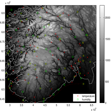
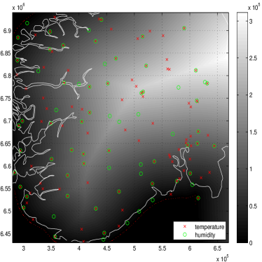
We build the analysis in this paper on a dataset containing observations for temperature and humidity on th of December each year from to year , i.e. for years. The temperature dataset contains daily mean temperature in Celsius degree and the humidity dataset contains the measured mixing ratio of humidity. The mixing ratio of humidity is defined as the mass of water vapor contained in a unit mass of dry air, and hence has a unit kg/kg. It is important to point it out that the observations are not necessarily at the same locations for all the years. Most of humidity observations are measured at a subset of locations of temperature. Two covariates are used in the model: elevation at the measurement location and the distance to the ocean. Figure 1 and Figure 1 give an overview of locations for temperature and humidity. The dotted line is the base line for calculating the distance to ocean and the solid line is the coast line of southern Norway. We can clearly note that the distance to ocean is not the same as the distance to the coast.
3 Background
3.1 Univariate GRFs in SPDE formulation
The main idea of the newly proposed approach by Lindgren et al. (2011) is to use an SPDE to construct GRFs for modelling spatial datasets. The SPDE used in this paper has the form
| (1) |
where is a parameter related to the variance of the random field , is a standard Gaussian white noise process, is a pseudo (fractional) differential operator and must be a non-negative integer. is the standard Laplacian with definition
Whittle (1954, 1963) has shown that the stationary solution to the SPDE (1) is a GRF with a Matérn covariance function. The Matérn covariance function has the form
| (2) |
where is the smoothness parameter, is the scaling parameter and is the modified Bessel function of second kind with order , denotes the Euclidean distance in and is the marginal variance. The Matérn covariance function is isotropic and it is widely used in spatial statistics (Stein, 1999; Diggle and Ribeiro Jr, 2006; Simpson et al., 2010; Lindgren et al., 2011; Bolin and Lindgren, 2011; Ingebrigtsen et al., 2013; Hu et al., 2012b, a). In this approach we use the finite element methods (FEMs) to solve the SPDE (1), and then apply the GMRF approximation to the solution in order to obtain computationally efficient inference. Bolin and Lindgren (2009) showed that the differences between the exact FEM representation and the GMRFs approximation are negligible. Since the smoothness parameter is poorly identifiable (Diggle and Ribeiro Jr, 2006; Lindgren et al., 2011), we fix for all our models to .
3.2 Multivariate GRFs in SPDE formulation
Hu et al. (2012b) have extended the approaches from Lindgren et al. (2011) to construct multivariate GRFs. This approach for constructing multivariate GRFs inherits both theoretical and computational advantages from the approach given by Lindgren et al. (2011) for univariate GRFs. The system of SPDEs for constructing a -dimensional multivariate GRF has the form
| (3) |
where are similar differential operators as given in Equation (1) with , are Gaussian noise processes which are independent but not necessarily identically distributed. It was shown by Hu et al. (2012b) that the solution to the system of SPDE (3) is a multivariate GRF. The parameters and are scaling parameters and smoothness parameters, respectively. are related to both the marginal variances of the fields and the cross covariances among the GRFs. Further, similarly as discussed by Lindgren et al. (2011), the precision matrix (inverse of the covariance matrix) for the multivariate GRF constructed from the system of SPDEs (3) satisfies the positive definite constraint automatically. Hu et al. (2012b) demonstrated that the link between the GMRFs and GRFs could be used, and hence we can construct models with GRFs but use GMRFs for computations. Since the precision matrix of the multivariate GMRF is sparse. Therefore numerical algorithms for sparse matrices can be applied for fast sampling and inference.
We follow Hu et al. (2012b, a) and use a triangular system of SPDEs
| (4) |
where are standard Gaussian white noise processes. This is a special case of the system of Equations (3) with and when . The advantage of a triangular systems of SPDEs is that this simplification makes both computations and interpretation easier.
With this setting we know that is a Matérn random field and is generally not a Matérn random field, but close to a Matérn random field (Hu et al., 2012b). This implies that the order of the random fields matters. Generally speaking, we need to choose the order of the random fields and , and this is usually done by a model selection test. Fit models with both orders and pick the one that minimizes some criterion, such as prediction error. Using the triangular system of SPDEs (4) for constructing a bivariate GRF, we have parameters to estimate from the system of SPDEs when we model the temperature and humidity jointly.
Hu et al. (2012b) showed that the sign of cross-correlation between and is only related to the product with a triangular system of SPDE. In the extreme case, if is zero, i.e., and are independent, then can only be positive value. Therefore we restrict to be positive and then the sign of the cross-correlation is decided by the sign of . When , and are positively correlated, and when , and are negatively correlated.
4 Models for temperature and humidity
We now set up three different Bayesian hierarchical models for temperature and humidity. The models have three levels, data model, process model and parameter models. We propose models differ in the dependency between temperature and humidity, i.e. they have different process models. To do inference we have available data that we denote , where is a location index, a year index and a field index. We have fields, , temperature and humidity, respectively. Further we have available data for years, . For each field and each year there are available observations at locations (see Table 1), , and the observations are not necessary measured at the same locations in each year.
Year temperature humidity
All models have the same data model. Given the truth the observed data is assumed to be Gaussian,
| (5) |
for . The variances and are interpreted to come from measurement uncertainty for temperature and humidity respectively. From knowledge about the measurement process we set the variances to and .
For each year the true temperature field and humidity field are modeled as a linear combination of explanatory variables and a spatial field. We use three explanatory variables, year as a factor, and elevation () and distance to ocean () as linear effects. The model can be written in vector form as:
| (6) |
| (7) |
where , , are design matrices and and are spatial fields for year for temperature and humidity, respectively. We now set up three models for the spatial fields which are all SPDE models as introduced in Section 3.1 and 3.2. Our first model assumes independent univariate SPDE models (UM) for and . The other two models allow for dependent fields, and are bivariate SPDE models. The triangular system of SPDEs in Section 3.2 gives us two modeling opportunities regarding the ordering: Modeling temperature as the first field (i.e. as a Matérn field), and humidity as the second field, which we denote BM-TH; or to model humidity as the first field and temperature as the second, BM-HT. Further, we assume that the fields for the different years are independent realizations of the same models, i.e. the parameters of the SPDE models do not change from year to year. The models for are summarized below:
- Independent univariate SPDE model (UM):
-
and are assumed independent and
(8) (9) - Bivariate SPDE model, TH (BM-TH):
-
We model temperature as the first field and humidity as the second. and are assumed to follow a bivariate SPDE-model with temperature as the first field in the formulation in Equation (4);
(10) where and .
- Bivariate SPDE model, HT (BM-HT):
-
We model humidity as the first field and temperature as the second. and are assumed to follow a bivariate SPDE-model with himidity as the first field in the formulation in Equation (4);
(11) where and .
The model formulations are completed by assigning priors to the parameters. All explanatory variable parameters (s) are given independent vague Gaussian priors; , while the SPDE parameters (s and s) are given independent log-Gaussian priors: and .
5 Evaluation
In this section we describe the scores and evaluation schemes used to compare the results of three different models set up in Section 4.
5.1 Scoring rules
In this paper the commonly used scoring rules mean absolute error (MAE), mean-square error (MSE) and the average of the continuous ranked probability score (CRPS) are chosen. Let denote the prediction for the observations for the observation in year for the th field, and then the MAE and MSE for the th field have the following definitions
The CRPS is also a commonly used scoring rule to evaluate the probabilistic forecasts, and it is the integral of the Brier scores for a continuous predictand at all possible threshold values (Hersbach, 2000; Gneiting et al., 2005). Let denote the predictive cumulative distribution function (CDF) and be the Heaviside function with value whenever and value 0 otherwise. Then the continuous ranked probability score is defined as
| (12) |
Gneiting et al. (2005) pointed out that if is the CDF of a Gaussian distribution, then a closed form of the continuous ranked probability score can be obtained, and this form is usually used in applications. The average of continuous ranked probability score, CRPS, then has the form
| (13) |
5.2 Validation scheme
To evaluate the predictive performance we use validation scheme where the data set is divided into a training set and a test set. The test sets consist of 20 locations that are chosen at random for each year among the locations that have observations for both temperature and humidity that year. The same test set is used for all three models and the following validation scheme has been chosen for comparing the results from different models.
Setting H
In this setting only predictive performance for humidity is evaluated. The model is fitted by using all
data but humidity observations for the test locations.
Setting T
In this setting only predictive performance for temperature is evaluated. The model is fitted by using all
data but temperature observations for the test locations.
Setting HT
In this setting both the predictive performance for temperature and humidity is evaluated. The model is fitted by using all
data but temperature and humidity observations for the test locations.
6 Results
In this seciton some empirical data analysis have been conducted in Section 6.1. Inference results of the parameters of the models set up in Section 4 are given in Section 6.2, while the results for predictive performance are given in Section 6.3.
6.1 Empirical data analysis
Since the numerical values of humidity observations are positive, they are preprocessed with the widely used Box-Cox family of transformations in order to transform them to be approximately Gaussian distributed (Box and Cox, 1964). The Box-Cox family of transformations has the form
| (14) |
The estimated value of for the Box-Cox transform is . The transformation function is a monotonic increase function and the transformed humidity is more reasonable to be modelled with Gaussian distribution. We use the original observations of temperature. Sakia (1992) and Diggle and Ribeiro Jr (2006) give more information about the Box-Cox transformation and other transformation methods.
The empirical variograms of both temperature and humidity have been calculated and fitted to theoretical variograms. In the theoretical variograms, we choose to fit with the Matérn model. This analysis suggest the smoothness parameters for both the fields with are reasonable, and hence fixing in our analysis is also reasonable.
6.2 Inference results of parameters
We follow Rue et al. (2009) and treat the coefficients for the covariates, and the yearly effects of temperature and humidity as parts of the latent field , i.e., , to achieve computational efficiency. This is due to the fact that there will be much fewer parameters during the optimization. Detailed setting of inference is given in Appendix B. It can be shown that
| (15) |
and
| (16) |
with , and given in Appendix B. From Equation (15) we can get the estimates for the yearly effects and for the coefficients of the covariates. For model BM-TH, we set as temperature and as humidity, and the estimates for the yearly effects are given in Table 2, with standard deviations given in brackets. Table 2 shows that the yearly effects are quite different. This explains the high temperature in but low temperature in . The estimates of the coefficients of the covariates are given in Table 3. We can notice that the two covariates give negative contribution to both fields. Similar results can be obtained when we change the order of the fields for the systems of SPDEs given in Equation (4), i.e., when we set the first field as humidity and the second field as temperature. These results agree with physical knowledge, and we summarize as follows: the higher elevation, the lower temperature; the higher elevation, the lower humidity; the longer distance to ocean, the lower temperature, and the longer distance to ocean, the lower humidity. We have standardized the elevation and distance to ocean by divide them with and , respectively, and hence the inference is more stable.
Model Parameter BM () () () () () () () () () () UM () () () () () () () () () ()
Model Parameter Estimate Std. dev. BM UM
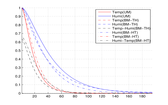
The posterior mean estimates estimates and the posterior standard deviations are given for the bivariate models in Table 4. We notice that temperature and humidity are positively correlated since and for the two models. The results for all three models, i.e., UM, BT-TH and BT-HT, are given in Figure 2.
From the results shown in Table 5 and 2 we notice that the correlation range differ between models. We further notice that the correlation ranges of humidity and temperature from UM are the longest and shortest, respectively comparing to the results from BM-TH and BM-HT. The cross-correlations between temperature and humidity at the same location are and for BM-TH and BM-HT, respectively. From these results we conclude that the cross-correlation between temperature and humidity are relatively high and indeed needed to be considered.
BM-TH BM-HT UM () () () () () () () () () () () () () () () ()
BM-TH km km km BM-HT km km km UM km km
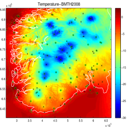
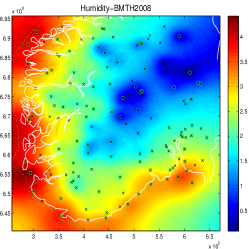
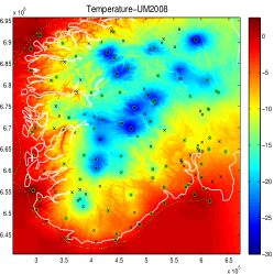
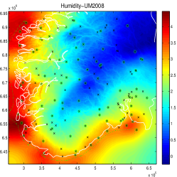
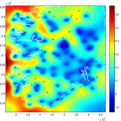
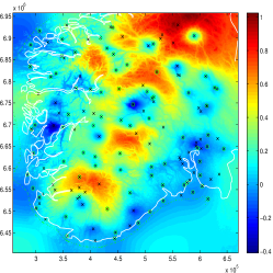
With the estimates given in Section 6.2, we can reconstruct temperature and humidity over the northern Norway with km by km resolution. Figure 3 shows the reconstructed temperature and humidity in for bivariate model (BM-TH) (a) - (b) and for univariate model (c) - (d). The fields are reconstructed by first estimating the relevant parameters with lower resolution model, and then use the posterior modes for the parameters and the covariates for the km by km resolution model. The differences between these two models are shown in Figure 3 and in Figure 3. From these two figures we find that the differences at the locations where the observations are available are small, while the differences are larger when it is further away from the observations. With the bivariate model we use the variance-covariance structure to borrow information between humidity and temperature. From Figure 3 we can also notice that humidity is less influenced by elevation in the bivariate model than the univariate mode since the bivariate model borrows some information from temperature and we have more temperature observations in the dataset. It is further illustrated with the predictive performance in Section 6.3.
6.3 Predictive performance
In this section the predictive performance for the bivariate models (BM-TH and BM-HT) and univariate model (UM) are compared using the scores and validation scheme from Sections 5.1 and 5.2.
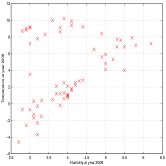
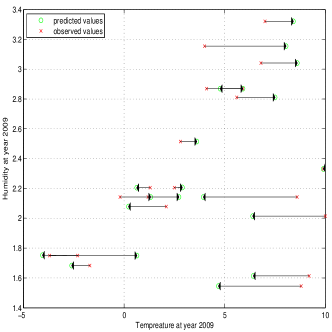
From Figure 4 we can see that there are some “outliers” in the temperature observations in year : there are some locations with very high temperature but rather low humidity. This will cause poor predictive performance. We therefore now first discuss predictions based on results excluding 2009 from the test dataset, and then come back to later. Figure 4 illustrates the dataset where both temperature and humidity observations are available and Figure 4 shows the test dataset.
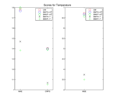
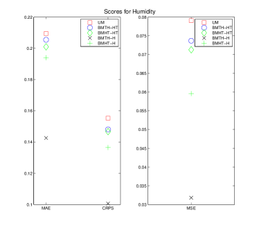
The scores for predictions are given in Figure 5, and Figure 5 and Figure 5 illustrate the predictive scores for temperature and humidity, respectively. In these figures, “BMTH” and “BMHT” denote the bivariate model with temperature as the first field and humidity as the second field, and with humidity as the first field and first as the second field, respectively. “-T”, “-H” and “-HT” denote the validation settings. From the results we can notice that the bivariate model with Settings “H” and “T” perform better than the univariate model for all scores. We can also notice that the bivariate model with Settings “H” and “T” perform better than the bivariate model with Setting “HT”. In addition, we can notice that the bivariate model with Setting “HT” performs better than the univariate models. In other words, when observations from one field are available (validation setting “H” and setting “T”), the bivariate models perform better than the univariate model. Further, if neither temperature nor humidity observations are available at the test locations (validation setting “HT”), the bivariate models perform better than the univariate model, but not as good as when observations of the other quantity is available at the test locations.
From Figure 5 we further notice that the order of the fields matters for the predictive performance. It shows that we get better results when we set the corresponding field as the second field, especially for validation settings “H” and “T”. For instance, if we are interested in predicting humidity, the result is better when it is set as the second field, especially when temperature observation at the test locations are available. However, the bivariate models perform better than the univariate model regardless of the order of fields.
Regarding year , the bivariate models perform worse than the univariate model, especially when the other quantity is available at the test location , i.e., the CRPS values temperature with ’UM’, ’BMTH’ with validation setting ’HT’, and ’BMTH’ with validation setting ’H’ are and , respectively, because the ’borrowed’ information is wrong in the bivariate models. This result is useful since in this case it can be used as an indicator of outliers in our dataset which might need special treatment. We notice in Figure 4 that the bivariate model ’BMTH’ with validation setting ’H’ tries to drag the outliers back to follow the positive correlation.
7 Discussion and Conclusion
In this paper we have set up, fitted and evaluated models for temperature and humidity in Southern Norway based on the observations on th of December from to using elevation and distance to ocean as explanatory variables. Three different models are compared in this paper: two bivariate models for modelling temperature and humidity jointly, and one univariate model for modelling them independently. To set up bivariate models the system of SPDEs approach proposed by Hu et al. (2012b) is used, while the corresponding univariate approach is chosen for univariate models. For all models the parameters for the explanatory variables agree with physical knowledge. Further, there are spatial dependence both for humidity and temperature, and the bivariate models shows also positive spatial cross-correlation.
To compare predictive performance between the three models, three different validation settings are used. We conclude that using a bivariate GRF to model temperature and humidity jointly is superior to model them independently using univariate GRFs, both in term of prediction accuracy (has lower RMSE), and in term of quantifying prediction uncertainty (has lower mean CRPS). Using a bivariate model is especially useful for predicting humidity, as it has a sparser network than temperature. For locations at or close to a temperature observation the bivariate model is able to utilize this information when predicting humidity.
The results also illustrate that the order of fields is relevant from the prediction point of view when we use a triangular system of SPDEs for constructing a bivariate field. From an applied point of view, the results from both orders are satisfiable, and we do not need to consider both if the computational resources or time is limited. We have found that if one of the quantities is our prime interest, this should be the second field which is given a model that is a mixture of Matérn models. From a modeling point of view it is interesting that it seems to be beneficial to use a mixture of Matérn models, and this model class is an interesting topic for future research.
From our results we have learned that the bivariate models do not always perform better than the univariate model. In year there were a group of observations that did not follow the general positive dependency between temperature and humidity, but seemed to be independent. One way to tackle this could be to extend the bivariate model to allow for a spatial varying dependency. To set up such a model has to be done carefully to ensure positive definite covariance functions and to keep the computational efficiency, and this is outside the scope of this paper.
There might be some other explanatory variables, such as wind speed and solar radiation, which should be included in the model. Further, there is, for a given pressure and temperature an upper limit of humidity (Barry and Chorley, 2010). This physical limitation is not included in our model. All these might improve the predictive performance of our model. On the other hand, the purpose of our modeling is to provide input to a deterministic physically based model for precipitation. This model would convert the nonphysically high humidity to precipitation, which might give good predictions for precipitation. From an applied point of view, we find incorporating our results with a physical model for precipitation and evaluate the differences between our models with respect to precipitation predictions is the most interesting direction for further work.
Appendix A. Gaussian Markov random fields
A random vector is a Gaussian random field with mean and precision matrix () if and only if its density is
| (17) |
where denotes for . denotes that it is positive definite. Gaussian Markov random fields are the main tool for achieving computational efficiency with models built by the SPDE approach. A Gaussian Markov random fields is a GRF with Markov property
| (18) |
and hence the precision matrix for a GMRF is usually sparse. Therefore, numerical algorithms for sparse matrices can be applied when doing computations. Rue and Held (2005) gives a more detailed discussion on the theories for GMRFs. A condensed discussion about GMRFs can also be found in Gelfand et al. (2010, Chapter ).
Appendix B. Inference
Since the coefficient parameters for the covariates can be modelled with Gaussian distributions, we can treat the coefficients as part of the latent field together the spatial process and model them jointly instead of treating the coefficient parameters as hyper-parameters. The hyper-parameters then only contains the parameters from the systems of SPDEs (4), for bivariate model and for univariate model, since we fix the values of for both the models. The latent field in this case is , where T denotes the transpose of a vector or a matrix. This can speed up the optimization considerably since there are much fewer parameters in the numerical optimization. This is the commonly used setting in Rue et al. (2009).
Let denote the precision matrix for the random fields constructed by the system of SPDEs (4) for the bivariate GRFs or the precision matrix for the univariate random fields with SPDE (1) with hyper-parameters . With the univariate model we construct the precision matrix as a block diagonal precision matrix, then inference for this two univariate random fields can be done simultaneously. In this case we can use the same program for the bivariate model, and the univariate model has only one more constraint . Hu et al. (2012b) have shown that from the well known Bayesian formula
| (19) |
we can derive the posterior distribution
| (20) |
with , , and . is a sparse matrix which links the sparse observations of temperature and humidity to our bivariate GRF or univariate GRFs. is the design matrix.
References
- Apanasovich and Genton (2010) Tatiyana V Apanasovich and Marc G Genton. Cross-covariance functions for multivariate random fields based on latent dimensions. Biometrika, 97(1):15–30, 2010.
- Apanasovich et al. (2012) T.V. Apanasovich, M.G. Genton, and Y. Sun. A valid matérn class of cross-covariance functions for multivariate random fields with any number of components. Journal of the American Statistical Association, 107(497):180–193, 2012.
- Barry and Chorley (2010) Roger G Barry and Richard J Chorley. Atmosphere, weather and climate. Routledge, 9th edition, 2010.
- Bolin and Lindgren (2009) D. Bolin and F. Lindgren. Wavelet markov models as efficient alternatives to tapering and convolution fields. Technical report, Mathematical Statistics, Centre for Mathematical Sciences, Faculty of Engineering, Lund University, 2009.
- Bolin and Lindgren (2011) D. Bolin and F. Lindgren. Spatial models generated by nested stochastic partial differential equations, with an application to global ozone mapping. The Annals of Applied Statistics, 5(1):523–550, 2011.
- Box and Cox (1964) G.E.P. Box and D.R. Cox. An analysis of transformations. Journal of the Royal Statistical Society. Series B (Methodological), pages 211–252, 1964.
- Brown et al. (1994) P.J. Brown, N.D. Le, and J.V. Zidek. Multivariate spatial interpolation and exposure to air pollutants. Canadian Journal of Statistics, 22(4):489–509, 1994.
- Courtier et al. (1998) P. Courtier, E. Andersson, W. Heckley, D. Vasiljevic, M. Hamrud, A. Hollingsworth, F. Rabier, M. Fisher, and J. Pailleux. The ecmwf implementation of three-dimensional variational assimilation (3d-var). i: Formulation. Quarterly Journal of the Royal Meteorological Society, 124(550):1783–1807, 1998.
- Cressie and Wikle (2011) N. Cressie and C.K. Wikle. Statistics for spatio-temporal data, volume 465. Wiley, 2011.
- Cressie (1993) N.A.C. Cressie. Statistics for spatial data, volume 298. Wiley-Interscience, 1993.
- Diggle and Ribeiro Jr (2006) P.J. Diggle and P.J. Ribeiro Jr. Model-based Geostatistics. Springer, 2006.
- Fuglstad et al. (2014) G.A. Fuglstad, F. Lindgren, D.P. Simpson, and H. Rue. Exploring a new class of non-stationary spatial gaussian random fields with varying local anisotropy. Statistica Sinica, page to appear, 2014.
- Gel et al. (2004) Y. Gel, A.E. Raftery, and T. Gneiting. Calibrated probabilistic mesoscale weather field forecasting. Journal of the American Statistical Association, 99(467):575–583, 2004.
- Gelfand et al. (2004) A.E. Gelfand, A.M. Schmidt, S. Banerjee, and CF Sirmans. Nonstationary multivariate process modeling through spatially varying coregionalization. Test, 13(2):263–312, 2004.
- Gelfand et al. (2010) A.E. Gelfand, P.J. Diggle, M. Fuentes, and P. Guttorp. Handbook of spatial statistics. CRC Press, 2010.
- Gneiting et al. (2005) T. Gneiting, A.E. Raftery, A.H. Westveld III, and T. Goldman. Calibrated probabilistic forecasting using ensemble model output statistics and minimum crps estimation. Monthly Weather Review, 133(5):1098–1118, 2005.
- Gneiting et al. (2010) T. Gneiting, W. Kleiber, and M. Schlather. Matérn Cross-Covariance Functions for Multivariate Random Fields. Journal of the American Statistical Association, 105(491):1167–1177, 2010. ISSN 0162-1459.
- Goulard and Voltz (1992) M. Goulard and M. Voltz. Linear coregionalization model: tools for estimation and choice of cross-variogram matrix. Mathematical Geology, 24(3):269–286, 1992. ISSN 0882-8121.
- Hersbach (2000) H. Hersbach. Decomposition of the continuous ranked probability score for ensemble prediction systems. Weather and Forecasting, 15(5):559–570, 2000.
- Hu et al. (2012a) X. Hu, F. Lindgren, D.P. Simpson, and H. Rue. Multivariate gaussian random fields with oscillating covariance functions using systems of stochastic partial differential equations. statistical report, Norwegian University of Science and Technology, 2012a.
- Hu et al. (2012b) X. Hu, D.P. Simpson, F. Lindgren, and H. Rue. Multivariate gaussian random fields using systems of stochastic partial differential equations. statistical report, Norwegian University of Science and Technology, 2012b.
- Ingebrigtsen et al. (2013) R. Ingebrigtsen, F. Lindgren, and I. Steinsland. Using stochastic partial differential equation models for spatial reconstruction of annual precipitation. submitted, 2013.
- Kleiber and Nychka (2012) William Kleiber and Douglas Nychka. Nonstationary modeling for multivariate spatial processes. Journal of Multivariate Analysis, 112:76–91, 2012.
- Konigsberg and Ousley (2009) L.W. Konigsberg and S.D. Ousley. Multivariate quantitative genetics of anthropometric traits from the boas data. Human biology, 81(5/6):579–594, 2009.
- Li and Zhang (2011) Bo Li and Hao Zhang. An approach to modeling asymmetric multivariate spatial covariance structures. Journal of Multivariate Analysis, 102(10):1445–1453, 2011.
- Lindgren et al. (2011) F. Lindgren, H. Rue, and J. Lindström. An explicit link between gaussian fields and gaussian markov random fields: the stochastic partial differential equation approach. Journal of the Royal Statistical Society: Series B (Statistical Methodology), 73(4):423–498, 2011.
- Mcguigan (2006) K. Mcguigan. Studying phenotypic evolution using multivariate quantitative genetics. Molecular ecology, 15(4):883–896, 2006.
- Reich and Fuentes (2007) B.J. Reich and M. Fuentes. A multivariate semiparametric bayesian spatial modeling framework for hurricane surface wind fields. The Annals of Applied Statistics, 1(1):249–264, 2007.
- Ribeiro Jr and Diggle (2006) P.J. Ribeiro Jr and P.J. Diggle. MODEL BASED GEOSTATISTICS. Springer Series in Statistics. Springer, 2006.
- Rue and Held (2005) H. Rue and L. Held. Gaussian Markov random fields: theory and applications. Chapman & Hall, 2005. ISBN 1584884320.
- Rue et al. (2009) H. Rue, S. Martino, and N. Chopin. Approximate Bayesian inference for latent Gaussian models by using integrated nested Laplace approximations. Journal of the Royal Statistical Society: Series B (Statistical Methodology), 71(2):319–392, 2009. ISSN 1467-9868.
- Sain and Cressie (2007) S.R. Sain and N. Cressie. A spatial model for multivariate lattice data. Journal of Econometrics, 140(1):226–259, 2007.
- Sakia (1992) RM Sakia. The box-cox transformation technique: a review. The statistician, pages 169–178, 1992.
- Schmidt and Gelfand (2003) A.M. Schmidt and A.E. Gelfand. A bayesian coregionalization approach for multivariate pollutant data. Journal of Geophysical Research, 108(D24):8783, 2003.
- Simpson et al. (2010) D. Simpson, F. Lindgren, and H. Rue. In order to make spatial statistics computationally feasible, we need to forget about the covariance function. Environmetrics, 2010.
- Stein (1999) M.L. Stein. Interpolation of Spatial Data: some theory for kriging. Springer Verlag, 1999. ISBN 0387986294.
- Wackernagel (2003) H. Wackernagel. Multivariate geostatistics: an introduction with applications. Springer Verlag, 2003. ISBN 3540441425.
- Whittle (1954) P. Whittle. On stationary processes in the plane. Biometrika, 41(3-4):434–449, 1954. ISSN 0006-3444.
- Whittle (1963) P. Whittle. Stochastic processes in several dimensions. Bull. Int. Statist. Inst., 40:974–994, 1963.