Multivariate Gaussian Random Fields with Oscillating Covariance Functions using Systems of Stochastic Partial Differential Equations
Abstract
In this paper we propose a new approach for constructing multivariate Gaussian random fields (GRFs) with oscillating covariance functions through systems of stochastic partial differential equations (SPDEs). We discuss how to build systems of SPDEs that introduces oscillation characteristics in the covariance functions of the multivariate GRFs. By choosing different parametrization of the equations, some GRFs can be made with oscillating covariance functions but other fields can have Matérn covariance functions or close to Matérn covariance functions. The multivariate GRFs constructed by solving the systems of SPDEs automatically fulfill the hard requirement of nonnegative definiteness for the covariance functions. The approximate weak solutions to the systems of SPDEs are used to represent the multivariate GRFs by multivariate Gaussian Markov random fields (GMRFs). Since the multivariate GMRFs have sparse precision matrices (inverse of the covariance matrices), numerical algorithms for sparse matrices can be applied to the precision matrices for sampling and inference. Thus from a computational point of view, the big-n problem can be partially solved with these types of models. Another advantage of the method is that the oscillation in the covariance function can be controlled directly by the parameters in the system of SPDEs. We show how to use this proposed approach with simulated data and real data examples.
Keywords: Multivariate Gaussian random fields, Oscillating covariance functions, Multivariate Gaussian Markov random fields, Sparse matrix, Stochastic partial differential equations
1 Introduction
Statistics for spatial data appeared from hundreds of years ago, but spatial models for this type of data appeared much later (Cressie, 1993). The spatial models have been widely used to model the spatial data in many areas. Gaussian random fields (GRFs) are some of the most commonly used models in spatial statistics. Since the normalizing constant can be computed explicitly, the GRFs are convenient to be used in many applications, such as geo-statistical data, environmental and atmospheric data, longitudinal and survival data (Cressie, 1993; Stein, 1999; Rue and Held, 2005; Gelfand et al., 2010). GRFs also have other good properties, such as the fact that a GRF can be explicitly specified through a mean and a covariance function . Let the coordinates members of . If is Gaussian for every selection of points for every , then we call a continuously indexed GRF. The covariance matrix of a collection is given by . However, there is a hard nonnegative definite requirement that must be fulfilled for the function . This is one of the main concerns when we build models with GRFs using covariance function based approaches.
A widely used class of covariance functions is the Matérn family which was introduced by Matérn (Matérn, 1986). This family of covariance functions captures the most common form of the empirical behavior of stationary covariance functions, namely that the correlation between the locations and should decrease when the Euclidean distance increases (Diggle and Ribeiro Jr, 2006). This family of covariance functions is isotropic and usually written as , where is the Matérn correlation function between the spatial locations . The Matérn correlation function is a two-parameter family with the form
| (1) |
where is the marginal variance, is the modified Bessel function of second kind and is the scaling parameter. The order is a smoothness parameter and must be positive. The smoothness parameter is of critical concern in spatial statistics since it defines the differentiability of the sample paths and the Hausdorff dimension (Goff and Jordan, 1988; Handcock and Stein, 1993; Gneiting et al., 2010). It is known that the smoothness parameter is poorly identifiable from the data and hence it is usually fixed (Diggle and Ribeiro Jr, 2006; Lindgren et al., 2011; Hu et al., 2012a). The Matérn family contains the commonly used models with exponential covariance function . The Matérn covariance function is the key factor in the explicit link between the GRFs and GMRFs through the stochastic partial differential equations (SPDEs) discussed by Lindgren et al. (2011). Gneiting et al. (2010) presented one direct approach for constructing the multivariate GRFs by using matrix-valued covariance functions, and all components in the matrix-valued covariance function are Matérn covariance functions. Hu et al. (2012a) discussed the important role of Matérn covariance function for constructing stationary and isotropic multivariate GRFs with systems of SPDEs.
In spatial statistics oscillating models usually deal with ocean waves, and we usually work entirely with their spectra only rarely with covariance functions (Lindgren, 2010). For time series there are plenty of applications with oscillating models in discrete time since the -order auto-regressive (AR()) processes can result in oscillating models (Wei, 2006). However, it is less common for continuous time models. Lindgren et al. (2011) have discussed an approach for constructing univariate GRFs with oscillating covariance functions. In their approach they have chosen a coupled system of SPDEs to construct two independent random fields with the same precision matrix. Their discussion was focused on the case . Since it is important for our approach for constructing multivariate GRFs with oscillating covariance functions, we give an overview of their approach in Section 3.1.
In this paper we focus on the methodology for constructing multivariate GRFs with oscillating covariance functions through systems of SPDEs. This work is an extension of the discussion given by Lindgren et al. (2011) for the univariate case. It is also an extension of the approach discussed by Hu et al. (2012a) to construct larger class of useful models. In our approach the GRFs are constructed by solving systems of stochastic partial differential equations. One of the main advantages of this approach is that we do not need to consider the notorious nonnegative definite requirement for the covariance functions. This requirement is fulfilled automatically because we are working on the processes directly. During the computational stage the GRFs are represented by the Gaussian Markov random fields (GMRFs) by GMRF approximations. A GMRF is a discretely indexed GRF with some Markov property. The full conditionals of a GMRF depend only on a set of neighbors of each site . Denote the neighbors of the node by . The Markov property implies that if and only if , where denotes the precision matrix of the GMRF. Consistency requirement implies that if , then . The precision matrix for the GMRF is sparse which enables us to use numerical algorithms for sparse matrices. Thus the big-n problem (Banerjee et al., 2004) can be partially solved in our case with these types of models. We refer to Rue et al. (2009, Section 2.1) for a condensed overview of the theory of GMRFs. Detailed discussions about GMRFs are given in Rue and Held (2005, Chapter 2).
2 State-of-the-art and preliminaries
We review the state-of-the-art research on GRFs with SPDE approach in Section 2.1 and the methodologies for constructing multivariate GRFs in Section 2.2. The GMRF approximation for representing a GRF with a GMRF is introduced in Section 2.3 since it is crucial for computations.
2.1 GRFs through the SPDE approach
As mentioned in Section 1, Lindgren et al. (2011) proposed a novel approach for constructing GRFs by using the SPDE
| (2) |
where is a pseudo-differential operator, is the scaling parameter, is related to the smoothness parameters and . is the Laplacian with definition
A range parameter connects the scaling parameter and the smoothness parameter . The simple and empirically derived relationship is commonly used (Lindgren et al., 2011; Hu et al., 2012a). It corresponds to correlation near at distance , with parameters and . is the innovation process which is a standard spatial Gaussian white noise. The most important result given by Whittle (1954, 1963), and used by Lindgren et al. (2011) extensively, is that the solution to SPDE (2) is a GRF with the Matérn covariance function given in Equation (1). We follow the terminology used by Lindgren et al. (2011) and call GRFs with Matérn covariance functions Matérn random fields. Lindgren et al. (2011) commented that their approach can be extended in many directions.
Fuglstad (2011) has extended the SPDE approach to include a diffusion matrix in Equation (2) which provides a way of controlling the covariance structures of the GRF. Using the diffusion matrix in SPDE (2), it is not only possible to construct homogeneous isotropic fields, but also anisotropic fields. Fuglstad (2011) showed that it is possible to construct inhomogeneous fields. The SPDE discussed by Fuglstad (2011) has the form
| (3) |
where is a matrix-valued function, is the gradient operator and is a standard spatial Gaussian white noise process. The main contribution of Fuglstad (2011) is that he introduced the matrix to (2) to control the structure of covariance matrix. However, he focused on discussing the univariate GRFs with .
Bolin and Lindgren (2011) discussed how to use nested SPDEs to construct stationary and non-stationary GRFs. The equation chosen by Bolin and Lindgren (2011) has the form
| (4) |
for some linear differential operators and . is a standard spatial Gaussian white noise process. The SPDE (4) may not exist in the common sense since the operator may contain some differentiation of the noise process . In this case SPDE (4) can then be interpreted as the following nested system of SPDEs
| (5) |
when and are commutative operators. As pointed out by Bolin and Lindgren (2011) this interpretation not only avoids the apparent problem with the differentiation of the Gaussian white noise process, but also gives an interpretation of the consequence of the additional differential operator . The random field is obtained by applying to the solution of (4) with .
Fuglstad (2010) discussed the approximated solutions to a SPDE for constructing space-time GMRFs. The equation discussed by him has the form
| (6) |
where, , is a constant and is Gaussian space-time white noise. Fuglstad (2010) only discussed and argued that this equation has real physical meaning since the prototype of (6) is the stochastic heat equation
| (7) |
The heat equation relates the change of the size in time to the spatial divergences of the flux and the source term . Fuglstad (2010) chose a finite volume method for solving Equation (6), and claimed that the finite volume method gave the correct distribution of the total energy of the solution to SPDE (6).
Lindgren et al. (2011) discussed the methodology for constructing non-stationary GRFs and non-separable space-time models. They claimed that if the parameters and depend on the coordinate , then we can construct a non-stationary GRF. The SPDE then has the form
| (8) |
The non-separable space-time models have interaction between space and time in the covariance structure. In general it is difficult to construct this kind of model through a covariance function based approach. However, the SPDE approach can be used. One of the non-separable SPDEs which can result in this kind of model is
| (9) |
where is a transport vector, is a positive definite diffusion matrix and is a stochastic space-time noise process. We refer to Lindgren et al. (2011, Section ) for detailed discussion on this topic.
2.2 Multivariate GRFs
A multivariate GRF with components , , is a collection of continuously indexed multivariate normal random vectors such that
where is the mean of the random field and is the covariance matrix. Assume, at the current stage, that the process is second-order stationary with mean zero. One approach for constructing stationary and isotropic multivariate GRFs using covariance-based models was proposed by Gneiting et al. (2010). The covariance function in their approach is given by
| (14) |
where are the marginal covariance functions and are the cross-covariance functions. give information about the covariance structures within the fields . describes the covariance structure between fields and . are the co-located correlation coefficients. are the marginal variances, and and are the corresponding standard deviations. They satisfy the relationships throughout this paper . The main difficulty in constructing useful multivariate models using this kind of approach is the nonnegative definiteness requirement for the covariance functions. Gneiting et al. (2010) proposed a way to specify valid parametric models through the covariance functions given in Equation (14) directly. Several theorems were presented in order to ensure the matrix-valued covariance function to be symmetric and nonnegative definite.
Hu et al. (2012a) proposed to use a system of SPDEs to construct a multivariate GRF. They claimed that the notorious requirement nonnegative definiteness for the covariance function is automatically fulfilled with their approach. Hu et al. (2012a) also discussed the link between the system of SPDEs approach and the covariance function based approach discussed by Gneiting et al. (2010). The system of SPDEs which has been used for constructing the multivariate GRFs by Hu et al. (2012a) is
| (15) |
where are differential operators with , and are scaling parameters and smoothness parameters. are independent but not necessarily identically distributed noise processes, and are the parameters related to the marginal variances of the fields and the cross-covariances between the fields. Hu et al. (2012a) pointed out that the GMRF approximation can be applied to the GRFs. Hence they can use computationally efficient GMRFs for sampling and inference. However, the constructed GRFs are always stationary and isotropic, and the covariance functions are not oscillating.
2.3 GMRFs approximation to GRFs
Generally speaking, GRFs are commonly used in statistical modelling because of their good theoretical properties. However, the GRFs have a bottle-neck on the computational side. The computational cost for factorizing a dense covariance matrix with dimension is . Even though the computational power is at an all time high, it seems that in many situations it is infeasible to do the computations in reasonable time. Banerjee et al. (2004, Appendix A.5) informally call this situation “the big problem”.
There are many different approaches trying to avoid or overcome “the big problem”, such as covariance tapering (Furrer et al., 2006; Zhang and Du, 2008; Kaufman et al., 2008; Shaby and Ruppert, 2012), likelihood approximations (Vecchia, 1988; Stein et al., 2004), and fixed rank kriging and fixed rank filtering (Cressie and Johannesson, 2008; Cressie et al., 2010) . The approach which has been chosen in this paper is based on the GMRF approximation to GRFs. The sparsity of the precision matrix enables the numerical algorithms for sparse matrix for fast inference with large datasets (Rue, 2001; Rue and Held, 2005; Lindgren et al., 2011). The general cost for factorizing the sparse matrix is , and in one dimension, two dimensions and three dimensions, respectively (Rue and Held, 2005). Hartman and Hössjer (2008) proposed to use the GMRFs for GRFs for spatial prediction with Kriging, due to the pleasant computational properties of GMRFs.
In this paper we only give an overview of GMRF approximation to univariate GRF and refer to Hu et al. (2012a, Section ) for detailed discussion on GMRF approximation to multivariate GRF. In order to find a GMRF approximation of a GRF on a triangulated lattice, we at first need to find the stochastic weak formulation of SPDE (2) (Kloeden and Platen, 1999). In this paper we use Delaunay triangulation. We refer to Hjelle and Dæhlen (2006) for more information about triangulations. Denote the inner product of functions and as
| (16) |
where the integration is within the region of interest. The stochastic weak solution of SPDE (2) is found by requiring
| (17) |
where is the number of test functions and “” denotes equality in distribution.
Then we need to find the finite element representation of the solution to the SPDE. The finite element representation of the solution is
| (18) |
with basis functions and Gaussian distributed weights . is the number of vertexes in the triangulation. We refer to Zienkiewicz et al. (2005) and Brenner and Scott (2008) for more information and theoretical background of finite element methods. The approach given by Lindgren et al. (2011) for choosing the basis functions is used in this paper. With we choose each basis function to be piecewise linear on each triangle with at vertex and at other vertexes. This choice of basis functions means that the local interpolation on a triangle is linear. Lindgren et al. (2011) pointed out that other methods, such as kernel method, are useful in theory but not necessary in practice. When the least squares approximation is chosen, . When the Galerkin solution is chosen, . When the recursive Galerkin formulation is used. We refer to Lindgren et al. (2011, Section ) for more information about the recursive Galerkin formation.
2.4 Outline of the paper
The structure of the rest of the paper is organized as follows. Section 3 gives the detailed discussion on how to construct multivariate GRFs with oscillating covariance functions through the systems of SPDEs approach. Examples with simulated data and real data are given in Section 4. Discussion and future work in Section 5 ends this paper.
3 Model formulation
GRFs with oscillating covariance functions can be used in many situations, for example, for modelling global pressure (Lindgren et al., 2011) and ocean waves (Lindgren, 2010). First, an overview for constructing the univariate GRFs with oscillating covariance function is given since it is needed for constructing multivariate GRFs with oscillating covariance functions. Next, we introduce a general approach for constructing the multivariate GRFs with oscillating covariance functions. Then explicit approach for constructing the bivariate GRFs is discussed. At last we discuss the procedure for sampling the multivariate GRFs with oscillating covariance functions.
3.1 Univariate GRFs with oscillating covariance functions
Lindgren et al. (2011, Section ) discussed how to construct an univariate GRF with oscillating covariance function using a SPDE with complex number. For the case the SPDE has the form
| (19) |
where is the oscillation parameter, , and . The innovation processes and are independent standard Gaussian white noise processes. Lindgren et al. (2011) pointed out that the real and imaginary parts, and , of the stationary solution are independent with identical spectrum densities
| (20) |
With this approach the common isotropic stationary Matérn random fields can be obtained by setting . We can notice that generates intrinsic stationary random fields. We refer to Rue and Held (2005, Chapter 3) for more information on the intrinsic random fields. When , the constructed GRFs have covariance functions with oscillation. The oscillation is increasing with larger value of . The closed form of the precision matrix for the stationary GRFs with oscillation can be obtained from (20),
| (21) |
The matrices and in Equation (21) are defined through
| (22) |
with basis functions . We use , instead of in order to make the precision matrix sparse. This setting yields a Markov approximation to the FEM solution. Bolin and Lindgren (2009) studied the effects of the Markov approximation and claimed that the difference between the Markov approximation and exact FEM representation is negligible.
Lindgren et al. (2011) pointed out that this complex-valued version of SPDE (19) can be rewritten as a special case of the coupled systems of SPDEs
| (23) |
where and . The random fields and from Equation (23) have the same precision matrix given in Equation (21). Lindgren et al. (2011) commented that it is surprising that these two fields from the coupled system of SPDEs (23) are always independent regardless of the choices of parameters. Additionally, the univariate GRFs with oscillating covariance functions from Equation (19) are always isotropic. However, it is possible to construct non-isotropic GRFs by slightly modifying the coupled system of SPDEs (23). We are not going to discuss this issue here and we focus only on the isotropic GRFs. We refer to Lindgren et al. (2011, Appendix C.4) for more information about the oscillating and non-isotropic cases.
3.2 Multivariate GRFs with oscillating covariance functions
The multivariate GRFs with oscillating covariance functions, in this paper, all have the assumption that the mean is zero, i.e., . Hu et al. (2012a) proposed to construct the multivariate GRFs using the system of SPDEs given in (15). In their approach the multivariate GRFs are always isotropic and stationary. The covariance functions cannot be oscillating. They argued that, under some conditions, it is possible to construct the multivariate GRFs with Matérn covariance functions as discussed by Gneiting et al. (2010). In this section we are going to discuss how to construct multivariate GRFs where some components of the random fields have oscillating covariance functions. The main idea is to replace the noise processes by noise processes with oscillating covariance functions. With this approach the systems of SPDEs have the same form as given in (15), but the noise processes are different. Even though the system of SPDEs in (15) is theoretically general, we recommend to use the triangular system of SPDEs in applications. The triangular system of SPDEs is
| (24) |
where are differential operators as defined in (15), and are noise processes where some of them have oscillating covariance functions. We recommend to use as fewer noise processes with oscillating covariance functions as possible. This system has many advantages, such as interpretation of the properties of the fields. For example, we know which components of the random field must have non-oscillating covariance functions and have oscillating covariance functions. However, there are some components of the random field which might have oscillating covariance functions. We divide the random fields into three categories , and , where denotes the random fields with non-oscillating covariance functions, denotes the random fields with oscillating covariance functions and denotes the random fields with covariance functions which might be oscillating. Assume that only is the noise process with oscillating covariance function and other noise processes are noise processes with non-oscillating covariance functions, and then we can obtain the following results.
-
•
If only the covariance function for the noise process is oscillating, the covariances functions for all the random fields are non-oscillating, ;
-
•
If only the covariance function for the noise process is oscillating, the random field has an oscillating covariance function,
-
•
If only the covariance function for the noise process is oscillating, the random fields belong to , which means that the covariance functions for these random fields might be oscillating.
This result is rather intuitive since we can obtain it by checking the system of SPDEs (24) directly. However, these results are important in the real-world application since it gives information for how to build models in a reasonable way. For instance, we can get information about how to choose the order of the random fields.
3.3 Bivariate GRFs with oscillating covariance functions
The methodology for constructing non-oscillating and isotropic bivariate GRFs explicitly has been studied by Gneiting et al. (2010) and Hu et al. (2012a). In this section we discuss the approach for constructing bivariate GRFs explicitly with oscillating covariance functions using systems of SPDEs. We start the investigation with random fields constructed by the full system of SPDEs
| (25) |
where and are the same as in (15), and are noise processes which can have oscillating covariance functions. By changing the properties of the noise processes we can construct more interesting random fields. Use the matrix notion and define the operator matrix as
| (26) |
and let , where H denotes the Hermitian transpose of a vector or a matrix. is defined as the collection of parameters for . The system of equations (25) can then be written in a compact matrix form as
| (27) |
where . With (27) we can obtain the power spectrum by
| (28) |
where denotes the inverse of the complex conjugate of the matrix. is the Fourier transform of , , and is the Fourier transform of the operator matrix ,
| (29) |
is the power spectrum matrix for the independent noise processes
| (30) |
where is the frequency. Since the noise processes are mutually independent, the power spectrum matrix of noise processes is a diagonal matrix. Using Equation (28) - Equation (29), the elements in the power spectrum matrix of the bivariate fields from the full system of SPDEs in (25) can be obtained,
| (31) |
Define poles and zeros as the roots of the denominators and numerators of the power spectrum elements , respectively. From (31), we can see that the poles of the power spectrum, in general, are the same for both the fields, but zeros of the power spectrum will be different. It gives us a possibility to construct bivariate GRFs with oscillating covariance functions by carefully re-parametrization of system of SPDEs (25). However, we will not discuss this approach in this paper, but leave it for future research. The approach we have chosen here is to change the noise process at the right hand of system of SPDEs (25).
Theoretically, we could choose the full version of the system of SPDEs given in (25) and give more flexibility for constructing bivariate random fields. However, we choose to simplify the model. Hu et al. (2012a) used the triangular version of the SPDEs system to construct bivaraite GRFs and this suggestion is followed in this paper. In the following sections, we focus on a special form of the triangular system of the SPDEs discussed in Section 3.2. In the special form the operator matrix is
| (32) |
where the subscript “” in is used to denote the first operator matrix we use for constructions. Some other operator matrices are discussed in Appendix A. We can rewrite the system of SPDEs with matrix notation as
| (33) |
and Equation (33) can be written down explicitly as
| (34) |
In this form both random fields can have oscillating covariance function. The following discussion are based on the system of SPDEs (34). Let be a noise process with non-oscillating covariance function, such as a white noise process or noise process with Matérn covariance function, and be a noise process with oscillating covariance function generated from the complex-valued SPDEs (19). We can then conclude that the first field is a stationary and isotropic random field with non-oscillating covariance function, and that is a random field with oscillating covariance function. On the other hand, if has an oscillating covariance function and has a non-oscillating covariance function, then the covariance functions for both random fields and are oscillating given that .
We use the power spectra of the random fields together with the cross spectrum to investigate the properties of the random fields,
| (35) |
The following results can be obtained from (35).
-
The marginal variance of the first random field is related only to the parameters and .
-
The marginal variance of the second random field is related only to .
-
The sign of is irrelevant to the sign of the cross-correlation between the two fields. Since the marginal variance of the first random field is only related to and , and there is a requirement , we can set ;
-
The sign of the correlation between the two fields only depends on the sign of the product of and . We recommend to set , and then the sign of the correlation between the fields will be related only to the sign of . If , the two random fields are negatively correlated. If , the random fields are positively correlated.
3.4 Sampling the bivariate GRFs
The common approach for sampling GRFs uses the covariance matrix or precision matrix . Since the bivariate GRFs from the systems of SPDEs are represented by the GMRFs, the precision matrices are sparse. Therefore, the direct approach for sampling a (multivariate) GMRF is usually through the Cholesky triangle , where . The commonly used procedure for getting a sample from the GMRF is through the following steps
-
I.
Use the Cholesky factorization to find the Cholesky triangle of the precision matrix . We usually do the Cholesky factorization with standard libraries.
-
II.
Get a sample . is an identity matrix and has the same dimensions as the precision matrix .
-
III.
Solve a linear system of equations with Cholesky triangle . Thus has the correct covariance matrix since .
-
IV.
Correct the mean by , and then has the correct mean and covariance matrix , .
If the precision matrix is a band matrix, the Cholesky triangle will be also a band matrix. The corresponding algorithm for finding the Cholesky triangle when is a band matrix can be found in Rue and Held (2005, Algorithm ). We also refer to Rue and Held (2005, Chapter ) for detailed discussion about different sampling algorithms for GMRFs with different kinds of parametrization. Hu et al. (2012b) showed that it is possible to find a sparser triangular matrix with incomplete orthogonal factorization for sampling the GMRF, but they pointed out that it needs longer computation time for finding the sparse triangular matrix.
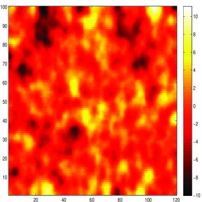
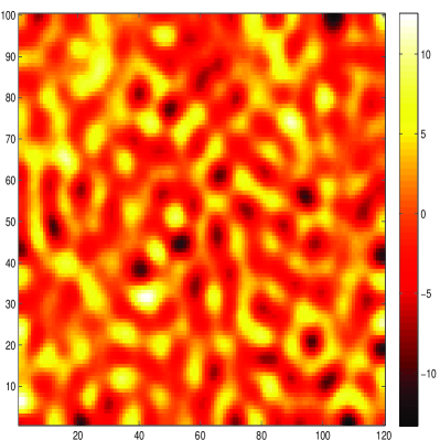
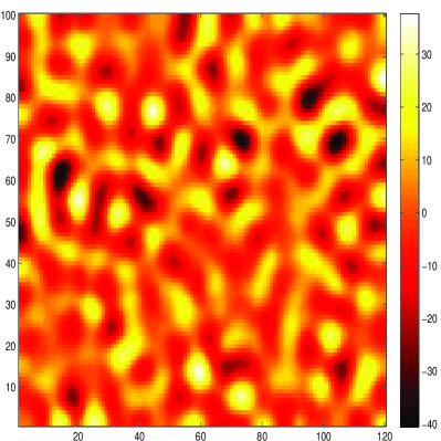
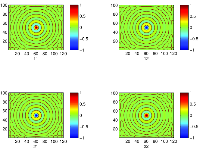
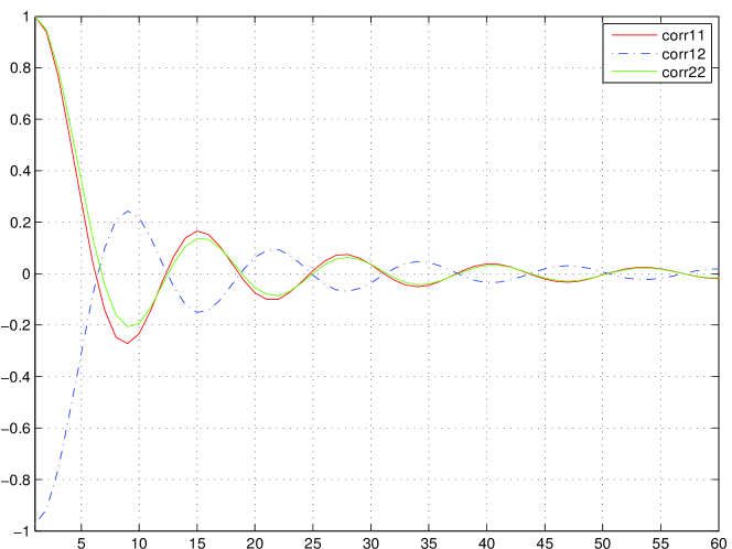
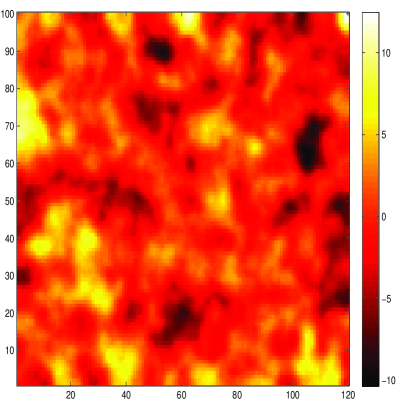
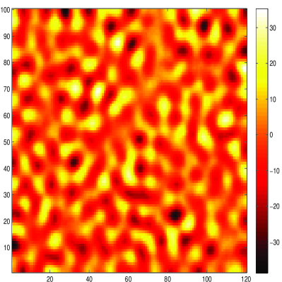
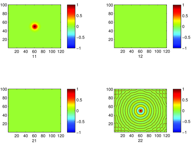
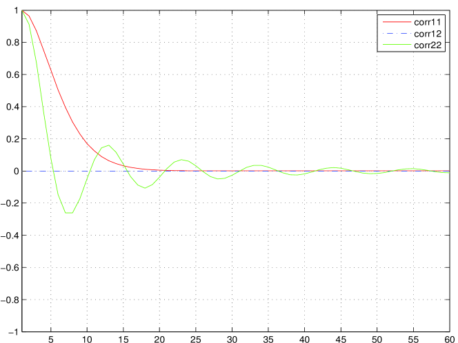
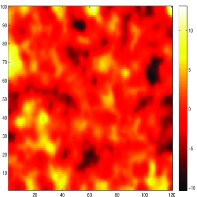
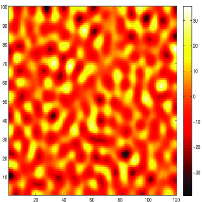
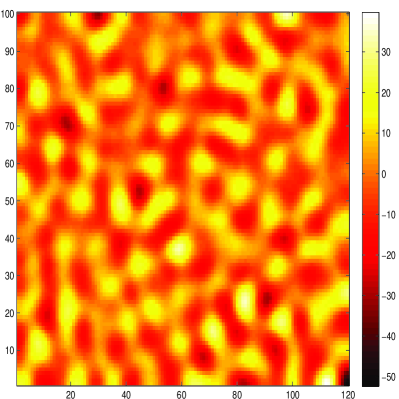
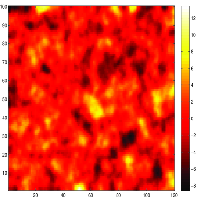
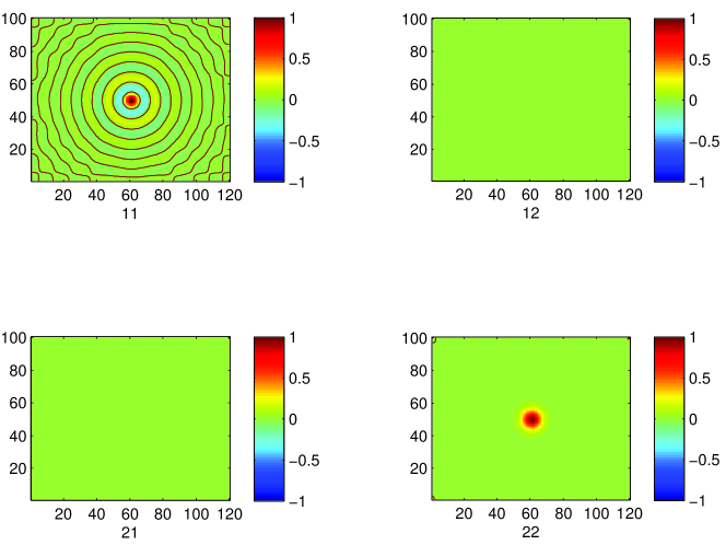
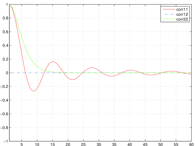
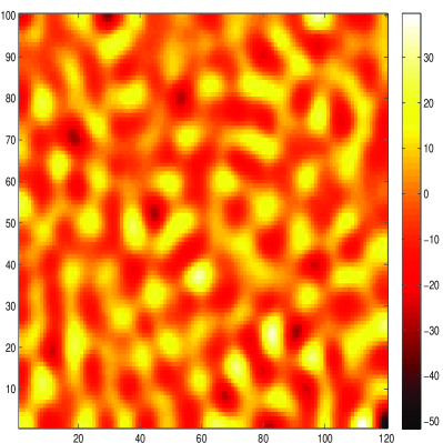
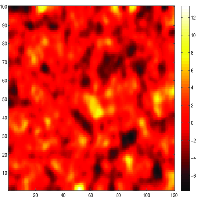
In the following two examples, we choose all values of parameters to be equal. However, we set to be a noise process with a non-oscillating covariance function and to be a noise process with an oscillating covariance function in the first example. In the second example, we simply switch the order of the noise processes, i.e., we set to be a noise process with an oscillating covariance function and to be a noise process with a non-oscillating covariance function.
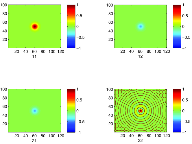
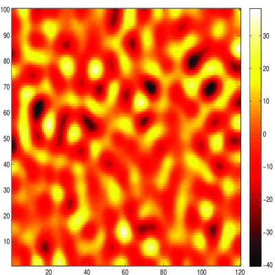
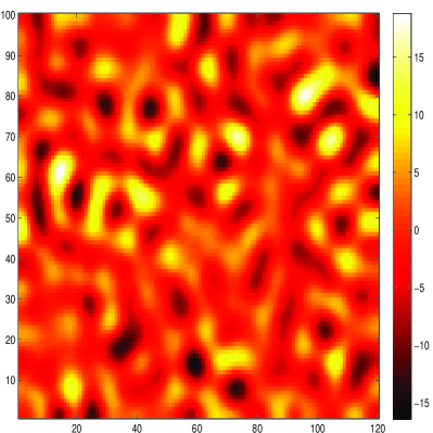
One sample from the GMRF in the first example is shown in Fig. 1 and one sample in the second example is shown in Fig. 4. The corresponding correlation matrices are shown in Fig. 2 and Fig. 5. In these figures, the red lines indicate that the correlation is . In the first example the random field has a non-oscillating covariance function and the second random field has an oscillating covariance function. In the second example both the fields have oscillating covariance functions. These two examples verify the conclusion in Section 3.3.
| Parameters | ||
|---|---|---|

4 Inference with simulated data and real data
In this section we illustrate how to use our approach with some simulated data examples and one real data example. In the first example, the covariance function of the first random field is non-oscillating, but the second random field has an oscillating covariance function. In the second example, both the random fields have oscillating covariance functions. The third and the forth examples show that if the two fields are independent, the inferences give indications about this, no matter which field is oscillating. One real data example in the end shows that our approach can be applied in practical applications. As pointed out by Diggle et al. (1998, Chapter 5) and Lindgren et al. (2011, Section 2), the smoothness parameter are poorly identifiable. Therefore, we fix the values of in the simulated data examples and in the real data example.
4.1 Posterior for the hyper-parameters
The first step of the inference is usually to derive the (log-) posterior distribution of . The well known Bayesian formula (36) is at the core of Bayesian inference,
| (36) |
where is the prior distribution of the hyper-parameters, and we return to this topic in Section 4.2, is the density for the bivariate random fields, is the density for the observations given the random field and the parameters and is the full conditional of the random fields given the observations and parameters.
Assume that there are triangles in the domain for each of the random field . With the bivariate random fields , triangles are used and hence the probability density of the bivariate random field has the form
| (37) |
where is the precision matrix for the bivariate field. We assume that the length of the data is , where are the length of the observations for each field. Then has the form
| (38) |
where is the precision matrix for the measurement errors with dimension , and is a matrix with dimension that links the sparse observations to the dense random fields. One thing we want to point out is that the length of the observations for each field can be different and they are not necessarily observed at the same locations. We used the notation instead of since this function is independent of . The full conditional can be obtained,
| (39) |
Denote , and . Then we have
| (40) |
Thus is a -dimensional multivariate Gaussian distribution. We can write (40) in the canonical form . For more information about canonical form of the GMRFs, we refer to, for example, Rue and Held (2005, Chapter 2).
| (41) |
And hence the logarithm of the posterior distribution is
| (42) |
4.2 Priors for the parameters
The prior distribution is important in Bayesian inference, and choosing the priors is an important part of inference. Two common approaches for choosing the prior distribution are the conjugate prior approach and the non-informative prior approach. There is no unique way for choosing priors. We refer to Robert (2007, Chapter 3) for detailed discussion about the prior information and prior distribution.
General speaking, it is hard to specify an informative prior for the hyper-parameters in our system of SPDEs approach. Therefore, the non-informative approach has been chosen. The following choice for the priors of the parameters are recommended with the bivariate random fields.
-
•
and should be positive values. So log-normal distributions are used for these two parameters. Gamma distribution can also be considered;
-
•
Because of the requirement on the systems of SPDEs that and should be positive values, we can use log-normal or gamma distributions;
-
•
is related to the sign of the correlation of the two random fields and it can be either positive or negative. Therefore, a Gaussian distribution can be used;
-
•
The oscillation parameter should fulfill the requirement and hence a beta distribution can be used.
4.3 Inference with simulated data
Four simulated data examples are presented in this section to illustrate how to use our proposed approach. The datasets are divided into groups. In the first group we use the correlated random fields given in Section 3.4. In the second group the fields are independent. We want our model to capture these features, and to return whether or not. However, if the first noise process is generated from the univariate SPDE given in Equation (2), and are not identifiable. See Appendix B for more information. We use the setting in this situation. It is our experience that is likely to be in the range of if we have empirical knowledge that the random field has an oscillating covariance function, and hence we recommend to use a beta distribution with negative skew. In all of our simulated data examples, we use the following priors for the parameters (if they are needed to be estimated) following the discussion given in Section 4.2.
-
•
have the log-normal distributions with and ;
-
•
has a normal distribution with and ,
-
•
has a beta distribution with and , , i.e., it is a uniform distribution.
The results for the first and second simulated datasets are given in Table 2 and Table 3, respectively. We can notice that the estimates are quite precise. Most of the true values are within standard derivation away from the estimates. None of the true values are standard deviations away from the estimates. The estimated conditional mean of the bivariate fields for these two datasets are given in Fig. 7 and Fig. 8. Compare with the true random fields given in Fig. 1 - Fig. 1 and Fig. 4 - Fig. 4. There is no large difference between them.
| Parameters | True values | Estimates | Standard deviations |
|---|---|---|---|
| 0.5 | 0.495 | 0.013 | |
| 0.25 | 0.248 | 0.017 | |
| 1 | 1.027 | 0.032 | |
| 0.25 | 0.248 | 0.010 | |
| 0.36 | 0.355 | 0.029 | |
| 0.6 | 0.601 | 0.004 | |
| 0.95 | 0.953 | 0.092 |
| Parameters | True values | Estimates | Standard deviations |
|---|---|---|---|
| 0.5 | 0.497 | 0.014 | |
| 0.25 | 0.234 | 0.012 | |
| 1 | 0.964 | 0.029 | |
| 0.25 | 0.269 | 0.024 | |
| 0.36 | 0.339 | 0.022 | |
| 0.5 | 0.496 | 0.005 | |
| 0.6 | 0.636 | 0.049 | |
| 0.95 | 0.956 | 0.113 |
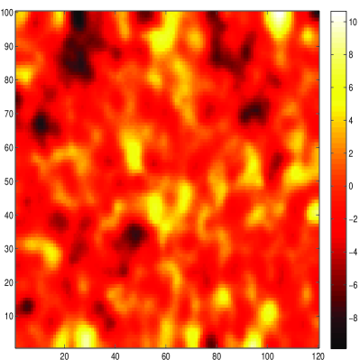

Similarly, the results for the second group are given in Table 4 and Table 5. In both examples, the estimates are precise and they are within standard derivations from the true values. We can notice that if the fields are independent, i.e., , our model captures this characteristic since is small and is within the credible interval.
| Parameters | True value | Estimated | Standard deviations |
|---|---|---|---|
| 0.5 | 0.491 | 0.012 | |
| 0 | 0.012 | 0.010 | |
| 0.3 | 0.301 | 0.010 | |
| 0.25 | 0.247 | 0.009 | |
| 0.36 | 0.374 | 0.033 | |
| 0.6 | 0.596 | 0.004 | |
| 0.95 | 0.951 | 0.092 |
| Parameters | True value | Estimated | Standard deviations |
|---|---|---|---|
| 0.5 | 0.487 | 0.015 | |
| 0 | 0.001 | 0.002 | |
| 0.3 | 0.308 | 0.009 | |
| 0.25 | 0.284 | 0.026 | |
| 0.36 | 0.359 | 0.122 | |
| 0.5 | 0.502 | 0.004 | |
| 0.6 | 0.599 | 0.102 | |
| 0.95 | 0.949 | 0.107 |
4.4 Inference with real data
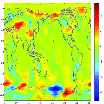
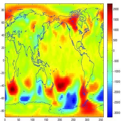
In this section a dataset has been chosen in order to illustrate how to use our approach in real-world applications. This dataset is from the ERA database and can be downloaded from the ERA project homepage. The dataset contains the temperature and pressure on the whole globe on th of September, . The main objective for this section is to illustrate how to use our model for a big dataset. All the results are only from the prediction point of view. The dataset contains observations both for temperature and pressure, and the observations are on the grid. The grid is constructed with the latitude and longitude. The latitudes are from to and longitudes are from to , with increments of for both axes. The dataset contains the temperatures in Kelvin and the mean sea level pressure in Pascal. We have subtracted the monthly mean for the temperature and pressure, respectively.
Since the dataset is on the entire globe, we need to construct our model on the sphere. Jones (1963) discussed how to construct stochastic processes on a sphere using the spectral representations for spherically symmetric and the axially symmetric cases. Another approach is to consider the sphere as a surface in . However, this has the disadvantage that the correlation between points are determined by the chordal distances (Lindgren et al., 2011). Gneiting (1998) pointed out that the random fields constructed on the plane were not suitable for this kind of dataset since the great circle distances in the original covariance function would not work in general. Jun and Stein (2007) discussed an approach for constructing space-time covariance functions on spheres using a sum of independent processes. The main idea for their approach is to sum independent processes where each process is obtained by applying the first-order differential operations to a fully symmetric processes on sphere time. We refer to Jun and Stein (2007) for more information on the fully symmetric processes on sphere time.
In this paper we follow the approach discussed by Lindgren et al. (2011) to construct the GRFs on the sphere. They claimed that using the SPDE approach for constructing GRFs on the sphere is similar to constructing the GRFs on . By reinterpreting the SPDE defined on , the solutions of the SPDE are GRFs defined on . Our proposed system of SPDEs approach inherits this property. The only place has been changed is that the system of SPDEs is directly defined on . Another advantage of our approach is that the GMRF approximation can still be used. In other words, we can use GMRFs to represent GRFs for computation. For more information about GRFs on manifolds, we refer to Lindgren et al. (2011, Section ).
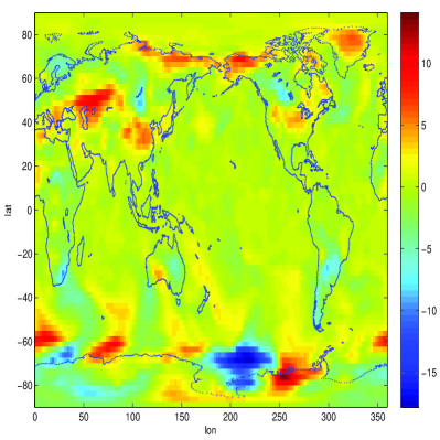
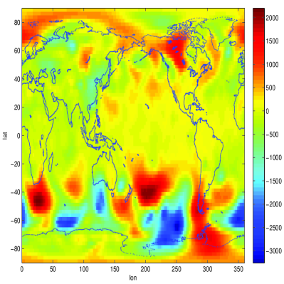
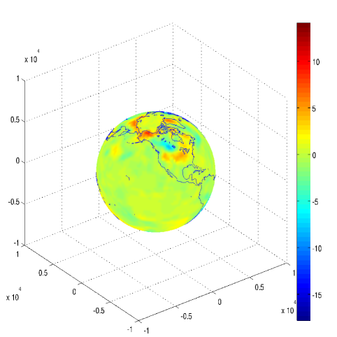
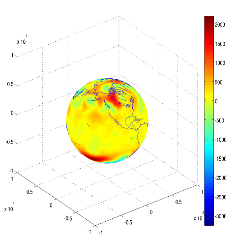
Since it is known that the pressure on the globe has an oscillating covariance function, it is reasonable to set as the temperature and as the pressure, and let the second noise process have an oscillating covariance function, but not the first noise process . The original dataset is shown in Fig. 17 and Fig. 17, and the reconstructed temperature and pressure are shown in Fig. 18 and Fig. 18. We also give images for the true datasets on the sphere in Fig. 19 and Fig. 19, and the reconstructed temperature and pressure on the sphere in Fig. 20 and Fig. 20. One thing we want to point out is that we follow the methodology given in Lindgren et al. (2011) and construct the GRF on the unit radius sphere . Another important point is that we set to simplify the model and inference.
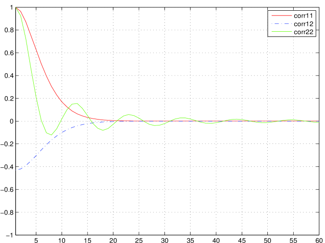
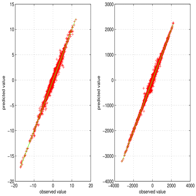
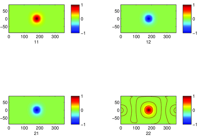
In order to check the predictive performance of our approach, we have divided the dataset into two subsets. We used a subset containing observations for both temperature and pressure for estimating the parameters and predict the remaining observations. The estimates are given in Table 6. From the results we notice that the model captures the empirical knowledge that the temperature and pressure are negative correlated since . The prediction for the observations are given in Fig. 21. From a prediction point of view, the model works well since most of the prediction are close to the true observed values. The correlation functions are given in Fig. 22, and we notice that the covariance function of pressure indeed has oscillation behavior.


| Parameters | Estimated |
|---|---|
5 Discussion and future work
Due to the increasing importance of spatial statistics in applications, new approaches for handling different complex datasets are demanded. The methodologies for dealing with multivariate datasets appear in many areas, such as in air quality (Brown et al., 1994; Schmidt and Gelfand, 2003), weather forecasting (Courtier et al., 1998; Reich and Fuentes, 2007), and economics (Gelfand et al., 2004; Sain and Cressie, 2007). Two of the most important issues with these methodologies are how to handle large datasets and how to ensure the nonnegative definiteness constraint for the covariance function. Gneiting et al. (2010) gave some theorems in order to construct valid covariance functions for multivariate random fields. In their approach every component in the matrix-valued covariance function was a Matérn covariance function. Hu et al. (2012a) proposed to use the systems of SPDEs to construct multivariate GRFs with isotropic and non-oscillating covariance functions. The summary paper by Sun et al. (2012) discussed the approaches for how to handle large datasets. They discussed several approaches such as separable covariance structures (Genton, 2007; Fuentes, 2006), covariance tapering (Furrer et al., 2006; Zhang and Du, 2008), likelihood approximations (Vecchia, 1988; Stein et al., 2004), fixed rank kriging and fixed rank filtering (Cressie and Johannesson, 2008; Cressie et al., 2010) and Gaussian Markov random fields approximation (Rue and Tjelmeland, 2002; Rue et al., 2004; Rue and Held, 2005; Rue et al., 2009; Lindgren et al., 2011).
This paper is an extension of Lindgren et al. (2011) and Hu et al. (2012a). The main contribution of this paper is the proposed approach for constructing multivariate random fields with oscillating covariance functions using systems of SPDEs. The main idea is to use noise processes with oscillating covariance functions in order to introduce oscillation in the covariance functions of the random fields. We recommend to use the triangular systems of SPDEs since these models have some advantages. For instance, we have fewer hyper-parameters and we can locate which random fields have non-oscillating, oscillating, possibly oscillating covariance functions. This approach can construct many models discussed by Hu et al. (2012a) if we set the oscillation parameter . It also inherit most of the advantages of the SPDE approach discussed by Lindgren et al. (2011) and systems of SPDEs approach discussed by Hu et al. (2012a).
The two main challenges in multivariate random fields mentioned above can be partially solved with our model. On the theoretical side, the covariance functions of the multivariate random fields fulfill the nonnegative definite constraint automatically. On the computational side, the GMRF representation makes the precision matrices to be sparse. Thus numerical algorithms for sparse matrices can be used for fast sampling and inference. Four simulated datasets and one real dataset have been used to illustrate how to use our approach in different situations. The results have illustrated the effectiveness of the proposed approach.
There are several possible extensions for further research, such as constructing non-stationary multivariate GRFs from the systems of SPDEs, and spatio-temporal models both in and on manifolds. It should also be possible to use the integrated nested Laplace approximation (INLA) framework (Rue et al., 2009) for doing inference for the multivariate GRFs. More applied work using the proposed approach is under development.
Appendix A
There are different kinds of parametrization for the system of SPDEs. The main idea is to change the operators in (26) and use a different parametrization as discussed in Section 3.3. Two intuitive operator matrices are
| (43) |
| (44) |
With (43) and (44) the correlations between the fields will be changed. The operator matrix given in (43) introduces more flexibility since we have one more parameter to control the range of cross-correlation. However, it might be hard to estimate all the parameters in this case. With operator matrix given in (44), we have fewer parameters in the model, but the correlation structure between the fields is simplified. The second random field has the same correlation range as the first field. These two systems can be use in different applications.
Appendix B
When we use the triangular systems of SPDEs, we need to set the constraint since when the first noise process is generated from Equation (2), they are not identifiable together. Write the system of equations for the bivariate random field given in (34) explicitly as
Assume the first noise process is generated by
| (45) |
We can now rewrite the first equation in system (34) as a system of equations
| (46) |
This system of equations can be rewritten into one equation with white noise as the driving process,
| (47) |
It is obvious that and are not identifiable from each other since and commute. Therefore, we suggest the constraint . However, if the first noise process is oscillating and is generated from Equation (19), we don’t need this constraint because they are identifiable. However, we still recommend to use this setting in order to simplify the inference.
References
- Banerjee et al. (2004) S. Banerjee, B.P. Carlin, and A.E. Gelfand. Hierarchical modeling and analysis for spatial data. Chapman & Hall, 2004. ISBN 158488410X.
- Bolin and Lindgren (2009) D. Bolin and F. Lindgren. Wavelet markov models as efficient alternatives to tapering and convolution fields. Technical report, Mathematical Statistics, Centre for Mathematical Sciences, Faculty of Engineering, Lund University, 2009.
- Bolin and Lindgren (2011) D. Bolin and F. Lindgren. Spatial models generated by nested stochastic partial differential equations, with an application to global ozone mapping. The Annals of Applied Statistics, 5(1):523–550, 2011.
- Brenner and Scott (2008) S.C. Brenner and L.R. Scott. The mathematical theory of finite element methods, volume 15. Springer Verlag, 2008.
- Brown et al. (1994) P.J. Brown, N.D. Le, and J.V. Zidek. Multivariate spatial interpolation and exposure to air pollutants. Canadian Journal of Statistics, 22(4):489–509, 1994.
- Courtier et al. (1998) P Courtier, E Andersson, W Heckley, J Pailleux, D Vasiljevic, M Hamrud, A Hollingsworth, F Rabier, and M Fisher. The ecmwf implementation of three-dimensional variational assimilation (3d-var). i: Formulation. Quarterly Journal of the Royal Meteorological Society, 124:1783–1807, 1998.
- Cressie and Johannesson (2008) N. Cressie and G. Johannesson. Fixed rank kriging for very large spatial data sets. Journal of the Royal Statistical Society: Series B (Statistical Methodology), 70(1):209–226, 2008.
- Cressie et al. (2010) N. Cressie, T. Shi, and E.L. Kang. Fixed rank filtering for spatio-temporal data. Journal of Computational and Graphical Statistics, 19(3):724–745, 2010.
- Cressie (1993) N.A.C. Cressie. Statistics for spatial data, volume 298. Wiley-Interscience, 1993.
- Diggle and Ribeiro Jr (2006) P.J. Diggle and P.J. Ribeiro Jr. Model-based Geostatistics. Springer, 2006.
- Diggle et al. (1998) P.J. Diggle, JA Tawn, and RA Moyeed. Model-based geostatistics. Journal of the Royal Statistical Society: Series C (Applied Statistics), 47(3):299–350, 1998. ISSN 1467-9876.
- Fuentes (2006) M. Fuentes. Testing for separability of spatial–temporal covariance functions. Journal of Statistical Planning and Inference, 136(2):447–466, 2006.
- Fuglstad (2010) G.A. Fuglstad. Approximating solutions of stochastic differential equations with gussian markov random fields. Technical report, Department of Mathematical Science, Norwegian University of Science and Technology, 2010.
- Fuglstad (2011) G.A. Fuglstad. Spatial modelling and inference with spde-based gmrfs. Master’s thesis, Department of Mathematical Sciences, Norwegian University of Science and Technology, 2011.
- Furrer et al. (2006) R. Furrer, M.G. Genton, and D. Nychka. Covariance tapering for interpolation of large spatial datasets. Journal of Computational and Graphical Statistics, 15(3):502–523, 2006.
- Gelfand et al. (2004) A.E. Gelfand, A.M. Schmidt, S. Banerjee, and CF Sirmans. Nonstationary multivariate process modeling through spatially varying coregionalization. Test, 13(2):263–312, 2004.
- Gelfand et al. (2010) A.E. Gelfand, P.J. Diggle, M. Fuentes, and P. Guttorp. Handbook of spatial statistics. CRC Press, 2010.
- Genton (2007) M.G. Genton. Separable approximations of space-time covariance matrices. Environmetrics, 18(7):681–695, 2007.
- Gneiting (1998) T. Gneiting. Simple tests for the validity of correlation function models on the circle. Statistics & probability letters, 39(2):119–122, 1998.
- Gneiting et al. (2010) T. Gneiting, W. Kleiber, and M. Schlather. Matérn Cross-Covariance Functions for Multivariate Random Fields. Journal of the American Statistical Association, 105(491):1167–1177, 2010. ISSN 0162-1459.
- Goff and Jordan (1988) J.A. Goff and T.H. Jordan. Stochastic modeling of seafloor morphology: Inversion of sea beam data for second-order statistics. Journal of Geophysical Research, 93(B11):13589–13, 1988. ISSN 0148-0227.
- Handcock and Stein (1993) M.S. Handcock and M.L. Stein. A Bayesian analysis of kriging. Technometrics, 35(4):403–410, 1993. ISSN 0040-1706.
- Hartman and Hössjer (2008) L. Hartman and O. Hössjer. Fast kriging of large data sets with Gaussian Markov random fields. Computational Statistics & Data Analysis, 52(5):2331–2349, 2008. ISSN 0167-9473.
- Hjelle and Dæhlen (2006) Ø. Hjelle and M. Dæhlen. Triangulations and applications. Springer Verlag, 2006.
- Hu et al. (2012a) X. Hu, D.P. Simpson, F. Lindgren, and H. Rue. Multivariate gaussian random fields using systems of stochastic partial differential equations. statistical report, Norwegian University of Science and Technology, 2012a.
- Hu et al. (2012b) X. Hu, D.P. Simpson, and H. Rue. Specifying gaussian markov random fields with incomplete orthogonal factorization using givens rotations. Technical report, Department of Mathematical Science, norwegian University of Science and Technology, 2012b.
- Jones (1963) R.H. Jones. Stochastic processes on a sphere. The Annals of mathematical statistics, 34(1):213–218, 1963.
- Jun and Stein (2007) M. Jun and M.L. Stein. An approach to producing space–time covariance functions on spheres. Technometrics, 49(4):468–479, 2007.
- Kaufman et al. (2008) C.G. Kaufman, M.J. Schervish, and D.W. Nychka. Covariance tapering for likelihood-based estimation in large spatial data sets. Journal of the American Statistical Association, 103(484):1545–1555, 2008.
- Kloeden and Platen (1999) P.E. Kloeden and E. Platen. Numerical solution of stochastic differential equations. Springer, 3rd edition, 1999. ISBN 3540540628.
- Lindgren et al. (2011) F. Lindgren, H. Rue, and J. Lindström. An explicit link between gaussian fields and gaussian markov random fields: the stochastic partial differential equation approach. Journal of the Royal Statistical Society: Series B (Statistical Methodology), 73(4):423–498, 2011.
- Lindgren (2010) G. Lindgren. A second course on stationary stochastic processes. Center for Mathematical Sciences, Lund University, December 2010.
- Matérn (1986) B. Matérn. Spatial variation. Springer-Verlag Berlin, 1986.
- Reich and Fuentes (2007) B.J. Reich and M. Fuentes. A multivariate semiparametric bayesian spatial modeling framework for hurricane surface wind fields. The Annals of Applied Statistics, 1(1):249–264, 2007.
- Robert (2007) C. Robert. The Bayesian choice: from decision-theoretic foundations to computational implementation. Springer Verlag, 2007.
- Rue (2001) H. Rue. Fast sampling of Gaussian Markov random fields. Journal of the Royal Statistical Society: Series B (Statistical Methodology), 63(2):325–338, 2001. ISSN 1467-9868.
- Rue and Held (2005) H. Rue and L. Held. Gaussian Markov random fields: theory and applications. Chapman & Hall, 2005. ISBN 1584884320.
- Rue and Tjelmeland (2002) H. Rue and H. Tjelmeland. Fitting Gaussian Markov random fields to Gaussian fields. Scandinavian Journal of Statistics, 29(1):31–49, 2002. ISSN 1467-9469.
- Rue et al. (2004) H. Rue, I. Steinsland, and S. Erland. Approximating hidden Gaussian Markov random fields. Journal of the Royal Statistical Society: Series B (Statistical Methodology), 66(4):877–892, 2004. ISSN 1467-9868.
- Rue et al. (2009) H. Rue, S. Martino, and N. Chopin. Approximate Bayesian inference for latent Gaussian models by using integrated nested Laplace approximations. Journal of the Royal Statistical Society: Series B (Statistical Methodology), 71(2):319–392, 2009. ISSN 1467-9868.
- Sain and Cressie (2007) S.R. Sain and N. Cressie. A spatial model for multivariate lattice data. Journal of Econometrics, 140(1):226–259, 2007.
- Schmidt and Gelfand (2003) A.M. Schmidt and A.E. Gelfand. A bayesian coregionalization approach for multivariate pollutant data. Journal of Geophysical Research, 108(D24):8783, 2003.
- Shaby and Ruppert (2012) B. Shaby and D. Ruppert. Tapered covariance: Bayesian estimation and asymptotics. Journal of Computational and Graphical Statistics, 21(2):433–452, 2012.
- Stein (1999) M.L. Stein. Interpolation of Spatial Data: some theory for kriging. Springer Verlag, 1999. ISBN 0387986294.
- Stein et al. (2004) M.L. Stein, Z. Chi, and L.J. Welty. Approximating likelihoods for large spatial data sets. Journal of the Royal Statistical Society: Series B (Statistical Methodology), 66(2):275–296, 2004.
- Sun et al. (2012) Y. Sun, B. Li, and M.G. Genton. Geostatistics for large datasets. Advances and challenges in space-time modelling of natural events, pages 55–77, 2012.
- Vecchia (1988) A.V. Vecchia. Estimation and model identification for continuous spatial processes. Journal of the Royal Statistical Society. Series B (Methodological), pages 297–312, 1988.
- Wei (2006) W.W.S. Wei. Time series analysis: univariate and multivariate methods. Addison-Wesley, 2006.
- Whittle (1954) P. Whittle. On stationary processes in the plane. Biometrika, 41(3-4):434–449, 1954. ISSN 0006-3444.
- Whittle (1963) P. Whittle. Stochastic processes in several dimensions. Bull. Int. Statist. Inst., 40:974–994, 1963.
- Zhang and Du (2008) H. Zhang and J. Du. Covariance tapering in spatial statistics. Positive definite functions: From Schoenberg to space-time challenges, pages 181–196, 2008.
- Zienkiewicz et al. (2005) O.C. Zienkiewicz, R.L. Taylor, R.L. Taylor, and JZ Zhu. The finite element method: its basis and fundamentals, volume 1. Butterworth-heinemann, 2005.