Link-weight distribution of microRNA co-target networks
exhibit universality

Abstract

MicroRNAs (miRNAs) are small non-coding RNAs which regulate gene expression by binding to the $3^{\prime}$ UTR of the corresponding messenger RNAs. We construct miRNA co-target networks for $22$ different species using a target prediction database, MicroCosm Tagets. The miRNA pairs of individual species having one or more common target genes are connected and the number of co-targets are assigned as the weight of these links. We show that the link-weight distributions of all the species collapse remarkably onto each other when scaled suitably. It turns out that the scale-factor is a measure of complexity of the species. A simple model, where targets are chosen randomly by miRNAs, could provide the correct scaling function and explain the universality.

I Introduction

Biological functions occur in living cells through bio-chemical interactions of proteins. It is a central dogma cdogma of molecular biology that protein synthesis occurs inside the cell in two steps, (i) transcriptions, where information from genes are transfered to the messenger RNA (mRNA) and (ii) translation, where information coded in mRNA is translated into specific sequence of amino acids (proteins). The protein densities in the cell are primarily regulated by transcription factors TF , however recent studies book ; farh show that a set of small non-coding single stranded RNAs, namely micro-RNAs (miRNAs), also act as secondary regulators. MicroRNAs are produced from either their own genes or from introns. MicroRNAs are about $20$ nucleotides long, they usually bind to the $3^{\prime}$ UTR of the mRNA inhibiting their functionality. Several computational tools majoros ; grimson have been developed to identify, firstly the genomic sequences which can transcribe miRNAs and their possible targets. It has been estimated that Homo sapiens have $851$ miRNAs miRBase and their predicted targets constitute about $90\%$ of the total genes miranda . Experimental validation of such predictions are, however, largely lacking.

Being a secondary regulator, miRNAs usually repress the gene expression marginally. Thus it is natural to expect that cooperative action of miRNAs are needed for alteration of any biological function or pathway. Recent studies xu have revealed this co-operativity using miRNA co-target networks, constructed by taking miRNAs as nodes connected by weighted links where the weight corresponds to the common targets of the connecting pair. Apparently $50\%$ miRNAs in Homo sapiens provide all essential regulations by forming several small miRNA clusters mookherjee . Study of miRNA co-target networks for different species reveal that these networks are quite similar and are robust against random deletion of nodes Lee .

Figure 1: Schematic miRNA co-target network of an example species having $N=7$ genes and $M=5$ miRNAs. The bipartite network (left) shows genes, targeted miRNAs. The miRNA co-target network (right) is formed by joining miRNA pairs which have at least one common target. The weights (number of co-targets) are written beside each link.

In this article we show that the distributions of weights of miRNA co-target networks are strikingly universal. The universality can be explained through a simple model that assumes unbiased binding of miRNAs with the available mRNAs. Since species have different number of miRNA and genes, the mean and standard deviations (SD) of their weight distributions naturally differ. However, the distributions are related to each other through a simple scaling indicating that the underlying binding mechanism is unbiased.

II MiRNA co-target network

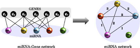
To construct the miRNA co-target network we use a web resource MicroCosm Targets microcosm which provides computationally predicted targets of microRNAs across many species. To predict the targets MicroCosm uses the miRNAs sequences from a well known miRNA prediction database miRBase miRBase and genomic sequences from EnsEMBL EnsEMB . The number of predicted miRNAs $M$ and the total number of genes $N$ are listed in Table 1 for $22$ different species. Note that the species considered here are quite sparse with respect to their class. For all the species, a miRNA can target several genes and a gene can also be targeted by several miRNAs. This gives rise to the possibility that a pair of miRNA can have more than one common targets or co-targets. The co-target network is constructed separately for each species by taking their miRNAs as nodes. A miRNA pair having $w>0$ number of common target genes are then connected if by a link of weight $w$. The detailed procedure is described schematically in the fig. 1.

Figure 2: (a) The link-weight distributions $P(w)$ for some representative species. (b) The peak position $w^{*}$ depends linearly on the number of genes $N;$ the best fitted line has slope $=0.0012(1)$ and $y$-intercept $=-8.021$.

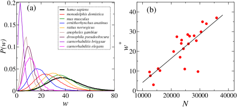
In these networks the weight of the links, i.e. the number of co-targets of a pair of miRNAs, vary in a wide range. For Homo sapiens the weights are bounded in the range $1\leq w\leq 1282$, whereas it varies in a smaller range $1\leq w\leq 513$ for C. Elegans. The distribution function $P(w)$ of the weights $w$ are calculated separately for $22$ species. Figure 2(a) shows $P(w)$ vs. $w$ for some representative species. All these distribution functions show a single peak at some value of $w$, say $w^{*}$, which is different for different species. The values of $w^{*}$ are also listed in Table 1. It is natural to expect a higher $w^{*}$ for the species which has larger number of genes. We find, to a reasonable approximation, that $w^{*}$ varies linearly with the number of respective genes $N$ (see fig. 2(b)).

Table 1: List of species studied here.

Sl.	Species (cell types types )	M	N	$w^{*}$	$\lambda$	$\bar{n}$	$s$
1	Aedes aegypti (-)	82	16059	10.2	0.32	388.71	47.94
2	Anopheles gambiae (65)	82	12708	7.6	0.25	303.33	38.39
3	Drosophila pseudoobscura (-)	88	12416	9.5	0.30	247.67	38.79
4	Drosophila melanogaster (63)	93	15416	11.2	0.34	392.31	55.53
5	Caenorhabditis briggsae (35)	135	13785	3.0	0.15	161.45	37.39
6	Caenorhabditis elegans (35)	136	24728	11.0	0.40	513.04	84.90
7	Gasterosteus aculeatus (-)	172	26423	27.7	0.65	824.63	111.07
8	Oryzias latipes (-)	172	23514	24.0	0.59	729.27	98.42
9	Takifugu rubripes (120)	173	21972	27.4	0.64	761.92	97.76
10	Tetraodon nigroviridis (120)	174	28005	27.9	0.63	828.94	100.69
11	Xenopus tropicalis (130)	199	24272	21.3	0.58	669.93	96.35
12	Danio rerio (120)	233	28744	25.4	0.62	792.40	103.90
13	Monodelphis domestica (-)	644	26013	23.8	0.79	799.11	150.23
14	Gallus gallus (152)	651	20842	19.9	0.58	608.95	86.90
15	Macaca mulatta (-)	656	32302	34.0	0.88	954.25	141.03
16	Pan troglodytes (175)	662	29355	9.7	0.32	227.16	32.08
17	Canis familiaris (160)	668	23628	25.7	0.78	768.99	124.87
18	Ornithorhynchus anatinus (-)	668	23097	17.0	0.59	624.54	117.07
19	Bos taurus (-)	676	25759	28.5	0.82	814.99	126.36
20	Rattus norvegicus (160)	698	30421	29.9	0.75	891.74	131.47
21	Mus musculus (160)	793	30484	35.0	0.84	885.63	127.49
22	Homo sapiens (175)	851	35864	37.0	1.00	959.03	147.03

III Universality

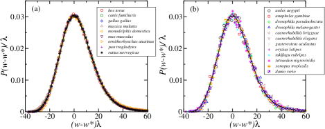
The distribution functions $P(w)$s show an interesting scaling behaviour, $i.e.$ they could be collapsed onto a unique scaling function, even though a large diversity is present among the species. To observe the collapse, the distribution functions are first shifted using a linear transformation $w\rightarrow w-w^{*}$ which bring the peaks of $P(w)$ to origin and then both the axises are re-scaled suitably using a scaling parameter $\lambda$. The probability density function (PDF) obeys a scaling relation $P(\lambda w)=P(w)/\lambda$ to assure the normalization $\int_{0}^{\infty}P(w)dw=1.$ Thus a linear shift and a re-scaling, done here, does not alter the functional form. In fig. 3(a) we have plotted $P(w-w^{*})/\lambda$ vs. $(w-w^{*})\lambda$ for species having larger number of miRNAs $M>300,$ where $\lambda$ is chosen such that the shifted distribution functions are collapsed best on to the unscaled data of one of the species (here Homo sapiens). Data-collapse for species having lesser number of miRNAs $M<300$ are shown separately in fig. 3(b) as they have large fluctuations which obstruct the visual clarity. Clearly, the rescaled $P(w)$ in both figures matches remarkably with the PDF for Homo sapiens $P_{h}(w)$ (shown as a thick solid line). This suggests that a universal functional form governs the distribution of number of co-targets across a wide class of species, even though, the miRNAs and their predicted targets are quite different among species.

Figure 3: $P(w)$ for (a) species with $(M>300)$ and (b) the rest, are collapsed onto the distribution curve for Homo sapiens (solid line). Note that in (b) the fluctuation is larger as these species has lower number of miRNAs.

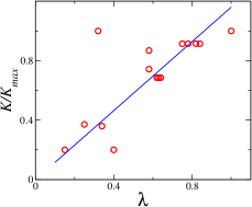
At this point the following comment is in order : the scale-factor $\lambda$ (see Table 1) used for collapsing $P(w)$s of different species can be considered as a measure of morphological complexity in animal evolution. In fig. 4 we plot $\lambda$ versus the number of cell types $K$ of the respective species types and find that, to a good approximation, they are proportional. Thus like the number of cell types, which is usually considered as a species complexity types , $\lambda$ can also be used as an equivalent measure. We will see later, from a simple model, that $\lambda$ for a given species is related to the fraction of the total genes typically targeted by its miRNAs.

Figure 4: The scale factor $\lambda$ is proportional the number of cell types $K$ (here normalized by $K_{max}=175).$ The proportionality constant is $1.16(8).$

The distribution of number of co-targets $P(w)$ for all the species studied here are only a scaled form of a unique scaling function ${\cal F}(w)$. To find out this universal scaling form we make an ansatz,

$${\cal F}(w)=g(w)G(w;\mu)$$

where $G(w;\mu)$ is a normal distribution with mean $\mu$ and standard deviation $\sigma=1$. The term $f(w)$ take care of the deviation from normal distribution, which has a Taylor’s series about $w=\mu,$

$$g(w)=g(\mu)-\alpha(w-\mu)+{\cal O}((w-\mu)^{2}),$$ (1)

where $\alpha\equiv-g^{\prime}(\mu).$ Clearly to the $0^{th}$ order, ${\cal F}(w)=g(\mu)G(w;\mu).$ Since $G(w;\mu)$ is already normalized, we have $g(\mu)=1.$ To the next order in $(w-\mu),$

$${\cal F}(w)={1\over\sqrt{2\pi}}\left[1-\alpha(w-\mu)\right]e^{-{{(w-\mu)^{2}}\over{2}}}.$$ (2)

In the present study we will restrict ourself only to the above form of ${\cal F}(w)$ and argue that $P(w)$ for different species can be obtained through scaling

$$P(w)={1\over\Lambda}{\cal F}({w\over\Lambda}),$$ (3)

where $\Lambda$ is species dependent. The maximum (or the peak) of the scaling function ${\cal F}(w)$ occurs at $w=\mu^{*}$ where ${\cal F}^{\prime}(\mu^{*})=0.$ We find that $\mu^{*}=\mu-\Delta$ where

$$\Delta=\frac{\sqrt{1+4\alpha^{2}}-1}{2\alpha}~{}~{}{\rm(equivalently,}~{}~{}\alpha=\frac{\Delta}{1-\Delta^{2}})$$ (4)

is positive, indicating that the added term $g(w)$ shifts peak of the normal distribution to left. Thus ${\cal F}(w)$ can be expressed in terms of $\mu^{*}$ as

$${\cal F}(w)={1\over\sqrt{2\pi}}\left[1-\alpha(w-\mu^{*}-\Delta)\right]e^{-(w-\mu^{*}-\Delta)^{2}/2}.$$ (5)

The remaining task is to determine the parameters $\alpha$ (a measure of skewness) and $\mu^{*}$ (peak position) from the co-target distribution data. However, the distribution functions can not be used directly as they are scaled forms of ${\cal F}(w)$ (see eq. (5)) and the corresponding scale factors are not known. In fact it is enough to determine only the scale factor $\hat{\Lambda}$ that relates $P_{h}(w)$ with ${\cal F}(w);$ $P(w)$ of all other species which are already collapsed onto $P_{h}(w)$ through $\lambda$ listed in Table 1, can also be collapsed onto ${\cal F}(w)$ using $\Lambda=\lambda\hat{\Lambda}.$ But, $P_{h}(w)={1\over\hat{\Lambda}}{\cal F}({w\over\hat{\Lambda}})$ has two unknown parameters $\hat{\Lambda}$ and $\alpha$ which need to be determined simultaneously. Note, that $\mu^{*}$ can be calculated from knowing $\hat{\Lambda}$ as $P_{h}(w)$ has its peak at $w^{*}=\hat{\Lambda}\mu^{*}=37$ (see Table 1). We proceed by expanding $P_{h}(w)$ in Taylor’s series about $w=w^{*};$ to the leading order,

$$P_{h}(w)=\frac{1}{\hat{\Lambda}}\left[{\cal F}(\mu^{*})+\frac{(w/w^{*}-1)^{2}}{\hat{\Lambda}^{2}}{w^{*}}^{2}{\cal F}^{{}^{\prime\prime}}(\mu^{*})\right].$$ (6)

Thus the plot of $P_{h}(w)$ versus $(w/w^{*}-1)^{2}$ is expected to be linear near the peak with slope $m={w^{*}}^{2}{\cal F}^{{}^{\prime\prime}}(\mu^{*})/\Lambda^{3}$ and $y$-intercept $c={\cal F}(\mu^{*})/\Lambda.$ In fig. 5(a) we have shown this plot for Homo sapien (larger dots). The weight distribution of all other species, after collapsing on to $P_{h}(w),$ are also plotted in the same graph to obtain a better estimates of $m$ and $c.$ The best fitted line, gives slope $m=-0.115$ and $y$- intercept $c=0.030.$ However, from eqs. (5) and (6) we know that

$$c=\frac{e^{-\Delta^{2}/2}}{\sqrt{2\pi}\hat{\Lambda}(1-\Delta^{2})}~{}~{}{\rm and}~{}~{}m=-\frac{{w^{*}}^{2}(1+\Delta^{2})}{2\hat{\Lambda}^{2}}c~{},$$ (7)

Evidently $\frac{m}{c^{3}}$ is independent of $\Lambda$ and for $\Delta\ll 1$ it can be approximated as $\frac{m}{c^{3}}\simeq{w^{*}}^{2}\pi(1-3\Delta^{4}/2).$ Using the values of $c,m$ and $w^{*}=37$ we have

$$\hat{\Lambda}=13.888,~{}\Delta=0.283;$$ (8)

$${\rm and} \mu^{*}=\frac{w^{*}}{\hat{\Lambda}}=2.664,~{}\alpha=0.308.$$ (9)

Figure 5: (a) Weight distribution $P_{h}(w)$ for Homo sapiens (larger dots) versus $(w/w^{*}-1)^{2}$ is linear with slope $m=-0.115$ and $y$-intercept $c=0.030$. The small dots denote $P(w)$ of other species after being collapsed to $P_{h}(w).$ (b) The scaled distribution $\Lambda P(\Lambda w)$ (dots), where $\Lambda=13.888\lambda$ taken from Table 1), is compared with the universal function ${\cal F}(w),$ (eq. (5)). Different colours (dots) are used for species $M<300$ and the rest.

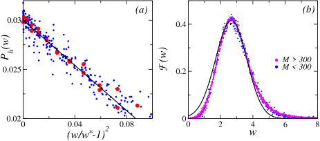
The universal scaling function ${\cal F}(w)$ is now specified completely. In fig. 5 (b) we compare ${\cal F}(w)$ with $\Lambda P(w\Lambda)$ using $\Lambda=\hat{\Lambda}=13.888$ for Homo sapien and $\Lambda=\lambda\hat{\Lambda}$ for others, where $\lambda$ is taken from Table 1. Clearly the distributions collapse onto each other and match reasonably well with ${\cal F}(w);$ the small discrepancy observed for $|w-\mu^{*}|\gg 1$ can possibly be improved by taking higher order terms of $g(w)$ in eq. (1).

IV Model

In the previous section we proposed a universal scaling function ${\cal F}(w)$ which on rescaling agrees reasonably well with the weight distribution $P(w)$ of miRNA co-target networks. It is only that the scale factors differ among the species. ${\cal F}(w)$ has two parameters $\alpha$ and $\mu^{*}$ which could be determined from the weight distribution data. Here we introduce a simple microscopic model to understand the origin of the scale factors $\Lambda$ and the constants $\alpha$ and $\mu^{*}.$ In other words we would like to understand the dependence of $\Lambda$, $\alpha$ and $\mu^{*}$ on the number of miRNAs $M,$ the number genes $N,$ and the average number of targets $\bar{n}$ of a given species.

Let $M$ miRNAs of a concerned species be labeled by $i=1,2,\dots M$ and each miRNA $i$ targets $n_{i}$ genes out of total $N$. Although in reality, the miRNAs target specific genes depending on whether it can bind to the $3^{\prime}$ UTR of the mRNA (of the concerned gene), in this model we consider that the targets are chosen randomly, $i.e.$ each miRNA $i$ target $n_{i}$ genes out of total $N$ genes where $n_{i}$ is a stochastic variable drawn from distribution $\phi(n)$. Since, miRNAs bind to the $3^{\prime}$ UTR of mRNAs, based on the sequence matching and binding energies, targets of one miRNA is largely uncorrelated with the targets of the other. Thus, in this random target model, it is reasonable to assume that $\phi(n)$ is a normal distribution with mean $\bar{n}$ and SD $s;$ subsequently we denote $\phi(n)\equiv\phi(n;\bar{n},s).$ These simple assumptions may not sound very realistic, however we show that it captures the basic features of the weight distribution $P(w)$ remarkably well.

Clearly, $n$ transcripts can be chosen out of $N$ in $C^{N}_{n}$ possible ways. Thus, the probability that there are $w$ common targets among a pair of miRNAs, say $i=1$ and $2$, is given by

$$Q_{N}(w,n_{1},n_{2})=\frac{C^{n_{1}}_{w}C^{N-n_{1}}_{n_{2}-w}}{C^{N}_{n_{2}}}\;.$$ (10)

Accordingly, the distribution of common targets is

$$P(w)=\sum_{n_{1},n_{2}=w}^{N}Q_{N}(w,n_{1},n_{2})\phi(n_{1};\bar{n},s)\phi(n_{2};\bar{n},s).$$ (11)

In the continuum limit, using rescaled variables $\nu_{1,2}=n_{1,2}/N,$ $x=w/N,$ $\bar{\nu}=\bar{n}/N,$ and $\sigma=s/N$ the sum is converted to an integral

$$P(x)=\int_{x}^{1}d\nu_{1}\int_{x}^{1}d\nu_{2}Q(x,\nu_{1},\nu_{2})\phi(\nu_{1})\phi(\nu_{2})\;,$$ (12)

where all the functions $P$ and $\phi$ scales as $f(n=\nu N)\to f(\nu)/N.$ The functional form of $Q(x,\nu_{1},\nu_{2})$, in the large $N$ limit, can be obtained from eq. (10), using Stirling approximation,

$$Q(x,\nu_{1},\nu_{2})=\sqrt{N\over 2\pi}g(x,\nu_{1},\nu_{2})e^{-NS(x,\nu_{1},\nu_{2})}\;\;,$$ (13)

with $S(x,\nu_{1},\nu_{2})=f(1-\nu_{1}-\nu_{2}+x)+f(\nu_{1}-x)+f(\nu_{2}-x)+$
$f(x)-f(\nu_{1})-f(1-\nu_{1})-f(\nu_{2})-f(1-\nu_{2}),$ $f(x)=x\ln x,$
and $g(x,\nu_{1},\nu_{2})=\left[{\nu_{1}\nu_{2}(1-\nu_{1})(1-\nu_{2})\over x(1-\nu_{1}-\nu_{2}+x)(\nu_{1}-x)(\nu_{2}-x)}\right]^{1\over 2}.$

Figure 6: Target distribution $\phi(m)$ of miRNAs for (a) Homo sapiens and (b) C. elegans are fitted to a Gaussian function (lines) with mean and SD ($\bar{n}$, $s$) = $(959.0,147.0)$ and $(513.0,84.9)$ respectively.

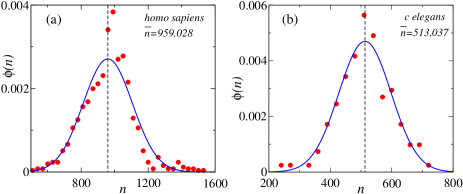
To proceed further, we need to specify $\phi(n),$ the distribution of the number of genes $n$ targeted by the miRNAs of a given species. We have calculated this distribution $\phi(n)$ for all the $22$ species; a plot of $\phi(n)$ is shown in fig. 6(a) and (b) for Homo sapiens and C. elegans respectively. The distribution $\phi(n)$ is too noisy as the sample space (total number of number of miRNAs of a given species) is too small. Hence, it produces a large error in the estimates of the mean $\bar{n}$ and SD $s,$ when fitted to a normal-distribution. Moreover, we find that the ratio of $s$ and $\bar{n}$ is close to $15\%$ for all the species. This indicates that, for any species, about $84\%$ of the number of targets deviate at most $15\%$ from the mean $\bar{n}$. Thus, for simplicity, one may assume the distribution to be $\phi(n)=\delta(n-a).$ In the following, we present the results for this choice, as it simplifies eq. (12) substantially and provides a closed form expression of ${\cal F}(w).$ There is no specific difficulty in considering $\phi(n)$ as a normal distribution with finite width $s$; it only scales the values of $\alpha$ and $\mu^{*}$ by a $s$-dependent factor.

For $\phi(\nu)=\delta(\nu-\bar{\nu})$, i.e. when every miRNA of a species target the same number of genes, $P(x)=Q(x,\bar{\nu},\bar{\nu})$ is significant only near $x=\bar{\nu}^{2}$ where $S(x,\bar{\nu},\bar{\nu})$ has its minima. Expanding both $S(x,\bar{\nu},\bar{\nu})$ and $g(x,\bar{\nu},\bar{\nu})$ in a Taylor’s series about $x=\bar{\nu}^{2}$ upto the leading order we get,

$$P(x)=\frac{1}{\sqrt{2\pi}\Omega}\left[1-\frac{(1-2\bar{\nu})^{2}}{2N\Omega^{2}}(x-\bar{\nu}^{2})\right]e^{-{(x-\bar{\nu}^{2})^{2}}\over{2\Omega^{2}}},$$

where $\Omega=\bar{\nu}(1-\bar{\nu})/\sqrt{N}.$ Since $x=w/N$, the weight distribution $P(w)$ is related to ${\cal F}(w)$ in eq. (5) by the scale factor $\Lambda=\Omega N,$ where

$$\Lambda=\frac{\bar{n}(N-2\bar{n})}{N^{3/2}};\alpha=\frac{(N-2\bar{n})^{2}}{2\sqrt{N}\bar{n}(N-\bar{n})};\mu^{*}+\Delta=\frac{\bar{n}^{2}}{N\Lambda}.$$ (14)

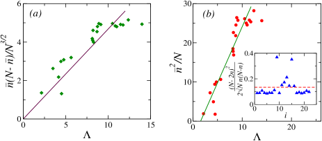
In fig. 7(a) we have shown $\bar{n}(N-2\bar{n})/N^{3/2}$ as a function of $\Lambda$ and find that they are proportional, but the proportionality constant is $0.468$ instead of unity. Note that the scale-factor is a measure of the complexity of a species and now it can be expressed as $\Lambda\simeq\bar{\nu}\sqrt{N}$ because $\bar{\nu},$ which represents the fraction of genes typically targeted by the miRNAs of a species, is usually small (refer to Table -1). Therefore only the gene number is not an indicative of species complexity; the complexity also depends on ‘what fraction of those genes are targeted by miRNAs’.

In the fig. 7(b) we have also shown $\bar{n}^{2}/N$ as a function of $\Lambda$ and fit the data to a straight line. It follows from eq. (14) that the slope is $\mu^{*}+\Delta=2.858.$ In the inset of this figure we plot $\alpha,$ calculated using above equation, for all the species; the average value $\alpha=0.135$ is shown as a horizontal line. Finally using this value of $\alpha$ in eq. (4) we get $\mu^{*}=2.858-\Delta=2.725.$ Clearly there is large fitting error in these estimates of $\mu^{*}$ and $\alpha$ and they deviate a bit from the values obtained in eq. (9). However, given the simplicity of the model where target distribution is taken as a $\delta$-function, it is rather surprising that the estimates are of the same order of magnitude as compared to eq. (9). The difference may be recovered from adding a finite width $s$ to the target distribution as $s$ simply rescales the parameters $\alpha$ and $\mu^{*}$ (calculations are not shown here).

Figure 7: (a) Scaling parameter $\Lambda=13.888\lambda$ is proportional to $\bar{n}(N-\bar{n})/N^{3\over 2},$ but the proportionality constant $0.468$ is different from unity (eq. (14)) (b) $\Lambda$ versus $\bar{n}^{2}/N$ is linear with slope $(\mu^{*}+\Delta)=2.54.$ Inset shows $\frac{(N-2\bar{n})^{2}}{2\sqrt{N}\bar{n}(N-\bar{n})}$ for all species and their average is $\alpha=0.135$ (horizontal line).

V Conclusion

In this article we construct miRNA co-target networks of $22$ different species, using the predicted miRNA targets from MicroCosm Target database microcosm . A pair of miRNA are connected, only if they have at least one common target; number of co-targets are considered as the weight of the link. To our surprise, we find that the link-weight distribution of $22$ different species show an spectacular data collapse under scaling. Using scaling arguments we obtain an universal scaling function ${\cal F}(x)$ with two parameters: $\mu^{*}$ for peak position, and $\alpha$ for skewness. The weight distribution functions $P(w)$s are only a scaled form of this function, $i.e.,~{}P(w)={\cal F}(w/\Lambda)/\Lambda;$ the scale-factors $\Lambda$ varies with species and it may be considered as measure of complexity (number of cell types of a species types ).

To explain the universality, we propose a simple model where miRNAs of a given species are assumed to target a fixed number of genes. This random target model could provide the correct functional form of ${\cal F}(x)$ and estimate the parameters $\alpha$ and $\mu^{*}$ reasonably well. Discrepancy in these estimates may be substantiated by taking the distribution of the number of individual miRNA targets as a Gaussian distribution with finite width. The model also predicts that the scale-factor, which is a measure of species complexity, depends on both of the number of genes, and the fraction of genes typically targeted by the miRNAs of that species.

It is rather surprising, why such a simple model captures the functional form of the weight distribution of miRNA co-target network. Being the regulators of transcription, individual or group of miRNAs of a given species cooperatively target one or more genes for carrying out required functions. Thus, the miRNA binding is much more complex than the random target model which is quite simple and rudimentary. That it captures the weight distributions so well, rather convey a message that protein regulation by miRNAs might have been appeared through some random evolutionary process -advantageous biological functions are adopted later and carried forward during evolution. Future research could reveal other underlying universal features of miRNA networks.

Acknowledgements : The authors would like to thank Prof. Ayse Erzan for helpful discussions.

References

- (1) Crick F., Nature 227, 561 (1970).
- (2) Latchman D. S., Int. J. Biochem. Cell Biol. 29, 1305 (1997).
- (3) MicroRNAs : From basic science to disease biology Ed. by Appasani K., Cambridge University Press, 2008.
- (4) Farh K. K. et. al., Science 310, 1817 (2005).
- (5) Majoros W. H. and Ohler U., BMC Genomics 8152 (2007).
- (6) Grimson A. et. al., Molecular Cell 27 91105 (2007).
- (7) miRBase database, http://www.mirbase.org
- (8) Miranda K. C. et. al., Cell 126, 1203 (2006).
- (9) Xu J. et. al., Nucleic Acids Res. 39 825 (2011).
- (10) Mookherjee S. et. al. , Online J Bioinform. 10280 (2009).
- (11) Lee C. Y., Physica A 390, 2728 (2011).
-
(12)
MicroCosm Targets Version 5, http:// www.ebi.ac.uk/
enright-srv/ microcosm/htdocs/targets/v5 - (13) Ensembl database, www.ensembl.org
- (14) Chen C. Y., Chen S. T., Juan H. F. , and Huang H. C. , Bioinformatics 28, 3178 (2012).