Multivariate Gaussian Random Fields Using Systems of Stochastic Partial Differential Equations

Xiangping Hu111Corresponding author. Email: Xiangping.Hu@math.ntnu.no Department of Mathematical Sciences, Norwegian University of Science and Technology, N-7491 Trondheim, Norway Daniel Simpson Department of Mathematical Sciences, Norwegian University of Science and Technology, N-7491 Trondheim, Norway Finn Lindgren Department of Mathematical Sciences, University of Bath, BA2 7AY, United Kingdom Håvard Rue Department of Mathematical Sciences, Norwegian University of Science and Technology, N-7491 Trondheim, Norway
(July 4, 2013)
Abstract

In this paper a new approach for constructing multivariate Gaussian random fields (GRFs) using systems of stochastic partial differential equations (SPDEs) has been introduced and applied to simulated data and real data. By solving a system of SPDEs, we can construct multivariate GRFs. On the theoretical side, the notorious requirement of non-negative definiteness for the covariance matrix of the GRF is satisfied since the constructed covariance matrices with this approach are automatically symmetric positive definite. Using the approximate stochastic weak solutions to the systems of SPDEs, multivariate GRFs are represented by multivariate Gaussian Markov random fields (GMRFs) with sparse precision matrices. Therefore, on the computational side, the sparse structures make it possible to use numerical algorithms for sparse matrices to do fast sampling from the random fields and statistical inference. Therefore, the big-n problem can also be partially resolved for these models. These models out-preform existing multivariate GRF models on a commonly used real dataset.

Keywords: Multivariate Gaussian random fields; Gaussian Markov random fields; covariance matrix; stochastic partial differential equations; sparse matrices

1 Introduction

Gaussian random fields (GRFs) have a dominant role in spatial modelling and there exists a wealth of applications in areas such as geostatistics, atmospheric and environmental science and many other fields (Cressie, 1993; Stein, 1999; Diggle and Ribeiro Jr, 2006). GRFs are practical since the normalizing constant can be computed explicitly. They also process good properties since they can be explicitly specified through the mean function 𝝁()𝝁\boldsymbol{\mu}(\cdot) and covariance function 𝑪(,)𝑪\boldsymbol{C}(\cdot,\cdot). In dsuperscript𝑑\mathbb{R}^{d}, with 𝒔d𝒔superscript𝑑\boldsymbol{s}\in\mathbb{R}^{d}, x(𝒔)𝑥𝒔x(\boldsymbol{s}) is a continuously indexed GRF if all the finite subsets (x(𝒔i))i=1nsuperscriptsubscript𝑥subscript𝒔𝑖𝑖1𝑛\left(x(\boldsymbol{s}_{i})\right)_{i=1}^{n} jointly have Gaussian distributions. A GRF is said be stationary or homogeneous if the mean function μ()𝜇\mu(\cdot) is constant and the covariance function 𝑪(,)𝑪\boldsymbol{C}(\cdot,\cdot) is a function only of the distance between the coordinates (Adler and Taylor, 2007). It is common to use covariance functions that are isotropic. The isotropic covariance functions are functions of just the Euclidean distance between two locations.

1.1 Matérn covariance functions and Multivariate GRFs

The Matérn family of covariance functions is a class of commonly used isotropic covariance functions introduced by Matérn (Matérn, 1986). This family of covariance functions is usually parametrized by σ2M(𝒎,𝒏|ν,a)superscript𝜎2𝑀𝒎conditional𝒏𝜈𝑎\sigma^{2}M(\boldsymbol{m},\boldsymbol{n}|\nu,a), where, M(𝒎,𝒏|ν,a)𝑀𝒎conditional𝒏𝜈𝑎M(\boldsymbol{m},\boldsymbol{n}|\nu,a) is the Matérn correlation function between locations 𝒎𝒎\boldsymbol{m}, 𝒏𝒏\boldsymbol{n} dabsentsuperscript𝑑\in\mathbb{R}^{d} and has the form

M(𝒉|ν,a)=21νΓ(ν)(a𝒉)νKν(a𝒉),𝑀conditional𝒉𝜈𝑎superscript21𝜈Γ𝜈superscript𝑎norm𝒉𝜈subscript𝐾𝜈𝑎norm𝒉M(\boldsymbol{h}|\nu,a)=\frac{2^{1-\nu}}{\Gamma(\nu)}(a\|\boldsymbol{h}\|)^{\nu}K_{\nu}(a\|\boldsymbol{h}\|), (1)

where σ2superscript𝜎2\sigma^{2} is the marginal variance. 𝒉norm𝒉\|\boldsymbol{h}\| denotes the Euclidean distance between 𝒎𝒎\boldsymbol{m} and 𝒏𝒏\boldsymbol{n}. Kνsubscript𝐾𝜈K_{\nu} is the modified Bessel function of second kind and a>0𝑎0a>0 is a scaling parameter. The order ν𝜈\nu is the smoothness parameter. It defines the critical concerns in spatial statistical modelling and simulation (Stein, 1999), such as the differentiability of the sample paths and the Hausdorff dimension (Handcock and Stein, 1993; Goff and Jordan, 1988). We follow the common practice to fix the smoothness parameter ν𝜈\nu because it is poorly identifiable from data (Ribeiro Jr and Diggle, 2006; Lindgren et al., 2011). The range ρ𝜌\rho connects the scaling parameter a𝑎a and the smoothness parameter ν𝜈\nu. Throughout the paper, the simple relationship ρ=8ν/a𝜌8𝜈𝑎\rho=\sqrt{8\nu}/a is assumed from the empirically derived definition (Lindgren et al., 2011). We refer to Matérn (1986), Diggle et al. (1998), Guttorp and Gneiting (2006) and Lindgren et al. (2011) for detailed information about Matérn covariance functions. One can show that the Matérn covariance function can be reduced to the product of a polynomial and an exponential function when the smoothness parameter ν𝜈\nu is equal to an integer m𝑚m plus 1212\frac{1}{2} (Gneiting et al., 2010). The Matérn covariance function nests the popular exponential model since M(𝒉|12,a)=exp(a𝒉)𝑀conditional𝒉12𝑎𝑎norm𝒉M(\boldsymbol{h}|\frac{1}{2},a)=\exp(-a\|\boldsymbol{h}\|).

Analogously to the univariate case, we need to specify a mean vector function 𝝁(𝒔)𝝁𝒔\boldsymbol{\mu}(\boldsymbol{s}) and a covariance function 𝑪(𝒉)𝑪norm𝒉\boldsymbol{C}(\|\boldsymbol{h}\|) that assigns to each distance 𝒉norm𝒉\|\boldsymbol{h}\| a p×p𝑝𝑝p\times p symmetric non-negative definite covariance matrix in order to specify an isotropic p𝑝p-dimensional multivariate Gaussian random field 𝒙(𝒔)𝒙𝒔\boldsymbol{x}(\boldsymbol{s}). It is known that it is quite difficult to construct flexible covariance functions 𝑪()𝑪\boldsymbol{C}(\cdot) that satisfy this requirement.

Gneiting et al. (2010) presented an approach for constructing multivariate random fields using matrix-valued covariance functions, where each constituent component in the matrix-valued covariance function is a Matérn covariance function. Define 𝒙(𝒔)=(x1(𝒔),x2(𝒔),,xp(𝒔))T𝒙𝒔superscriptsubscript𝑥1𝒔subscript𝑥2𝒔subscript𝑥𝑝𝒔T\boldsymbol{x}(\boldsymbol{s})=(x_{1}(\boldsymbol{s}),x_{2}(\boldsymbol{s}),\cdots,x_{p}(\boldsymbol{s}))^{\text{T}}, with 𝒔d𝒔superscript𝑑\boldsymbol{s}\in\mathbb{R}^{d}, so that each location consists p𝑝p components. T denotes the transpose of a vector or a matrix. Assume the process is second-order stationary with mean vector zero and matrix-valued covariance function of the form

𝑪(𝒉)=(C11(𝒉)C12(𝒉)C1p(𝒉)C21(𝒉)C22(𝒉)C2p(𝒉)Cp1(𝒉)Cp2(𝒉)Cpp(𝒉)),𝑪𝒉subscript𝐶11𝒉subscript𝐶12𝒉subscript𝐶1𝑝𝒉subscript𝐶21𝒉subscript𝐶22𝒉subscript𝐶2𝑝𝒉subscript𝐶𝑝1𝒉subscript𝐶𝑝2𝒉subscript𝐶𝑝𝑝𝒉\displaystyle\ \boldsymbol{C}(\boldsymbol{h})=\left(\begin{array}[]{cccc}C_{11}(\boldsymbol{h})&C_{12}(\boldsymbol{h})&\cdots&C_{1p}(\boldsymbol{h})\\ C_{21}(\boldsymbol{h})&C_{22}(\boldsymbol{h})&\cdots&C_{2p}(\boldsymbol{h})\\ \vdots&\vdots&\ddots&\vdots\\ C_{p1}(\boldsymbol{h})&C_{p2}(\boldsymbol{h})&\cdots&C_{pp}(\boldsymbol{h})\\ \end{array}\right), (6)

where,

Cii(𝒉)=σiiM(𝒉|νii,aii),subscript𝐶𝑖𝑖𝒉subscript𝜎𝑖𝑖𝑀conditional𝒉subscript𝜈𝑖𝑖subscript𝑎𝑖𝑖C_{ii}(\boldsymbol{h})=\sigma_{ii}M(\boldsymbol{h}|\nu_{ii},a_{ii}), (7)

is the covariance function Cii(𝒉)=𝔼(xi(𝒔+𝒉)xi(𝒔))subscript𝐶𝑖𝑖𝒉𝔼subscript𝑥𝑖𝒔𝒉subscript𝑥𝑖𝒔C_{ii}(\boldsymbol{h})=\mathbb{E}(x_{i}(\boldsymbol{s}+\boldsymbol{h})x_{i}(\boldsymbol{s})) within the field xi(𝒔)subscript𝑥𝑖𝒔x_{i}(\boldsymbol{s}) and

Cij(𝒉)=ρijσijM(𝒉|νij,aij)subscript𝐶𝑖𝑗𝒉subscript𝜌𝑖𝑗subscript𝜎𝑖𝑗𝑀conditional𝒉subscript𝜈𝑖𝑗subscript𝑎𝑖𝑗C_{ij}(\boldsymbol{h})=\rho_{ij}\sigma_{ij}M(\boldsymbol{h}|\nu_{ij},a_{ij}) (8)

is the cross-covariance function Cij(𝒉)=𝔼(xi(𝒔+𝒉)xj(𝒔))subscript𝐶𝑖𝑗𝒉𝔼subscript𝑥𝑖𝒔𝒉subscript𝑥𝑗𝒔C_{ij}(\boldsymbol{h})=\mathbb{E}(x_{i}(\boldsymbol{s}+\boldsymbol{h})x_{j}(\boldsymbol{s})) between the fields xi(𝒔)subscript𝑥𝑖𝒔x_{i}(\boldsymbol{s}) and xj(𝒔)subscript𝑥𝑗𝒔x_{j}(\boldsymbol{s}). ρijsubscript𝜌𝑖𝑗\rho_{ij} is the co-located correlation coefficient, σii0subscript𝜎𝑖𝑖0\sigma_{ii}\geq 0 is the marginal variance, and σisubscript𝜎𝑖\sigma_{i} and σjsubscript𝜎𝑗\sigma_{j} are the corresponding standard deviations, 1ijp1𝑖𝑗𝑝1\leq i\neq j\leq p. We use the following notations through out the paper

σii=σiσi,σij=σiσj.formulae-sequencesubscript𝜎𝑖𝑖subscript𝜎𝑖subscript𝜎𝑖subscript𝜎𝑖𝑗subscript𝜎𝑖subscript𝜎𝑗\begin{split}\sigma_{ii}&=\sigma_{i}\sigma_{i},\\ \sigma_{ij}&=\sigma_{i}\sigma_{j}.\end{split} (9)

Gneiting et al. (2010) presented some conditions to ensure the matrix-valued covariance function in Equation (6) is symmetric and non-negative definite, with focus on the bivariate case. They claimed that the parameters in the parametric family of matrix-valued covariance function given in Equation (6) for multivariate random fields are interpretable in terms of smoothness, correlation length, variances of the processes and co-located coefficients. It was shown that a parsimonious bivariate Matérn model, with fewer parameters than the full bivariate Matérn model, is preferred to the traditional linear model of coregionalization (LMC) (Gelfand et al., 2004). Even though the GRFs have convenient analytical properties, the covariance-based models for constructing GRFs are hindered by computational issues, or the so-called “big-n𝑛n problem” (Banerjee et al., 2004). This is because inference with these models requires the factorization of dense n×n𝑛𝑛n\times n covariance matrices, which requires 𝒪(n2)𝒪superscript𝑛2\mathcal{O}(n^{2}) storage and 𝒪(n3)𝒪superscript𝑛3\mathcal{O}(n^{3}) floating point operations. It follows that this kind of model is not suitable for problems with realistically large amounts of data.

Statistical inference for large datasets within feasible time is still a challenge in modern spatial statistics. The size of modern datasets typically overwhelm the traditional models in spatial statistics and a great deal of effort has been expended trying to construct good models that scale well computationally. In this paper, we extend the models proposed by Lindgren et al. (2011), which exploited an explicit link between GRFs and GMRFs through stochastic partial differential equations (SPDEs). They showed that for some univariate Gaussian fields with Matérn covariance functions, it is possible to do the modelling with GRFs, but do the computations using GMRFs.

A GMRF is a discretely indexed Gaussian random field 𝒙(𝒔)𝒙𝒔\boldsymbol{x}(\boldsymbol{s}) with the property that its full conditional distributions {π(xi|𝒙i);i=1,,n}formulae-sequence𝜋conditionalsubscript𝑥𝑖subscript𝒙𝑖𝑖1𝑛\{\pi(x_{i}|{\boldsymbol{x}_{-i}});i=1,\dots,n\}, only depend on the set of neighbors i𝑖\partial i to each node i𝑖i. It is obvious that if ij𝑖𝑗i\in\partial j then ji𝑗𝑖j\in\partial i from consistency. Rather than parameterizing GMRFs through their covariance matrix, they are usually parametrized through their precision matrix (the inverse of the covariance matrix). The Markov property implies that the precision matrix 𝑸𝑸\boldsymbol{Q} is sparse due to the fact that Qij0ijjsubscript𝑄𝑖𝑗0𝑖𝑗𝑗Q_{ij}\neq 0\Longleftrightarrow i\in\partial j\cup j (Rue and Held, 2005). This allows for the use of numerical methods for sparse matrices for fast sampling and also for fast statistical inference (Rue, 2001; Rue and Held, 2005; Lindgren et al., 2011). The general cost of factorizing the precision matrix 𝑸𝑸\boldsymbol{Q} for a spatial Markovian structure is 𝒪(n)𝒪𝑛\mathcal{O}(n) in one dimension, 𝒪(n3/2)𝒪superscript𝑛32\mathcal{O}(n^{3/2}) in two dimensions and 𝒪(n2)𝒪superscript𝑛2\mathcal{O}(n^{2}) in three dimensions (Rue and Held, 2005).

Lindgren et al. (2011) pointed out that using the link between the GRFs and GMRFs can open new doors to modelling difficult problems with simple models. The SPDE approach can be extended to Gaussian random fields on manifolds, non-stationary random fields, random fields with oscillating covariance functions and non-separable space-time models.

1.2 Matérn covariance models through SPDEs

In this paper we use the following characterization of Matérn random fields, originally due to Whittle (1954, 1963), that formed the basis for the methods of Lindgren et al. (2011). A GRF x(𝐬)𝑥𝐬x(\mathbf{s}) with the Matérn covariance function can be described as a solution to the linear fractional SPDE (Whittle, 1954, 1963; Lindgren et al., 2011)

(κ2Δ)α/2x(𝒔)=𝒲(𝒔),superscriptsuperscript𝜅2Δ𝛼2𝑥𝒔𝒲𝒔(\kappa^{2}-\Delta)^{\alpha/2}x(\boldsymbol{s})=\mathcal{W}(\boldsymbol{s}), (10)

where (κ2Δ)α/2superscriptsuperscript𝜅2Δ𝛼2(\kappa^{2}-\Delta)^{\alpha/2} is a pseudo-differential operator and α=ν+d/2𝛼𝜈𝑑2\alpha=\nu+d/2, κ>0𝜅0\kappa>0, ν>0𝜈0\nu>0. The innovation process 𝒲(𝒔)𝒲𝒔\mathcal{W}(\boldsymbol{s}) is a spatial standard Gaussian white noise. Δ=i=1d2xi2Δsuperscriptsubscript𝑖1𝑑superscript2superscriptsubscript𝑥𝑖2\Delta=\sum_{i=1}^{d}\frac{\partial^{2}}{\partial x_{i}^{2}} is the Laplacian on dsuperscript𝑑\mathbb{R}^{d}. Applying the Fourier transform to the (fractional) SPDE given in dsuperscript𝑑\mathbb{R}^{d} in (10) yields

{(κ2Δ)α/2ϕ}(𝒌)=(κ2+𝒌2)α/2(ϕ)(𝒌),superscriptsuperscript𝜅2Δ𝛼2italic-ϕ𝒌superscriptsuperscript𝜅2superscriptnorm𝒌2𝛼2italic-ϕ𝒌\left\{\mathscr{F}{(\kappa^{2}-\Delta)^{\alpha/2}}\phi\right\}(\boldsymbol{k})=\left(\kappa^{2}+\|\boldsymbol{k}\|^{2}\right)^{\alpha/2}\left(\mathscr{F}\phi\right)(\boldsymbol{k}), (11)

where \mathscr{F} denotes the Fourier transform, ϕitalic-ϕ\phi is a smooth, rapidly decaying function in dsuperscript𝑑\mathbb{R}^{d}. See for example, Lindgren et al. (2011) for detailed description. Equation (11) is used in Section 3 for model comparison. One might think that the Matérn covariance function seems rather restrictive in statistical modelling, but it covers the most commonly used models in spatial statistics (Lindgren et al., 2011). Stein (1999, Page 14) has a practical suggestion “use the Matérn model”. For more information about the Matérn family, see, for example Diggle et al. (1998, Section 3.4.13.4.13.4.1) and Stein (1999, Section 2.62.62.6).

1.3 Outline of the paper

The rest of the paper is organized as follows. In Section 2 we discuss the construction of multivariate GRFs using systems of SPDEs, we call this approach the SPDEs approach. Additionally, a brief introduction of how to construct the multivariate GRFs using the covariance-based models is also included in this section. Section 3 contains a detailed model comparisons between the SPDEs approach and the covariance-based models presented by Gneiting et al. (2010). Section 3.4 discusses how to sample from these models, and statistical inference for simulated data and real dataset is presented in Section 4. The paper ends with a general discussion in Section 5.

2 Model construction

In this section we discuss how to use the SPDEs approach to construct multivariate GRFs. One of the appealing properties of this approach is that the SPDE specification automatically constructs valid covariance functions. This means that if the solution to a system of SPDEs exists, then it will construct a matrix-valued covariance function which fulfills the symmetric non-negative definiteness property. The parameters in the parametric model from the SPDEs approach are interpretable in terms of co-located correlation coefficients, smoothness, marginal variances and correlations. And there is a correspondence to the parameters in the covariance matrix based models.

2.1 Multivariate GRFs and the SPDEs approach

A zero mean d𝑑d–dimensional multivariate (or d𝑑d–dimensional p𝑝p-variate) GRF is a collection of continuously indexed multivariate normal random vectors

𝒙(𝒔)MVN(𝟎,𝚺(𝒔)),similar-to𝒙𝒔𝑀𝑉𝑁0𝚺𝒔\boldsymbol{x}(\boldsymbol{s})\sim MVN(\boldsymbol{0},\boldsymbol{\Sigma}(\boldsymbol{s})),

where 𝚺(𝒔)𝚺𝒔\boldsymbol{\Sigma}(\boldsymbol{s}) is a non-negative definite matrix that depends on the point 𝒔d𝒔superscript𝑑\boldsymbol{s}\in\mathbb{R}^{d}. Define the system of SPDEs

(11121p21222pp1p2pp)(x1(𝒔)x2(𝒔)xp(𝒔))=(f1(𝒔)f2(𝒔)fp(𝒔)),matrixsubscript11subscript12subscript1𝑝subscript21subscript22subscript2𝑝subscript𝑝1subscript𝑝2subscript𝑝𝑝matrixsubscript𝑥1𝒔subscript𝑥2𝒔subscript𝑥𝑝𝒔matrixsubscript𝑓1𝒔subscript𝑓2𝒔subscript𝑓𝑝𝒔\displaystyle\begin{pmatrix}\mathcal{L}_{11}&\mathcal{L}_{12}&\ldots&\mathcal{L}_{1p}\\ \mathcal{L}_{21}&\mathcal{L}_{22}&\ldots&\mathcal{L}_{2p}\\ \vdots&\vdots&\ddots&\vdots\\ \mathcal{L}_{p1}&\mathcal{L}_{p2}&\ldots&\mathcal{L}_{pp}\end{pmatrix}\begin{pmatrix}x_{1}(\boldsymbol{s})\\ x_{2}(\boldsymbol{s})\\ \vdots\\ x_{p}(\boldsymbol{s})\end{pmatrix}=\begin{pmatrix}f_{1}(\boldsymbol{s})\\ {f}_{2}(\boldsymbol{s})\\ \vdots\\ f_{p}(\boldsymbol{s})\end{pmatrix}, (12)

where {ij=bij(κij2Δ)αij/2\{\mathcal{L}_{ij}=b_{ij}(\kappa_{ij}^{2}-\Delta)^{\alpha_{ij}/2}; αij=0 or 2,1i,jp}\alpha_{ij}=0\text{ or }2,1\leq i,j\leq p\}, are differential operators and {fi(𝒔);1i,jp}formulae-sequencesubscript𝑓𝑖𝒔1𝑖𝑗𝑝\{f_{i}(\boldsymbol{s});1\leq i,j\leq p\} are independent but not necessarily identically distributed noise processes. It turns out that the solution to (12) defines a multivariate GRF 𝒙=(x1(𝒔),x2(𝒔),,xp(𝒔))T𝒙superscriptsubscript𝑥1𝒔subscript𝑥2𝒔subscript𝑥𝑝𝒔T\boldsymbol{x}=\left(x_{1}(\boldsymbol{s}),x_{2}(\boldsymbol{s}),\cdots,x_{p}(\boldsymbol{s})\right)^{\text{T}}. Define the operator matrix

=(11121p21222pp1p2pp)matrixsubscript11subscript12subscript1𝑝subscript21subscript22subscript2𝑝subscript𝑝1subscript𝑝2subscript𝑝𝑝\mathscr{L}=\begin{pmatrix}\mathcal{L}_{11}&\mathcal{L}_{12}&\ldots&\mathcal{L}_{1p}\\ \mathcal{L}_{21}&\mathcal{L}_{22}&\ldots&\mathcal{L}_{2p}\\ \vdots&\vdots&\ddots&\vdots\\ \mathcal{L}_{p1}&\mathcal{L}_{p2}&\ldots&\mathcal{L}_{pp}\end{pmatrix} (13)

and

𝒇(𝒔)=(f1(𝒔),f2(𝒔),,fp(𝒔))T,𝒇𝒔superscriptsubscript𝑓1𝒔subscript𝑓2𝒔subscript𝑓𝑝𝒔T\boldsymbol{f}(\boldsymbol{s})=(f_{1}(\boldsymbol{s}),f_{2}(\boldsymbol{s}),\cdots,f_{p}(\boldsymbol{s}))^{\text{T}},

and then the system of SPDEs (12) can be written in compact matrix form as

(𝜽)𝒙(𝒔)=𝒇(𝒔),𝜽𝒙𝒔𝒇𝒔\mathscr{L}(\boldsymbol{\theta})\boldsymbol{x}(\boldsymbol{s})=\boldsymbol{f}(\boldsymbol{s}), (14)

where 𝜽={𝜶,𝜿,𝒃}𝜽𝜶𝜿𝒃\boldsymbol{\theta}=\{\boldsymbol{\alpha},\boldsymbol{\kappa},\boldsymbol{b}\} denotes the collection of parameters. Similarly as Equation (11) we apply Fourier transforms to Equation (14), and it yields

(𝜽)𝒙^(𝒌)=𝒇^(𝒌),𝜽bold-^𝒙𝒌bold-^𝒇𝒌\mathscr{H}(\boldsymbol{\theta})\boldsymbol{\hat{x}}(\boldsymbol{k})=\boldsymbol{\hat{f}}(\boldsymbol{k}), (15)

where 𝒌𝒌\boldsymbol{k} is the frequency, 𝒙^(𝒌)=(𝒙(𝒔))bold-^𝒙𝒌𝒙𝒔\boldsymbol{\hat{x}}(\boldsymbol{k})=\mathscr{F}\left(\boldsymbol{x}(\boldsymbol{s})\right) and 𝒇^(𝒌)=(𝒇(𝒔))bold-^𝒇𝒌𝒇𝒔\boldsymbol{\hat{f}}(\boldsymbol{k})=\mathscr{F}\left(\boldsymbol{f}(\boldsymbol{s})\right) are the Fourier transforms of the random fields and the noise processes, respectively, and (𝜽)𝜽\mathscr{H}(\boldsymbol{\boldsymbol{\theta}}) is the matrix formed from the Fourier transforms of the operator matrix (𝜽)𝜽\mathscr{L}(\boldsymbol{\theta}). Each element has the form ij(θij)=bij(κij2+𝒌2)αij/2subscript𝑖𝑗subscript𝜃𝑖𝑗subscript𝑏𝑖𝑗superscriptsuperscriptsubscript𝜅𝑖𝑗2superscriptnorm𝒌2subscript𝛼𝑖𝑗2\mathcal{H}_{ij}(\theta_{ij})=b_{ij}(\kappa_{ij}^{2}+\|\boldsymbol{k}\|^{2})^{\alpha_{ij}/2} with θij={αij,κij,bij}subscript𝜃𝑖𝑗subscript𝛼𝑖𝑗subscript𝜅𝑖𝑗subscript𝑏𝑖𝑗\theta_{ij}=\{\alpha_{ij},\kappa_{ij},b_{ij}\}, 1i,jpformulae-sequence1𝑖𝑗𝑝1\leq i,j\leq p. From Equation (15) one can find the spectral process as 𝒙^(𝒌)=1(𝜽)𝒇^(𝒌)bold-^𝒙𝒌superscript1𝜽bold-^𝒇𝒌\boldsymbol{\hat{x}}(\boldsymbol{k})=\mathscr{H}^{-1}(\boldsymbol{\theta})\boldsymbol{\hat{f}}(\boldsymbol{k}). The corresponding power spectrum is defined as 𝑺𝒙(𝒌)=𝔼(𝒙^𝒙^H)subscript𝑺𝒙𝒌𝔼bold-^𝒙superscriptbold-^𝒙H\boldsymbol{S}_{\boldsymbol{x}}(\boldsymbol{k})=\mathbb{E}\left(\boldsymbol{\hat{x}\hat{x}}^{\mbox{H}}\right), where H denotes the Hermitian transpose of a matrix. Simple calculations using the above mentioned formulas yield

𝑺𝒙(𝒌)=1(𝜽)𝑺𝒇(𝒌)H(𝜽),subscript𝑺𝒙𝒌superscript1𝜽subscript𝑺𝒇𝒌superscript𝐻𝜽\boldsymbol{S}_{\boldsymbol{x}}(\boldsymbol{k})=\mathscr{H}^{-1}(\boldsymbol{\theta})\boldsymbol{S}_{\boldsymbol{f}}(\boldsymbol{k})\mathscr{H}^{-H}(\boldsymbol{\theta}), (16)

where Hsuperscript𝐻\mathscr{H}^{-H} denotes the inverse of the Hermitian transpose of Fourier transform of the operator matrix \mathscr{L}. The Equation (16) can be written explicitly as

𝑺𝒙(𝒌)=(Sx11(𝒌)Sx12(𝒌)Sx1p(𝒌)Sx21(𝒌)Sx22(𝒌)Sx2p(𝒌)Sxp1(𝒌)Sxp2(𝒌)Sxpp(𝒌)).subscript𝑺𝒙𝒌subscript𝑆subscript𝑥11𝒌subscript𝑆subscript𝑥12𝒌subscript𝑆subscript𝑥1𝑝𝒌subscript𝑆subscript𝑥21𝒌subscript𝑆subscript𝑥22𝒌subscript𝑆subscript𝑥2𝑝𝒌subscript𝑆subscript𝑥𝑝1𝒌subscript𝑆subscript𝑥𝑝2𝒌subscript𝑆subscript𝑥𝑝𝑝𝒌\displaystyle\ \boldsymbol{S}_{\boldsymbol{x}}(\boldsymbol{k})=\left(\begin{array}[]{cccc}S_{x_{11}}(\boldsymbol{k})&S_{x_{12}}(\boldsymbol{k})&\cdots&S_{x_{1p}}(\boldsymbol{k})\\ S_{x_{21}}(\boldsymbol{k})&S_{x_{22}}(\boldsymbol{k})&\cdots&S_{x_{2p}}(\boldsymbol{k})\\ \vdots&\vdots&\ddots&\vdots\\ S_{x_{p1}}(\boldsymbol{k})&S_{x_{p2}}(\boldsymbol{k})&\cdots&S_{x_{pp}}(\boldsymbol{k})\\ \end{array}\right). (21)

Let 𝑺𝒇(𝒌)subscript𝑺𝒇𝒌\boldsymbol{S}_{\boldsymbol{f}}(\boldsymbol{k}) denote the power spectrum matrix of the noise processes, 𝑺𝒇(𝒌)=𝔼(𝒇^𝒇^H)subscript𝑺𝒇𝒌𝔼bold-^𝒇superscriptbold-^𝒇H\boldsymbol{S}_{\boldsymbol{f}}(\boldsymbol{k})=\mathbb{E}\left(\boldsymbol{\hat{f}\hat{f}}^{\mbox{H}}\right). If the noise processes are mutually independent, 𝑺𝒇subscript𝑺𝒇\boldsymbol{S}_{\boldsymbol{f}} is a diagonal matrix and we write it as

𝑺𝒇(𝒌)=diag(Sf11,Sf22,,Sfpp),\boldsymbol{S}_{\boldsymbol{f}}(\boldsymbol{k})=\operatorname{diag}(S_{f_{11}},S_{f_{22}},\cdots,S_{f_{pp})},

where {Sfi=𝔼(fi^fi^H);i=1,,p}formulae-sequencesubscript𝑆subscript𝑓𝑖𝔼^subscript𝑓𝑖superscript^subscript𝑓𝑖H𝑖1𝑝\{S_{f_{i}}=\mathbb{E}\left(\hat{f_{i}}\hat{f_{i}}^{\mbox{H}}\right);i=1,\cdots,p\}. This means it is easy to obtain this matrix. In general, with Equations (12) to (16) we can compute all the components in (21). We show how to do this for bivariate random fields in Section 3.1.

2.2 Covariance-based model for multivariate GRFs

It is also possible to construct a multivariate GRF using the covariance-based model, but the notorious non-negative definiteness restriction makes it hard. Gneiting et al. (2010) discussed one such approach in detail. The main aim of their approach is to find the proper constrains for νij,aij,ρijsubscript𝜈𝑖𝑗subscript𝑎𝑖𝑗subscript𝜌𝑖𝑗\nu_{ij},a_{ij},\rho_{ij} which result in valid matrix-valued covariance functions for second-order stationary multivariate GRFs with a covariance function of the form in Equation (6), that is, a symmetric non-negative definite covariance function. Some useful theorems for constructing the covariance functions for bivariate case are presented in Gneiting et al. (2010, Section 2.22.22.2).

In this covariance-based model, the components Cij(𝒉)subscript𝐶𝑖𝑗𝒉C_{ij}(\boldsymbol{h}) in the matrix-valued covariance function 𝑪(𝒉)𝑪𝒉\boldsymbol{C}(\boldsymbol{h}) given in Equation (6) are modelled directly. Gneiting et al. (2010) try to find conditions on the parameter space which result in valid multivariate Matérn models. In the bivariate case when p=2𝑝2p=2, a full characterization of the parameter space is achieved. For p3𝑝3p\geq 3 Gneiting et al. (2010) suggested that a parsimonious model should be used in practice. This kind of model has more restrictions on the smoothness parameter and the scale parameters, such that aij=asubscript𝑎𝑖𝑗𝑎a_{ij}=a, where a>0𝑎0a>0 is the common scale parameter and νij=12(νi+νj)subscript𝜈𝑖𝑗12subscript𝜈𝑖subscript𝜈𝑗\nu_{ij}=\frac{1}{2}(\nu_{i}+\nu_{j}) for 1ijp1𝑖𝑗𝑝1\leq i\neq j\leq p. We refer to Gneiting et al. (2010) for more information about different kinds of conditions that yield the valid matrix-valued covariance functions.

Assume that the components of the covariance matrix are known. The power spectrum can also be obtained from in this covariance-based approach. This can in turn be used to compare parameters with the SPDEs approach. The covariance matrix of a second-order stationary multivariate Matérn GRF was given in Equation (6). The power spectrum in dsuperscript𝑑\mathbb{R}^{d} of the cross-covariance function for xi(𝒔)subscript𝑥𝑖𝒔x_{i}(\boldsymbol{s}) and xj(𝒔)subscript𝑥𝑗𝒔x_{j}(\boldsymbol{s}) is defined as Rxij(𝒌)=(Cov(xi(𝒔),xj(𝒔)))subscript𝑅subscript𝑥𝑖𝑗𝒌Covsubscript𝑥𝑖𝒔subscript𝑥𝑗𝒔R_{x_{ij}}(\boldsymbol{k})=\mathscr{F}\left(\operatorname{Cov}(x_{i}\left(\boldsymbol{s}),x_{j}(\boldsymbol{s})\right)\right), 1i,jpformulae-sequence1𝑖𝑗𝑝1\leq i,j\leq p, which is given by

Rxij(𝒌)=1(2π)ddei𝒌𝒉Cij(𝒉)𝑑𝒉.subscript𝑅subscript𝑥𝑖𝑗𝒌1superscript2𝜋𝑑subscriptsuperscript𝑑superscript𝑒𝑖𝒌𝒉subscript𝐶𝑖𝑗norm𝒉differential-d𝒉R_{x_{ij}}(\boldsymbol{k})=\frac{1}{(2\pi)^{d}}\int_{\mathbb{R}^{d}}e^{-i\boldsymbol{kh}}C_{ij}(\|{\boldsymbol{h}}\|)d\boldsymbol{h}. (22)

Applying the Fourier transform to the covariance matrix in Equation (6) yields

𝑹(𝒌)=(Rx11(𝒌)Rx12(𝒌)Rx1p(𝒌)Rx21(𝒌)Rx22(𝒌)Rx2p(𝒌)Rxp1(𝒌)Rxp2(𝒌)Rxpp(𝒌)).𝑹𝒌subscript𝑅subscript𝑥11𝒌subscript𝑅subscript𝑥12𝒌subscript𝑅subscript𝑥1𝑝𝒌subscript𝑅subscript𝑥21𝒌subscript𝑅subscript𝑥22𝒌subscript𝑅subscript𝑥2𝑝𝒌subscript𝑅subscript𝑥𝑝1𝒌subscript𝑅subscript𝑥𝑝2𝒌subscript𝑅subscript𝑥𝑝𝑝𝒌\displaystyle\ \boldsymbol{R}(\boldsymbol{k})=\left(\begin{array}[]{cccc}R_{x_{11}}(\boldsymbol{k})&R_{x_{12}}(\boldsymbol{k})&\cdots&R_{x_{1p}}(\boldsymbol{k})\\ R_{x_{21}}(\boldsymbol{k})&R_{x_{22}}(\boldsymbol{k})&\cdots&R_{x_{2p}}(\boldsymbol{k})\\ \vdots&\vdots&\ddots&\vdots\\ R_{x_{p1}}(\boldsymbol{k})&R_{x_{p2}}(\boldsymbol{k})&\cdots&R_{x_{pp}}(\boldsymbol{k})\\ \end{array}\right). (27)

The comparison between the covariance-based approach and the SPDEs approach in Section 3 is based on the following fact: if Sxij(𝒌)=Rxij(𝒌)subscript𝑆subscript𝑥𝑖𝑗𝒌subscript𝑅subscript𝑥𝑖𝑗𝒌S_{x_{ij}}(\boldsymbol{k})=R_{x_{ij}}(\boldsymbol{k}), for each 1i,jpformulae-sequence1𝑖𝑗𝑝1\leq i,j\leq p, then the multivariate GRFs constructed through the SPDEs approach (12) and through the covariance-based model (6) are equivalent.

2.3 GMRF approximations to GRFs

It is known that spatial Markovian GMRFs have good computational properties since the precision matrix 𝑸𝑸\boldsymbol{Q} is sparse. The Markov structure here means that xi(𝒔)subscript𝑥𝑖𝒔x_{i}(\boldsymbol{s}) and xj(𝒔)subscript𝑥𝑗𝒔x_{j}(\boldsymbol{s}) are independent conditioned on xij(𝒔)subscript𝑥𝑖𝑗𝒔x_{-ij}(\boldsymbol{s}), when i𝑖i and j𝑗j are not neighbors, where xij(𝒔)subscript𝑥𝑖𝑗𝒔x_{-ij}(\boldsymbol{s}) means for x{i,j}(𝒔)subscript𝑥𝑖𝑗𝒔x_{-\{i,j\}}(\boldsymbol{s}). In other words, Qij=0subscript𝑄𝑖𝑗0Q_{ij}=0 if and only if xi(𝒔)subscript𝑥𝑖𝒔x_{i}(\boldsymbol{s}) and xj(𝒔)subscript𝑥𝑗𝒔x_{j}(\boldsymbol{s}) are independent conditioned xij(𝒔)subscript𝑥𝑖𝑗𝒔x_{-ij}(\boldsymbol{s}). So it is possible to read off whether xisubscript𝑥𝑖x_{i} and xjsubscript𝑥𝑗x_{j} are conditionally independent or not from the elements of 𝑸𝑸\boldsymbol{Q}. Note that the precision matrix 𝑸𝑸\boldsymbol{Q} should also be non-negative definite. The sparse structure of the precision matrix 𝑸𝑸\boldsymbol{Q} is crucial with our models in Bayesian inference methods on large datasets. We refer to Rue and Held (2005, Chapter 222) for more information on the theory for GMRFs.

Rue and Tjelmeland (2002) demonstrated that most of the GRFs in geostatistics can be approximated with GMRFs. Hartman and Hössjer (2008) proposed to use GMRFs instead of GRFs, from a computational point of view, when doing spatial prediction using Kriging. This approach can also be used for spatio-temporal models (Allcroft and Glasbey, 2003). In this paper we follow the approach presented in Lindgren et al. (2011) for GMRF approximations to GRFs in order to partially resolve the “big n𝑛n problem” with our models. Lindgren et al. (2011) mainly considered univariate GRFs with Matérn covariance functions. In this case the GMRF representation was constructed explicitly through the SPDE, and the solution to the SPDE driven by the Gaussian white noise is a GRFs with Matérn covariance function. They showed how to build a GRF model with a covariance matrix 𝚺𝚺\boldsymbol{\Sigma} theoretically from SPDE, and then use the GMRF to represent the GRF, which means the precision matrix of the GMRF fulfills the condition 𝑸𝟏𝚺similar-to-or-equalssuperscript𝑸1𝚺\boldsymbol{{Q}^{-1}}\simeq\boldsymbol{\Sigma} on some predefined norm. Fuglstad (2011) considered a modification of the SPDE with a diffusion matrices to control the covariance structure of the GRF, and create inhomogeneous GRFs, but the GMRF representation is still the main ingredient for computations.

With our SPDEs approach we use two steps to construct the multivariate GRFs. The first step is to construct the precision matrices for the noise processes in Equation (12), and the second step is to solve the system SPDEs (12) with the constructed noise processes. We focus on the noise processes, if they are not white noise processes, generated by the SPDE given as follows

(κni2Δ)αni/2fi(𝒔)=𝒲i(𝒔),αni=νni+d/2,i=1,2,,p,formulae-sequencesuperscriptsuperscriptsubscript𝜅subscript𝑛𝑖2Δsubscript𝛼subscript𝑛𝑖2subscript𝑓𝑖𝒔subscript𝒲𝑖𝒔formulae-sequencesubscript𝛼subscript𝑛𝑖subscript𝜈subscript𝑛𝑖𝑑2𝑖12𝑝(\kappa_{n_{i}}^{2}-\Delta)^{\alpha_{n_{i}}/2}f_{i}(\boldsymbol{s})=\mathcal{W}_{i}(\boldsymbol{s}),\hskip 2.84526pt\alpha_{n_{i}}=\nu_{n_{i}}+d/2,\hskip 2.84526pti=1,2,\dots,p, (28)

with the requirements that κni>0subscript𝜅subscript𝑛𝑖0\kappa_{n_{i}}>0 and νni>0subscript𝜈subscript𝑛𝑖0\nu_{n_{i}}>0. κnisubscript𝜅subscript𝑛𝑖\kappa_{n_{i}} and νnisubscript𝜈subscript𝑛𝑖\nu_{n_{i}} are the scaling parameter and smoothness parameter for noise process fi(𝒔)subscript𝑓𝑖𝒔f_{i}(\boldsymbol{s}). {𝒲i(𝒔);i=1,2,,p}formulae-sequencesubscript𝒲𝑖𝒔𝑖12𝑝\{\mathcal{W}_{i}(\boldsymbol{s});i=1,2,\dots,p\} are standard Gaussian white noise processes. The generated noise processes in this way are independent but not necessarily identically distributed.

The first step in constructing the GMRF representation for the noise process fi(𝒔)subscript𝑓𝑖𝒔f_{i}(\boldsymbol{s}) on the triangulated lattice is to find the stochastic weak formulation of Equation (28) (Kloeden and Platen, 1999). In this paper Delaunay triangulation is chosen, and we refer to Hjelle and Dæhlen (2006) for detailed discussion about Delaunay triangulations. Denote the inner product of functions hh and g𝑔g as

h,g=h(𝒔)g(𝒔)d(𝒔),𝑔𝒔𝑔𝒔𝑑𝒔\langle h,g\rangle=\int h(\boldsymbol{s})g(\boldsymbol{s})d(\boldsymbol{s}), (29)

where the integral is over the region of interest. We can find the stochastic weak solution of SPDE (28) by requiring that

{ϕk,(κni2Δ)αni/2fi}i=1M=d{ϕk,𝒲i}i=1M.superscript𝑑superscriptsubscriptsubscriptitalic-ϕ𝑘superscriptsuperscriptsubscript𝜅subscript𝑛𝑖2Δsubscript𝛼subscript𝑛𝑖2subscript𝑓𝑖𝑖1𝑀superscriptsubscriptsubscriptitalic-ϕ𝑘subscript𝒲𝑖𝑖1𝑀\left\{\langle\phi_{k},(\kappa_{n_{i}}^{2}-\Delta)^{\alpha_{n_{i}}/2}f_{i}\rangle\right\}_{i=1}^{M}\stackrel{{\scriptstyle d}}{{=}}\left\{\langle\phi_{k},\mathcal{W}_{i}\rangle\right\}_{i=1}^{M}. (30)

In the second step we need to construct a finite element representation of the solution to the SPDE. We refer to Zienkiewicz et al. (2005) and Bathe (2008) for more information about finite element methods. The finite element representation of the solution to SPDE (28) is

fi(𝒔)=k=1Nψk(𝒔)ωk,subscript𝑓𝑖𝒔superscriptsubscript𝑘1𝑁subscript𝜓𝑘𝒔subscript𝜔𝑘f_{i}(\boldsymbol{s})=\sum_{k=1}^{N}{\psi_{k}(\boldsymbol{s})\omega_{k}}, (31)

where ψk(𝒔)subscript𝜓𝑘𝒔\psi_{k}(\boldsymbol{s}) is some chosen basis function, ωksubscript𝜔𝑘\omega_{k} is some Gaussian distributed weight, and N𝑁N is the number of the vertexes in the triangulation. The basis function ψk(𝒔)subscript𝜓𝑘𝒔\psi_{k}(\boldsymbol{s}) is chosen to be piecewise linear with value 111 at vertex k𝑘k and 00 at all other vertexes. This means that a continuously indexed solution is approximated with a piecewise linear function defined through the joint distribution of {ωk;k=1,2,,N}formulae-sequencesubscript𝜔𝑘𝑘12𝑁\{\omega_{k};k=1,2,\dots,N\} (Lindgren et al., 2011). The chosen basis functions ensure that the local interpolation on a triangle is piecewise linear.

The third step is to choose the test functions. In this paper we follow the setting used by Lindgren et al. (2011). With M=N𝑀𝑁M=N the test functions are chosen as ϕk=(κni2Δ)1/2ψksubscriptitalic-ϕ𝑘superscriptsuperscriptsubscript𝜅subscript𝑛𝑖2Δ12subscript𝜓𝑘\phi_{k}=(\kappa_{n_{i}}^{2}-\Delta)^{1/2}\psi_{k} for αni=1subscript𝛼subscript𝑛𝑖1\alpha_{n_{i}}=1 and ϕk=ψksubscriptitalic-ϕ𝑘subscript𝜓𝑘\phi_{k}=\psi_{k} for αni=2subscript𝛼subscript𝑛𝑖2\alpha_{n_{i}}=2, which are denoted as a least squares and a Galerkin solution, respectively. When αni3subscript𝛼subscript𝑛𝑖3\alpha_{n_{i}}\geq 3, the approximation can be obtained by setting αni=2subscript𝛼subscript𝑛𝑖2\alpha_{n_{i}}=2 at the left-hand side of Equation (28) and replacing the right hand side of Equation (28) with a field generated with αni2subscript𝛼subscript𝑛𝑖2\alpha_{n_{i}}-2 and let ϕk=ψksubscriptitalic-ϕ𝑘subscript𝜓𝑘\phi_{k}=\psi_{k}. This iteration procedure terminates when αni=1 or 2subscript𝛼subscript𝑛𝑖1 or 2\alpha_{n_{i}}=1\text{ or }2. This is the essence of the recursive Galerkin formulation. More detailed description can be found in Lindgren et al. (2011). αnisubscript𝛼subscript𝑛𝑖\alpha_{n_{i}} can only be integer-valued currently. When αnisubscript𝛼subscript𝑛𝑖\alpha_{n_{i}} is not an integer, different approximation methods must be used and this is beyond the scope of our discussion. Response to the discussion to Lindgren et al. (2011) discussed fractional α𝛼\alpha. We define the required N×N𝑁𝑁N\times N matrices 𝑪𝑪\boldsymbol{C}, and 𝑮𝑮\boldsymbol{G} with entries

Cmn=ψm,ψn,Gmn=ψm,ψn,m,n=1,2,,N,formulae-sequencesubscript𝐶𝑚𝑛subscript𝜓𝑚subscript𝜓𝑛formulae-sequencesubscript𝐺𝑚𝑛subscript𝜓𝑚subscript𝜓𝑛𝑚𝑛12𝑁C_{mn}=\langle\psi_{m},\psi_{n}\rangle,\hskip 5.69054ptG_{mn}=\langle\nabla\psi_{m},\nabla\psi_{n}\rangle,\hskip 5.69054ptm,n=1,2,\dots,N, (32)

and

(𝑲κni2)=(κni2𝑪+𝑮).subscript𝑲superscriptsubscript𝜅subscript𝑛𝑖2superscriptsubscript𝜅subscript𝑛𝑖2𝑪𝑮(\boldsymbol{K}_{\kappa_{n_{i}}^{2}})=\left(\kappa_{n_{i}}^{2}\boldsymbol{C}+\boldsymbol{G}\right). (33)

Finally, by using these matrices given in (32) and (33) together with the Neumann boundary conditions (zero normal derivatives at the boundaries), the precision matrices 𝑸fisubscript𝑸subscript𝑓𝑖\boldsymbol{Q}_{f_{i}} for noise process fi(𝒔)subscript𝑓𝑖𝒔f_{i}(\boldsymbol{s}) can be obtained,

{𝐐1,κni2=𝐊κni2, for αni=1,𝐐2,κni2=𝐊κni2T𝐂1𝐊κni2, for αni=2,𝐐αni,κni2=𝐊κni2T𝐂1𝐐αni2,κni2𝐂1𝐊κni2, for αni=3,4,.casessubscript𝐐1superscriptsubscript𝜅subscript𝑛𝑖2formulae-sequenceabsentsubscript𝐊superscriptsubscript𝜅subscript𝑛𝑖2 for subscript𝛼subscript𝑛𝑖1subscript𝐐2superscriptsubscript𝜅subscript𝑛𝑖2formulae-sequenceabsentsuperscriptsubscript𝐊superscriptsubscript𝜅subscript𝑛𝑖2Tsuperscript𝐂1subscript𝐊superscriptsubscript𝜅subscript𝑛𝑖2 for subscript𝛼subscript𝑛𝑖2subscript𝐐subscript𝛼subscript𝑛𝑖superscriptsubscript𝜅subscript𝑛𝑖2formulae-sequenceabsentsuperscriptsubscript𝐊superscriptsubscript𝜅subscript𝑛𝑖2Tsuperscript𝐂1subscript𝐐subscript𝛼subscript𝑛𝑖2superscriptsubscript𝜅subscript𝑛𝑖2superscript𝐂1subscript𝐊superscriptsubscript𝜅subscript𝑛𝑖2 for subscript𝛼subscript𝑛𝑖34\displaystyle\begin{cases}\mathbf{Q}_{1,\kappa_{n_{i}}^{2}}&=\mathbf{K}_{\kappa_{n_{i}}^{2}},\hskip 110.96574pt\text{ for }\alpha_{n_{i}}=1,\\ \mathbf{Q}_{2,\kappa_{n_{i}}^{2}}&=\mathbf{K}_{\kappa_{n_{i}}^{2}}^{\text{T}}\mathbf{C}^{-1}\mathbf{K}_{\kappa_{n_{i}}^{2}},\hskip 68.2866pt\text{ for }\alpha_{n_{i}}=2,\\ \mathbf{Q}_{\alpha_{n_{i}},\kappa_{n_{i}}^{2}}&=\mathbf{K}_{\kappa_{n_{i}}^{2}}^{\text{T}}\mathbf{C}^{-1}{\mathbf{Q}}_{\alpha_{n_{i}}-2,\kappa_{n_{i}}^{2}}\mathbf{C}^{-1}\mathbf{K}_{\kappa_{n_{i}}^{2}},\text{ for }\alpha_{n_{i}}=3,4,\cdots.\end{cases} (34)

As pointed out by Lindgren et al. (2011) the inverse of 𝑪𝑪\boldsymbol{C}, i.e., 𝑪1superscript𝑪1\boldsymbol{C}^{-1}, is usually a dense matrix. This causes the precision matrix 𝑸fisubscript𝑸subscript𝑓𝑖\boldsymbol{Q}_{f_{i}} to be dense and ruins all the effort we have made. So we actually used a diagonal matrix 𝑪~~𝑪\tilde{\boldsymbol{C}}, where 𝑪~ii=ψi,1subscript~𝑪𝑖𝑖subscript𝜓𝑖1\tilde{\boldsymbol{C}}_{ii}=\langle\psi_{i},1\rangle, instead of 𝑪𝑪\boldsymbol{C}. This diagonal matrix results in a sparse precision matrix and hence sparse GMRFs models can be obtained. Using the diagonal matrix 𝑪~iisubscript~𝑪𝑖𝑖\tilde{\boldsymbol{C}}_{ii} yields a Markov approximation to the FEM solution. The effects of the Markov approximation have been studied by Bolin and Lindgren (2009). They claimed that the difference between the exact representation by the finite element method and the Markov approximation is negligible.

Move to our multivariate GRFs constructed by systems of SPDEs (12). In this case we take the same set of basis functions {ψk;k=1,2,,M}formulae-sequencesubscript𝜓𝑘𝑘12𝑀\left\{\psi_{k};k=1,2,\dots,M\right\} and construct a basis for the solution space for (x1,x2,,xp)Tsuperscriptsubscript𝑥1subscript𝑥2subscript𝑥𝑝T(x_{1},x_{2},\dots,x_{p})^{\text{T}} as

p{(ψ100),,(ψM00),(0ψ10),,(0ψM0),,(00ψ1),,(00ψM),p\left\{\begin{pmatrix}\psi_{1}\\ 0\\ \vdots\\ 0\end{pmatrix},\dots,\begin{pmatrix}\psi_{M}\\ 0\\ \vdots\\ 0\end{pmatrix},\begin{pmatrix}0\\ \psi_{1}\\ \vdots\\ 0\end{pmatrix},\dots,\begin{pmatrix}0\\ \psi_{M}\\ \vdots\\ 0\end{pmatrix},\dots,\begin{pmatrix}0\\ 0\\ \vdots\\ \psi_{1}\end{pmatrix},\dots,\begin{pmatrix}0\\ 0\\ \vdots\\ \psi_{M}\end{pmatrix},\right. (35)

where there are a total of Mp𝑀𝑝Mp basis functions {𝝍i}subscript𝝍𝑖\{\boldsymbol{\psi}_{i}\} which are numbered in the order listed above. The weak solution of the system of SPDEs (12) requires

[𝝍i,𝒙]i=1Mp=d[𝝍i,𝒇]i=1Mp,superscript𝑑superscriptsubscriptdelimited-[]subscript𝝍𝑖𝒙𝑖1𝑀𝑝superscriptsubscriptdelimited-[]subscript𝝍𝑖𝒇𝑖1𝑀𝑝\left[\langle\boldsymbol{\psi}_{i},\mathscr{L}\boldsymbol{x}\rangle\right]_{i=1}^{Mp}\stackrel{{\scriptstyle d}}{{=}}\left[\langle\boldsymbol{\psi}_{i},\boldsymbol{f}\rangle\right]_{i=1}^{Mp}, (36)

with \mathscr{L} defined in Equation (13). The finite element representation to the solution of the system of SPDEs is

𝒙(𝒔)=i=1Mp𝝍i(𝒔)ωi𝒙𝒔superscriptsubscript𝑖1𝑀𝑝subscript𝝍𝑖𝒔subscript𝜔𝑖\boldsymbol{x}(\boldsymbol{s})=\sum_{i=1}^{Mp}\boldsymbol{\psi}_{i}(\boldsymbol{s})\omega_{i} (37)

In order to find the precision matrix for the solution we need to define the following matrices,

𝑫=(𝑪~𝑪~𝑪~),𝑲=(𝑲11𝑲12𝑲1p𝑲21𝑲22𝑲2p𝑲p1𝑲p2𝑲pp),𝑸𝒇=(𝑸f1𝑸f2𝑸fp),formulae-sequence𝑫matrix~𝑪missing-subexpressionmissing-subexpressionmissing-subexpressionmissing-subexpression~𝑪missing-subexpressionmissing-subexpressionmissing-subexpressionmissing-subexpressionmissing-subexpressionmissing-subexpressionmissing-subexpressionmissing-subexpression~𝑪formulae-sequence𝑲matrixsubscript𝑲11subscript𝑲12subscript𝑲1𝑝subscript𝑲21subscript𝑲22subscript𝑲2𝑝subscript𝑲𝑝1subscript𝑲𝑝2subscript𝑲𝑝𝑝subscript𝑸𝒇matrixsubscript𝑸subscript𝑓1missing-subexpressionmissing-subexpressionmissing-subexpressionmissing-subexpressionsubscript𝑸subscript𝑓2missing-subexpressionmissing-subexpressionmissing-subexpressionmissing-subexpressionmissing-subexpressionmissing-subexpressionmissing-subexpressionmissing-subexpressionsubscript𝑸subscript𝑓𝑝\begin{split}\boldsymbol{D}&=\begin{pmatrix}\tilde{\boldsymbol{C}}&&&\\ &\tilde{\boldsymbol{C}}&&\\ &&\ddots&\\ &&&\tilde{\boldsymbol{C}}\end{pmatrix},\hskip 8.53581pt\boldsymbol{K}=\begin{pmatrix}\boldsymbol{K}_{11}&\boldsymbol{K}_{12}&\cdots&\boldsymbol{K}_{1p}\\ \boldsymbol{K}_{21}&\boldsymbol{K}_{22}&\cdots&\boldsymbol{K}_{2p}\\ \vdots&\vdots&\ddots&\vdots\\ \boldsymbol{K}_{p1}&\boldsymbol{K}_{p2}&\cdots&\boldsymbol{K}_{pp}\end{pmatrix},\hskip 8.53581pt\\ \boldsymbol{Q}_{\boldsymbol{f}}&=\begin{pmatrix}\boldsymbol{Q}_{f_{1}}&&&\\ &\boldsymbol{Q}_{f_{2}}&&\\ &&\ddots&\\ &&&\boldsymbol{Q}_{f_{p}}\end{pmatrix},\end{split} (38)

where 𝑫𝑫\boldsymbol{D} and 𝑸𝒇subscript𝑸𝒇\boldsymbol{Q}_{\boldsymbol{f}} are block diagonal matrices with p𝑝p blocks on the diagonal. {𝑲ij=bij(κij2𝑪+𝑮);i,j=1,2,,p}formulae-sequencesubscript𝑲𝑖𝑗subscript𝑏𝑖𝑗superscriptsubscript𝜅𝑖𝑗2𝑪𝑮𝑖𝑗12𝑝\{\boldsymbol{K}_{ij}=b_{ij}(\kappa_{ij}^{2}\boldsymbol{C}+\boldsymbol{G});i,j=1,2,\dots,p\} for αij=2subscript𝛼𝑖𝑗2\alpha_{ij}=2 and {𝑲ij=bij𝑰M×M;i,j=1,2,,p}formulae-sequencesubscript𝑲𝑖𝑗subscript𝑏𝑖𝑗subscript𝑰𝑀𝑀𝑖𝑗12𝑝\{\boldsymbol{K}_{ij}=b_{ij}\boldsymbol{I}_{M\times M};i,j=1,2,\dots,p\} for αij=0subscript𝛼𝑖𝑗0\alpha_{ij}=0.

We summarize the results for multivariate GRFs with our systems of SPDEs approach in Main result 1.

Main result 1.

Let 𝐐𝐐\boldsymbol{Q} be the precision matrix for the Gaussian weights ωisubscript𝜔𝑖\omega_{i} in the system of SPDEs (12), then the precision matrix of the multivariate GMRF is

𝑸=𝑲𝑫1𝑸𝒇𝑫1𝑲𝑸𝑲superscript𝑫1subscript𝑸𝒇superscript𝑫1𝑲\boldsymbol{Q}=\boldsymbol{K}\boldsymbol{D}^{-1}\boldsymbol{Q}_{\boldsymbol{f}}\boldsymbol{D}^{-1}\boldsymbol{K} (39)

with 𝐃𝐃\boldsymbol{D} and 𝐊𝐊\boldsymbol{K} defined in (38).

The form of the Main result 1 is similar to the discussion in Lindgren et al. (2011, Appendix C.444). With our approach the precision matrices for the multivariate GRFs are sparse and the smoothness of the fields is mainly controlled by the noise processes. This sparse precision matrix is used for sampling the multivariate GRFs in Section 3.4 and statistical inference with simulated data and real data in Section 4.

3 Model comparison and sampling the GRFs

In this section we focus on the construction of the bivariate GRF, i.e., p=2𝑝2p=2 in dsuperscript𝑑\mathbb{R}^{d} using the SPDEs approach and then compare with the covariance-based approach presented by Gneiting et al. (2010). As discussed in Section 2.2, the SPDEs approach can construct the same multivariate GRFs as the covariance-based models if Sxij(𝒌)=Rxij(𝒌)subscript𝑆subscript𝑥𝑖𝑗𝒌subscript𝑅subscript𝑥𝑖𝑗𝒌S_{x_{ij}}(\boldsymbol{k})=R_{x_{ij}}(\boldsymbol{k}) for all 1i,jqformulae-sequence1𝑖𝑗𝑞1\leq i,j\leq q. The comparison for the univariate GRF is trivial and the multivariate GRF when p>2𝑝2p>2 can be done in a similar way.

3.1 Bivariate GRF with SPDEs

When p=2𝑝2p=2 in the system of SPDEs (12), we can construct bivariate GRFs when b120 or b210subscript𝑏120 or subscript𝑏210b_{12}\neq 0\text{ or }b_{21}\neq 0. In this case, the system of SPDEs has the following form

b11(κ112Δ)α11/2x1(𝒔)+b12(κ122Δ)α12/2x2(𝒔)=f1(𝒔),b22(κ222Δ)α22/2x2(𝒔)+b21(κ212Δ)α21/2x1(𝒔)=f2(𝒔),formulae-sequencesubscript𝑏11superscriptsuperscriptsubscript𝜅112Δsubscript𝛼112subscript𝑥1𝒔subscript𝑏12superscriptsuperscriptsubscript𝜅122Δsubscript𝛼122subscript𝑥2𝒔subscript𝑓1𝒔subscript𝑏22superscriptsuperscriptsubscript𝜅222Δsubscript𝛼222subscript𝑥2𝒔subscript𝑏21superscriptsuperscriptsubscript𝜅212Δsubscript𝛼212subscript𝑥1𝒔subscript𝑓2𝒔\begin{split}b_{11}(\kappa_{11}^{2}-\Delta)^{\alpha_{11}/2}x_{1}(\boldsymbol{s})+b_{12}(\kappa_{12}^{2}-\Delta)^{\alpha_{12}/2}x_{2}(\boldsymbol{s})&=f_{1}(\boldsymbol{s}),\\ b_{22}(\kappa_{22}^{2}-\Delta)^{\alpha_{22}/2}x_{2}(\boldsymbol{s})+b_{21}(\kappa_{21}^{2}-\Delta)^{\alpha_{21}/2}x_{1}(\boldsymbol{s})&=f_{2}(\boldsymbol{s}),\end{split} (40)

and the solution 𝒙(𝒔)=(x1(𝒔),x2(𝒔))T𝒙𝒔superscriptsubscript𝑥1𝒔subscript𝑥2𝒔T\boldsymbol{x}(\boldsymbol{s})=(x_{1}(\boldsymbol{s}),x_{2}(\boldsymbol{s}))^{\text{T}} to the system of equations (40) is a bivariate random field. Since it is convenient to study the properties of the bivariate GRFs in the spectral domain, the Fourier transform is applied,

b11(κ112+𝒌2)α11/2x^1(𝒌)+b12(κ122+𝒌2)α12/2x^2(𝒌)subscript𝑏11superscriptsuperscriptsubscript𝜅112superscriptnorm𝒌2subscript𝛼112subscript^𝑥1𝒌subscript𝑏12superscriptsuperscriptsubscript𝜅122superscriptnorm𝒌2subscript𝛼122subscript^𝑥2𝒌\displaystyle b_{11}(\kappa_{11}^{2}+\|\boldsymbol{k}\|^{2})^{\alpha_{11}/2}\hat{x}_{1}(\boldsymbol{k})+b_{12}(\kappa_{12}^{2}+\|\boldsymbol{k}\|^{2})^{\alpha_{12}/2}\hat{x}_{2}(\boldsymbol{k}) =f^1(𝒌),absentsubscript^𝑓1𝒌\displaystyle=\hat{f}_{1}(\boldsymbol{k}), (41)
b22(κ222+𝒌2)α22/2x^2(𝒌)+b21(κ212+𝒌2)α21/2x^1(𝒌)subscript𝑏22superscriptsuperscriptsubscript𝜅222superscriptnorm𝒌2subscript𝛼222subscript^𝑥2𝒌subscript𝑏21superscriptsuperscriptsubscript𝜅212superscriptnorm𝒌2subscript𝛼212subscript^𝑥1𝒌\displaystyle b_{22}(\kappa_{22}^{2}+\|\boldsymbol{k}\|^{2})^{\alpha_{22}/2}\hat{x}_{2}(\boldsymbol{k})+b_{21}(\kappa_{21}^{2}+\|\boldsymbol{k}\|^{2})^{\alpha_{21}/2}\hat{x}_{1}(\boldsymbol{k}) =f^2(𝒌).absentsubscript^𝑓2𝒌\displaystyle=\hat{f}_{2}(\boldsymbol{k}).

The matrix form of the differential operator in the spectral domain can be written as

(𝜽)=(11(θ11)12(θ12)21(θ21)22(θ22)).𝜽matrixsubscript11subscript𝜃11subscript12subscript𝜃12subscript21subscript𝜃21subscript22subscript𝜃22\displaystyle\mathscr{H}(\boldsymbol{\theta})=\begin{pmatrix}\mathcal{H}_{11}(\theta_{11})&\mathcal{H}_{12}(\theta_{12})\\ \mathcal{H}_{21}(\theta_{21})&\mathcal{H}_{22}(\theta_{22})\end{pmatrix}. (42)

If the noise processes are mutually independent (but not necessarily identically distributed), the power spectrum matrix of the noise processes is a block diagonal matrix with the form

S𝒇(𝒌)=(Sf1(𝒌)00Sf2(𝒌)),subscript𝑆𝒇𝒌matrixsubscript𝑆subscript𝑓1𝒌00subscript𝑆subscript𝑓2𝒌\displaystyle{S}_{\boldsymbol{f}}(\boldsymbol{k})=\begin{pmatrix}S_{f_{1}}(\boldsymbol{k})&0\\ 0&S_{f_{2}}(\boldsymbol{k})\end{pmatrix}, (43)

where Sf1(𝒌)subscript𝑆subscript𝑓1𝒌S_{f_{1}}(\boldsymbol{k}) and Sf2(𝒌)subscript𝑆subscript𝑓2𝒌S_{f_{2}}(\boldsymbol{k}) are the power spectra in dsuperscript𝑑\mathbb{R}^{d} for the noise processes f1(𝒔)subscript𝑓1𝒔f_{1}(\boldsymbol{s}) and f2(𝒔)subscript𝑓2𝒔f_{2}(\boldsymbol{s}), respectively. If the noise processes are white, then the problems is simplified and the corresponding power spectra have the forms S𝒲1(𝒌)=(2π)dσn12subscript𝑆subscript𝒲1𝒌superscript2𝜋𝑑superscriptsubscript𝜎subscript𝑛12S_{\mathcal{W}_{1}}(\boldsymbol{k})=(2\pi)^{-d}\sigma_{n_{1}}^{2} and S𝒲2(𝒌)=(2π)dσn22subscript𝑆subscript𝒲2𝒌superscript2𝜋𝑑superscriptsubscript𝜎subscript𝑛22S_{\mathcal{W}_{2}}(\boldsymbol{k})=(2\pi)^{-d}\sigma_{n_{2}}^{2}, where σn1subscript𝜎subscript𝑛1\sigma_{n_{1}} and σn2subscript𝜎subscript𝑛2\sigma_{n_{2}} are the standard deviations for the white noise processes 𝒲1subscript𝒲1\mathcal{W}_{1} and 𝒲2subscript𝒲2\mathcal{W}_{2}, respectively. However, these two parameters are confounded with {bi,j;i,j=1,2}formulae-sequencesubscript𝑏𝑖𝑗𝑖𝑗12\{b_{i,j};i,j=1,2\} and we fix σn1=1subscript𝜎subscript𝑛11\sigma_{n_{1}}=1 and σn2=1subscript𝜎subscript𝑛21\sigma_{n_{2}}=1. The conclusion is also valid with other types of noise processes. Notice that we have used the new notation {S𝒲i;i=1,2}formulae-sequencesubscript𝑆subscript𝒲𝑖𝑖12\{S_{\mathcal{W}_{i}};i=1,2\}, because it is also possible to use more interesting noise processes which are not only the simple white noise. For instance, we can use the noise processes with Matérn covariance functions. These kinds of noise processes can be generated (independently) from the SPDEs

(κn12Δ)αn1/2f1=𝒲1,(κn22Δ)αn2/2f2=𝒲2,formulae-sequencesuperscriptsuperscriptsubscript𝜅subscript𝑛12Δsubscript𝛼subscript𝑛12subscript𝑓1subscript𝒲1superscriptsuperscriptsubscript𝜅subscript𝑛22Δsubscript𝛼subscript𝑛22subscript𝑓2subscript𝒲2\begin{split}(\kappa_{n_{1}}^{2}-\Delta)^{\alpha_{n_{1}}/2}f_{1}=\mathcal{W}_{1},\\ (\kappa_{n_{2}}^{2}-\Delta)^{\alpha_{n_{2}}/2}f_{2}=\mathcal{W}_{2},\end{split} (44)

where 𝒲1subscript𝒲1\mathcal{W}_{1} and 𝒲2subscript𝒲2\mathcal{W}_{2} are standard Gaussian white noise processes and κn1subscript𝜅subscript𝑛1\kappa_{n_{1}} and κn2subscript𝜅subscript𝑛2\kappa_{n_{2}} are scaling parameters. αn1subscript𝛼subscript𝑛1\alpha_{n_{1}} and αn2subscript𝛼subscript𝑛2\alpha_{n_{2}} are related to smoothness parameters νn1subscript𝜈subscript𝑛1\nu_{n_{1}} and νn2subscript𝜈subscript𝑛2\nu_{n_{2}} for f1subscript𝑓1f_{1} and f2subscript𝑓2f_{2} and αni=νni+d/2subscript𝛼subscript𝑛𝑖subscript𝜈subscript𝑛𝑖𝑑2\alpha_{n_{i}}=\nu_{n_{i}}+d/2. Apply the Fourier transform to (44) and use a similar procedure as defined in Equation (14) - Equation (21), and then the power spectra for the noise processes generated from SPDEs (44) can be obtained and they have the forms

Sf1(𝒌)=1(2π)d1(κn12+𝒌2)αn1,Sf2(𝒌)=1(2π)d1(κn22+𝒌2)αn2.formulae-sequencesubscript𝑆subscript𝑓1𝒌1superscript2𝜋𝑑1superscriptsuperscriptsubscript𝜅subscript𝑛12superscriptnorm𝒌2subscript𝛼subscript𝑛1subscript𝑆subscript𝑓2𝒌1superscript2𝜋𝑑1superscriptsuperscriptsubscript𝜅subscript𝑛22superscriptnorm𝒌2subscript𝛼subscript𝑛2\begin{split}S_{f_{1}}(\boldsymbol{k})=\frac{1}{(2\pi)^{d}}\frac{1}{(\kappa_{n_{1}}^{2}+\|\boldsymbol{k}\|^{2})^{\alpha_{n_{1}}}},\\ S_{f_{2}}(\boldsymbol{k})=\frac{1}{(2\pi)^{d}}\frac{1}{(\kappa_{n_{2}}^{2}+\|\boldsymbol{k}\|^{2})^{\alpha_{n_{2}}}}.\end{split} (45)

The power spectrum matrix of the GRFs presented in (21) can also be simplified further and has the form

𝑺𝒙(𝒌)=(Sx11(𝒌)Sx12(𝒌)Sx21(𝒌)Sx22(𝒌)).subscript𝑺𝒙𝒌subscript𝑆subscript𝑥11𝒌subscript𝑆subscript𝑥12𝒌subscript𝑆subscript𝑥21𝒌subscript𝑆subscript𝑥22𝒌\displaystyle\ \boldsymbol{S}_{\boldsymbol{x}}(\boldsymbol{k})=\left(\begin{array}[]{cc}S_{x_{11}}(\boldsymbol{k})&S_{x_{12}}(\boldsymbol{k})\\ S_{x_{21}}(\boldsymbol{k})&S_{x_{22}}(\boldsymbol{k})\end{array}\right). (48)

By using (16) together with the exact formula for the differential operators (42) and the spectra for the noise processes as defined in (45), we can get an exact symbolic expressions for all the elements in the power spectrum matrix (48)

Sx11=Sf1|222|+Sf2|122||(11221221)2|,Sx12=22Sf1|212|11+12Sf2|112|21|(11221221)2|2111,Sx21=21Sf1|222|12+11Sf2|122|22|(11221221)2|22H12,Sx22=Sf1|212|+Sf2|112||(11221221)2|.formulae-sequencesubscript𝑆subscript𝑥11subscript𝑆subscript𝑓1superscriptsubscript222subscript𝑆subscript𝑓2superscriptsubscript122superscriptsubscript11subscript22subscript12subscript212formulae-sequencesubscript𝑆subscript𝑥12subscript22subscript𝑆subscript𝑓1superscriptsubscript212subscript11subscript12subscript𝑆subscript𝑓2superscriptsubscript112subscript21superscriptsubscript11subscript22subscript12subscript212subscript21subscript11formulae-sequencesubscript𝑆subscript𝑥21subscript21subscript𝑆subscript𝑓1superscriptsubscript222subscript12subscript11subscript𝑆subscript𝑓2superscriptsubscript122subscript22superscriptsubscript11subscript22subscript12subscript212subscript22subscript𝐻12subscript𝑆subscript𝑥22subscript𝑆subscript𝑓1superscriptsubscript212subscript𝑆subscript𝑓2superscriptsubscript112superscriptsubscript11subscript22subscript12subscript212\begin{split}S_{x_{11}}&=\frac{S_{{f}_{1}}|\mathcal{H}_{22}^{2}|+S_{{f}_{2}}|\mathcal{H}_{12}^{2}|}{|(\mathcal{H}_{11}\mathcal{H}_{22}-\mathcal{H}_{12}\mathcal{H}_{21})^{2}|},\\ S_{x_{12}}&=-\frac{\mathcal{H}_{22}S_{{f}_{1}}|\mathcal{H}_{21}^{2}|\mathcal{H}_{11}+\mathcal{H}_{12}S_{{f}_{2}}|\mathcal{H}_{11}^{2}|\mathcal{H}_{21}}{|(\mathcal{H}_{11}\mathcal{H}_{22}-\mathcal{H}_{12}\mathcal{H}_{21})^{2}|\mathcal{H}_{21}\mathcal{H}_{11}},\\ S_{x_{21}}&=-\frac{\mathcal{H}_{21}S_{{f}_{1}}|\mathcal{H}_{22}^{2}|\mathcal{H}_{12}+\mathcal{H}_{11}S_{{f}_{2}}|\mathcal{H}_{12}^{2}|\mathcal{H}_{22}}{|(\mathcal{H}_{11}\mathcal{H}_{22}-\mathcal{H}_{12}\mathcal{H}_{21})^{2}|\mathcal{H}_{22}H_{12}},\\ S_{x_{22}}&=\frac{S_{{f}_{1}}|\mathcal{H}_{21}^{2}|+S_{{f}_{2}}|\mathcal{H}_{11}^{2}|}{|(\mathcal{H}_{11}\mathcal{H}_{22}-\mathcal{H}_{12}\mathcal{H}_{21})^{2}|}.\end{split} (49)

In order to simply the problem, we make the operator matrix in the spectral domain a lower triangular matrix by setting H12(θ12,𝒌)=0subscript𝐻12subscript𝜃12𝒌0H_{12}(\theta_{12},\boldsymbol{k})=0, or equivalently, by setting b12=0subscript𝑏120b_{12}=0. The system of SPDEs in the spectral domain becomes

b11(κ112+𝒌2)α11/2x^1(𝒌)=f^1(𝒌),subscript𝑏11superscriptsuperscriptsubscript𝜅112superscriptnorm𝒌2subscript𝛼112subscript^𝑥1𝒌subscript^𝑓1𝒌\displaystyle b_{11}(\kappa_{11}^{2}+\|\boldsymbol{k}\|^{2})^{\alpha_{11}/2}\hat{x}_{1}(\boldsymbol{k})=\hat{f}_{1}(\boldsymbol{k}), (50)
b22(κ222+𝒌2)α22/2x^2(𝒌)+b21(κ212+𝒌2)α21/2x^1(𝒌)=f^2(𝒌).subscript𝑏22superscriptsuperscriptsubscript𝜅222superscriptnorm𝒌2subscript𝛼222subscript^𝑥2𝒌subscript𝑏21superscriptsuperscriptsubscript𝜅212superscriptnorm𝒌2subscript𝛼212subscript^𝑥1𝒌subscript^𝑓2𝒌\displaystyle b_{22}(\kappa_{22}^{2}+\|\boldsymbol{k}\|^{2})^{\alpha_{22}/2}\hat{x}_{2}(\boldsymbol{k})+b_{21}(\kappa_{21}^{2}+\|\boldsymbol{k}\|^{2})^{\alpha_{21}/2}\hat{x}_{1}(\boldsymbol{k})=\hat{f}_{2}(\boldsymbol{k}). (51)

This means expression (49) becomes

Sx11subscript𝑆subscript𝑥11\displaystyle S_{x_{11}} =Sf1|112|,absentsubscript𝑆subscript𝑓1superscriptsubscript112\displaystyle=\frac{S_{{f}_{1}}}{|\mathcal{H}_{11}^{2}|}, Sx21subscript𝑆subscript𝑥21\displaystyle S_{x_{21}} =¯21Sf1¯22|11|2,absentsubscript¯21subscript𝑆subscript𝑓1subscript¯22superscriptsubscript112\displaystyle=-\frac{\bar{\mathcal{H}}_{21}S_{{f}_{1}}}{\bar{\mathcal{H}}_{22}|\mathcal{H}_{11}|^{2}}, (52)
Sx12subscript𝑆subscript𝑥12\displaystyle S_{x_{12}} =Sf12122|11|2,absentsubscript𝑆subscript𝑓1subscript21subscript22superscriptsubscript112\displaystyle=-\frac{S_{{f}_{1}}\mathcal{H}_{21}}{\mathcal{H}_{22}|\mathcal{H}_{11}|^{2}}, Sx22subscript𝑆subscript𝑥22\displaystyle S_{x_{22}} =|21|2Sf1+|11|2Sf2|11|2|22|2,absentsuperscriptsubscript212subscript𝑆subscript𝑓1superscriptsubscript112subscript𝑆subscript𝑓2superscriptsubscript112superscriptsubscript222\displaystyle=\frac{|\mathcal{H}_{21}|^{2}S_{{f}_{1}}+|\mathcal{H}_{11}|^{2}S_{{f}_{2}}}{|\mathcal{H}_{11}|^{2}|\mathcal{H}_{22}|^{2}},

where ¯ijsubscript¯𝑖𝑗\bar{\mathcal{H}}_{ij} denotes the conjugate of ijsubscript𝑖𝑗\mathcal{H}_{ij}. This is called the triangular version of SPDEs in this paper. If the operators 12subscript12\mathcal{H}_{12} and 21subscript21\mathcal{H}_{21} are real, we obtain Sx12(𝒌)=Sx21(𝒌)subscript𝑆subscript𝑥12𝒌subscript𝑆subscript𝑥21𝒌S_{x_{12}}(\boldsymbol{k})=S_{x_{21}}(\boldsymbol{k}). In other words, we have an imposed symmetry property on the cross-covariance in this case. With the triangular version of the SPDEs, under some extra conditions, the properties of the multivariate GRFs is easy to interpret. We will see more about this in Section 4. In this paper we focus on the triangular version of the SPDEs. However, the full version of the SPDEs could be handled analogously to the triangular version of the SPDEs. If there is no constraint on the operator matrix, i.e., bij0 for all i,j=1,2formulae-sequencesubscript𝑏𝑖𝑗0 for all 𝑖𝑗12b_{ij}\neq 0\text{ for all }i,j=1,2, it is called the full version of the SPDEs. In general, Sx12(𝒌)subscript𝑆subscript𝑥12𝒌S_{x_{12}}(\boldsymbol{k}) and Sx21(𝒌)subscript𝑆subscript𝑥21𝒌S_{x_{21}}(\boldsymbol{k}) are not necessarily equal. This can release the constraint shared by the Matérn model proposed by Gneiting et al. (2010) and the Linear model of coregionalization (LMC), namely that the cross-covariance has an imposed symmetry property, i.e., Cij(𝒉)=Cji(𝒉)subscript𝐶𝑖𝑗𝒉subscript𝐶𝑗𝑖𝒉C_{ij}(\boldsymbol{h})=C_{ji}(\boldsymbol{h}). This does in general not hold as discussion by Wackernagel (2003, Chapter 202020). We refer to Goulard and Voltz (1992), Wackernagel (2003, Chapter 141414) and Gelfand et al. (2004) for more information about LMC. In this paper we assume that all the operators are real which simplifies calculations and discussion. We reorganize (52) and find

Sx12Sx11subscript𝑆subscript𝑥12subscript𝑆subscript𝑥11\displaystyle\frac{S_{x_{12}}}{S_{x_{11}}} =2122,absentsubscript21subscript22\displaystyle=-\frac{\mathcal{H}_{21}}{\mathcal{H}_{22}}, (53)
Sx22Sx11subscript𝑆subscript𝑥22subscript𝑆subscript𝑥11\displaystyle\frac{S_{x_{22}}}{S_{x_{11}}} =|212||222|+|112|222Sf2Sf1,absentsuperscriptsubscript212superscriptsubscript222superscriptsubscript112superscriptsubscript222subscript𝑆subscript𝑓2subscript𝑆subscript𝑓1\displaystyle=\frac{|\mathcal{H}_{21}^{2}|}{|\mathcal{H}_{22}^{2}|}+\frac{|\mathcal{H}_{11}^{2}|}{\mathcal{H}_{22}^{2}}\frac{S_{{f}_{2}}}{S_{{f}_{1}}},
Sx22Sx12subscript𝑆subscript𝑥22subscript𝑆subscript𝑥12\displaystyle\frac{S_{x_{22}}}{S_{x_{12}}} =(|112|2122)Sf2Sf12122.absentsuperscriptsubscript112subscript21subscript22subscript𝑆subscript𝑓2subscript𝑆subscript𝑓1subscript21subscript22\displaystyle=-\left(\frac{|\mathcal{H}_{11}^{2}|}{\mathcal{H}_{21}\mathcal{H}_{22}}\right)\frac{S_{{f}_{2}}}{S_{{f}_{1}}}-\frac{\mathcal{H}_{21}}{\mathcal{H}_{22}}.

From the results given in (49) and (53), we can notice that Sx12subscript𝑆subscript𝑥12S_{x_{12}} and Sx11subscript𝑆subscript𝑥11S_{x_{11}} only depend on the power spectrum of the noise process f1subscript𝑓1f_{1} and Sx22(𝒌)subscript𝑆subscript𝑥22𝒌S_{x_{22}}(\boldsymbol{k}) depends on the noise process power spectra Sf1(𝒌)subscript𝑆subscript𝑓1𝒌S_{f_{1}}(\boldsymbol{k}) and Sf2(𝒌)subscript𝑆subscript𝑓2𝒌S_{f_{2}}(\boldsymbol{k}). The ratio between the power spectra Sx12subscript𝑆subscript𝑥12S_{x_{12}} and Sx11subscript𝑆subscript𝑥11S_{x_{11}} is independent of both the noise processes.

When {fi(𝒔);i=1,2}formulae-sequencesubscript𝑓𝑖𝒔𝑖12\{f_{i}(\boldsymbol{s});i=1,2\} are mutually independent and generated from (44), the elements in the power spectrum matrix (48) can be written down explicitly by using (45) and (52),

Sx11(𝒌)=1(2π)d(κn12+𝒌2)αn1b112(κ112+𝒌2)α11,Sx12(𝒌)=b21(κn12+𝒌2)αn1(κ212+𝒌2)α21/2(2π)d(b22(κ222+𝒌2)α22/2b112(κ112+𝒌2)α11),Sx22(𝒌)=b212(κ212+𝒌2)α21(2π)d(κn12+𝒌2)αn1+b112(κ112+𝒌2)α11(2π)d(κn22+𝒌2)αn2(b112(κ112+𝒌2)α11)(b222(κ222+𝒌2)α22).formulae-sequencesubscript𝑆subscript𝑥11𝒌1superscript2𝜋𝑑superscriptsuperscriptsubscript𝜅subscript𝑛12superscriptnorm𝒌2subscript𝛼subscript𝑛1superscriptsubscript𝑏112superscriptsuperscriptsubscript𝜅112superscriptnorm𝒌2subscript𝛼11formulae-sequencesubscript𝑆subscript𝑥12𝒌subscript𝑏21superscriptsuperscriptsubscript𝜅subscript𝑛12superscriptnorm𝒌2subscript𝛼subscript𝑛1superscriptsuperscriptsubscript𝜅212superscriptnorm𝒌2subscript𝛼212superscript2𝜋𝑑subscript𝑏22superscriptsuperscriptsubscript𝜅222superscriptnorm𝒌2subscript𝛼222superscriptsubscript𝑏112superscriptsuperscriptsubscript𝜅112superscriptnorm𝒌2subscript𝛼11subscript𝑆subscript𝑥22𝒌superscriptsubscript𝑏212superscriptsuperscriptsubscript𝜅212superscriptnorm𝒌2subscript𝛼21superscript2𝜋𝑑superscriptsuperscriptsubscript𝜅subscript𝑛12superscriptnorm𝒌2subscript𝛼subscript𝑛1superscriptsubscript𝑏112superscriptsuperscriptsubscript𝜅112superscriptnorm𝒌2subscript𝛼11superscript2𝜋𝑑superscriptsuperscriptsubscript𝜅subscript𝑛22superscriptnorm𝒌2subscript𝛼subscript𝑛2superscriptsubscript𝑏112superscriptsuperscriptsubscript𝜅112superscriptnorm𝒌2subscript𝛼11superscriptsubscript𝑏222superscriptsuperscriptsubscript𝜅222superscriptnorm𝒌2subscript𝛼22\begin{split}S_{x_{11}}(\boldsymbol{k})&=\frac{1}{(2\pi)^{d}(\kappa_{n_{1}}^{2}+\|\boldsymbol{k}\|^{2})^{\alpha_{n_{1}}}{b_{11}^{2}\left(\kappa_{11}^{2}+\|\boldsymbol{k}\|^{2}\right)^{\alpha_{11}}}},\\ S_{x_{12}}(\boldsymbol{k})&=-\frac{b_{21}(\kappa_{n_{1}}^{2}+\|\boldsymbol{k}\|^{2})^{-\alpha_{n_{1}}}(\kappa_{21}^{2}+\|\boldsymbol{k}\|^{2})^{\alpha_{21}/2}}{(2\pi)^{d}\left(b_{22}(\kappa_{22}^{2}+\|\boldsymbol{k}\|^{2})^{\alpha_{22}/2}b_{11}^{2}(\kappa_{11}^{2}+\|\boldsymbol{k}\|^{2})^{\alpha_{11}}\right)},\\ S_{x_{22}}(\boldsymbol{k})&=\frac{\frac{{b_{21}^{2}(\kappa_{21}^{2}+\|\boldsymbol{k}\|^{2})^{\alpha_{21}}}}{(2\pi)^{d}(\kappa_{n_{1}}^{2}+\|\boldsymbol{k}\|^{2})^{\alpha_{n_{1}}}}+\frac{b_{11}^{2}(\kappa_{11}^{2}+\|\boldsymbol{k}\|^{2})^{\alpha_{11}}}{(2\pi)^{d}(\kappa_{n_{2}}^{2}+\|\boldsymbol{k}\|^{2})^{\alpha_{n_{2}}}}}{\left(b_{11}^{2}(\kappa_{11}^{2}+\|\boldsymbol{k}\|^{2})^{\alpha_{11}}\right)\left(b_{22}^{2}(\kappa_{22}^{2}+\|\boldsymbol{k}\|^{2})^{\alpha_{22}}\right)}.\\ \end{split} (54)

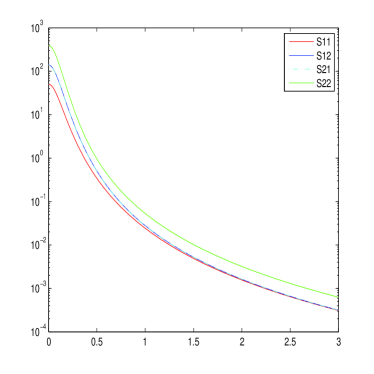
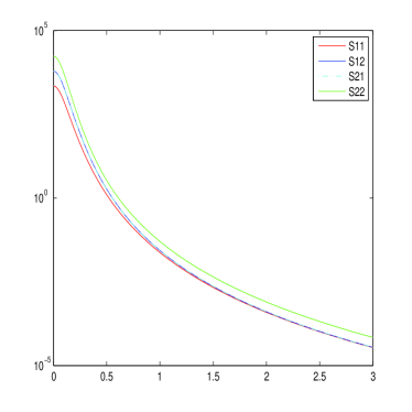
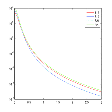
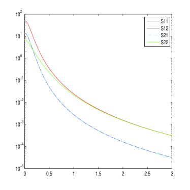
The asymptotic behavior of the power spectra for the bivariate GRF can be obtained from (54). For some selected parameter values defined in Table 1, the power spectra are shown in Figure 1. From these figure, we can notice that the parameters {bij;i,j=1,2,i>j}formulae-sequencesubscript𝑏𝑖𝑗𝑖𝑗12𝑖𝑗\{b_{ij};i,j=1,2,i>j\} controls the correlation between the two fields. When a smaller absolute value of b21subscript𝑏21b_{21} is chosen, the correlation between these two fields decreases rapidly. We can also show that the sign of b21b22subscript𝑏21subscript𝑏22b_{21}\cdot b_{22} is related the sign of the correlation between the two GRFs. Obviously, bijsubscript𝑏𝑖𝑗b_{ij} are also related to the variance of the GRFs. The parameters κijsubscript𝜅𝑖𝑗\kappa_{ij} are related to the range of the two fields. αijsubscript𝛼𝑖𝑗\alpha_{ij} and αnisubscript𝛼subscript𝑛𝑖\alpha_{n_{i}} are related to the smoothness of the two GRFs. The asymptotic behavior is curial when dealing with the real-world applications.

Table 1: Parameter values for asymptotic behaviors of the power spectra for bivariate GRFs
case 111 case 222
𝜶𝜶\boldsymbol{\alpha} 𝜿𝜿\boldsymbol{\kappa} 𝒃𝒃\boldsymbol{b} 𝜶𝜶\boldsymbol{\alpha} 𝜿𝜿\boldsymbol{\kappa} 𝒃𝒃\boldsymbol{b}
α11=2subscript𝛼112\alpha_{11}=2 κ11=0.15subscript𝜅110.15\kappa_{11}=0.15 b11=1subscript𝑏111b_{11}=1 α11=2subscript𝛼112\alpha_{11}=2 κ11=0.15subscript𝜅110.15\kappa_{11}=0.15 b11=1subscript𝑏111b_{11}=1
α12=0subscript𝛼120\alpha_{12}=0 κ12=0subscript𝜅120\kappa_{12}=0 b12=0subscript𝑏120b_{12}=0 α12=0subscript𝛼120\alpha_{12}=0 κ12=0subscript𝜅120\kappa_{12}=0 b12=0subscript𝑏120b_{12}=0
α21=2subscript𝛼212\alpha_{21}=2 κ21=0.5subscript𝜅210.5\kappa_{21}=0.5 b21=1subscript𝑏211b_{21}=-1 α21=2subscript𝛼212\alpha_{21}=2 κ21=0.5subscript𝜅210.5\kappa_{21}=0.5 b21=1subscript𝑏211b_{21}=-1
α22=2subscript𝛼222\alpha_{22}=2 κ22=0.3subscript𝜅220.3\kappa_{22}=0.3 b22=1subscript𝑏221b_{22}=1 α22=2subscript𝛼222\alpha_{22}=2 κ22=0.3subscript𝜅220.3\kappa_{22}=0.3 b22=1subscript𝑏221b_{22}=1
αn1=0subscript𝛼subscript𝑛10\alpha_{n_{1}}=0 κn1=0.15subscript𝜅subscript𝑛10.15\kappa_{n_{1}}=0.15 αn1=1subscript𝛼subscript𝑛11\alpha_{n_{1}}=1 κn1=0.15subscript𝜅subscript𝑛10.15\kappa_{n_{1}}=0.15
αn1=0subscript𝛼subscript𝑛10\alpha_{n_{1}}=0 κn2=0.3subscript𝜅subscript𝑛20.3\kappa_{n_{2}}=0.3 αn2=1subscript𝛼subscript𝑛21\alpha_{n_{2}}=1 κn2=0.3subscript𝜅subscript𝑛20.3\kappa_{n_{2}}=0.3
case 333 case 444
𝜶𝜶\boldsymbol{\alpha} 𝜿𝜿\boldsymbol{\kappa} 𝒃𝒃\boldsymbol{b} 𝜶𝜶\boldsymbol{\alpha} 𝜿𝜿\boldsymbol{\kappa} 𝒃𝒃\boldsymbol{b}
α11=2subscript𝛼112\alpha_{11}=2 κ11=0.15subscript𝜅110.15\kappa_{11}=0.15 b11=1subscript𝑏111b_{11}=1 α11=2subscript𝛼112\alpha_{11}=2 κ11=0.15subscript𝜅110.15\kappa_{11}=0.15 b11=1subscript𝑏111b_{11}=1
α12=0subscript𝛼120\alpha_{12}=0 κ12=0subscript𝜅120\kappa_{12}=0 b12=0subscript𝑏120b_{12}=0 α12=0subscript𝛼120\alpha_{12}=0 κ12=0subscript𝜅120\kappa_{12}=0 b12=0subscript𝑏120b_{12}=0
α21=2subscript𝛼212\alpha_{21}=2 κ21=0.15subscript𝜅210.15\kappa_{21}=0.15 b21=0.5subscript𝑏210.5b_{21}=-0.5 α21=2subscript𝛼212\alpha_{21}=2 κ21=0.5subscript𝜅210.5\kappa_{21}=0.5 b21=1subscript𝑏211b_{21}=-1
α22=2subscript𝛼222\alpha_{22}=2 κ22=0.3subscript𝜅220.3\kappa_{22}=0.3 b22=1subscript𝑏221b_{22}=1 α22=2subscript𝛼222\alpha_{22}=2 κ22=0.3subscript𝜅220.3\kappa_{22}=0.3 b22=1subscript𝑏221b_{22}=1
αn1=0subscript𝛼subscript𝑛10\alpha_{n_{1}}=0 κn1=0.15subscript𝜅subscript𝑛10.15\kappa_{n_{1}}=0.15 αn1=0subscript𝛼subscript𝑛10\alpha_{n_{1}}=0 κn1=0.15subscript𝜅subscript𝑛10.15\kappa_{n_{1}}=0.15
αn1=0subscript𝛼subscript𝑛10\alpha_{n_{1}}=0 κn2=0.3subscript𝜅subscript𝑛20.3\kappa_{n_{2}}=0.3 αn2=0subscript𝛼subscript𝑛20\alpha_{n_{2}}=0 κn2=0.3subscript𝜅subscript𝑛20.3\kappa_{n_{2}}=0.3
Refer to caption
Refer to caption
Refer to caption
Refer to caption
Figure 1: Asymptotic behaviors of the power spectra corresponding to case 111 (a), case 222 (b), case 333 (c) and case 444 (d) with parameter values given in Table 1.

3.2 Bivariate GRF with the covariance-based model

As presented by Gneiting et al. (2010), a multivariate GRFs can be constructed using a covariance-based model. In the bivariate setting, the matrix-valued covariance function for the bivariate GRF contains 444 elements and the corresponding power spectrum matrix becomes

𝑹(𝒌)=(Rx11(𝒌)Rx12(𝒌)Rx21(𝒌)Rx22(𝒌)).𝑹𝒌subscript𝑅subscript𝑥11𝒌subscript𝑅subscript𝑥12𝒌subscript𝑅subscript𝑥21𝒌subscript𝑅subscript𝑥22𝒌\displaystyle\ \boldsymbol{R}(\boldsymbol{k})=\left(\begin{array}[]{cc}R_{x_{11}}(\boldsymbol{k})&R_{x_{12}}(\boldsymbol{k})\\ R_{x_{21}}(\boldsymbol{k})&R_{x_{22}}(\boldsymbol{k})\end{array}\right). (57)

Applying integral given in Equation (22), together with the expression for the marginal variances in Equation (7) and cross-covariance in Equation (8), we can find closed form for the elements in the power spectrum matrix,

Rxii(𝒌)=1(2π)d[aii2νii(4π)dσiiΓ(νii+d/2)(aii2+𝒌2)νii+d/2Γ(νii)],Rxij(𝒌)=1(2π)d[aij2νij(4π)dρijσiσjΓ(νij+d/2)(aij2+𝒌2)νij+d/2Γ(νij)].formulae-sequencesubscript𝑅subscript𝑥𝑖𝑖𝒌1superscript2𝜋𝑑delimited-[]superscriptsubscript𝑎𝑖𝑖2subscript𝜈𝑖𝑖superscript4𝜋𝑑subscript𝜎𝑖𝑖Γsubscript𝜈𝑖𝑖𝑑2superscriptsuperscriptsubscript𝑎𝑖𝑖2superscriptnorm𝒌2subscript𝜈𝑖𝑖𝑑2Γsubscript𝜈𝑖𝑖subscript𝑅subscript𝑥𝑖𝑗𝒌1superscript2𝜋𝑑delimited-[]superscriptsubscript𝑎𝑖𝑗2subscript𝜈𝑖𝑗superscript4𝜋𝑑subscript𝜌𝑖𝑗subscript𝜎𝑖subscript𝜎𝑗Γsubscript𝜈𝑖𝑗𝑑2superscriptsuperscriptsubscript𝑎𝑖𝑗2superscriptnorm𝒌2subscript𝜈𝑖𝑗𝑑2Γsubscript𝜈𝑖𝑗\begin{split}R_{x_{ii}}(\boldsymbol{k})&=\frac{1}{(2\pi)^{d}}\left[a_{ii}^{2\nu_{ii}}(\sqrt{4\pi})^{d}\frac{\sigma_{ii}\Gamma(\nu_{ii}+d/2)}{(a_{ii}^{2}+\|\boldsymbol{k}\|^{2})^{\nu_{ii}+d/2}\Gamma(\nu_{ii})}\right],\\ R_{x_{ij}}(\boldsymbol{k})&=\frac{1}{(2\pi)^{d}}\left[a_{ij}^{2\nu_{ij}}(\sqrt{4\pi})^{d}\frac{\rho_{ij}\sigma_{i}\sigma_{j}\Gamma(\nu_{ij}+d/2)}{(a_{ij}^{2}+\|\boldsymbol{k}\|^{2})^{\nu_{ij}+d/2}\Gamma(\nu_{ij})}\right].\end{split} (58)

Notice that if d={2,4,}𝑑24d=\{2,4,...\}, then the expressions in (58) can be simplified even further by (recursively) using the well-known formula

Γ(ν+1)=νΓ(ν).Γ𝜈1𝜈Γ𝜈\Gamma(\nu+1)=\nu\Gamma(\nu).

Since all the components {Cij;i,j=1,2}formulae-sequencesubscript𝐶𝑖𝑗𝑖𝑗12\{C_{ij};i,j=1,2\} in the matrix-valued covariance matrix 𝑪𝑪\boldsymbol{C} are from Matérn family, as defined in Equation (7) and Equation (8) (Gneiting et al., 2010), the power spectra of the marginal covariance functions {Cii;i=1,2}formulae-sequencesubscript𝐶𝑖𝑖𝑖12\{C_{ii};i=1,2\} and the cross covariance functions {Cij;i,j=1,2,ij}formulae-sequencesubscript𝐶𝑖𝑗𝑖𝑗12𝑖𝑗\{C_{ij};i,j=1,2,i\neq j\} have similar forms as indicated in (58).

3.3 Parameter matching

As mentioned in Section 2.2, the model comparison in this paper is based on the fact that if Sij(𝒌)=Rij(𝒌)subscript𝑆𝑖𝑗𝒌subscript𝑅𝑖𝑗𝒌S_{ij}(\boldsymbol{k})=R_{ij}(\boldsymbol{k}), for each 1i,jpformulae-sequence1𝑖𝑗𝑝1\leq i,j\leq p, and then the multivariate GRFs constructed from the SPDEs approach (12) and from the covariance-based model (6) will be equivalent.

By comparing each element in (54) and (58), we can get the results given as follows,

0=ρ12ρ21,κ11=κ21=κ22=κn1=κn2=a11=a12=a21=a22,α11+αn1=ν11+d2,α11+α222+αn1α212=ν12+d2,formulae-sequenceformulae-sequence0subscript𝜌12subscript𝜌21subscript𝜅11subscript𝜅21subscript𝜅22subscript𝜅subscript𝑛1subscript𝜅subscript𝑛2subscript𝑎11subscript𝑎12subscript𝑎21subscript𝑎22formulae-sequencesubscript𝛼11subscript𝛼subscript𝑛1subscript𝜈11𝑑2subscript𝛼11subscript𝛼222subscript𝛼subscript𝑛1subscript𝛼212subscript𝜈12𝑑2\begin{split}0&=\rho_{12}-\rho_{21},\\ \kappa_{11}=\kappa_{21}=\kappa_{22}=\kappa_{n_{1}}=\kappa_{n_{2}}&=a_{11}=a_{12}=a_{21}=a_{22},\\ \alpha_{11}+\alpha_{n_{1}}&=\nu_{11}+\frac{d}{2},\\ \alpha_{11}+\frac{\alpha_{22}}{2}+\alpha_{n_{1}}-\frac{\alpha_{21}}{2}&=\nu_{12}+\frac{d}{2},\\ \end{split} (59)

and

1b112=(4π)d/2a112νn1σ11Γ(ν11+d/2)Γ(ν11),b21b22b112=(4π)d/2a122ν12Γ(ν12+d/2)ρ12σ1σ2Γ(ν12),b212+b112b112b222=(4π)d/2σ22a222ν22Γ(ν22+d/2)Γ(ν22).formulae-sequence1superscriptsubscript𝑏112superscript4𝜋𝑑2superscriptsubscript𝑎112subscript𝜈𝑛1subscript𝜎11Γsubscript𝜈11𝑑2Γsubscript𝜈11formulae-sequencesubscript𝑏21subscript𝑏22superscriptsubscript𝑏112superscript4𝜋𝑑2superscriptsubscript𝑎122subscript𝜈12Γsubscript𝜈12𝑑2subscript𝜌12subscript𝜎1subscript𝜎2Γsubscript𝜈12superscriptsubscript𝑏212superscriptsubscript𝑏112superscriptsubscript𝑏112superscriptsubscript𝑏222superscript4𝜋𝑑2subscript𝜎22superscriptsubscript𝑎222subscript𝜈22Γsubscript𝜈22𝑑2Γsubscript𝜈22\begin{split}&\frac{1}{b_{11}^{2}}=\frac{(4\pi)^{d/2}a_{11}^{2\nu_{n1}}\sigma_{11}\Gamma(\nu_{11}+d/2)}{\Gamma(\nu_{11})},\\ &-\frac{b_{21}}{b_{22}b_{11}^{2}}=\frac{(4\pi)^{d/2}a_{12}^{2\nu_{12}}\Gamma(\nu_{12}+d/2)\rho_{12}\sigma_{1}\sigma_{2}}{\Gamma(\nu_{12})},\\ &\frac{b_{21}^{2}+b_{11}^{2}}{b_{11}^{2}b_{22}^{2}}=\frac{(4\pi)^{d/2}\sigma_{22}a_{22}^{2\nu_{22}}\Gamma(\nu_{22}+d/2)}{\Gamma(\nu_{22})}.\end{split} (60)

More equalities can be obtained based on the relationship between α21+αn2subscript𝛼21subscript𝛼subscript𝑛2\alpha_{21}+\alpha_{n_{2}} and α11+αn1subscript𝛼11subscript𝛼subscript𝑛1\alpha_{11}+\alpha_{n_{1}}. When α21+αn2α11+αn1subscript𝛼21subscript𝛼subscript𝑛2subscript𝛼11subscript𝛼subscript𝑛1\alpha_{21}+\alpha_{n_{2}}\leq\alpha_{11}+\alpha_{n_{1}}, we can get

αn2+α22=ν22+d2.subscript𝛼subscript𝑛2subscript𝛼22subscript𝜈22𝑑2\alpha_{n_{2}}+\alpha_{22}=\nu_{22}+\frac{d}{2}. (61)

When α21+αn2α11+αn1subscript𝛼21subscript𝛼subscript𝑛2subscript𝛼11subscript𝛼subscript𝑛1\alpha_{21}+\alpha_{n_{2}}\geq\alpha_{11}+\alpha_{n_{1}}, we can get

α11+α22+αn1α21=ν22+d2.subscript𝛼11subscript𝛼22subscript𝛼subscript𝑛1subscript𝛼21subscript𝜈22𝑑2\begin{split}\alpha_{11}+\alpha_{22}+\alpha_{n_{1}}-\alpha_{21}=\nu_{22}+\frac{d}{2}.\end{split} (62)

The Equation (61) and Equation (62) are critical when discussing about the asymptotic behaviors of bivariate GRF and the corresponding power spectra. From (59), we can notice that in order to construct equivalent models to the ones as discussed by Gneiting et al. (2010), we need to have the constraint that all the scaling parameters should be equal in addition to some constraints for the smoothness parameters given in the third and the fourth equations in (59) and one more conditional equality given in (61) or (62). From the first equation in (59), we notice the extra symmetry restriction discussed in Gneiting et al. (2010, Section 444) also must be fulfilled. Additionally, from the second equation in (60), we notice that there is one important relationship

ρ12b22b210,subscript𝜌12subscript𝑏22subscript𝑏210\begin{split}\rho_{12}b_{22}b_{21}&\leq 0,\end{split} (63)

between the co-located correlation coefficient ρ12subscript𝜌12\rho_{12} and b21subscript𝑏21b_{21} and b22subscript𝑏22b_{22}. It shows that the correlation ρ12subscript𝜌12\rho_{12} must have opposite sign to the product of b21subscript𝑏21b_{21} and b22subscript𝑏22b_{22}. This is an important information not only for sampling from the bivariate GRFs but also for interpreting the results from inference.

From the results given in (60), we can obtain the following results

b22b21=a11ν11σ1Γ(ν11+d/2)/Γ(ν11)a12ν12ρσ2Γ(ν12+d/2)/Γ(ν12),b222b112+b212=a11ν11σ11Γ(ν11+d/2)/Γ(ν11)a22ν22σ22Γ(ν22+d/2)/Γ(ν22).formulae-sequencesubscript𝑏22subscript𝑏21superscriptsubscript𝑎11subscript𝜈11subscript𝜎1Γsubscript𝜈11𝑑2Γsubscript𝜈11superscriptsubscript𝑎12subscript𝜈12𝜌subscript𝜎2Γsubscript𝜈12𝑑2Γsubscript𝜈12superscriptsubscript𝑏222superscriptsubscript𝑏112superscriptsubscript𝑏212superscriptsubscript𝑎11subscript𝜈11subscript𝜎11Γsubscript𝜈11𝑑2Γsubscript𝜈11superscriptsubscript𝑎22subscript𝜈22subscript𝜎22Γsubscript𝜈22𝑑2Γsubscript𝜈22\begin{split}-\frac{b_{22}}{b_{21}}&=\frac{a_{11}^{\nu_{11}}\sigma_{1}\Gamma({\nu_{11}+d/2})/\Gamma({\nu_{11}})}{a_{12}^{\nu_{12}}\rho\sigma_{2}\Gamma({\nu_{12}+d/2})/\Gamma({\nu_{12}})},\\ \frac{b_{22}^{2}}{b_{11}^{2}+b_{21}^{2}}&=\frac{a_{11}^{\nu_{11}}\sigma_{11}\Gamma({\nu_{11}+d/2})/\Gamma({\nu_{11}})}{a_{22}^{\nu_{22}}\sigma_{22}\Gamma({\nu_{22}+d/2})/\Gamma({\nu_{22}})}.\end{split} (64)

Notice that when a11=a21=a22subscript𝑎11subscript𝑎21subscript𝑎22a_{11}=a_{21}=a_{22} and ν11=ν21=ν22subscript𝜈11subscript𝜈21subscript𝜈22\nu_{11}=\nu_{21}=\nu_{22}, the above results in (64) can be simplified to the following form

b22b21=σ1ρσ2,b222b112+b212=σ11σ22.formulae-sequencesubscript𝑏22subscript𝑏21subscript𝜎1𝜌subscript𝜎2superscriptsubscript𝑏222superscriptsubscript𝑏112superscriptsubscript𝑏212subscript𝜎11subscript𝜎22\begin{split}-\frac{b_{22}}{b_{21}}&=\frac{\sigma_{1}}{\rho\sigma_{2}},\\ \frac{b_{22}^{2}}{b_{11}^{2}+b_{21}^{2}}&=\frac{\sigma_{11}}{\sigma_{22}}.\end{split} (65)

These results show that the parameters {bij;i,j=1,2}formulae-sequencesubscript𝑏𝑖𝑗𝑖𝑗12\{b_{ij};i,j=1,2\} are not only connected to the correlation between these two fields, but also connected with the marginal variance of the GRF. From the results given in (59) to (65), we can notice that the parameters in the system of SPDEs have similar interpretations as the parameters from the covariance-based model.

From these results we see that it is possible to construct multivariate GRFs through the SPDEs approach as the covariance-based approach proposed by Gneiting et al. (2010). Additionally, there are three main advantages for our SPDEs approach. The first advantage is that our new approach does not explicitly depend on the theory of positive definite matrix. We do not need to worry about the notorious requirement of positive definite covariance matrices. The second advantage is that we can remove the symmetry property which is shared by the covariance-based approach and the LMC approach (Gelfand et al., 2004; Gneiting et al., 2010). The third advantage, which has not yet been discussed, is that we can construct multivariate GRFs on manifolds, such as the sphere 𝕊2superscript𝕊2\mathbb{S}^{2}, by simply reinterpret the systems of SPDEs to be defined on the manifold. Lindgren et al. (2011, Section 3.13.13.1) discussed the theoretical background in the univariate setting, which is basically the same as for our multivariate setting.

Furthermore, we can actually go even future for the multivariate GRFs, such as multivariate GRFs with oscillating covariance functions and non-stationary multivariate GRFs. These kinds of multivariate GRFs are under development but are beyond the scope of this paper.

3.4 Sampling bivariate GRFs and trivariate GRFs

As presented in Section 2.3 we can construct multivariate GRFs by the SPDEs approach theoretically, but do the computations using the GMRF representation. The precision matrix 𝑸𝑸\boldsymbol{Q} is usually sparse and the sparseness of the precision matrices enables us to apply numerical linear algebra for sparse matrices for sampling from the GRFs and for fast statistical inference. We now assume that the multivariate GMRF has mean vector 𝝁𝝁\boldsymbol{\mu} and precision matrix 𝑸𝑸\boldsymbol{Q}, i.e., 𝒙𝒩(𝝁,𝑸1)similar-to𝒙𝒩𝝁superscript𝑸1\boldsymbol{x}\sim\mathcal{N}(\boldsymbol{\mu},\boldsymbol{Q}^{-1}). When sampling from the GMRF, the forward substitution and backward substitution is applied by using the Cholesky triangle 𝑳𝑳\boldsymbol{L}, where by definition 𝑸=𝑳𝑳T𝑸𝑳superscript𝑳T\boldsymbol{Q}=\boldsymbol{L}\boldsymbol{L}^{\text{T}}. The commonly used steps for sampling a GRF are as follows.

  1. 1.

    Calculate the Cholesky triangle 𝑳𝑳\boldsymbol{L} from the Cholesky factorization;

  2. 2.

    Sample 𝒛𝒩(𝟎,𝑰)similar-to𝒛𝒩0𝑰\boldsymbol{z}\sim\mathcal{N}(\boldsymbol{0},\boldsymbol{I}), where 𝑰𝑰\boldsymbol{I} is the identity matrix with the same dimensions as the precision matrix 𝑸𝑸\boldsymbol{Q};

  3. 3.

    Solve the linear system of equations 𝑳𝒗=𝒛𝑳𝒗𝒛\boldsymbol{L}\boldsymbol{v}=\boldsymbol{z} for 𝒗𝒗\boldsymbol{v}. Then 𝒗𝒗\boldsymbol{v} has the correct precision matrix 𝑸𝑸\boldsymbol{Q}, and 𝒗𝒩(𝟎,𝑸1)similar-to𝒗𝒩0superscript𝑸1\boldsymbol{v}\sim\mathcal{N}(\boldsymbol{0},\boldsymbol{Q}^{-1});

  4. 4.

    Finally correct the mean by computing 𝒙=𝝁+𝒗𝒙𝝁𝒗\boldsymbol{x}=\boldsymbol{\mu}+\boldsymbol{v}.

Then 𝒙𝒙\boldsymbol{x} is a sample of the GMRF with correct mean 𝝁𝝁\boldsymbol{\mu} and precision matrix 𝑸𝑸\boldsymbol{Q}. If 𝑸𝑸\boldsymbol{Q} is a band matrix, a band-Cholesky factorization can be used with the algorithm given by Rue and Held (2005, Algorithm 2.92.92.9, Page 454545). Different types of parametrization of GMRFs and their corresponding sampling procedures can be found in Rue and Held (2005). If the mean of the field is 𝟎0\boldsymbol{0}, the Step 444 is not needed and 𝒗𝒗\boldsymbol{v} is a sample from the GMRF.

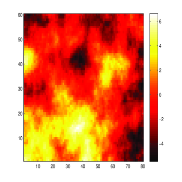
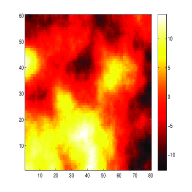
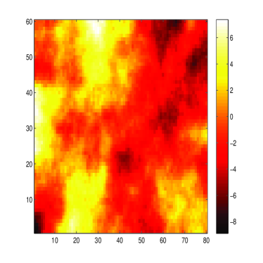
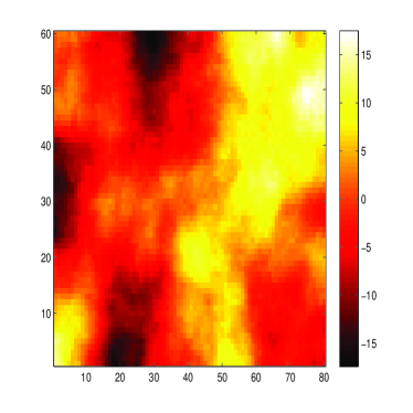
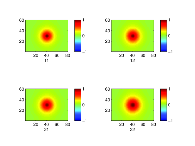
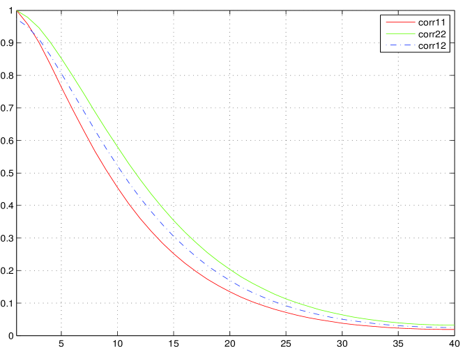
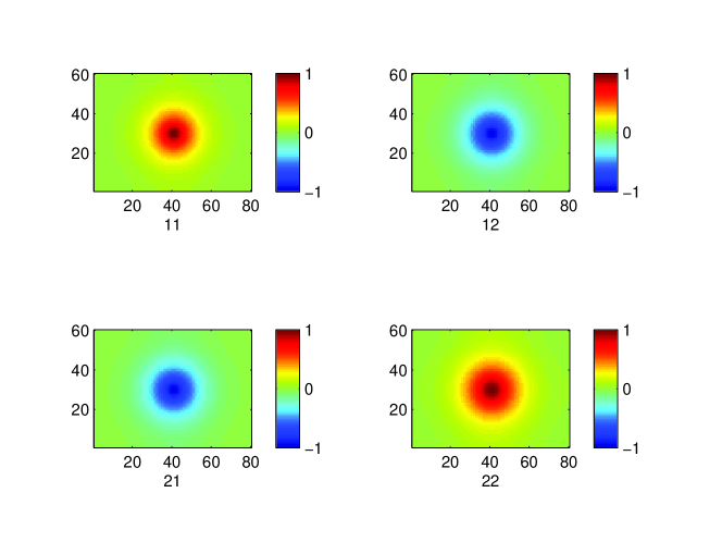
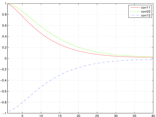
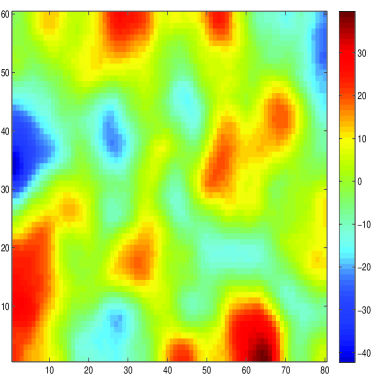
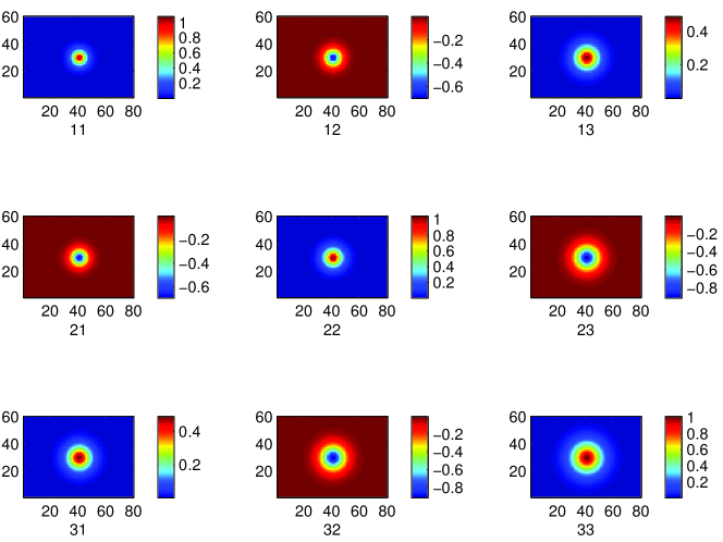
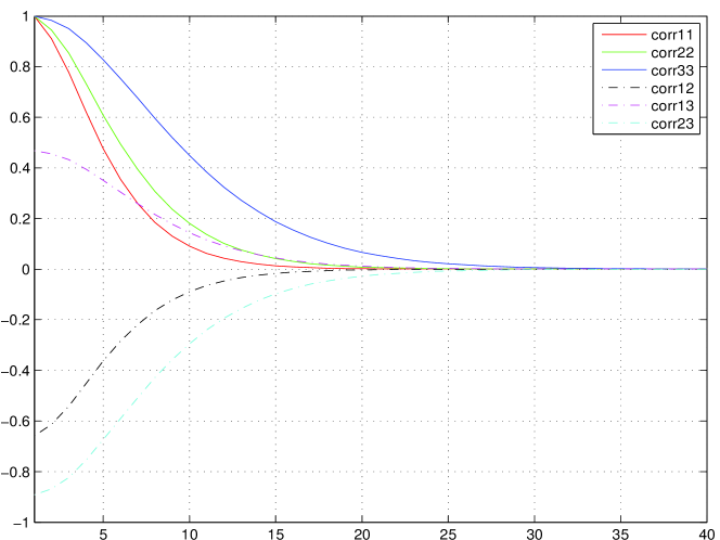
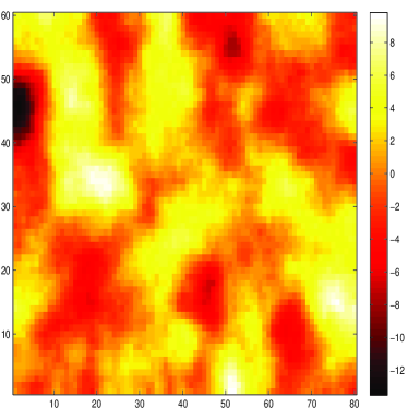
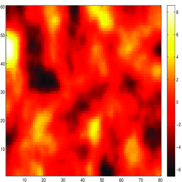
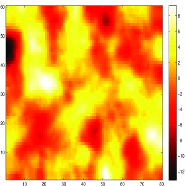
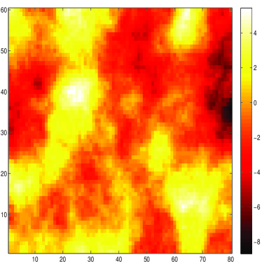
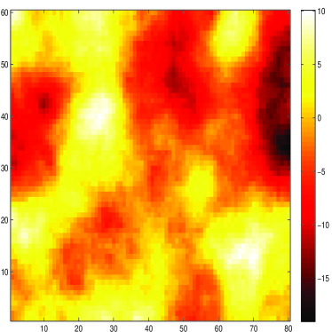
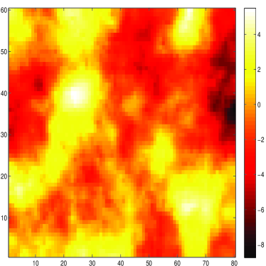
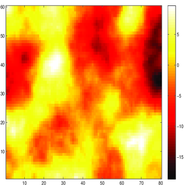
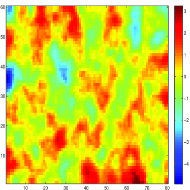
With white noise at the right hand of SPDEs (40), and the parameters from the differential operators given in Table 2, we can get samples for positively correlated random fields with b21<0subscript𝑏210b_{21}<0 and negatively correlated random fields with b21>0subscript𝑏210b_{21}>0. These two samples are shown in Figure 2 and Figure 3. Choosing the reference points in the middle of the two GRFs for these two cases, we can get the corresponding marginal correlations within each of the GRFs and the cross-correlations between the two GRFs. The results are shown in Figure 4 and Figure 6. We can see that the random fields are isotropic and have the same correlation range. This is because we have chosen almost the same parameters for our cases, except the signs of b21subscript𝑏21b_{21}.

Table 2: Parameters for sampling bivariate GRFs
positively correlated GRFs negatively correlated GRFs
𝜶𝜶\boldsymbol{\alpha} 𝜿𝜿\boldsymbol{\kappa} 𝒃𝒃\boldsymbol{b} 𝜶𝜶\boldsymbol{\alpha} 𝜿𝜿\boldsymbol{\kappa} 𝒃𝒃\boldsymbol{b}
α11=2subscript𝛼112\alpha_{11}=2 κ11=0.15subscript𝜅110.15\kappa_{11}=0.15 b11=1subscript𝑏111b_{11}=1 α11=2subscript𝛼112\alpha_{11}=2 κ11=0.15subscript𝜅110.15\kappa_{11}=0.15 b11=1subscript𝑏111b_{11}=1
α12=0subscript𝛼120\alpha_{12}=0 κ12=0subscript𝜅120\kappa_{12}=0 b12=0subscript𝑏120b_{12}=0 α12=0subscript𝛼120\alpha_{12}=0 κ12=0subscript𝜅120\kappa_{12}=0 b12=0subscript𝑏120b_{12}=0
α21=2subscript𝛼212\alpha_{21}=2 κ21=0.5subscript𝜅210.5\kappa_{21}=0.5 b21=1subscript𝑏211b_{21}=-1 α21=2subscript𝛼212\alpha_{21}=2 κ21=0.5subscript𝜅210.5\kappa_{21}=0.5 b21=1subscript𝑏211b_{21}=1
α22=2subscript𝛼222\alpha_{22}=2 κ22=0.3subscript𝜅220.3\kappa_{22}=0.3 b22=1subscript𝑏221b_{22}=1 α22=2subscript𝛼222\alpha_{22}=2 κ22=0.3subscript𝜅220.3\kappa_{22}=0.3 b22=1subscript𝑏221b_{22}=1
αn1=0subscript𝛼subscript𝑛10\alpha_{n_{1}}=0 κn1=0.15subscript𝜅subscript𝑛10.15\kappa_{n_{1}}=0.15 αn1=0subscript𝛼subscript𝑛10\alpha_{n_{1}}=0 κn1=0.15subscript𝜅subscript𝑛10.15\kappa_{n_{1}}=0.15
αn2=0subscript𝛼subscript𝑛20\alpha_{n_{2}}=0 κn2=0.3subscript𝜅subscript𝑛20.3\kappa_{n_{2}}=0.3 αn2=0subscript𝛼subscript𝑛20\alpha_{n_{2}}=0 κn2=0.3subscript𝜅subscript𝑛20.3\kappa_{n_{2}}=0.3
Refer to caption
Refer to caption
Figure 2: One simulated realization from the bivariate Gaussian Random Field with positive correlation with parameters α11=2,α12=0,α21=2,α22=2,αn1=0,αn2=0formulae-sequencesubscript𝛼112formulae-sequencesubscript𝛼120formulae-sequencesubscript𝛼212formulae-sequencesubscript𝛼222formulae-sequencesubscript𝛼subscript𝑛10subscript𝛼subscript𝑛20\alpha_{11}=2,\alpha_{12}=0,\alpha_{21}=2,\alpha_{22}=2,\alpha_{n_{1}}=0,\alpha_{n_{2}}=0, κ11=0.15,κ22=0.3,κ21=0.5,κn1=0.15,κn2=0.3formulae-sequencesubscript𝜅110.15formulae-sequencesubscript𝜅220.3formulae-sequencesubscript𝜅210.5formulae-sequencesubscript𝜅subscript𝑛10.15subscript𝜅subscript𝑛20.3\kappa_{11}=0.15,\kappa_{22}=0.3,\kappa_{21}=0.5,\kappa_{n_{1}}=0.15,\kappa_{n_{2}}=0.3, b11=1,b12=0,b22=1formulae-sequencesubscript𝑏111formulae-sequencesubscript𝑏120subscript𝑏221b_{11}=1,b_{12}=0,b_{22}=1 and b21=1subscript𝑏211b_{21}=-1.
Refer to caption
Refer to caption
Figure 3: One simulated realization from the bivariate Gaussian Random Field with negative correlation with parameters α11=2,α12=0,α21=2,α22=2,αn1=0,αn2=0formulae-sequencesubscript𝛼112formulae-sequencesubscript𝛼120formulae-sequencesubscript𝛼212formulae-sequencesubscript𝛼222formulae-sequencesubscript𝛼subscript𝑛10subscript𝛼subscript𝑛20\alpha_{11}=2,\alpha_{12}=0,\alpha_{21}=2,\alpha_{22}=2,\alpha_{n_{1}}=0,\alpha_{n_{2}}=0, κ11=0.15,κ22=0.3,κ21=0.5,κn1=0.15,κn2=0.3formulae-sequencesubscript𝜅110.15formulae-sequencesubscript𝜅220.3formulae-sequencesubscript𝜅210.5formulae-sequencesubscript𝜅subscript𝑛10.15subscript𝜅subscript𝑛20.3\kappa_{11}=0.15,\kappa_{22}=0.3,\kappa_{21}=0.5,\kappa_{n_{1}}=0.15,\kappa_{n_{2}}=0.3, b11=1,b12=0,b22=1formulae-sequencesubscript𝑏111formulae-sequencesubscript𝑏120subscript𝑏221b_{11}=1,b_{12}=0,b_{22}=1 and b21=1subscript𝑏211b_{21}=1.
Refer to caption
Figure 4: Marginal correlations (diagonal direction) and cross-correlations (anti-diagonal direction) with the reference points in the middle of the two GRFs for the positively correlated random fields.
Refer to caption
Figure 5: Marginal correlations and cross-correlations with the reference points in the middle of the two GRFs for the positively correlated random fields. ’corr11’ means the marginal correlation within random field 111. ’corr22’ means the marginal correlation within random field 222. ’corr12’ means the cross-correlation between random fields 111 and 222.
Refer to caption
Figure 6: Marginal correlations (diagonal direction) and cross-correlations (anti-diagonal direction) with the reference points in the middle of the two GRFs for the negatively correlated random fields.
Refer to caption
Figure 7: Marginal correlations and cross-correlations with the reference points in the middle of the two GRFs for the negatively correlated random fields. ’corr11’ means the marginal correlation within random field 111. ’corr22’ means the marginal correlation within random field 222. ’corr12’ means the cross-correlation between random fields 111 and 222.

From Figure 2 - Figure 6 and many more samples from the bivariate GRFs which we have simulated, we can notice that the sign of b21b22subscript𝑏21subscript𝑏22b_{21}\cdot b_{22} is related to the sign of the correlation between these two GRFs, which corresponds to the comparison result in (63). The smoothness of the GRFs are related to the values αijsubscript𝛼𝑖𝑗\alpha_{ij}. These results also verify the conclusion given in (59).

We can also notice that the first GRF is a Matérn random field when we use the white noise process as the driving process or under the condition that κn1=κ11subscript𝜅subscript𝑛1subscript𝜅11\kappa_{n_{1}}=\kappa_{11} with the triangular systems of SPDEs. The second field, in general, is not a Matérn random field, but it can be relatively close to a Matérn random field. With additional conditions, the second random fields could also be a Matérn random field, but this is not focused in this paper. With the triangular system of SPDEs, together with some other conditions, the correlation range which was mentioned in Section 1 for the first random field can be calculated by the empirically derived formula ρ=8ν/κ𝜌8𝜈𝜅\rho=\sqrt{8\nu}/\kappa but not for the second random field. In general we need to find the correlation ranges for the random fields numerically.

For trivariate GRFs the sampling procedure is exactly the same as for bivariate GRFs. We use the triangular system of the SPDEs. The true values given in Table 7 are used. One sample from the trivariate GRFs is shown in Figure 8 with the corresponding correlation functions given in Figure 9. From these figures, we notice that the trivariate random fields have similar interpretation as the bivariate random fields, but are more complicated. Since the triangular version of the system of SPDEs has been used, the sign of b21b22subscript𝑏21subscript𝑏22b_{21}\cdot b_{22} is related to the sign of the correlation between the first two GRFs. But for the third fields, it is not only related to the sign of b32b33subscript𝑏32subscript𝑏33b_{32}\cdot b_{33} but also the influence from the sign of b21b22subscript𝑏21subscript𝑏22b_{21}\cdot b_{22}. By choosing a different parametrization, we can end up with more interesting models such as the random field 111 and random field 333 are positively correlated in some locations and negatively correlated in other locations. We are not going to discuss these issues here since this is ongoing research.
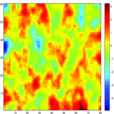
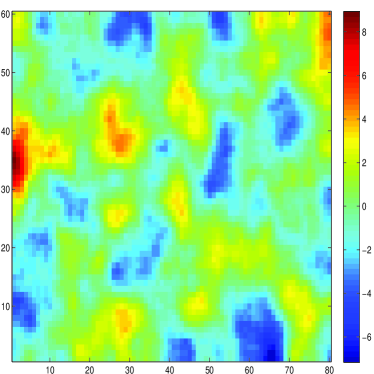
Table 3: Parameters for sampling trivariate GRFs
𝜶𝜶\boldsymbol{\alpha} 𝜿𝜿\boldsymbol{\kappa} 𝒃𝒃\boldsymbol{b}
α11=2subscript𝛼112\alpha_{11}=2 κ11=0.5subscript𝜅110.5\kappa_{11}=0.5 b11=1subscript𝑏111b_{11}=1
α12=0subscript𝛼120\alpha_{12}=0 κ12=0subscript𝜅120\kappa_{12}=0 b12=0subscript𝑏120b_{12}=0
α13=0subscript𝛼130\alpha_{13}=0 κ13=0subscript𝜅130\kappa_{13}=0 b13=0subscript𝑏130b_{13}=0
α21=2subscript𝛼212\alpha_{21}=2 κ21=0.6subscript𝜅210.6\kappa_{21}=0.6 b21=0.8subscript𝑏210.8b_{21}=0.8
α22=2subscript𝛼222\alpha_{22}=2 κ22=0.4subscript𝜅220.4\kappa_{22}=0.4 b22=1subscript𝑏221b_{22}=1
α23=0subscript𝛼230\alpha_{23}=0 κ23=0subscript𝜅230\kappa_{23}=0 b23=0subscript𝑏230b_{23}=0
α31=2subscript𝛼312\alpha_{31}=2 κ31=0.5subscript𝜅310.5\kappa_{31}=0.5 b31=1subscript𝑏311b_{31}=1
α32=2subscript𝛼322\alpha_{32}=2 κ32=1subscript𝜅321\kappa_{32}=1 b32=0.9subscript𝑏320.9b_{32}=0.9
α33=2subscript𝛼332\alpha_{33}=2 κ33=0.3subscript𝜅330.3\kappa_{33}=0.3 b33=1subscript𝑏331b_{33}=1
αn1=1subscript𝛼subscript𝑛11\alpha_{n_{1}}=1 κn1=0.5subscript𝜅subscript𝑛10.5\kappa_{n_{1}}=0.5
αn2=1subscript𝛼subscript𝑛21\alpha_{n_{2}}=1 κn2=0.4subscript𝜅subscript𝑛20.4\kappa_{n_{2}}=0.4
αn3=1subscript𝛼subscript𝑛31\alpha_{n_{3}}=1 κn3=0.3subscript𝜅subscript𝑛30.3\kappa_{n_{3}}=0.3
Refer to caption
Refer to caption
Refer to caption
Figure 8: One simulated realization from the trivariate Gaussian Random Fields with parameters given in Table 3.
Refer to caption
Figure 9: Marginal correlation matrices (diagonal) and cross-correlation matrices (off-diagonal) with each of the reference point in the middle of the three GRFs.
Refer to caption
Figure 10: Marginal correlation matrices and cross-correlation matrices with each of the reference point in the middle of the three GRFs. ’corr11’ means the marginal correlation within random field 111. ’corr22’ means the marginal correlation within random field 222. ’corr33’ means the marginal correlation within random field 333. ’corr12’ means the cross-correlation between random fields 111 and 222. ’corr13’ means the cross-correlation between random fields 111 and 333. ’corr23’ means the cross-correlation between random fields 222 and 333.

4 Examples and applications

In order to illustrate how to use the SPDEs approach for constructing multivariate GRFs and the usefulness of our approach, some examples both with simulated data and real data are chosen. First, some basic theory on inference with multivariate GMRFs is given. We focus on the triangular system of SPDEs in this paper.

We use the bivariate GMRFs as an example. The multivariate GMRFs can be done analogously. Assume that we have used N𝑁N triangles in the discretization for each random field xi(𝒔)|θi,i=1,2conditionalsubscript𝑥𝑖𝒔subscript𝜃𝑖𝑖12x_{i}(\boldsymbol{s})|\theta_{i},i=1,2. For the bivariate case 𝒙(𝒔)=(x(𝒔)1,x(𝒔)2)T𝒙𝒔superscript𝑥subscript𝒔1𝑥subscript𝒔2T\boldsymbol{x}(\boldsymbol{s})=\left(x(\boldsymbol{s})_{1},x(\boldsymbol{s})_{2}\right)^{\text{T}} has a 2N2𝑁2N-dimensional multivariate Gaussian distribution with probability density function

π(𝒙|𝜽)=(12π)2N|𝑸(𝜽)|1/2exp(12𝒙T𝑸(𝜽)𝒙),𝜋conditional𝒙𝜽superscript12𝜋2𝑁superscript𝑸𝜽1212superscript𝒙T𝑸𝜽𝒙\pi(\boldsymbol{x}|\boldsymbol{\theta})=\left(\frac{1}{2\pi}\right)^{2N}|\boldsymbol{Q}(\boldsymbol{\theta})|^{1/2}\exp\left(-\frac{1}{2}\boldsymbol{x}^{\text{T}}\boldsymbol{Q}(\boldsymbol{\theta})\boldsymbol{x}\right), (66)

where 𝑸(𝜽)𝑸𝜽\boldsymbol{Q}(\boldsymbol{\theta}) is the precision matrix of the bivariate GMRF with the parameters 𝜽𝜽\boldsymbol{\theta}. Furthermore, we assume the length of the data 𝒚=(y1,y2)T𝒚superscriptsubscript𝑦1subscript𝑦2T\boldsymbol{y}=(y_{1},y_{2})^{\text{T}} is t=k1+k2𝑡subscript𝑘1subscript𝑘2t=k_{1}+k_{2} where y1subscript𝑦1y_{1} is the observation of x1(𝒔)subscript𝑥1𝒔x_{1}(\boldsymbol{s}) with length k1subscript𝑘1k_{1} and y2subscript𝑦2y_{2} is the observation of x2(𝒔)subscript𝑥2𝒔x_{2}(\boldsymbol{s}) with length k2subscript𝑘2k_{2}. Then 𝒚𝒚\boldsymbol{y} is a t𝑡t-dimensional random variable with probability density function

π(𝒚|𝒙,𝜽)=(12π)t|𝑸n|1/2exp(12(𝒚𝑨𝒙)T𝑸n(𝒚𝑨𝒙)),𝜋conditional𝒚𝒙𝜽superscript12𝜋𝑡superscriptsubscript𝑸𝑛1212superscript𝒚𝑨𝒙Tsubscript𝑸𝑛𝒚𝑨𝒙\pi(\boldsymbol{y|\boldsymbol{x},\boldsymbol{\theta}})=\left(\frac{1}{2\pi}\right)^{t}|\boldsymbol{Q}_{n}|^{1/2}\exp\left(-\frac{1}{2}(\boldsymbol{y}-\boldsymbol{Ax})^{\text{T}}\boldsymbol{Q}_{n}(\boldsymbol{y}-\boldsymbol{Ax})\right), (67)

where 𝑸nsubscript𝑸𝑛\boldsymbol{Q}_{n} is defined in Section 2.3 with size t×t𝑡𝑡t\times t, and 𝑨𝑨\boldsymbol{A} is a t×2N𝑡2𝑁t\times 2N matrix which links the sparse observations to our bivariate GMRFs. Notice that the density function π(𝒚|𝒙,𝜽)𝜋conditional𝒚𝒙𝜽\pi(\boldsymbol{y}|\boldsymbol{x},\boldsymbol{\theta}) is independent of 𝜽𝜽\boldsymbol{\theta}. Hence we can write the probability density function as π(𝒚|𝒙)𝜋conditional𝒚𝒙\pi(\boldsymbol{y}|\boldsymbol{x}). We first find the probability density function of 𝒙|𝒚,𝜽conditional𝒙𝒚𝜽{\boldsymbol{x}|\boldsymbol{y},\boldsymbol{\theta}} from (66) - (67)

π(𝒙|𝒚,𝜽)π(𝒙,𝒚|𝜽)=π(𝒙|𝜽)π(𝒚|𝒙,𝜽)exp(12(xT(𝑸(𝜽)+𝑨T𝑸n𝑨)𝒙2𝒙T𝑨T𝑸n𝒚)).proportional-to𝜋conditional𝒙𝒚𝜽𝜋𝒙conditional𝒚𝜽𝜋conditional𝒙𝜽𝜋conditional𝒚𝒙𝜽proportional-to12superscript𝑥T𝑸𝜽superscript𝑨Tsubscript𝑸𝑛𝑨𝒙2superscript𝒙Tsuperscript𝑨Tsubscript𝑸𝑛𝒚\begin{split}\pi(\boldsymbol{x}|\boldsymbol{y},\boldsymbol{\theta})&\propto\pi({\boldsymbol{x},\boldsymbol{y}|\boldsymbol{\theta}})\\ &=\pi(\boldsymbol{x}|\boldsymbol{\theta})\pi(\boldsymbol{y}|\boldsymbol{x},\boldsymbol{\theta})\\ &\propto\exp\left(-\frac{1}{2}\left(x^{\text{T}}(\boldsymbol{Q}(\boldsymbol{\theta})+\boldsymbol{A}^{\text{T}}\boldsymbol{Q}_{n}\boldsymbol{A})\boldsymbol{x}-2\boldsymbol{x}^{\text{T}}\boldsymbol{A}^{\text{T}}\boldsymbol{Q}_{n}\boldsymbol{y}\right)\right).\end{split} (68)

Let 𝝁c(𝜽)=𝑸c1(𝜽)𝑨T𝑸n𝒚subscript𝝁𝑐𝜽superscriptsubscript𝑸𝑐1𝜽superscript𝑨Tsubscript𝑸𝑛𝒚\boldsymbol{\mu}_{c}(\boldsymbol{\theta})=\boldsymbol{Q}_{c}^{-1}(\boldsymbol{\theta})\boldsymbol{A}^{\text{T}}\boldsymbol{Q}_{n}\boldsymbol{y}, and 𝑸c(𝜽)=𝑸(𝜽)+𝑨T𝑸n𝑨subscript𝑸𝑐𝜽𝑸𝜽superscript𝑨Tsubscript𝑸𝑛𝑨\boldsymbol{Q}_{c}(\boldsymbol{\theta})=\boldsymbol{Q}(\boldsymbol{\theta})+\boldsymbol{A}^{\text{T}}\boldsymbol{Q}_{n}\boldsymbol{A}, and then π(𝒙|𝒚,𝜽)𝜋conditional𝒙𝒚𝜽\pi(\boldsymbol{x}|\boldsymbol{y},\boldsymbol{\theta}) can be denoted as

𝒙|𝒚,𝜽𝒩(𝝁c(𝜽),𝑸c1(𝜽)),similar-toconditional𝒙𝒚𝜽𝒩subscript𝝁𝑐𝜽superscriptsubscript𝑸𝑐1𝜽{\boldsymbol{x}|\boldsymbol{y},\boldsymbol{\theta}}\sim\mathcal{N}\left(\boldsymbol{\mu}_{c}(\boldsymbol{\theta}),\boldsymbol{Q}_{c}^{-1}(\boldsymbol{\theta})\right),

or in the canonical parametrization as

𝒙|𝒚,𝜽𝒩c(𝒃c,𝑸c(𝜽)),similar-toconditional𝒙𝒚𝜽subscript𝒩𝑐subscript𝒃𝑐subscript𝑸𝑐𝜽{\boldsymbol{x}|\boldsymbol{y},\boldsymbol{\theta}}\sim\mathcal{N}_{c}\left(\boldsymbol{b}_{c},\boldsymbol{Q}_{c}(\boldsymbol{\theta})\right),

with 𝒃c=𝑨T𝑸n𝒚subscript𝒃𝑐superscript𝑨Tsubscript𝑸𝑛𝒚\boldsymbol{b}_{c}=\boldsymbol{A}^{\text{T}}\boldsymbol{Q}_{n}\boldsymbol{y}. Thus 𝒙|𝒚,𝜽conditional𝒙𝒚𝜽{\boldsymbol{x}|\boldsymbol{y},\boldsymbol{\theta}} is a 2N2𝑁2N-dimensional multivariate Gaussian distribution. The canonical parametrization for a GMRF is useful with successive conditioning (Rue and Held, 2005). For more information about the canonical parametrization for the GMRFs, we refer to Rue and Held (2005, Chapter 2.2.32.2.32.2.3).

The probability density function (68) can be used to integrate out 𝒙𝒙\boldsymbol{x} from the joint density of 𝒙𝒙\boldsymbol{x}, 𝒚𝒚\boldsymbol{y} and 𝜽𝜽\boldsymbol{\theta},

π(𝒚,𝜽)=π(𝜽,𝒙,𝒚)π(𝒙|𝜽,𝒚)=π(𝜽)π(𝒙|𝜽)π(𝒚|𝒙,𝜽)π(𝒙|𝒚,𝜽),𝜋𝒚𝜽𝜋𝜽𝒙𝒚𝜋conditional𝒙𝜽𝒚𝜋𝜽𝜋conditional𝒙𝜽𝜋conditional𝒚𝒙𝜽𝜋conditional𝒙𝒚𝜽\begin{split}\pi(\boldsymbol{y},\boldsymbol{\theta})&=\frac{\pi(\boldsymbol{\theta},\boldsymbol{x},\boldsymbol{y})}{\pi(\boldsymbol{x}|\boldsymbol{\theta},\boldsymbol{y})}\\ &=\frac{\pi(\boldsymbol{\theta})\pi(\boldsymbol{x}|\boldsymbol{\theta})\pi(\boldsymbol{y|\boldsymbol{x},\boldsymbol{\theta}})}{\pi(\boldsymbol{x}|\boldsymbol{y},\boldsymbol{\theta})},\end{split} (69)

where π(𝜽)𝜋𝜽\pi(\boldsymbol{\theta}) is the prior distribution of 𝜽𝜽\boldsymbol{\theta}. With (69), the posterior distribution of 𝜽𝜽\boldsymbol{\theta} can be obtained as

π(𝜽|𝒚)π(𝜽)|𝑸(𝜽)|1/2|𝑸𝒏|1/2|𝑸c(𝜽)|1/2exp(12𝒙T𝑸(𝜽)𝒙)×exp(12(𝒚𝑨𝒙)T𝑸n(𝜽)(𝒚𝑨𝒙))×exp(12(𝒙𝝁c(𝜽))T𝑸c(𝜽)(𝒙𝝁c(𝜽))).proportional-to𝜋conditional𝜽𝒚𝜋𝜽superscript𝑸𝜽12superscriptsubscript𝑸𝒏12superscriptsubscript𝑸𝑐𝜽1212superscript𝒙T𝑸𝜽𝒙12superscript𝒚𝑨𝒙Tsubscript𝑸𝑛𝜽𝒚𝑨𝒙12superscript𝒙subscript𝝁𝑐𝜽Tsubscript𝑸𝑐𝜽𝒙subscript𝝁𝑐𝜽\begin{split}\pi(\boldsymbol{\theta}|\boldsymbol{y})&\propto\pi(\boldsymbol{\theta})\frac{|\boldsymbol{Q}(\boldsymbol{\theta})|^{1/2}|\boldsymbol{Q_{n}}|^{1/2}}{|\boldsymbol{Q}_{c}(\boldsymbol{\theta})|^{1/2}}\exp\left(-\frac{1}{2}\boldsymbol{x}^{\text{T}}\boldsymbol{Q}(\boldsymbol{\theta})\boldsymbol{x}\right)\\ &\times\exp\left(-\frac{1}{2}(\boldsymbol{y}-\boldsymbol{Ax})^{\text{T}}\boldsymbol{Q}_{n}(\boldsymbol{\theta})(\boldsymbol{y}-\boldsymbol{Ax})\right)\\ &\times\exp\left(\frac{1}{2}(\boldsymbol{x}-\boldsymbol{\mu}_{c}(\boldsymbol{\theta}))^{\text{T}}\boldsymbol{Q}_{c}(\boldsymbol{\theta})(\boldsymbol{x}-\boldsymbol{\mu}_{c}(\boldsymbol{\theta}))\right).\end{split} (70)

The quadratic terms in the exponential functions in (70) can be simplified by using 𝝁c(𝜽)subscript𝝁𝑐𝜽\boldsymbol{\mu}_{c}(\boldsymbol{\theta}) and 𝑸c(𝜽)subscript𝑸𝑐𝜽\boldsymbol{Q}_{c}(\boldsymbol{\theta}). It is also convenient to use the logarithm of the posterior distribution of 𝜽𝜽\boldsymbol{\theta}. Reorganize (70) to get the formula which will be used for inference

log(π(𝜽|𝒚))= Const+log(π(𝜽))+12log(|𝑸(𝜽)|)12log(|𝑸c(𝜽)|)+12𝝁c(𝜽)T𝑸c(𝜽)𝝁c(𝜽).𝜋conditional𝜽𝒚 Const𝜋𝜽12𝑸𝜽12subscript𝑸𝑐𝜽12subscript𝝁𝑐superscript𝜽Tsubscript𝑸𝑐𝜽subscript𝝁𝑐𝜽\begin{split}\log(\pi(\boldsymbol{\theta}|\boldsymbol{y}))=&\text{ Const}+\log(\pi(\boldsymbol{\theta}))+\frac{1}{2}\log(|\boldsymbol{Q}(\boldsymbol{\theta})|)\\ &-\frac{1}{2}\log(|\boldsymbol{Q}_{c}(\boldsymbol{\theta})|)+\frac{1}{2}\boldsymbol{\mu}_{c}(\boldsymbol{\theta})^{\text{T}}\boldsymbol{Q}_{c}(\boldsymbol{\theta})\boldsymbol{\mu}_{c}(\boldsymbol{\theta}).\end{split} (71)

From (71) we can see that it is difficult to handle the posterior distribution of 𝜽𝜽\boldsymbol{\theta} analytically since both the determinants and the quadratic terms are hard to handle. Thus numerical methods should be applied for the statistical inference in this paper.

Furthermore, even though it is not the topic for our paper, we point out that it is also possible to obtain the probability density function π(𝒙|𝒚)𝜋conditional𝒙𝒚\pi(\boldsymbol{x}|\boldsymbol{y}) by integrate out 𝜽𝜽\boldsymbol{\theta}. But this is difficult and needs to be obtained numerically using the following expression (72)

π(𝒙|𝒚)=mπ(𝒙|𝜽,𝒚)π(𝜽|𝒚)𝑑𝜽𝜋conditional𝒙𝒚subscriptsuperscript𝑚𝜋conditional𝒙𝜽𝒚𝜋conditional𝜽𝒚differential-d𝜽\pi(\boldsymbol{x}|\boldsymbol{y})=\int_{\mathbb{R}^{m}}\pi(\boldsymbol{x}|\boldsymbol{\theta},\boldsymbol{y})\pi(\boldsymbol{\theta}|\boldsymbol{y})d{\boldsymbol{\theta}} (72)

where m𝑚m is the dimension of 𝜽𝜽\boldsymbol{\theta}. When the dimension of 𝜽𝜽\boldsymbol{\theta} is large, then this integration might be infeasible in practice.

4.1 Statistical inference with simulated data

First, we illustrate how to do the statistical inference for simulated data with the SPDEs approach with known true parameter values. These datasets both contain one realization with 200020002000 observations at different locations. The parameters used for generating the simulated data are presented in Table 4. To make it simpler, the nugget effects are assumed to be known, τ1=τ2=0.001subscript𝜏1subscript𝜏20.001\tau_{1}=\tau_{2}=0.001. As discussed in Section 1 it is hard to estimate the smoothness parameters, so we fix {αij;i,j=1,2}formulae-sequencesubscript𝛼𝑖𝑗𝑖𝑗12\{\alpha_{ij};i,j=1,2\} in the system of SPDEs to the known values. The smoothness parameters αn1subscriptsubscript𝛼𝑛1{\alpha_{n}}_{1} and αn2subscript𝛼subscript𝑛2\alpha_{n_{2}} for the noise processes are also fixed to the known values due to the same reason. The scaling parameters κn1subscript𝜅subscript𝑛1\kappa_{n_{1}} and κn2subscript𝜅subscript𝑛2\kappa_{n_{2}} for the noise processes are restricted with κn1=κ11subscript𝜅subscript𝑛1subscript𝜅11\kappa_{n_{1}}=\kappa_{11} and κn2=κ22subscript𝜅subscript𝑛2subscript𝜅22\kappa_{n_{2}}=\kappa_{22} for the simulated data. Thus in the simulated data examples, only 𝜽={κ11,κ21,κ22,b11,b21,b22}𝜽subscript𝜅11subscript𝜅21subscript𝜅22subscript𝑏11subscript𝑏21subscript𝑏22\boldsymbol{\theta}=\{\kappa_{11},\kappa_{21},\kappa_{22},b_{11},b_{21},b_{22}\} needed to be estimated. Since κ11,κ21subscript𝜅11subscript𝜅21\kappa_{11},\kappa_{21} and κ22subscript𝜅22\kappa_{22} have to take positive values, we a priori assign log-normal distributions with mean zero and large variances for each of the parameters. b11,b21 and b22subscript𝑏11subscript𝑏21 and subscript𝑏22b_{11},b_{21}\text{ and }b_{22} are given normal priors with mean zero and large variances.

In the first example, the two GRFs are negatively correlated and the realizations are shown in Figure 11 and Figure 11. The corresponding estimated conditional mean for the negatively correlated GRFs are given in Figure 11 and Figure 11. We can notice that there are no large differences between the estimated conditional mean for the GRFs and the true bivariate GRFs. The estimates for the parameters are given in Table 5 with their standard derivations. From this table, we notice that the estimates for all the parameters are quite accurate with accuracy to 222 digits. The true values of the parameters are within 111 standard deviation from the estimates.

The second example with the simulated data uses two GRFs that are positively correlated, and the realizations are shown in Figure 12 and Figure 12. The corresponding estimated conditional mean for the bivariate GRFs are illustrated in Figure 12 and Figure 12. From Figure 12 to Figure 12, we can again notice that the estimated conditional mean for the positively correlated bivariate GRFs are almost the same as the true bivariate GRFs. The estimates are accurate and the true values of the parameters are within 111 standard deviation from the estimates.

The third example uses a trivariate GRF. We reuse the parameters given in Table 7 as true parameters for the simulated data. One realization from the trivariate GRF is given in Figure 8 in Section 3.4. The nugget effects are assumed to be known as τ1=τ2=τ3=0.01subscript𝜏1subscript𝜏2subscript𝜏30.01\tau_{1}=\tau_{2}=\tau_{3}=0.01. In this example, we also fix {αij;i,j=1,2}formulae-sequencesubscript𝛼𝑖𝑗𝑖𝑗12\{\alpha_{ij};i,j=1,2\} and {αni,i=1,2,3}formulae-sequencesubscript𝛼subscript𝑛𝑖𝑖123\{\alpha_{n_{i}},i=1,2,3\}. The scaling parameters for the noise processes are fixed with similar settings as the bivariate GRFs {κni=κii;i=1,2,3}formulae-sequencesubscript𝜅subscript𝑛𝑖subscript𝜅𝑖𝑖𝑖123\{\kappa_{n_{i}}=\kappa_{ii};i=1,2,3\}. Therefore we have 121212 parameters to be estimated. They are bijsubscript𝑏𝑖𝑗b_{ij} and {κij;i,j=1,2,3,ij}formulae-sequencesubscript𝜅𝑖𝑗𝑖𝑗123𝑖𝑗\{\kappa_{ij};i,j=1,2,3,i\geq j\}. The estimates for these parameters are given in Table 7. We can notice that the estimates are accurate in this example since all the estimated are accurate to 222 digits, and the true values of the parameters are within 222 standard deviations from the corresponding estimates. The estimated conditional mean for the trivariate GRF are given in Figure 13 - Figure 13. Comparing the results given in Figure 13 with the corresponding fields given in Figure 8, we can see that there are no large differences between the true random fields and the estimated conditional mean. From the examples we can notice that our approach works well not only for bivariate GRFs but also for multivariate GMRFs.

Table 4: Parameters for simulating the bivariate GRFs
dataset 111 dataset 222
𝜶𝜶\boldsymbol{\alpha} 𝜿𝜿\boldsymbol{\kappa} 𝒃𝒃\boldsymbol{b} 𝜶𝜶\boldsymbol{\alpha} 𝜿𝜿\boldsymbol{\kappa} 𝒃𝒃\boldsymbol{b}
α11=2subscript𝛼112\alpha_{11}=2 κ11=0.3subscript𝜅110.3\kappa_{11}=0.3 b11=1subscript𝑏111b_{11}=1 α11=2subscript𝛼112\alpha_{11}=2 κ11=0.15subscript𝜅110.15\kappa_{11}=0.15 b11=1subscript𝑏111b_{11}=1
α12=0subscript𝛼120\alpha_{12}=0 κ12=0subscript𝜅120\kappa_{12}=0 b12=0subscript𝑏120b_{12}=0 α12=0subscript𝛼120\alpha_{12}=0 κ12=0subscript𝜅120\kappa_{12}=0 b12=0subscript𝑏120b_{12}=0
α21=2subscript𝛼212\alpha_{21}=2 κ21=0.5subscript𝜅210.5\kappa_{21}=0.5 b21=1subscript𝑏211b_{21}=1 α21=2subscript𝛼212\alpha_{21}=2 κ21=0.5subscript𝜅210.5\kappa_{21}=0.5 b21=1subscript𝑏211b_{21}=-1
α22=2subscript𝛼222\alpha_{22}=2 κ22=0.4subscript𝜅220.4\kappa_{22}=0.4 b22=1subscript𝑏221b_{22}=1 α22=2subscript𝛼222\alpha_{22}=2 κ22=0.3subscript𝜅220.3\kappa_{22}=0.3 b22=1subscript𝑏221b_{22}=1
αn1=1subscript𝛼subscript𝑛11\alpha_{n_{1}}=1 κn1=0.3subscript𝜅subscript𝑛10.3\kappa_{n_{1}}=0.3 αn1=0subscript𝛼subscript𝑛10\alpha_{n_{1}}=0 κn1=0.15subscript𝜅subscript𝑛10.15\kappa_{n_{1}}=0.15
αn1=0subscript𝛼subscript𝑛10\alpha_{n_{1}}=0 κn2=0.4subscript𝜅subscript𝑛20.4\kappa_{n_{2}}=0.4 αn2=0subscript𝛼subscript𝑛20\alpha_{n_{2}}=0 κn2=0.3subscript𝜅subscript𝑛20.3\kappa_{n_{2}}=0.3
Refer to caption
Refer to caption
Refer to caption
Refer to caption
Figure 11: The true bivariate GRFs (a) - (b) and the estimated conditional mean for the bivariate GRFs (c) - (d) for simulated dataset 111.
Refer to caption
Refer to caption
Refer to caption
Refer to caption
Figure 12: The true bivariate GRFs (a) - (b) and the estimated conditional mean for the bivariate GRFs (c) - (d) for simulated dataset 222.
Table 5: Inference with simulated dataset 1
Parameters True value Estimated Standard deviations
κ11subscript𝜅11\kappa_{11} 0.3 0.295 0.019
κ21subscript𝜅21\kappa_{21} 0.5 0.471 0.044
κ22subscript𝜅22\kappa_{22} 0.4 0.380 0.020
b11subscript𝑏11b_{11} 1 1.009 0.069
b21subscript𝑏21b_{21} 1 1.032 0.064
b22subscript𝑏22b_{22} 1 0.997 0.059
Table 6: Inference with simulated dataset 2
Parameters True value Estimated Standard deviations
κ11subscript𝜅11\kappa_{11} 0.15 0.139 0.124
κ21subscript𝜅21\kappa_{21} 0.5 0.487 0.059
κ22subscript𝜅22\kappa_{22} 0.3 0.293 0.061
b11subscript𝑏11b_{11} 1 0.991 0.017
b21subscript𝑏21b_{21} -1 -1.002 0.033
b22subscript𝑏22b_{22} 1 1.011 0.018
Table 7: Inference for the trivariate GRF
Parameters True value Estimated Standard deviations
b11subscript𝑏11b_{11} 1 1.002 0.014
b21subscript𝑏21b_{21} 0.8 0.807 0.024
b22subscript𝑏22b_{22} 1 0.984 0.013
b31subscript𝑏31b_{31} 1 0.958 0.031
b32subscript𝑏32b_{32} 0.9 0.878 0.026
b33subscript𝑏33b_{33} 1 0.986 0.012
κ11subscript𝜅11\kappa_{11} 0.5 0.481 0.022
κ21subscript𝜅21\kappa_{21} 0.6 0.582 0.044
κ22subscript𝜅22\kappa_{22} 0.4 0.393 0.021
κ31subscript𝜅31\kappa_{31} 0.5 0.564 0.050
κ32subscript𝜅32\kappa_{32} 1 1.008 0.034
κ33subscript𝜅33\kappa_{33} 0.3 0.286 0.012
Refer to caption
Refer to caption
Refer to caption
Figure 13: The estimated conditional mean for the trivariate GRFs.

4.2 Inference with real data

We illustrate how to use the SPDEs approach for multivariate data in real application in this section. The meteorological dataset used by Gneiting et al. (2010) is analyzed in this paper. This meteorological dataset contains one realization consisting of 157157157 observations of both temperature and pressure in the north American Pacific Northwest, and the temperature and pressure are always observed at the same locations. It contains the following data: pressure errors (in Pascal) and temperature errors (in Kelvin), measured against longitude and latitude. The errors are defined as the forecasts minus the observations. The data are valid on 18th, December of 2003 at 16:00 local time, at a forecast horizon of 48 hours. For information about the data, see, for example, Eckel and Mass (2005) and Gneiting et al. (2010). Gneiting et al. (2010) have chosen this dataset with the aim of doing probabilistic weather field forecasting, which is a big research area (Gel et al., 2004; Berrocal et al., 2007; Sloughter et al., 2007; Berrocal et al., 2008). One of the main focuses in this area is to fit and sample spatially correlated error fields. This aim fits our motivation well since the SPDEs approach can be applied to construct multivariate random fields in order to capture the dependence structures not only within the fields but also between the fields.

The main aim of this example is to illustrate how to fit a bivariate random field with the SPDEs approach for pressure and temperature errors data. This bivariate random field can be used to explain the features of the two random fields as in Gneiting et al. (2010). The constructed bivariate spatial random fields are used to represent the error fields for temperature and pressure. It is known that the temperature and the pressure are negatively correlated (Courtier et al., 1998; Ingleby, 2001). As pointed out by Gneiting et al. (2010), the forecast fields are usually smooth fields. The observation field for the pressure is smooth. However, the observation field for temperature is rough. So the model should set up to give the same type of behavior. Without any confusion, we will call the temperature error field the temperature and the pressure error field the pressure. In general, we need to choose the order of the fields at the modelling stage. The simple way is fitting the data with both the orders and selecting the best one using some predefined scoring rules. For more information about the scoring rules, see for example, Gneiting et al. (2005). In this paper we will set the first field x1(𝒔)subscript𝑥1𝒔x_{1}(\boldsymbol{s}) as the pressure and the second field x2(𝒔)subscript𝑥2𝒔x_{2}(\boldsymbol{s}) as the temperature.

The bivariate random field with our approach is constructed with a system of SPDEs,

(κn12Δ)αn1/2f1(𝒔)=𝒲1(𝒔),(κn22Δ)αn2/2f2(𝒔)=𝒲2(𝒔),b11(κ112Δ)α11/2x1(𝒔)=f1(𝒔),b22(κ222Δ)α22/2x2(𝒔)+b21(κ212Δ)α21/2x1(𝒔)=f2(𝒔).formulae-sequencesuperscriptsuperscriptsubscript𝜅subscript𝑛12Δsubscript𝛼subscript𝑛12subscript𝑓1𝒔subscript𝒲1𝒔formulae-sequencesuperscriptsuperscriptsubscript𝜅subscript𝑛22Δsubscript𝛼subscript𝑛22subscript𝑓2𝒔subscript𝒲2𝒔formulae-sequencesubscript𝑏11superscriptsuperscriptsubscript𝜅112Δsubscript𝛼112subscript𝑥1𝒔subscript𝑓1𝒔subscript𝑏22superscriptsuperscriptsubscript𝜅222Δsubscript𝛼222subscript𝑥2𝒔subscript𝑏21superscriptsuperscriptsubscript𝜅212Δsubscript𝛼212subscript𝑥1𝒔subscript𝑓2𝒔\begin{split}&(\kappa_{n_{1}}^{2}-\Delta)^{\alpha_{n_{1}}/2}f_{1}(\boldsymbol{s})=\mathcal{W}_{1}(\boldsymbol{s}),\\ &(\kappa_{n_{2}}^{2}-\Delta)^{\alpha_{n_{2}}/2}f_{2}(\boldsymbol{s})=\mathcal{W}_{2}(\boldsymbol{s}),\\ &b_{11}(\kappa_{11}^{2}-\Delta)^{\alpha_{11}/2}x_{1}(\boldsymbol{s})=f_{1}(\boldsymbol{s}),\\ &b_{22}(\kappa_{22}^{2}-\Delta)^{\alpha_{22}/2}x_{2}(\boldsymbol{s})+b_{21}(\kappa_{21}^{2}-\Delta)^{\alpha_{21}/2}x_{1}(\boldsymbol{s})=f_{2}(\boldsymbol{s}).\end{split} (73)

Since the main purpose of this example is to illustrate that we can construct the same (or similar) model as the covariance-based approach presented by Gneiting et al. (2010), only the models which can result in similar models as theirs have been chosen from the parameter matching results given in Section 3.3. We assume that κn1=κ11subscript𝜅subscript𝑛1subscript𝜅11\kappa_{n_{1}}=\kappa_{11} and κn2=κ22subscript𝜅subscript𝑛2subscript𝜅22\kappa_{n_{2}}=\kappa_{22}. This particular setting corresponds to the first random field x1(𝒔)subscript𝑥1𝒔x_{1}(\boldsymbol{s}) being a Matérn random field and the second random field x2(𝒔)subscript𝑥2𝒔x_{2}(\boldsymbol{s}) being close to a Matérn random field. These settings make the model constructed through our SPDEs approach closer to the Gneiting et al. (2010) approach.

The results for the estimates with the SPDEs approach are given in Table 8. From the table we can notice that we can capture the negative dependence structure between temperature and pressure since b21>0subscript𝑏210b_{21}>0. The estimated co-located correlation coefficient ρpt=0.53subscript𝜌𝑝𝑡0.53\rho_{pt}=-0.53 which is quite similar as the result from Gneiting et al. (2010). The standard deviations for pressure and temperature are σP=202.1subscript𝜎𝑃202.1\sigma_{P}=202.1 Pascal and σT=2.76subscript𝜎𝑇2.76\sigma_{T}=2.76 Celsius degrees. In order to compare the predictive perform between our approach and approach proposed by Gneiting et al. (2010), we randomly leave out 252525 observations from each field and use only 132132132 observations for parameters estimation. The relative error \mathscr{E} has been chosen to compare the predictions and is defined as

=𝒚^𝒚2𝒚^2.subscriptdelimited-∥∥^𝒚𝒚2subscriptdelimited-∥∥^𝒚2\mathscr{E}=\frac{\lVert\hat{\boldsymbol{y}}-\boldsymbol{y}\rVert_{2}}{\lVert\hat{\boldsymbol{y}}\rVert_{2}}.

where 2subscriptdelimited-∥∥2\lVert\cdot\rVert_{2} denotes the 222-norm. 𝒚^^𝒚\hat{\boldsymbol{y}} denotes the vector of predictions for the observations 𝒚𝒚\boldsymbol{y}. The predictive performances for these two approaches are given in Figure 14. We can notice that the results from our SPDEs approach and the approach in Gneiting et al. (2010) are quite similar. Table 9 shows the corresponding predictive errors for these two approaches. From this table, we can notice that our model gives slightly better results than the covariance-based model but the difference is not statistically significant. Another merit with our approach which has not been discussed until now is that the SPDEs approach in general is much more computationally efficient since the precision matrix 𝑸𝑸\boldsymbol{Q} is sparse. The conditional mean in 333D and 222D for the bivariate GRF are shown in Figure 15 and Figure 16 for our approach, respectively. The corresponding results for the covariance-based approach are shown in Figure 17 and Figure 18. As we can see from the 333D and 222D figures, the bivariate GRFs from our approach and from the covariance-based approach give quite similar results.

For the nugget effects (measurement error variances) of pressure and temperature 𝝉=(τ1,τ2)T𝝉superscriptsubscript𝜏1subscript𝜏2T\boldsymbol{\tau}=\left({\tau_{1}},{\tau_{2}}\right)^{\text{T}}, we are going to use an iterative bias correction to estimate them. This is based on formula

σij2=τi2+Vij,i=1,2,j=1,,n,formulae-sequencesuperscriptsubscript𝜎𝑖𝑗2superscriptsubscript𝜏𝑖2subscript𝑉𝑖𝑗formulae-sequence𝑖12𝑗1𝑛{\sigma}_{ij}^{2}=\tau_{i}^{2}+V_{ij},\quad i={1,2},\hskip 8.53581ptj=1,\dots,n, (74)

where i𝑖i indicates the pressure with i=1𝑖1i=1 and the temperature with i=2𝑖2i=2. σij2=Var(yijy^ij)superscriptsubscript𝜎𝑖𝑗2Varsubscript𝑦𝑖𝑗subscript^𝑦𝑖𝑗{\sigma}_{ij}^{2}=\mbox{Var}(y_{ij}-\hat{y}_{ij}) is the variance which contains the nugget effects and the kriging variances. {τi2=Var(yijxij);i=1,2,j=1,,n}formulae-sequencesuperscriptsubscript𝜏𝑖2Varsubscript𝑦𝑖𝑗subscript𝑥𝑖𝑗formulae-sequence𝑖12𝑗1𝑛\{\tau_{i}^{2}=\mbox{Var}(y_{ij}-x_{ij});i=1,2,j=1,\dots,n\} are the nugget effects for the pressure when i=1𝑖1i=1 or temperature when i=2𝑖2i=2. {Vij=Var(xijy^ij);i=1,2,j=1,,n}formulae-sequencesubscript𝑉𝑖𝑗Varsubscript𝑥𝑖𝑗subscript^𝑦𝑖𝑗formulae-sequence𝑖12𝑗1𝑛\{V_{ij}=\mbox{Var}(x_{ij}-\hat{y}_{ij});i=1,2,j=1,\dots,n\} are the kriging variances and they are from the model bias. n𝑛n denotes the total number of data points in each field. yijsubscript𝑦𝑖𝑗y_{ij} denotes the observed value at data point for each field. y^ijsubscript^𝑦𝑖𝑗\hat{y}_{ij} is the predicated values from a given model and xijsubscript𝑥𝑖𝑗{x_{ij}} denotes the true value which is unknown. See Appendix for a simple proof of (74).

One simple way is to use Equation (75) where we just subtract the kriging variance Vijsubscript𝑉𝑖𝑗V_{ij} from the empirical variance σ^ij2superscriptsubscript^𝜎𝑖𝑗2\hat{\sigma}_{ij}^{2} to get the estimate of nugget effect τ^i2superscriptsubscript^𝜏𝑖2\hat{\tau}_{i}^{2} for each field

τ^i2 =1nj(σ^ij2Vij),superscriptsubscript^𝜏𝑖2 1𝑛subscript𝑗superscriptsubscript^𝜎𝑖𝑗2subscript𝑉𝑖𝑗\hat{\tau}_{i}^{2} =\frac{1}{n}\sum_{j}(\hat{\sigma}_{ij}^{2}-V_{ij}), (75)

where σ^ij2=(yijy^ij)2superscriptsubscript^𝜎𝑖𝑗2superscriptsubscript𝑦𝑖𝑗subscript^𝑦𝑖𝑗2\hat{\sigma}_{ij}^{2}=(y_{ij}-\hat{y}_{ij})^{2}. But another preferable way which we have used in this paper is with the formula

τ^i2 =j{wij(σ^ij2Vij)},superscriptsubscript^𝜏𝑖2 subscript𝑗subscript𝑤𝑖𝑗superscriptsubscript^𝜎𝑖𝑗2subscript𝑉𝑖𝑗\hat{\tau}_{i}^{2} =\sum_{j}\left\{w_{ij}\left(\hat{\sigma}_{ij}^{2}-V_{ij}\right)\right\}, (76)

where wij=1/(τi2+Vij)j(1/(τi2+Vij))subscript𝑤𝑖𝑗1superscriptsubscript𝜏𝑖2subscript𝑉𝑖𝑗subscript𝑗1superscriptsubscript𝜏𝑖2subscript𝑉𝑖𝑗w_{ij}=\frac{1/(\tau_{i}^{2}+V_{ij})}{\sum_{j}\left(1/(\tau_{i}^{2}+V_{ij})\right)}. This can give an unbiased estimator of nugget effects. See Appendix for the proof. The initial values are chosen to be similar to the results given in Gneiting et al. (2010), and the results from the bias correction approach are shown in Table 10. The convergence curves of the nugget effects for the fields are illustrated in Figure 19.

Table 8: Estimated parameters for the SPDEs approach
κ11subscript𝜅11\kappa_{11} κ21subscript𝜅21\kappa_{21} κ22subscript𝜅22\kappa_{22} b11subscript𝑏11b_{11} b21subscript𝑏21b_{21} b22subscript𝑏22b_{22}
6.353×1036.353superscript1036.353\times 10^{-3} 0.4130.4130.413 2.243×1022.243superscript1022.243\times 10^{-2} 0.21650.21650.2165 1.298×1041.298superscript1041.298\times 10^{-4} 5.4585.4585.458
Table 9: Predictive relative errors for the SPDEs approach and the covariance-based models
relative errors
Models random field 111 random field 222
SPDEs approach 0.7770.7770.777 0.6900.6900.690
Covariance-based model 0.8210.8210.821 0.7160.7160.716
Table 10: The nugget effects for pressure and temperature
initial values estimated values
τ1subscript𝜏1\tau_{1} 68.4 81.1
τ2subscript𝜏2\tau_{2} 0.01 0.53
Refer to caption
Refer to caption
Figure 14: The predictive performances of SPDEs approach (a) and the covariance-based approach (b)
Refer to caption
Figure 15: Estimated conditional mean for bivariate GRFs for SPDEs approach in 333D.
Refer to caption
Figure 16: Estimated conditional mean for bivariate GRFs for SPDEs approach in 222D.
Refer to caption
Figure 17: Estimated conditional mean for bivariate GRFs for covariance-based model in 333D.
Refer to caption
Figure 18: Estimated conditional mean for bivariate GRFs for covariance-based model in 222D.
Refer to caption
Figure 19: Bias correction iteration. The curves are for τ12superscriptsubscript𝜏12\tau_{1}^{2} and τ22superscriptsubscript𝜏22\tau_{2}^{2} respectively

5 Discussion

Spatial modelling of multivariate data are of demand in many areas, such as weather forecasting (Courtier et al., 1998; Reich and Fuentes, 2007), air quality (Brown et al., 1994; Schmidt and Gelfand, 2003), economics (Gelfand et al., 2004; Sain and Cressie, 2007). The important issue for modelling spatial multivariate data is that the approach can not only model the marginal covariances within each field, but also has the ability to model the cross-covariances between the random fields. In addition, we need to solve the theoretical challenge for the positive definite constraint of the covariance functions and the computational challenge for large dataset.

The main aim of this work is to illustrated the possibility of constructing multivariate GRFs through the SPDEs approach. We notice that the parameters in the SPDEs approach is interpretable and can link our approach to the covariance-based approach. By using the approximate weak solution of the corresponding system of SPDEs, we can represent multivariate GRFs by GMRFs. Since the precision matrices of the GMRFs are sparse, numerical algorithms for sparse matrices can be applied, and therefore fast sampling and inference are feasible. Our approach inherited the properties from the approach discussed by Lindgren et al. (2011). There are three main advantages for our newly proposed SPDEs approach. The first advantage is that our new SPDEs approach does not depend on direct construction of positive definite matrix. The notorious requirement of positive definite covariance matrix is fulfilled automatically. The second advantage is that we can remove the symmetry property constraint shared by both the covariance-based approach Gneiting et al. (2010) and the LMC approach (Gelfand et al., 2004; Gneiting et al., 2010). The third advantage is that we can construct the multivariate GRFs on manifolds, such as on the sphere 𝕊2superscript𝕊2\mathbb{S}^{2}. The extension follows the discussion given by Lindgren et al. (2011). We just need to reinterpret the systems of SPDEs to be defined on the manifold.

One issue that needs to be pointed out is that we have chosen κn1=κ11 and κn2=κ22subscript𝜅subscript𝑛1subscript𝜅11 and subscript𝜅subscript𝑛2subscript𝜅22\kappa_{n_{1}}=\kappa_{11}\text{ and }\kappa_{n_{2}}=\kappa_{22} in the model. This restriction used in this paper is to make the model closer to the models presented by Gneiting et al. (2010) and also make the inference easier. This may not be needed in other applications and κn1subscript𝜅subscript𝑛1\kappa_{n_{1}} and κn2subscript𝜅subscript𝑛2\kappa_{n_{2}} can be estimated from the data. However, κn1subscript𝜅subscript𝑛1\kappa_{n_{1}} and κ11subscript𝜅11\kappa_{11} might be not distinguishable with the triangular systems of SPDEs. So one suggestion is that if we are use the triangular systems of SPDEs, then we fix κn1subscript𝜅subscript𝑛1\kappa_{n_{1}} based on some other information or set κn1=κ11subscript𝜅subscript𝑛1subscript𝜅11\kappa_{n_{1}}=\kappa_{11} when doing inference.

Another issue that needed to be pointed out is that we have prosecuted the full version of the SPDEs approach but have not used in all the examples. This version could give us more flexibility to construct multivariate GRFs. The modelling procedures and the inference are the same as for the triangular version of the SPDEs which were used and discussed extensively in this paper.

We also want to point out that the proposed approach costs effort during the implementation and pre-processing stages since we need to build the system of SPDEs, discretize the fields and do the approximation to obtain a GMRF representation. But we believe, as pointed out by Lindgren et al. (2011), that “ such costs are unavoidable when efficient computations are required”.

Similarly, as pointed out by Lindgren et al. (2011), although the SPDEs approach presented here is not generally applicable for all covariance functions, it covers many useful model in spatial statistics. And it is possible to extend our approach to construct even richer class of models by following the discussion given by, for instance, Bolin and Lindgren (2011) and Fuglstad (2011). Our approach extends the applicability of multivariate GRFs in practical applications since we can build and interpret the model using GRFs but do computation with GMRFs. It is further possible to include this approach in the integrated nested Laplace approximation (INLA) framework (Rue et al., 2009). These extensions are under study.

Appendix

In order to prove Equation (74), we need to write down the expression explicitly. Let yijsubscript𝑦𝑖𝑗y_{ij} denote the observed value for each field, y^ijsubscript^𝑦𝑖𝑗\hat{y}_{ij} the predicated value from a given model, and xijsubscript𝑥𝑖𝑗{x_{ij}} the true value. Then we have

Var(yijy^ij)=Var((yijxij)+(xijy^ij))=Var(yijxij)+Var(xijy^ij)+2Cov(yijxij,xijy^ij)=Var(yijxij)+Var(xijy^ij),Varsubscript𝑦𝑖𝑗subscript^𝑦𝑖𝑗Varsubscript𝑦𝑖𝑗subscript𝑥𝑖𝑗subscript𝑥𝑖𝑗subscript^𝑦𝑖𝑗Varsubscript𝑦𝑖𝑗subscript𝑥𝑖𝑗Varsubscript𝑥𝑖𝑗subscript^𝑦𝑖𝑗2Covsubscript𝑦𝑖𝑗subscript𝑥𝑖𝑗subscript𝑥𝑖𝑗subscript^𝑦𝑖𝑗Varsubscript𝑦𝑖𝑗subscript𝑥𝑖𝑗Varsubscript𝑥𝑖𝑗subscript^𝑦𝑖𝑗\begin{split}\mbox{Var}(y_{ij}-\hat{y}_{ij})&=\mbox{Var}\left((y_{ij}-x_{ij})+(x_{ij}-\hat{y}_{ij})\right)\\ &=\mbox{Var}\left(y_{ij}-x_{ij}\right)+\mbox{Var}\left(x_{ij}-\hat{y}_{ij}\right)\\ &\hskip 14.22636pt+2\mbox{Cov}\left(y_{ij}-x_{ij},x_{ij}-\hat{y}_{ij}\right)\\ &=\mbox{Var}\left(y_{ij}-x_{ij}\right)+\mbox{Var}\left(x_{ij}-\hat{y}_{ij}\right),\end{split} (77)

since

Cov(yijxij,xijy^ij)=𝔼((yijxij)(xijy^ij))=𝔼[𝔼((yijxij)(xijy^ij)|𝒚)]=𝔼[(yijy^ij)×0]=0.Covsubscript𝑦𝑖𝑗subscript𝑥𝑖𝑗subscript𝑥𝑖𝑗subscript^𝑦𝑖𝑗𝔼subscript𝑦𝑖𝑗subscript𝑥𝑖𝑗subscript𝑥𝑖𝑗subscript^𝑦𝑖𝑗𝔼delimited-[]𝔼conditionalsubscript𝑦𝑖𝑗subscript𝑥𝑖𝑗subscript𝑥𝑖𝑗subscript^𝑦𝑖𝑗𝒚𝔼delimited-[]subscript𝑦𝑖𝑗subscript^𝑦𝑖𝑗00\begin{split}\mbox{Cov}\left(y_{ij}-x_{ij},x_{ij}-\hat{y}_{ij}\right)&=\mathbb{E}\left((y_{ij}-x_{ij})(x_{ij}-\hat{y}_{ij})\right)\\ &=\mathbb{E}\left[\mathbb{E}\left((y_{ij}-x_{ij})(x_{ij}-\hat{y}_{ij})|\boldsymbol{y}\right)\right]\\ &=\mathbb{E}\left[(y_{ij}-\hat{y}_{ij})\times 0\right]\\ &=0.\end{split} (78)

So Equation (74) is established.

Now we show that with the weights wij=1/(τi2+Vij)j(τi2+Vij)subscript𝑤𝑖𝑗1superscriptsubscript𝜏𝑖2subscript𝑉𝑖𝑗subscript𝑗superscriptsubscript𝜏𝑖2subscript𝑉𝑖𝑗w_{ij}=\frac{1/(\tau_{i}^{2}+V_{ij})}{\sum_{j}(\tau_{i}^{2}+V_{ij})}, the estimator in Equation (76) is an unbiased estimator for the nugget effects. Using Equation (77), we know that (yijy^ij)𝒩(0,τi2+Vij)similar-tosubscript𝑦𝑖𝑗subscript^𝑦𝑖𝑗𝒩0superscriptsubscript𝜏𝑖2subscript𝑉𝑖𝑗(y_{ij}-\hat{y}_{ij})\sim\mathcal{N}(0,\tau_{i}^{2}+V_{ij}). Then

Var((yijy^ij)2)=𝔼((yijy^ij)4)(𝔼((yijy^ij)2))2=3(τi2+Vij)2(τi2+Vij)2=2(τi2+Vij)2Varsuperscriptsubscript𝑦𝑖𝑗subscript^𝑦𝑖𝑗2𝔼superscriptsubscript𝑦𝑖𝑗subscript^𝑦𝑖𝑗4superscript𝔼superscriptsubscript𝑦𝑖𝑗subscript^𝑦𝑖𝑗223superscriptsuperscriptsubscript𝜏𝑖2subscript𝑉𝑖𝑗2superscriptsuperscriptsubscript𝜏𝑖2subscript𝑉𝑖𝑗22superscriptsuperscriptsubscript𝜏𝑖2subscript𝑉𝑖𝑗2\begin{split}\mbox{Var}\left((y_{ij}-\hat{y}_{ij})^{2}\right)&=\mathbb{E}\left((y_{ij}-\hat{y}_{ij})^{4}\right)-\left(\mathbb{E}\left((y_{ij}-\hat{y}_{ij})^{2}\right)\right)^{2}\\ &=3(\tau_{i}^{2}+V_{ij})^{2}-(\tau_{i}^{2}+V_{ij})^{2}\\ &=2(\tau_{i}^{2}+V_{ij})^{2}\end{split} (79)

and thus the estimator is unbiased since the scaling constant cancels in the weight coefficient.

References

  • Adler and Taylor (2007) R.J. Adler and J.E. Taylor. Random fields and geometry. Springer Verlag, 2007. ISBN 0387481125.
  • Allcroft and Glasbey (2003) D.J. Allcroft and C.A. Glasbey. A latent Gaussian Markov random-field model for spatiotemporal rainfall disaggregation. Journal of the Royal Statistical Society: Series C (Applied Statistics), 52(4):487–498, 2003. ISSN 1467-9876.
  • Banerjee et al. (2004) S. Banerjee, B.P. Carlin, and A.E. Gelfand. Hierarchical modeling and analysis for spatial data. Chapman & Hall, 2004. ISBN 158488410X.
  • Bathe (2008) K.J. Bathe. Finite element method. Wiley Online Library, 2008.
  • Berrocal et al. (2007) V.J. Berrocal, A.E. Raftery, and T. Gneiting. Combining spatial statistical and ensemble information in probabilistic weather forecasts. Monthly Weather Review, 135(4):1386–1402, 2007.
  • Berrocal et al. (2008) V.J. Berrocal, A.E. Raftery, and T. Gneiting. Probabilistic quantitative precipitation field forecasting using a two-stage spatial model. The Annals of Applied Statistics, 2(4):1170–1193, 2008.
  • Bolin and Lindgren (2009) D. Bolin and F. Lindgren. Wavelet markov models as efficient alternatives to tapering and convolution fields. Technical report, Mathematical Statistics, Centre for Mathematical Sciences, Faculty of Engineering, Lund University, 2009.
  • Bolin and Lindgren (2011) D. Bolin and F. Lindgren. Spatial models generated by nested stochastic partial differential equations, with an application to global ozone mapping. The Annals of Applied Statistics, 5(1):523–550, 2011.
  • Brown et al. (1994) P.J. Brown, N.D. Le, and J.V. Zidek. Multivariate spatial interpolation and exposure to air pollutants. Canadian Journal of Statistics, 22(4):489–509, 1994.
  • Courtier et al. (1998) P. Courtier, E. Andersson, W. Heckley, D. Vasiljevic, M. Hamrud, A. Hollingsworth, F. Rabier, M. Fisher, and J. Pailleux. The ecmwf implementation of three-dimensional variational assimilation (3d-var). i: Formulation. Quarterly Journal of the Royal Meteorological Society, 124(550):1783–1807, 1998.
  • Cressie (1993) N.A.C. Cressie. Statistics for spatial data, volume 298. Wiley-Interscience, 1993.
  • Diggle and Ribeiro Jr (2006) P.J. Diggle and P.J. Ribeiro Jr. Model-based Geostatistics. Springer, 2006.
  • Diggle et al. (1998) P.J. Diggle, JA Tawn, and RA Moyeed. Model-based geostatistics. Journal of the Royal Statistical Society: Series C (Applied Statistics), 47(3):299–350, 1998. ISSN 1467-9876.
  • Eckel and Mass (2005) F.A. Eckel and C.F. Mass. Aspects of effective mesoscale, short-range ensemble forecasting. Weather and Forecasting, 20(3):328–350, 2005.
  • Fuglstad (2011) G.A. Fuglstad. Spatial modelling and inference with spde-based gmrfs. Master’s thesis, Department of Mathematical Sciences, Norwegian University of Science and Technology, 2011.
  • Gel et al. (2004) Y. Gel, A.E. Raftery, and T. Gneiting. Calibrated probabilistic mesoscale weather field forecasting. Journal of the American Statistical Association, 99(467):575–583, 2004.
  • Gelfand et al. (2004) A.E. Gelfand, A.M. Schmidt, S. Banerjee, and CF Sirmans. Nonstationary multivariate process modeling through spatially varying coregionalization. Test, 13(2):263–312, 2004.
  • Gneiting et al. (2005) T. Gneiting, A.E. Raftery, A.H. Westveld III, and T. Goldman. Calibrated probabilistic forecasting using ensemble model output statistics and minimum crps estimation. Monthly Weather Review, 133(5):1098–1118, 2005.
  • Gneiting et al. (2010) T. Gneiting, W. Kleiber, and M. Schlather. Matérn Cross-Covariance Functions for Multivariate Random Fields. Journal of the American Statistical Association, 105(491):1167–1177, 2010. ISSN 0162-1459.
  • Goff and Jordan (1988) J.A. Goff and T.H. Jordan. Stochastic modeling of seafloor morphology: Inversion of sea beam data for second-order statistics. Journal of Geophysical Research, 93(B11):13589–13, 1988. ISSN 0148-0227.
  • Goulard and Voltz (1992) M. Goulard and M. Voltz. Linear coregionalization model: tools for estimation and choice of cross-variogram matrix. Mathematical Geology, 24(3):269–286, 1992. ISSN 0882-8121.
  • Guttorp and Gneiting (2006) P. Guttorp and T. Gneiting. Studies in the history of probability and statistics XLIX On the Matern correlation family. Biometrika, 93(4):989, 2006. ISSN 0006-3444.
  • Handcock and Stein (1993) M.S. Handcock and M.L. Stein. A Bayesian analysis of kriging. Technometrics, 35(4):403–410, 1993. ISSN 0040-1706.
  • Hartman and Hössjer (2008) L. Hartman and O. Hössjer. Fast kriging of large data sets with Gaussian Markov random fields. Computational Statistics & Data Analysis, 52(5):2331–2349, 2008. ISSN 0167-9473.
  • Hjelle and Dæhlen (2006) Ø. Hjelle and M. Dæhlen. Triangulations and applications. Springer Verlag, 2006.
  • Ingleby (2001) N.B. Ingleby. The statistical structure of forecast errors and its representation in the met. office global 3-d variational data assimilation scheme. Quarterly Journal of the Royal Meteorological Society, 127(571):209–231, 2001.
  • Kloeden and Platen (1999) P.E. Kloeden and E. Platen. Numerical solution of stochastic differential equations. Springer, 3rd edition, 1999. ISBN 3540540628.
  • Lindgren et al. (2011) F. Lindgren, H. Rue, and J. Lindström. An explicit link between gaussian fields and gaussian markov random fields: the stochastic partial differential equation approach. Journal of the Royal Statistical Society: Series B (Statistical Methodology), 73(4):423–498, 2011.
  • Matérn (1986) B. Matérn. Spatial variation. Springer-Verlag Berlin, 1986.
  • Reich and Fuentes (2007) B.J. Reich and M. Fuentes. A multivariate semiparametric bayesian spatial modeling framework for hurricane surface wind fields. The Annals of Applied Statistics, 1(1):249–264, 2007.
  • Ribeiro Jr and Diggle (2006) P.J. Ribeiro Jr and P.J. Diggle. MODEL BASED GEOSTATISTICS. Springer Series in Statistics. Springer, 2006.
  • Rue (2001) H. Rue. Fast sampling of Gaussian Markov random fields. Journal of the Royal Statistical Society: Series B (Statistical Methodology), 63(2):325–338, 2001. ISSN 1467-9868.
  • Rue and Held (2005) H. Rue and L. Held. Gaussian Markov random fields: theory and applications. Chapman & Hall, 2005. ISBN 1584884320.
  • Rue and Tjelmeland (2002) H. Rue and H. Tjelmeland. Fitting Gaussian Markov random fields to Gaussian fields. Scandinavian Journal of Statistics, 29(1):31–49, 2002. ISSN 1467-9469.
  • Rue et al. (2009) H. Rue, S. Martino, and N. Chopin. Approximate Bayesian inference for latent Gaussian models by using integrated nested Laplace approximations. Journal of the Royal Statistical Society: Series B (Statistical Methodology), 71(2):319–392, 2009. ISSN 1467-9868.
  • Sain and Cressie (2007) S.R. Sain and N. Cressie. A spatial model for multivariate lattice data. Journal of Econometrics, 140(1):226–259, 2007.
  • Schmidt and Gelfand (2003) A.M. Schmidt and A.E. Gelfand. A bayesian coregionalization approach for multivariate pollutant data. Journal of Geophysical Research, 108(D24):8783, 2003.
  • Sloughter et al. (2007) J.M.L. Sloughter, A.E. Raftery, T. Gneiting, and C. Fraley. Probabilistic quantitative precipitation forecasting using bayesian model averaging. Monthly Weather Review, 135(9):3209–3220, 2007.
  • Stein (1999) M.L. Stein. Interpolation of Spatial Data: some theory for kriging. Springer Verlag, 1999. ISBN 0387986294.
  • Wackernagel (2003) H. Wackernagel. Multivariate geostatistics: an introduction with applications. Springer Verlag, 2003. ISBN 3540441425.
  • Whittle (1954) P. Whittle. On stationary processes in the plane. Biometrika, 41(3-4):434–449, 1954. ISSN 0006-3444.
  • Whittle (1963) P. Whittle. Stochastic processes in several dimensions. Bull. Int. Statist. Inst., 40:974–994, 1963.
  • Zienkiewicz et al. (2005) O.C. Zienkiewicz, R.L. Taylor, R.L. Taylor, and JZ Zhu. The finite element method: its basis and fundamentals, volume 1. Butterworth-heinemann, 2005.