Strong light-matter interaction in systems described by a modified Dirac equation

Abstract

The bulk states of some materials, such as topological insulators, are described by a modified Dirac equation. Such systems may have trivial and non-trivial phases. In this paper, we show that in the non-trivial phase a strong light-matter interaction exists in a two-dimensional system, which leads to an optical conductivity at least one order of magnitude larger than that of graphene.

1 Introduction

Light-matter interaction is a central research topic in atomic, particle, and condensed matter physics. In the solid state context [1], optical spectroscopy of materials is a powerful method of gaining information on the dynamics of electrons in a given material. In general, one is interested in the optical properties of many different types of systems: superconductors, ordinary metals, semiconductors, insulators, two dimensional systems, such as graphene [2, 3] and dichalcogenides, topological insulators [4, 5, 6, 7], and others.

Topological insulators are characterized by being insulators in the bulk (at least ideally) and conducting at the surface. The effective low energy Hamiltonian describing the helical (in two dimensions) and surface (in three dimensions) states is the massless Dirac equation [8, 9, 10]. On the other hand, the low energy Hamiltonian of the bulk states of a topological insulator can be approximated by a modified Dirac equation, with a mass term that is momentum dependent.

The optical conductivity of the surface states of topological insulators has been recently considered [11]. It was found that due to important hexagonal warping the optical conductivity of that class of topological insulators (Bi₂Te₃) deviates considerably from the value predicted and measured for neutral graphene [12, 13]:

$$\sigma_{xx}(\omega)=\frac{\pi e^{2}}{2h}\equiv\sigma_{0}\,.$$ (1)

The effect of disorder on the optical conductivity of the surface states of the topological insulator Bi₂Se₃ has recently been studied [14]. The optical conductivity of Bismuth-base topological insulators has been experimentally investigated [15, 16, 17].

On the other hand, and to the best of our knowledge, the optical conductivity of the bulk states of topological insulators has not been studied theoretically. This is understandable, since the focus has been on the dissipationless nature of the edge states, which can propagate without scatter off impurities. A topological insulator may or may note have edge states depending on the value of the Chern number. If this quantity is finite then there will be edge states and the system is said to be non-trivial. On the other hand, if the Chern number is zero there will be no edge states and the system is said to be trivial. In what follows, we will thus consider the contribution of the bulk states to the optical conductivity of a topological insulator, described by a modified Dirac equation in two dimensions. We will see that there is regime of parameters, where the Chern number is finite, which show a clear signature of the non-trivial nature of the system, in the sense defined above.

2 The modified Dirac equation and the density of states

The most general two-band model in two dimensions has the form

$$H=d_{x}(\bm{k})\sigma_{x}+d_{y}(\bm{k})\sigma_{y}+d_{z}(\bm{k})\sigma_{z}\,,$$ (2)

where $\sigma_{i}$ is the $i=x,y,z$ Pauli’s matrix. We shall consider a particular case where $d_{x}(\bm{k})=v\hbar k_{x}$, $d_{y}(\bm{k})=v\hbar k_{y}$, and $d_{z}(\bm{k})=M(\bm{k})$ – that is the case of a Dirac Hamiltonian; we also assume that the mass term is momentum dependent. Such model is termed the modified Dirac equation [18] and applies to the bulk states of topological insulators around the $\Gamma-$point of the Brillouin zone. The eigenvalues of this Hamiltonian are given by

$$E_{\bm{k},\lambda}=\lambda\sqrt{v^{2}\hbar^{2}k^{2}+M^{2}(\bm{k})}\,,$$ (3)

with $k=\sqrt{k_{x}^{2}+k_{y}^{2}}$ and $\lambda=\pm 1$. The normalized eigenstates are

$$\psi_{\bm{k},+}=\frac{1}{\sqrt{2E_{\bm{k},+}}}\left(\begin{array}[]{c}\sqrt{E_{\bm{k},+}+M(\bm{k})}e^{-i\theta}\\ \sqrt{E_{\bm{k},+}-M(\bm{k})}\end{array}\right)$$ (4)

and

$$\psi_{\bm{k},-}=\frac{1}{\sqrt{2E_{\bm{k},+}}}\left(\begin{array}[]{c}-\sqrt{E_{\bm{k},+}-M(\bm{k})}e^{-i\theta}\\ \sqrt{E_{\bm{k},+}+M(\bm{k})}\end{array}\right)\,,$$ (5)

where $\theta=\arctan(k_{y}/k_{x})$. We further consider that the mass term has the form $M(\bm{k})=mv^{2}-B\hbar^{2}k^{2}$, with $B$ and $m$ constants that can be either positive or negative. Such type of model appears in the theory of topological insulators [10].

If we define the vector $\bm{d}=[d_{x}(\bm{k}),d_{y}(\bm{k}),d_{z}(\bm{k})]$, the Chern number has the form [4]

$$n_{c}=\frac{1}{4\pi}\int_{\mbox{BZ}}dp_{x}dp_{y}\frac{1}{E^{3}_{\bm{k},+}}\left(\frac{\partial\bm{d}}{\partial p_{x}}\times\frac{\partial\bm{d}}{\partial p_{x}}\right)\cdot\bm{d}\,,$$ (6)

where $p_{j}=\hbar k_{j}$ and the integral runs over the full Brillouin zone. For our model Hamiltonian, the Chern number acquires the form

$$n_{c} = \frac{1}{2}v^{2}\int_{0}^{\infty}\frac{p(Bp^{2}+mv^{2})dp}{[v^{2}p^{2}+(mv^{2}-Bp^{2})^{2}]^{3/2}}$$ (7)

$$= \frac{1}{2}[\mbox{sgn\,}(m)+\mbox{sgn\,}(B)]\,.$$

We then conclude that when $mB>0$ there is a Hall current and the system is said to be topologically non-trivial; when $mB<0$, $n_{c}=0$ and the system is trivial.

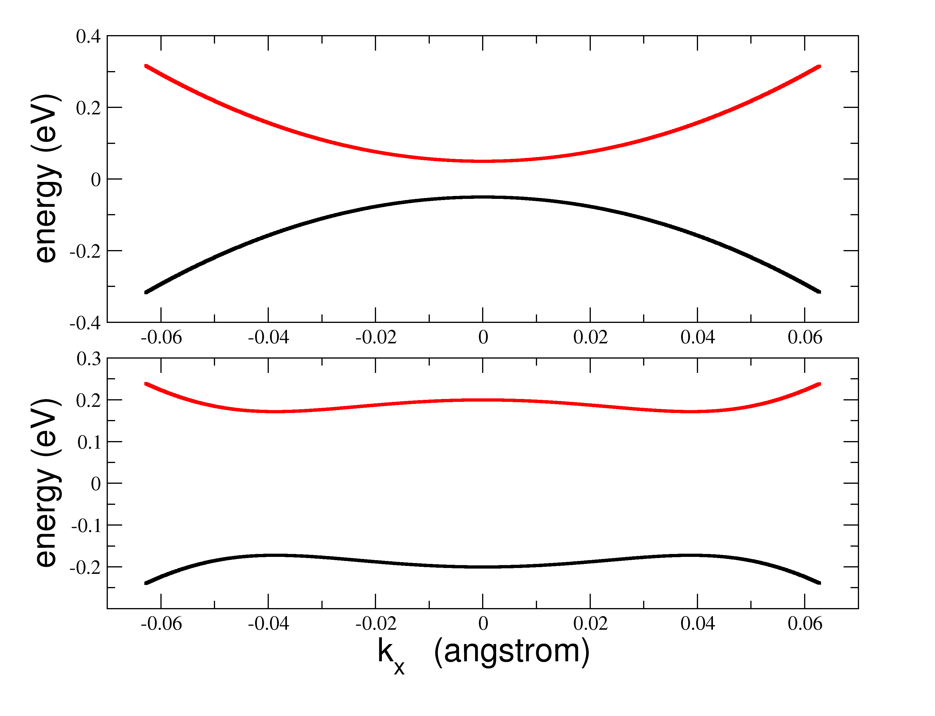
Figure 1: Band structure of the modified Dirac equation, as defined by Eq. (3), for $k_{y}=0$ as function of $k_{x}$. The used parameters are $v\hbar=3.65$ eV$\cdot$Å, $B\hbar^{2}$=-68 eV$\cdot$Ų, as for HgTe quantum wells. For $mv^{2}$ we take the value -0.05 eV for the upper panel and -0.2 for the lower panel. In the latter case the system is in the regime $2Bm>1$ and a Mexican-hat type of band is seen.

In Fig. 1, we depict the band structure of the modified Dirac equation in the regimes $2Bm\leq 1$ and $2Bm>1$ separately. It is clear that in the latter case the gap is off the $\Gamma-$point. The band structure has, in this case, a Mexican hat shape. Then, there is a full circumference in momentum space where the group velocity is zero and this has consequences in the density of state, as we shall see below. Although we are using for the parameters $v\hbar$ and $B\hbar^{2}$ those of HgTe quantum wells we make no claim that our results are directly applicable to that particular system, since the value we use for $mv^{2}$ is different from what is reported in the literature [10]. We simply fix $mv^{2}$ to a value that places the system in the regime $2Bm>1$.

The different behaviour of the system when $Bm$ is either positive or negative can also be seen from the average value of the spin operator, defined as

$$\bm{s}=(\sigma_{x},\sigma_{y},\sigma_{z})\,.$$ (8)

The several terms are

$$\langle\psi_{\bm{k},\pm}|\sigma_{x}|\psi_{\bm{k},\pm}\rangle = \pm\frac{k_{x}v\hbar}{E_{\bm{k}+}}\,,$$

$$\langle\psi_{\bm{k},\pm}|\sigma_{y}|\psi_{\bm{k},\pm}\rangle = \pm\frac{k_{y}v\hbar}{E_{\bm{k}+}}\,,$$

$$\langle\psi_{\bm{k},\pm}|\sigma_{z}|\psi_{\bm{k},\pm}\rangle = \pm\frac{mv^{2}-B\hbar^{2}k^{2}}{E_{\bm{k}+}}\,.$$ (9)

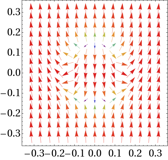
Figure 2: Vector plot of $\langle\psi_{\bm{k},+}|\sigma_{x}|\psi_{\bm{k},+}\rangle$ and $\langle\psi_{\bm{k},+}|\sigma_{z}|\psi_{\bm{k},+}\rangle$ as function of $k_{x}$ and $k_{y}$, expressed in Å. The used parameters are $v\hbar=3.65$ eV$\cdot$Å, $B\hbar^{2}$=-68 eV$\cdot$Ų, as for HgTe quantum wells. For $mv^{2}$ we take the value -1.5 eV, which puts the system in the regime $Bm>0$.

In Fig. 2 we depict a vector plot of $\langle\psi_{\bm{k},+}|\sigma_{x}|\psi_{\bm{k},+}\rangle$ and $\langle\psi_{\bm{k},+}|\sigma_{z}|\psi_{\bm{k},+}\rangle$ as function of $k_{x}$ and $k_{y}$, in the regime $Bm>0$. At the center of the Brillouin zone the spin points down whereas when we move off the center the spin rotates and at large momentum it points up; in the valence band the orientation of the spin is the opposite.

The situation is different when we consider the regime $Bm<0$, as shown in

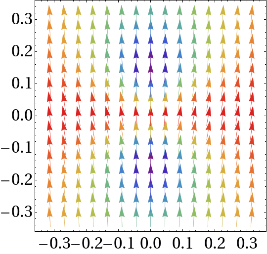
Figure 3: Vector plot of $\langle\psi_{\bm{k},+}|\sigma_{x}|\psi_{\bm{k},+}\rangle$ and $\langle\psi_{\bm{k},+}|\sigma_{z}|\psi_{\bm{k},+}\rangle$ as function of $k_{x}$ and $k_{y}$, expressed in Å. The used parameters are $v\hbar=3.65$ eV$\cdot$Å, $B\hbar^{2}$=-68 eV$\cdot$Ų, as for HgTe quantum wells. For $mv^{2}$ we take the value 1.5 eV, which puts the system in the regime $Bm<0$.

Fig. 3. In this case, the spin points along the same direction independent of the position in the Brillouin zone. The different behaviour of the spin, depending on the sign of the product $Bm$, is a manifestation of the trivial or non-trivial nature of the system.

The density of states (DOS) of the conduction band of the topological insulator defined by Hamiltonian 2 can be easily computed. This quantity is defined by the expression

$$\rho(\omega)=\frac{1}{A}\sum_{\bm{k}}\,\delta(\hbar\omega-E_{\bm{k},+})\,,$$ (10)

where $A$ is the area of the system and $E_{\bm{k},+}$ is given by 3 (with $\lambda=1$). Note that the expression for the DOS of the valence band can simply be obtained from the one above by replacing $\omega$ with $-\omega$, as $E_{\bm{k},-}=-E_{\bm{k},+}$. Converting the summation above in an integral over the Brillouin zone in the thermodynamic limit, and performing the angular integral, one obtains

$$\rho(\omega)=\frac{1}{4\pi}\,\int_{0}^{\infty}\,du\,\delta(\hbar\omega-E_{u,+})\,,$$ (11)

where we have performed the substitution $u=k^{2}$ in the integral over the modulus of the wave-vector, and where $E_{u,+}=\sqrt{v^{2}\hbar^{2}u+(mv^{2}-B\hbar^{2}u)^{2}}$.

The computation of the explicit expression for the DOS from 11 can be performed by determining the values of $u$ for which the argument of the delta function is zero in the expression above. Thus, we need to determine the roots of the equation $\hbar\omega=E_{u,+}$. Such roots will only contribute to the integral in 11 if they are real and positive.

We start by noting that from Eq. (3), we find that the minimum of the conduction band takes place at a momentum $k_{\Delta}$ given by

$$k_{\Delta}=v\frac{\sqrt{-1+2Bm}}{\sqrt{2}|B|\hbar}\,,$$ (12)

which implies that only for $2Bm>1$ does the minimum occurs off the $\Gamma-$point of the Brillouin zone. In this case, the band gap is

$$\Delta=\frac{v^{2}}{|B|}\sqrt{4Bm-1}\,,$$ (13)

and the dispersion resembles a Mexican hat, as is clearly seen in Fig. 1. If $2Bm<1$, the band gap occurs at the $\Gamma-$point and is given by $\Delta_{\Gamma}=2mv^{2}$. If the condition $2Bm>1$ is met, we always have $\Delta<\Delta_{\Gamma}$.

Taking into account the two different regimes $Bm<0$ and $Bm>0$ discussed above, and the appearance of a minimum of off the $\Gamma-$point for $2Bm>1$, we need to consider three different cases when analysing the roots of the equation $\hbar\omega=E_{u,+}$: (i) the trivial case, where $Bm<0$; (ii) the non-trivial case, where $Bm>0$ and $2Bm<1$; (iii) the non-trivial case, where $2Bm>1$. Defining $f(u)=\omega\hbar-E_{u,+}$, the zeros of $f(u)$, that is $f(u_{0})=0$, are

$$u_{0}=\left\{\begin{array}[]{c}u_{-}=-\frac{v^{2}(1-2Bm)}{2B^{2}\hbar^{2}}-\frac{g(B,m,\omega)}{2B^{2}\hbar^{2}}\\ u_{+}=-\frac{v^{2}(1-2Bm)}{2B^{2}\hbar^{2}}+\frac{g(B,m,\omega)}{2B^{2}\hbar^{2}}\\ \end{array}\right.\,,$$ (14)

where $g(B,m,\omega)$ is defined by

$$g(B,m,\omega)=\sqrt{v^{4}(1-4Bm)+4B^{2}\omega^{2}\hbar^{2}}\,.$$ (15)

Since the discriminant of the square root [in $g(B,m,\omega)$] has to be positive, we find that $\hbar\omega$ can have any positive value in both the trivial case and the non-trivial case if $4Bm<1$. For the non-trivial case when $4Bm>1$ we find that

$$\hbar\omega\geq\frac{v^{2}}{2|B|}\sqrt{4Bm-1}=\frac{\Delta}{2}\,.$$ (16)

If $u_{-}$ and $u_{+}$ are to contribute to the integration of the $\delta-$function, both have to be positive numbers. This imposes some restrictions on the values of $\hbar\omega$ depending on the $2Bm$ parameter. A detailed analysis reveals the following conclusions. In the trivial case, only $u_{+}$ is positive and therefore $u_{-}$ does not contributes to the integral. In this case, we find that $\hbar\omega$ has to satisfy the condition $\hbar\omega>mv^{2}=\frac{\Delta_{\Gamma}}{2}$. In the non trivial case, we have two regimes to consider: when (i) $2Bm<$1 and when (ii) $2Bm>1$. In case (i), only the root $u_{+}$ contributes and the frequency $\omega$ has to satisfy the condition $\hbar\omega>\frac{\Delta_{\Gamma}}{2}$. In case (ii), both roots contribute. The root $u_{-}$ gives a contribution in the energy range $\frac{\Delta}{2}<\hbar\omega<\frac{\Delta_{\Gamma}}{2}$, whereas the root $u_{+}$ gives a contribution in the region $\hbar\omega>\frac{\Delta}{2}$. Taking such information into account when computing the integral in 11, we obtain, using the properties of the delta function, the result

$$\rho(\omega)=\left\{\begin{array}[]{c}\frac{\omega\,\theta(\omega-\Delta_{\Gamma}/2)}{4\pi\hbar\sqrt{v^{4}(1-4mB)+4B^{2}\omega^{2}\hbar^{2}}}\;\;\mbox{if}\;\;2mB<1\\ \frac{\omega\,(1+\tilde{\theta}(\Delta_{\Gamma}/2-\omega))\,\theta(\omega-\Delta/2)}{4\pi\hbar\sqrt{v^{4}(1-4mB)+4B^{2}\omega^{2}\hbar^{2}}}\,\;\;\mbox{if}\;\;2mB\geq 1\\ \end{array}\right.\,,$$ (17)

where $\theta(x)=0$, if $x<0$, $\theta(x)=1/2$, if $x=0$, and $\theta(x)=1$, if $x>0$, and where $\tilde{\theta}(x)=0$, if $x<0$, and $\tilde{\theta}(x)=1$, if $x\geq 0$. A plot of this quantity for selected values of the different parameters is given in Fig. 4. Note the appearance of a peak and a discontinuity in the DOS, in the frequency range $\frac{\Delta}{2}<\hbar\omega<\frac{\Delta_{\Gamma}}{2}$, for $2mB\geq 1$, signalling the change of regime pointed above.

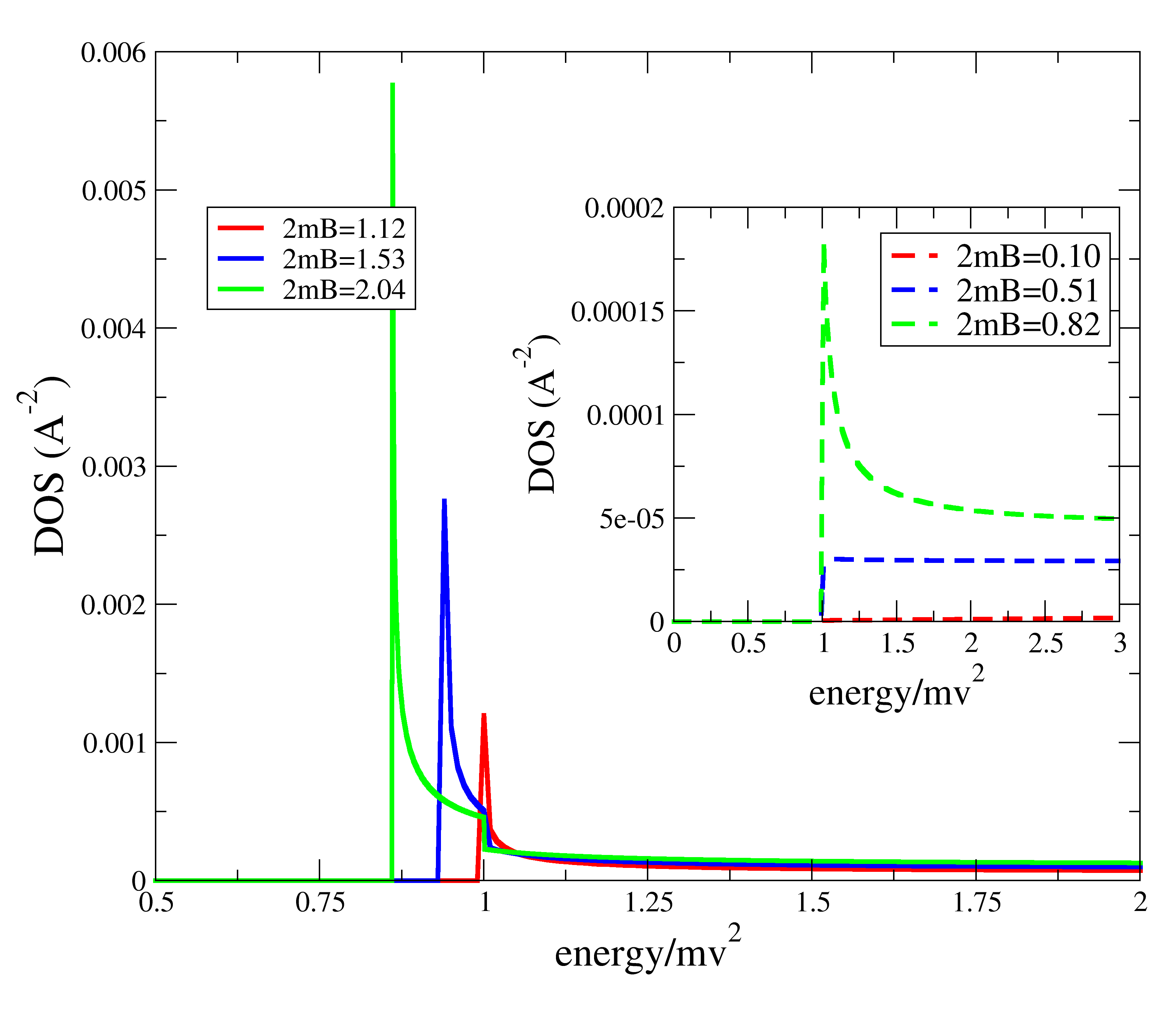
Figure 4: DOS of a modified Dirac equation, as given by equation 17. The function was scaled by a factor of $mv^{2}$ so that the area under the curve is preserved with respect to the result given in 17, given that the energy is expressed here in units of $mv^{2}$ as well. The used parameters are $v\hbar=3.65$ eV$\cdot$Å, $B\hbar^{2}$=-68 eV$\cdot$Ų, as for HgTe quantum wells.

3 Kubo formula: fixing notation

From linear response, we know that the average of the current operator is given by

$$\langle J_{\alpha}\rangle=-\frac{i}{\hbar}\int_{-\infty}^{t}dt^{\prime}\langle[J_{\alpha}(t),V(t^{\prime})]\rangle\,,$$ (18)

where $V(t)$ is the perturbation. We consider an Hamiltonian, $H(\hbar\bm{k})$, such that the electrons couple to the electromagnetic field through minimal coupling, that is,

$$H=H(\hbar\bm{k}-q\bm{A})\,,$$ (19)

where $q$ is the charge of the particles (for electrons we have $q=-e$, with $e>0$). The current is defined as

$$J_{\gamma}=-\frac{\partial H}{\partial A_{\gamma}}=\frac{q}{\hbar}\frac{\partial H(\hbar\bm{k})}{\partial k_{\gamma}}\,,$$ (20)

and for a small $q\bm{A}$ (linear response) we have

$$H(\hbar\bm{k}-q\bm{A}) \approx H(\hbar\bm{k})-\sum_{\gamma}qA_{\gamma}\frac{\partial H(\hbar\bm{k})}{\hbar\partial k_{\gamma}}$$ (21)

$$= H(\hbar\bm{k})-\sum_{\gamma}J_{\gamma}A_{\gamma},$$

thus, the perturbation reads

$$V(t)=-\sum_{\gamma}J_{\gamma}A_{\gamma}(t)\,,$$ (22)

where we have assumed that $A_{\gamma}(t)$ is a function of time. Then, the average of the $\alpha-$component of the current is

$$\langle J_{\alpha}\rangle=\sum_{\gamma}\frac{i}{\hbar}\int_{-\infty}^{t}dt^{\prime}\langle[J_{\alpha}(t),J_{\gamma}(t^{\prime})]\rangle A_{\gamma}(t^{\prime})\,,$$ (23)

where $J_{\alpha}(t)$ is the current operator in the interaction picture. We can now introduce a retarded function defined as

$$\Pi^{R}_{\alpha\gamma}(t-t^{\prime})=-i\theta(t-t^{\prime})\langle[J_{\alpha}(t),J_{\gamma}(t^{\prime})]\rangle\,,$$ (24)

such that

$$\langle J_{\alpha}\rangle=\sum_{\gamma}\frac{-1}{\hbar}\int_{-\infty}^{\infty}\Pi^{R}_{\alpha\gamma}(t-t^{\prime})A_{\gamma}(t^{\prime})\,.$$ (25)

Fourier transforming the previous equation we obtain

$$\langle J_{\alpha}(\omega)\rangle=-\frac{1}{\hbar}\sum_{\gamma}\Pi^{R}_{\alpha\gamma}(\omega)A_{\gamma}(\omega)\,.$$ (26)

If we now choose

$$A_{\gamma}(t) = A_{\gamma}(\omega)e^{-i\omega t}$$ (27)

$$\Rightarrow E_{\gamma}=-\frac{\partial A_{\gamma}(t)}{\partial t}=i\omega A_{\gamma}(\omega)e^{.i\omega t}\,,$$

thus $A_{\gamma}(\omega)=-iE(\omega)/\omega$. Finally, the conductivity tensor is

$$\sigma_{\alpha\gamma}(\omega)=\frac{i}{\hbar\omega}\Pi^{R}_{\alpha\gamma}(\omega)\,.$$ (28)

The retarded current-current correlation function is computed from the Matsubara correlation function, which is defined as

$$\Pi_{\alpha\gamma}(i\omega_{n})=\int_{0}^{\beta\hbar}d\tau e^{i\omega_{n}\tau}\Pi_{\alpha\gamma}(\tau)\,,$$ (29)

where

$$\Pi_{\alpha\gamma}(\tau)=-\langle T_{\tau}J_{\alpha}(\tau)J_{\gamma}(0)\rangle\,,$$ (30)

and $\beta=1/(k_{B}T)$, where $k_{B}$ is the Boltzmann constant and $T$ the temperature.

4 Optical conductivity of a two-band Hamiltonian: formal matters

In connection with the Hamiltonian (2), let us now define creation and annihilation operators, $a^{\dagger}_{\bm{k},\lambda}$ and $a_{\bm{k},\lambda}$, which create and annihilate electrons in the band $\lambda$ with momentum $\hbar\bm{k}$; we denote $\lambda=+$ for the conduction band and $\lambda=-$ for the valence band. In this basis, the current operators in second quantization are defined as

$$\hat{J}_{x}=\sum_{\bm{k},\lambda,\lambda^{\prime}}a^{\dagger}_{\bm{k},\lambda}a_{\bm{k},\lambda^{\prime}}\langle\psi_{\bm{k},\lambda}|J_{x}|\psi_{\bm{k},\lambda^{\prime}}\rangle\,,$$ (31)

$$\hat{J}_{y}=\sum_{\bm{k},\lambda,\lambda^{\prime}}a^{\dagger}_{\bm{k},\lambda}a_{\bm{k},\lambda^{\prime}}\langle\psi_{\bm{k},\lambda}|J_{y}|\psi_{\bm{k},\lambda^{\prime}}\rangle\,,$$ (32)

where $J_{\alpha}$, ($\alpha=x,y$) is defined in Eq. (20).

In second quantization the Matsubara current-current correlation function is written as

$$\Pi_{\alpha\gamma}(i\omega_{n})=-\int_{0}^{\beta\hbar}d\tau e^{i\omega_{n}\tau}\sum_{\bm{k}_{1},\lambda_{1},\lambda^{\prime}_{1}}\sum_{\bm{k}_{2},\lambda_{2},\lambda^{\prime}_{2}}$$

$$\langle\psi_{\bm{k}_{1},\lambda_{1}}|J_{\alpha}|\psi_{\bm{k}_{1},\lambda^{\prime}_{1}}\rangle\langle\psi_{\bm{k}_{2},\lambda_{2}}|J_{\gamma}|\psi_{\bm{k}_{2},\lambda^{\prime}_{2}}\rangle$$

$$\times\langle a^{\dagger}_{\bm{k}_{1},\lambda_{1}}a_{\bm{k}_{1},\lambda_{1}}a^{\dagger}_{\bm{k}_{2},\lambda_{2}}a_{\bm{k}_{2},\lambda^{\prime}_{2}}\rangle\,,$$ (33)

which in terms of Green’s functions reads

$$\Pi_{\alpha\gamma}(i\omega_{n})=-\int_{0}^{\beta\hbar}d\tau e^{i\omega_{n}\tau}\sum_{\bm{k}_{1},\lambda_{1},\lambda^{\prime}_{1}}\sum_{\bm{k}_{2},\lambda_{2},\lambda^{\prime}_{2}}$$

$$\langle\psi_{\bm{k}_{1},\lambda_{1}}|J_{\alpha}|\psi_{\bm{k}_{1},\lambda^{\prime}_{1}}\rangle\langle\psi_{\bm{k}_{2},\lambda_{2}}|J_{\gamma}|\psi_{\bm{k}_{2},\lambda^{\prime}_{2}}\rangle$$

$$\times{\cal G}(\bm{k}_{1},\lambda_{1},\tau)\delta_{\bm{k}_{1},\bm{k}_{2}}\delta_{\lambda^{\prime}_{2},\lambda_{1}}{\cal G}(\bm{k}_{1},\lambda^{\prime}_{1},-\tau)\delta_{\bm{k}_{1},\bm{k}_{2}}\delta_{\lambda_{2},\lambda^{\prime}_{1}}\,,$$ (34)

where

$${\cal G}(\bm{k},\lambda,\tau)=-\langle T_{\tau}a_{\bm{k},\lambda}a^{\dagger}_{\bm{k},\lambda}(\tau)\rangle\,.$$ (35)

Introducing the Fourier representation

$${\cal G}(\bm{k},\lambda,\tau)=\frac{1}{\hbar\beta}\sum_{i\omega_{1}}e^{-i\omega_{1}\tau}{\cal G}(\bm{k},\lambda,i\omega_{1})\,,$$ (36)

we obtain

$$\Pi_{\alpha\gamma}(i\omega_{n})=\sum_{\bm{k},\lambda,\lambda^{\prime}}\langle\psi_{\bm{k},\lambda}|J_{\alpha}|\psi_{\bm{k},\lambda^{\prime}}\rangle\langle\psi_{\bm{k},\lambda^{\prime}}|J_{\gamma}|\psi_{\bm{k},\lambda}\rangle$$

$$\times\frac{1}{\beta\hbar}\sum_{i\omega_{2}}{\cal G}(\bm{k},\lambda,i\omega_{n}+i\omega_{2}){\cal G}(\bm{k},\lambda^{\prime},i\omega_{2})$$ (37)

which after summing over the Matsubara frequency $\omega_{2}$ gives

$$\Pi_{\alpha\gamma}(i\omega_{n})=\sum_{\bm{k},\lambda,\lambda^{\prime}}\langle\psi_{\bm{k},\lambda}|J_{\alpha}|\psi_{\bm{k},\lambda^{\prime}}\rangle\langle\psi_{\bm{k},\lambda^{\prime}}|J_{\gamma}|\psi_{\bm{k},\lambda}\rangle$$

$$\times\frac{n_{F}(\bm{k},\lambda^{\prime})-n_{F}(\bm{k},\lambda)}{i\omega_{n}+(E_{\bm{k},\lambda^{\prime}}-E_{\bm{k},\lambda^{\prime}})/\hbar}\,,$$ (38)

where $n_{F}(x)$ is the Fermi distribution function. For $\lambda=\lambda^{\prime}$ the previous result is zero due to the Fermi functions. Finally, the retarded current-current correlation function is obtained from the Matsubara one by analytical continuation $\Pi^{R}_{\alpha\gamma}(\omega)=\Pi_{\alpha\gamma}(i\omega_{n}\rightarrow\omega+i0^{+})$. Since

$$\sigma_{\alpha\gamma}(\omega)=\frac{i}{\hbar\omega}\Pi^{R}_{\alpha\gamma}(\omega)\,,$$ (39)

the real part of the conductivity tensor is given by

$$\Re\sigma_{\alpha\gamma}(\omega)=\frac{i}{\hbar\omega}i\Im\Pi^{R}_{\alpha\gamma}(\omega)=-\frac{\Im\Pi^{R}_{\alpha\gamma}(\omega)}{\hbar\omega}\,.$$ (40)

From here on, we will be interested in the diagonal component of the conductivity tensor.

5 Optical conductivity of a modified Dirac equation

As already noted, the retarded current-current correlation function $\Pi^{R}_{xx}(\omega)$ can be obtained by analytical continuation of the Matsubara current-current correlation function, leading to an imaginary part of the form

$$\Im\Pi^{R}_{xx}(\omega)=\frac{-\pi}{A}\sum_{\bm{k},\lambda\neq\lambda^{\prime}}|\langle\psi_{\bm{k},\lambda}|J_{x}|\psi_{\bm{k},\lambda^{\prime}}\rangle|^{2}$$

$$\times[n_{F}(\bm{k},\lambda^{\prime})-n_{F}(\bm{k},\lambda)]\delta[\omega+(E_{\bm{k},\lambda^{\prime}}-E_{\bm{k},\lambda^{\prime}})/\hbar]\,,$$ (41)

where $A$ is the area of the system. The current operator $J_{x}$ is defined as

$$J_{x}=-\frac{e}{\hbar}\sum_{\alpha}\partial_{k_{x}}d_{\alpha}(\bm{k})\sigma_{\alpha}\,,$$ (42)

which we use in the calculation of the matrix elements entering in Eq. (41). In the thermodynamic limit, the momentum summation in Eq. (41) transforms into an integral in the usual way and one has to compute the angular average of the matrix elements, that is,

$$I(k)=\int_{0}^{2\pi}d\theta|\langle\psi_{\bm{k},\lambda}|J_{x}|\psi_{\bm{k},\lambda^{\prime}}\rangle|^{2}\,.$$ (43)

The final result is $I(k)={\cal K}(k)\,,$ where

$${\cal K}(k) = \frac{\pi\hbar^{2}}{E^{2}_{\bm{k},+}}[v^{2}(E^{2}_{\bm{k},+}+M^{2}(\bm{k}))$$ (44)

$$+ 4BkM(\bm{k})v\hbar\sqrt{E^{2}_{\bm{k},+}-M^{2}(\bm{k})}$$

$$+ 4B^{2}\hbar^{2}k^{2}(E^{2}_{\bm{k},+}-M^{2}(\bm{k}))]\,.$$

The imaginary part part of the current-current correlation function reads

$$\Im\Pi^{R}_{xx}(\omega) = -\frac{e^{2}}{\hbar}\pi\int_{0}^{\infty}\frac{du}{8\pi^{2}}{\cal K}(u)\delta(\omega\hbar-2E_{u,+})\times$$ (45)

$$[n_{F}(-\hbar\omega/2)-n_{F}(\hbar\omega/2)]\,,$$

where the change of variable $u=k^{2}$ was again made. In what follows, we assume that the chemical potential lies in the energy gap and we take the zero temperature limit; for finite temperatures, we have to keep the Fermi functions. If we take the limit $m,B\rightarrow 0$, the real part of the conductivity reads

$$\Re\sigma_{xx}(\omega)=\frac{\sigma_{0}}{4}\,,$$ (46)

which is 1/4 the universal conductivity of neutral graphene, since we have not considered spin, and in this case there is not a two-valley degeneracy as there is in graphene. In the case $B=0$, the conductivity reads

$$\Re\sigma_{xx}(\omega)=\frac{\sigma_{0}}{4}\left(1+\frac{m^{2}v^{4}}{\hbar^{2}\omega^{2}}\right)\,,$$ (47)

for values of $\hbar\omega$ greater than $2mv^{2}$. In this case, the optical conductivity is at most $5\sigma_{0}/16$.

In the general case, of finite $B$ and $m$, we need again to evaluate the integration of the $\delta-$function to obtain $\Re\sigma_{xx}(\omega)$. The discussion is analogous to the one made for the DOS, one merely needs to replace $\hbar\omega$ with $\hbar\omega/2$. The analytical expression for the optical conductivity when both $B$ and $m$ are finite is too cumbersome to be given here and not much insight is gained.

In Fig. 5, we plot the optical conductivity of the modified Dirac equation. In the left panel, we follow the evolution of the optical conductivity upon the parameter $2Bm$. It is clear that as this parameter increases so does the optical conductivity, specially close to the gap edge. When $2Bm$ approach 1 the conductivity is greatly enhanced close to the edge of the gap $\Delta_{\Gamma}$. When the system enters the regime $2Bm>1$ the conductivity can be enhanced by more than one order of magnitude for photon energies satisfying the relation $\hbar\omega\gtrsim\Delta$. Thus we find a strong light-matter interaction in the non-trivial regime for $2Bm>1$. A particular feature of this regime is a jump in the conductivity at $\hbar\omega=\Delta_{\Gamma}$. This jump correlates with the same behaviour seen in the density of states and is a signature that the system is in the non-trivial regime.

Finally, we have found that in the trivial regime the optical conductivity of the bulk system is of the order of magnitude as that measured for graphene.

Figure 5: Optical conductivity of the modified Dirac equation. The used parameters are $v\hbar=3.65$ eV$\cdot$Å, $B\hbar^{2}$=-68 eV$\cdot$Ų, as for HgTe quantum wells. The dashed line in the left panel is the result given by Eq. (46). The conductivity is in units of $\sigma_{0}$ and the photon energy in units of $\Delta_{\Gamma}=2mv^{2}$.

6 Conclusions

We have discussed several aspects of the modified Dirac equation. We computed the Chern number which defines the trivial and non-trivial regimes of the system. We then computed the density of states and the optical conductivity of the modified Dirac equation. We found that in the non-trivial regime, characterized by $2Bm>1$, the density of states diverges as the energy approaches $\hbar\omega=\Delta$ and that the optical conductivity is greatly enhanced relatively to the case where $0<2Bm\ll 1$. Indeed, the divergence in the density of states also appears in the optical conductivity at photon energies close to $\Delta$. This divergence configures a strong light-matter interaction for that range of frequencies. We then expect that physical effects such as the Faraday rotation [19, 20] must exhibit dramatic results, when compared to the case of graphene, in the quantum regime dominated by inter-band transitions. Finally, we are confident that in the realm of cold atoms the parameters $B$, $m$ and $v$ can be tuned at will, making possible the external tuning of the several regimes and the observation of the different effects proposed here.

References

References

[1]
Fox M 2010 Optical Properties of Solids 2nd ed (Oxford)
[2]
Castro Neto A H, Guinea F, Peres N M R, Novoselov K S and Geim A K 2009 Rev. Mod. Phys.81 109
[3]
Peres N M R 2010 Rev. Mod. Phys.82 2673
[4]
Qi X L and Zhang S C 2010 Physics Today63 33
[5]
Manoharan H C 2010 Nature Nanotechnology477 33
[6]
Kane C and Moore J 2011 Physics World24 32
[7]
Bernevig B A 2013 Topological Insulators and Topological
Superconductors (Princeton)
[8]
Zhang H, Liu C X, Qi X L, Dai X, Fang Z and Zhang S C 2009 Nature
Physics5 438
[9]
Hasan M Z and Kane C L 2010 Rev. Mod. Phys.82 3045
[10]
Qi X L and Zhang S C 2011 Rev. Mod. Phys.83 1057
[11]
Li Z and Carbotte J P 2013 Phys. Rev. B87 155416
[12]
Nair R R, Blake P, Grigorenko A N, Novoselov K S, Booth T J, Stauber T, Peres
N M R and Geim A 2008 Science320 1308
[13]
Stauber T, Peres N M R and Geim A K 2008 Phys. Rev. B78 085432
[14]
Schmeltzer D and Ziegler K 2013 arXiv:1302.4145
[15]
LaForge A D, Frenzel A, Pursley B C, Lin T, Liu X, Shi J and Basov D N 2010
Phys. Rev. B81 125120
[16]
Pietro P D, Vitucci F M, Nicoletti D, Baldassarre L, Calvani P, Cava R, Hor
Y S, Schade U and Lupi S 2012 Phys. Rev. B86 045439
[17]
Akrap A, Tran M, Ubaldini A, Teyssier J, Giannini E, van der Marel D, Lerch P
and Homes C C 2012 Phys. Rev. B86 235207
[18]
Shen S Q, Shan W Y and Lu H Z 2011 SPIN1 1
[19]
Ubrig N, Crassee I, Levallois J, Nedoliuk I O, Fromm F, Kaiser M, Seyller T and
Kuzmenko A B 2011 Nature Physics7 48
[20]
Ferreira A, Viana-Gomes J, Bludov Y V, Pereira V, Peres N M R and Castro Neto
A H 2011 Phys. Rev. B84 235410