Suppression of Coulomb exchange energy in quasi-two-dimensional hole systems

Abstract

We have calculated the exchange-energy contribution to the total energy of quasi-two-dimensional hole systems realized by a hard-wall quantum-well confinement of valence-band states in typical semiconductors. The magnitude of the exchange energy turns out to be suppressed from the value expected for analogous conduction-band systems whenever the mixing between heavy-hole and light-hole components is strong. Our results are obtained using a very general formalism for calculating the exchange energy of many-particle systems where single-particle states are spinors. We have applied this formalism to obtain analytical results for spin-3/2 hole systems in limiting cases.

I Introduction and overview of main results

In many cases, Coulomb interactions in many-electron systems can be accounted for by perturbation theory Giuliani and Vignale (2005). This is usually possible at sufficiently high densities where the single-particle (kinetic-energy or band-dispersion) contribution to the ground-state energy dominates. In lowest order, interactions give rise to the Hartree and exchange-interaction terms. The Hartree term embodies the purely electrostatic Coulomb potential energy of the electrons. In a uniform system, the Hartree contribution is cancelled by the neutralizing background of ionic charges in the solid. What remains is the exchange term, which we focus on in this work.

Since their experimental realization, quantum-confined systems have become attractive laboratories for the study of interacting electrons because interaction effects are enhanced in low spatial dimensions Giuliani and Vignale (2005). Examples include the exchange enhancement of parameters such as spin susceptibility and effective mass in quasi-two-dimensional (quasi-2D) conduction-band electron systems Smith and Stiles (1972); Tanatar and Ceperley (1989); Attaccalite et al. (2002). Curiously, experiments on similarly confined valence-band (hole) states seem to indicate the absence of exchange-related renormalizations of electronic parameters Pinczuk et al. (1986); Winkler et al. (2005); Chiu et al. (2011). Here we reveal a possible origin of this suppression of interaction effects in quasi-2D hole systems: the high effective spin associated with valence-band states. Peculiar Coulombic effects arising from the spin-3/2 character of holes have previously been noted for bulk semiconductors. Combescot and Nozières (1972); Schliemann (2006, 2011); Kyrychenko and Ullrich (2011) More recent theoretical studies have focused also on quasi-2D hole gases. Schmitt (1994); Cheng and Gerhardts (2001); Kernreiter et al. (2010, 2013); Scholz et al. (2013) Our results provide new insight into the effect of valence-band mixing on physical properties of confined holes, and the formalism developed here can also form the basis for further detailed studies of interaction phenomena in experimentally realized quasi-2D hole systems.

The multi-band envelope function approach to electron states in crystalline solids implies that eigenstates are (in principle, infinite-dimensional) spinors Yu and Cardona (2010) which affect the matrix elements describing physical processes in important ways. For an $n$-fold degenerate band, we may often restrict ourselves to $n$ spinors. The states in the lowest conduction band are usually non-degenerate, except for spin, so that the spinor structure may often be ignored. A nontrivial example are hole states in the topmost valence band of common semiconductors such as Si, Ge, GaAs, InAs, and CdTe. The bulk valence band in these materials is four-fold degenerate at the band edge, corresponding to an effective spin 3/2. Away from the band edge, the dispersion splits into the doubly degenerate heavy-hole (HH) and light-hole (LH) bands. In quasi-2D systems, the quantum-well confinement results in an energy splitting between HH and LH bands such that the subbands are only two-fold degenerate, even at the subband edge with in-plane wave vector $|{\bm{\mathrm{k}}}|\equiv k=0$. Nevertheless, states in these subbands need to be described by four-spinors and, except at $k=0$, these are never pure HHs or LHs. Figure 1 shows the subbands obtained for a hard-wall confinement of holes within the axial approximation for three semiconductor materials. The nontrivial physics arises due to the fact that the degeneracy of the subbands at any fixed value of energy and wave vector ${\bm{\mathrm{k}}}$ is lower than the number of spinors needed to describe the dynamics of the Bloch waves. Similar physics applies also to, e.g., 2D electron systems with Rashba spin-orbit (SO) coupling. Rashba (1960); Bychkov and Rashba (1984); Winkler (2003) However, it was found that the exchange energy of such systems deviates only marginally from that of a simple 2D electron gas Chesi and Giuliani (2007, 2011), while the properties of collective excitations can be more strongly affected by SO coupling Agarwal et al. (2011).

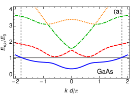
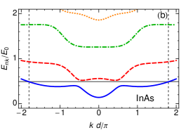
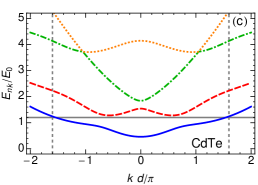
Figure 1: Lowest (doubly degenerate) subbands of 2D hole systems realized by a hard-wall confinement of width $d$, for (a) GaAs, (b) InAs, and (c) CdTe. $E_{0}=\pi^{2}\hbar^{2}/(2m_{0}d^{2})$ is the appropriate size-quantization energy scale. Gray lines delimit the range of energies and wave vectors for which only the lowest subband is occupied, which is the regime we focus on in this work.

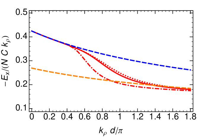
Figure 2: Exchange energy per particle $E_{\mathrm{X}}/N$ for a hard-wall-confined quasi-2D hole system in GaAs (solid red curve), InAs (dash-dotted red curve), and CdTe (dotted red curve). $C\equiv e^{2}/(4\pi\epsilon\epsilon_{0})$ is the Coulomb-interaction constant, $k_{\rho}$ denotes the Fermi wave vector, and $d$ is the quantum-well width. The blue dashed curve shows the result (2) based on the EMA. The orange dashed curve is $E_{\mathrm{X}}/N$ for a spin-3/2 hole system described by a multi-spinor wave function with equal amplitudes for the heavy-hole and light-hole components.

As a reference for our discussion below, we briefly review the textbook problem Giuliani and Vignale (2005) of the exchange energy per particle for a 2D electron gas with zero thickness perpendicular to the 2D plane, giving Chaplik (1971); Stern (1973); Giuliani and Vignale (2005)

$$\frac{E_{\mathrm{X}}^{(0)}}{N}=-\frac{4C}{3\pi}\,k_{\rho}\equiv-\frac{4}{3}\,\sqrt{\frac{2}{\pi}}\;C\,\sqrt{\rho}=:\varepsilon_{\mathrm{X}}\quad.$$ (1)

Here $N$ is the number of electrons, $C\equiv e^{2}/(4\pi\epsilon\epsilon_{0})$ is the Coulomb-interaction constant, $\rho$ is the electron sheet density, and $k_{\rho}=\sqrt{2\pi\rho}$ denotes the Fermi wave vector. This result is based on the following assumptions. (i) The in-plane orbital motion is fully characterized by plane waves. (ii) We have a two-fold spin degeneracy of the energy eigenstates, implying that all energy eigenstates can simultaneously be chosen as eigenstates of spin projection on a fixed axis. The latter manifests itself in the fact that only interactions between particles with the same spin projections contribute to the exchange energy. We emphasize these well-known points because we find below that these assumptions are not applicable for quasi-2D hole systems.

Using the same assumptions (i) and (ii) above, one can evaluate the exchange energy for a quasi-2D electron gas in the lowest subband of a quantum well with hard-wall confinement. Here, $E_{\mathrm{X}}$ depends also on the well width $d$ and can be written as Betbeder-Matibet et al. (1994, 1996)

$$\frac{E_{\mathrm{X}}^{(\mathrm{EMA})}}{N}=\varepsilon_{\mathrm{X}}\,\Lambda^{\mathrm{(\mathrm{EMA})}}(k_{\rho}d)\quad.$$ (2)

The universal function $\Lambda^{\mathrm{(\mathrm{EMA})}}(k_{\rho}d)$ was expressed in Ref. Betbeder-Matibet et al., 1996 in terms of a Taylor expansion in its argument. In the following, we will refer to Eq. (2) as the effective-mass approximation (EMA) to the exchange energy. We note that the exchange energy in quasi-2D systems is generally reduced with increasing quantum-well width $d$.

Frequently the exchange energy is expressed in terms of the dimensionless density parameter $r_{s}$, which in 2D is the ratio between the Coulomb energy $C\sqrt{\pi\rho}$ and the kinetic energy $\pi\rho\,\hbar^{2}/m^{\ast}$, assuming a parabolic dispersion $E_{\bm{\mathrm{k}}}=\hbar^{2}k^{2}/(2m^{\ast})$ with effective mass $m^{\ast}$. In the current work, we avoid using the parameter $r_{s}=m^{\ast}C/(\hbar^{2}\sqrt{\pi\rho})$, the reason being that the systems we study here do not have a simple parabolic energy dispersion.

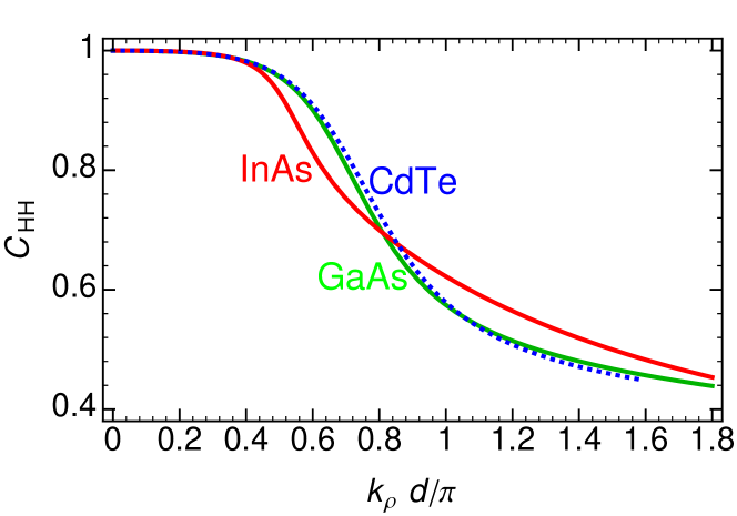
Figure 3: Heavy-hole (HH) character of states at the Fermi energy in the lowest subband, as measured by $C_{\mathrm{HH}}$, which is the combined integrated probability density of the HH entries in the confined-hole spinor wave function. (See text for details.)

Using the numerically calculated multi-spinor envelope functions for quasi-2D hole systems, we evaluate their exchange energy and find it to deviate from the EMA expression (2). As Fig. 2 shows, the EMA behavior is exhibited in the low-density, small-width limit where the system’s states are essentially HH-like Winkler (2003). However, at larger densities, even with still only the lowest quasi-2D subband occupied, the character of the wave functions becomes mixed, with eventually the HH and LH components having almost equal weight (see Fig. 3 and Ref. Winkler, 2003). The exchange energy turns out to be suppressed compared to the EMA value as soon as the contributions from LH components become significant. This can be seen from Fig. 3 in conjunction with Fig. 2. We obtain good agreement between the asymptotic behavior of $E_{\mathrm{X}}$ at large densities and an analytical expression obtained within a simplified model with equally distributed HH and LH amplitudes. This supports our hypothesis that the suppression of exchange effects in quasi-2D hole systems arises as a consequence of valence-band mixing.

In the remainder of this paper, we provide details of the calculations and further information to illustrate our conclusions. The basic formalism for calculating the exchange energy of quasi-2D systems is described in Sec. II. In Sec. III, we review known results for quasi-2D spin-1/2 electron systems that provide a benchmark for comparison with analogous hole systems. The formalism for calculating the exchange energy of spin-3/2 quasi-2D hole systems and a discussion of the obtained results are given in Sec. IV. The conclusions of our work are summarized in the final Sec. V.

II Exchange energy of quasi-2D systems

II.1 General formalism

In its most general form, the many-body Hamiltonian of interacting band electrons reads

$$\mathcal{H} = \sum_{n,{\bm{\mathrm{k}}}}E_{n{\bm{\mathrm{k}}}}~{}\hat{c}_{n{\bm{\mathrm{k}}}}^{\dagger}\hat{c}_{n{\bm{\mathrm{k}}}}+\frac{1}{2A}\sum_{n_{i},{\bm{\mathrm{k}}},{\bm{\mathrm{k}}}^{\prime},{\bm{\mathrm{q}}}\neq 0}V^{n_{1}n_{2}}_{n_{3}n_{4}}({\bm{\mathrm{k}}},{\bm{\mathrm{k}}}^{\prime},{\bm{\mathrm{q}}})$$ (3)

$$\hskip 56.9055pt{}\times\hat{c}_{n_{1}{\bm{\mathrm{k}}}+{\bm{\mathrm{q}}}}^{\dagger}\hat{c}_{n_{2}{\bm{\mathrm{k}}}^{\prime}-{\bm{\mathrm{q}}}}^{\dagger}\hat{c}_{n_{3}{\bm{\mathrm{k}}}^{\prime}}\hat{c}_{n_{4}{\bm{\mathrm{k}}}}\quad,$$

where $A$ is the system volume (i.e., area in the 2D case), and the operators $\hat{c}_{n{\bm{\mathrm{k}}}}$ ($\hat{c}_{n{\bm{\mathrm{k}}}}^{\dagger}$) annihilate (create) an electron with wave vector ${\bm{\mathrm{k}}}$. Note that in the presence of SO interaction the spin quantum number is, by itself, not a good quantum number. Thus $n$ is a common index for the orbital motion in a (sub)band and the spin degree of freedom. Winkler (2003) In the following, we focus on the case of a quantum-well-confined system, hence the indices $n_{i}$ are labeling quasi-2D subbands and ${\bm{\mathrm{k}}}\equiv(k_{x},k_{y})$ is a 2D vector. We use the jellium model and therefore the $\mathbf{q}=\mathbf{0}$ component of the interaction is not present, as it cancels with the external potential due to the homogeneous positive-charge background that ensures charge neutrality. Treating the interaction part of the Hamiltonian in first-order perturbation theory gives the following correction to the expectation value of the energy of the system:

$$\begin{array}[b]{@{}>{\displaystyle}r@{}}E_{\mathrm{X}}=-\frac{1}{2A}\sum_{n_{i},{\bm{\mathrm{k}}},{\bm{\mathrm{k}}}^{\prime},{\bm{\mathrm{q}}}\neq 0}V^{n_{1}n_{2}}_{n_{3}n_{4}}({\bm{\mathrm{k}}},{\bm{\mathrm{k}}}^{\prime},{\bm{\mathrm{q}}})\;\langle\hat{c}_{n_{1}{\bm{\mathrm{k}}}+{\bm{\mathrm{q}}}}^{\dagger}\hat{c}_{n_{3}{\bm{\mathrm{k}}}^{\prime}}\rangle_{0}\\ {}\times\langle\hat{c}_{n_{2}{\bm{\mathrm{k}}}^{\prime}-{\bm{\mathrm{q}}}}^{\dagger}\hat{c}_{n_{4}{\bm{\mathrm{k}}}}\rangle_{0}\,,\end{array}$$ (4)

where $\langle\dots\rangle_{0}$ indicates the expectation value with respect to the equilibrium density matrix of the non-interacting system. The correction (4) is the exchange contribution to the energy. We now notice that

$$\langle\hat{c}_{n_{1}{\bm{\mathrm{k}}}_{1}}^{\dagger}\hat{c}_{n_{2}{\bm{\mathrm{k}}}_{2}}\rangle_{0}=\delta_{n_{1},n_{2}}\delta_{{\bm{\mathrm{k}}}_{1},{\bm{\mathrm{k}}}_{2}}\,n_{F}(E_{n_{1}{\bm{\mathrm{k}}}_{1}}),$$ (5)

where $n_{F}(E)$ is the Fermi function. Transforming the sums over wave vectors into integrals and using the relation above, the exchange energy reads

$$E_{\mathrm{X}} = -\frac{A}{2}\sum_{n,n^{\prime}}\int\!\frac{d^{2}k}{(2\pi)^{2}}\int\!\frac{d^{2}k^{\prime}}{(2\pi)^{2}}\;V^{(nn^{\prime})}_{{\bm{\mathrm{k}}}{\bm{\mathrm{k}}}^{\prime}}$$ (6)

$$\hskip 85.35826pt\times\,n_{F}(E_{n^{\prime}{\bm{\mathrm{k}}}^{\prime}})\;n_{F}(E_{n{\bm{\mathrm{k}}}})\quad,$$

where we have introduced the abbreviation $V^{(nn^{\prime})}_{{\bm{\mathrm{k}}}{\bm{\mathrm{k}}}^{\prime}}\equiv V^{n^{\prime}n}_{n^{\prime}n}({\bm{\mathrm{k}}},{\bm{\mathrm{k}}}^{\prime},{\bm{\mathrm{k}}}^{\prime}-{\bm{\mathrm{k}}})$. As a side remark we can define the Fock self-energy as

$$\Sigma_{n}({\bm{\mathrm{k}}})=\sum_{n^{\prime}}\int\!\frac{d^{2}k^{\prime}}{(2\pi)^{2}}\;V^{(nn^{\prime})}_{{\bm{\mathrm{k}}}{\bm{\mathrm{k}}}^{\prime}}\;n_{F}(E_{n^{\prime}{\bm{\mathrm{k}}}^{\prime}}).$$ (7)

The exchange energy, Eq. (6), is an an extensive quantity. It is customary to present the exchange energy per particle as a related intensive quantity ($\rho\equiv N/A$),

$$\frac{E_{\mathrm{X}}}{N}= -\frac{1}{2\rho}\sum_{n,n^{\prime}}\int\!\frac{d^{2}k}{(2\pi)^{2}}\int\!\frac{d^{2}k^{\prime}}{(2\pi)^{2}}\;V^{(nn^{\prime})}_{{\bm{\mathrm{k}}}{\bm{\mathrm{k}}}^{\prime}}$$

$$\hskip 85.35826pt\times\,n_{F}(E_{n^{\prime}{\bm{\mathrm{k}}}^{\prime}})\;n_{F}(E_{n{\bm{\mathrm{k}}}})\,\,,$$ (8a)

$$\equiv -\frac{1}{2\rho}\sum_{n}\int\!\frac{d^{2}k}{(2\pi)^{2}}\;\Sigma_{n}({\bm{\mathrm{k}}})\;n_{F}(E_{n{\bm{\mathrm{k}}}})\quad.$$ (8b)

Finally we notice that, in the zero-temperature limit considered here, the Fermi function becomes $n_{F}(E)=\Theta(E_{F}-E)$, where $\Theta(E)$ is the Heavyside step function and $E_{F}$ the Fermi energy. Calculation of the quantities given in Eqs. (7)–(8b) requires explicit knowledge of the interaction matrix elements. We now discuss their most general form for a quasi-2D system.

The eigenfunctions of the multi-band envelope-function Hamiltonian describing a quasi-2D system take the generic form Winkler (2003)

$$\psi_{n{\bm{\mathrm{k}}}}({\bm{\mathrm{r}}},z)=\frac{\mathrm{e}^{i{\bm{\mathrm{k}}}\cdot{\bm{\mathrm{r}}}}}{2\pi}\,\sum_{\nu}\xi_{n{\bm{\mathrm{k}}}}^{(\nu)}(z)\>u_{\nu}({\bm{\mathrm{r}}},z)\quad,$$ (9)

where ${\bm{\mathrm{r}}}=(x,y)$ is the coordinate in the 2D plane, ${\bm{\mathrm{k}}}$ the in-plane wave vector, and $\xi_{n{\bm{\mathrm{k}}}}^{(\nu)}(z)$ denotes the $\nu$th spinor component of the envelope function for the $n$th subband in the basis of bulk band-edge Bloch functions $u_{\nu}({\bm{\mathrm{r}}},z)$. Using the general expression (9) for the electron states, the Coulomb matrix elements are given by

$$V^{n_{1}n_{2}}_{n_{3}n_{4}}({\bm{\mathrm{k}}},{\bm{\mathrm{k}}}^{\prime},{\bm{\mathrm{q}}})=\frac{2\pi C}{q}\sum_{\nu,\nu^{\prime}}F^{n_{1}n_{2}}_{n_{3}n_{4}}(\nu,\nu^{\prime},{\bm{\mathrm{k}}},{\bm{\mathrm{k}}}^{\prime},{\bm{\mathrm{q}}})\quad,$$ (10)

with form factors

$$F^{n_{1}n_{2}}_{n_{3}n_{4}}(\nu,\nu^{\prime},{\bm{\mathrm{k}}},{\bm{\mathrm{k}}}^{\prime},{\bm{\mathrm{q}}})=\int dz\int dz^{\prime}\;\mathrm{e}^{-q|z-z^{\prime}|}\>\xi^{(\nu)*}_{n_{1}{\bm{\mathrm{k}}}+{\bm{\mathrm{q}}}}(z)\,\xi^{(\nu^{\prime})*}_{n_{2}{\bm{\mathrm{k}}}^{\prime}-{\bm{\mathrm{q}}}}(z^{\prime})\,\xi^{(\nu^{\prime})}_{n_{3}{\bm{\mathrm{k}}}^{\prime}}(z^{\prime})\,\xi^{(\nu)}_{n_{4}{\bm{\mathrm{k}}}}(z)$$ (11)

that take into account the finite quantum-well width as well as the spinor structure of quasi-2D states. More specifically, we obtain for the exchange matrix elements

$$V^{(nn^{\prime})}_{{\bm{\mathrm{k}}}{\bm{\mathrm{k}}}^{\prime}}=\frac{2\pi C}{|{\bm{\mathrm{k}}}-{\bm{\mathrm{k}}}^{\prime}|}\sum_{\nu,\nu^{\prime}}F^{(nn^{\prime})}_{{\bm{\mathrm{k}}}{\bm{\mathrm{k}}}^{\prime},\nu\nu^{\prime}}\quad,$$ (12a)

with form factors

$$F^{(nn^{\prime})}_{{\bm{\mathrm{k}}}{\bm{\mathrm{k}}}^{\prime},\nu\nu^{\prime}}=\int dz\int dz^{\prime}\;\mathrm{e}^{-|{\bm{\mathrm{k}}}-{\bm{\mathrm{k}}}^{\prime}||z-z^{\prime}|}\>\xi^{(\nu)*}_{n^{\prime}{\bm{\mathrm{k}}}^{\prime}}(z)\,\xi^{(\nu^{\prime})*}_{n{\bm{\mathrm{k}}}}(z^{\prime})\,\xi^{(\nu^{\prime})}_{n^{\prime}{\bm{\mathrm{k}}}^{\prime}}(z^{\prime})\,\xi^{(\nu)}_{n{\bm{\mathrm{k}}}}(z)\quad.$$ (12b)

Equation (8) combined with Eqs. (12a) and (12b) provides the most general expression for the exchange energy of a quasi-2D many-particle system in a multiband envelope-function formulation. We would like to make the following remarks concerning Eq. (12). (i) The $z$ ($z^{\prime}$) integration probes the overlap between spinor components for the same spinor index $\nu$ ($\nu^{\prime}$); in the end we sum over $\nu$ and $\nu^{\prime}$. In contrast to the usual textbook case, terms with $\nu$ different from $\nu^{\prime}$ generally contribute to the exchange energy. (ii) The exchange matrix elements for quasi-2D systems are reduced as compared with the corresponding quantities for a strictly-2D system because $\mathrm{e}^{-|{\bm{\mathrm{k}}}-{\bm{\mathrm{k}}}^{\prime}||z-z^{\prime}|}<1$. (iii) We note the symmetries

$$F^{(nn^{\prime})\,\ast}_{{\bm{\mathrm{k}}}{\bm{\mathrm{k}}}^{\prime},\nu^{\prime}\nu}=F^{(nn^{\prime})}_{{\bm{\mathrm{k}}}{\bm{\mathrm{k}}}^{\prime},\nu\nu^{\prime}}=F^{(n^{\prime}n)}_{{\bm{\mathrm{k}}}^{\prime}{\bm{\mathrm{k}}},\nu^{\prime}\nu}\quad,$$ (13)

which have been pointed out in a related context before [see Eq. (13) in Ref. Betbeder-Matibet and Combescot, 1996]. The first relation in Eq. (13) implies that the exchange matrix elements (12a) are real

$$V^{(nn^{\prime})}_{{\bm{\mathrm{k}}}{\bm{\mathrm{k}}}^{\prime}}=\frac{2\pi C}{|{\bm{\mathrm{k}}}-{\bm{\mathrm{k}}}^{\prime}|}\sum_{\nu,\nu^{\prime}}\myRe\mathrm{e}\,F^{(nn^{\prime})}_{{\bm{\mathrm{k}}}{\bm{\mathrm{k}}}^{\prime},\nu\nu^{\prime}}\quad.$$ (14)

The second relation in Eq. (13) implies the symmetry $V^{(nn^{\prime})}_{{\bm{\mathrm{k}}}{\bm{\mathrm{k}}}^{\prime}}=V^{(n^{\prime}n)}_{{\bm{\mathrm{k}}}^{\prime}{\bm{\mathrm{k}}}}$, which can be useful to aid efficient numerical computation of Eq. (8). (iv) Finally, we point out that the generalized exchange matrix elements (12) can give interesting physics for a nontrivial orbital dynamics that can be expressed in spinor form (as is the case for, e.g., graphene), for a nontrivial ${\bm{\mathrm{k}}}$ dependent spin texture (as is the case for, e.g., systems with Rashba SO coupling), as well as for the most general case of coupled multiband dynamics with SO coupling, where spin and orbital motion are not separable (as is the case for, e.g., quasi-2D hole systems).

II.2 Axial Approximation

In the following, we employ the axial aproximation, where the spinor components $\xi_{n{\bm{\mathrm{k}}}}^{(\nu)}(z)$ satisfy

$$\xi_{n{\bm{\mathrm{k}}}}^{(\nu)}(z)=\mathrm{e}^{-im_{\nu}\theta}\>\tilde{\xi}_{nk}^{(\nu)}(z)\quad.$$ (15)

Here we have expressed the 2D wave vector ${\bm{\mathrm{k}}}$ in polar coordinates, ${\bm{\mathrm{k}}}=(k,\theta)$, and $m_{\nu}$ is the $z$ projection of total angular momentum associated with the band edge Bloch function $u_{\nu}$. The axial approximation reflects the fact that it is often possible to group the basis spinors $u_{\nu}\dot{{}={}}(0,\dots,0,1,0,\dots,0)$ into degenerate multiplets associated with a total angular momentum $j_{\nu}$ and $z$ projections $m_{\nu}$. Within the axial approximation, we find

$$V^{(nn^{\prime})}_{{\bm{\mathrm{k}}}{\bm{\mathrm{k}}}^{\prime}}=\frac{2\pi C}{|{\bm{\mathrm{k}}}-{\bm{\mathrm{k}}}^{\prime}|}\sum_{\nu,\nu^{\prime}}\mathrm{e}^{i(m_{\nu}-m_{\nu^{\prime}})(\theta^{\prime}-\theta)}\mathcal{A}^{(\nu,\nu^{\prime})}_{n^{\prime}k^{\prime},nk}(\theta^{\prime}-\theta)\>,$$ (16)

with radial form factors

$$\mathcal{A}^{(\nu,\nu^{\prime})}_{n^{\prime}k^{\prime},nk}\left(\theta^{\prime}-\theta\right)=\int dz\int dz^{\prime}\;\mathrm{e}^{-|{\bm{\mathrm{k}}}-{\bm{\mathrm{k}}}^{\prime}||z-z^{\prime}|}\>\tilde{\xi}^{(\nu)*}_{n^{\prime}k^{\prime}}(z)\>\tilde{\xi}^{(\nu^{\prime})*}_{nk}(z^{\prime})\>\tilde{\xi}^{(\nu^{\prime})}_{n^{\prime}k^{\prime}}(z^{\prime})\>\tilde{\xi}^{(\nu)}_{nk}(z)\>.\quad$$ (17)

Separating out the most important effect of the angular dependencies, we rewrite Eq. (16) as follows:

$$V^{(nn^{\prime})}_{{\bm{\mathrm{k}}}{\bm{\mathrm{k}}}^{\prime}}=\frac{2\pi C}{|{\bm{\mathrm{k}}}^{\prime}-{\bm{\mathrm{k}}}|}\left\{\sum_{\nu,\nu^{\prime}}\mathcal{A}^{(\nu,\nu^{\prime})}_{n^{\prime}k^{\prime},nk}\left(\theta^{\prime}-\theta\right)-\sum_{\nu,\nu^{\prime}}\left[1-\mathrm{e}^{i(m_{\nu}-m_{\nu^{\prime}})(\theta^{\prime}-\theta)}\right]\mathcal{A}^{(\nu,\nu^{\prime})}_{n^{\prime}k^{\prime},nk}\left(\theta^{\prime}-\theta\right)\right\}\quad.$$ (18)

From the expression (18) for the Coulomb-interaction exchange matrix elements, the effect of a nontrivial spinor structure of the quasi-2D wave function becomes apparent. The first term on the r.h.s. of Eq. (18) represents the usual form-factor renormalization of the exchange energy in a 2D system Ando et al. (1982). The second term only contributes for spinor wave functions with more than a single nonvanishing component.

Inserting (18) into the expressions for the self-energy correction due to exchange eventually yields

$$\frac{E_{\mathrm{X}}}{N}=-\frac{C}{4\pi^{2}\rho}\sum_{nn^{\prime}}\int_{0}^{k_{\mathrm{F}n}}k\,dk\>\int_{0}^{k_{\mathrm{F}n^{\prime}}}k^{\prime}\,dk^{\prime}\>\int_{0}^{\pi}d\varphi\>\frac{f_{nn^{\prime}}(k,k^{\prime},\varphi)}{\sqrt{k^{2}+k^{\prime 2}-2kk^{\prime}\cos\varphi}}\quad,$$ (19a)

where $$k_{\mathrm{F}n} n$$ is the Fermi wave vector of subband , and the form factors become

$$f_{nn^{\prime}}(k,k^{\prime},\varphi)=\sum_{\nu,\nu^{\prime}}\myRe\mathrm{e}\,\mathcal{A}^{(\nu,\nu^{\prime})}_{n^{\prime}k^{\prime},nk}(\varphi)-4\sum_{\nu,\nu^{\prime}\atop\nu>\nu^{\prime}}\sin^{2}\left(\frac{m_{\nu}-m_{\nu^{\prime}}}{2}\varphi\right)\>\myRe\mathrm{e}\,\mathcal{A}^{(\nu,\nu^{\prime})}_{n^{\prime}k^{\prime},nk}(\varphi)\quad.$$ (19b)

Assuming we have $\aleph$ spin-resolved subbands occupied, this can be rephrased in the “dimensionless” form

$$\frac{E_{\mathrm{X}}}{N}=-C\sqrt{\frac{4\rho}{\pi\aleph^{3}}}\sum_{n=1}^{\aleph}\,\sum_{n^{\prime}=1}^{\aleph}\,\int_{0}^{\frac{k_{\mathrm{F}n}}{k_{\rho}}}d\kappa\,\kappa\>\int_{0}^{\frac{k_{\mathrm{F}n^{\prime}}}{k_{\rho}}}d\kappa^{\prime}\,\kappa^{\prime}\>\int_{0}^{\pi}d\varphi\>\frac{f_{nn^{\prime}}(\kappa k_{\rho},\kappa^{\prime}k_{\rho},\varphi)}{\sqrt{\kappa^{2}+\kappa^{\prime 2}-2\kappa\kappa^{\prime}\cos\varphi}}\quad,$$ (20)

where $k_{\rho}=\sqrt{\sum_{n}k_{\mathrm{F}n}^{2}/\aleph}\equiv\sqrt{4\pi\rho/\aleph}$ is a density-related wave vector that coincides with the Fermi wave vector of a 2D electron system with $\aleph$-fold (spin-)degenerate eigenenergies.

II.3 Subband ${\bm{\mathrm{k}}}\cdot{\bm{\mathrm{p}}}$ method

To calculate the form factors $\mathcal{A}^{(\nu,\nu^{\prime})}_{n^{\prime}k^{\prime},nk}$, the explicit form of the spinor functions $\tilde{\xi}^{(\nu)}_{nk}(z)$ is needed. The subband ${\bm{\mathrm{k}}}\cdot{\bm{\mathrm{p}}}$ method Broido and Sham (1985); Yang et al. (1985) yields these as superpositions of subband-edge states,

$$\tilde{\xi}^{(\nu)}_{nk}(z)=\sum_{m}a^{(\nu,m)}_{nk}\,\tilde{\xi}^{(\nu)}_{m0}(z)\quad,$$ (21)

with expansion coefficients $a^{(\nu,m)}_{nk}$. The radial form factors are then given by

$$\mathcal{A}^{(\nu,\nu^{\prime})}_{n^{\prime}k^{\prime},nk}\left(\theta^{\prime}-\theta\right)=\sum_{m_{i}}\bar{\mathcal{A}}^{(\nu,\nu^{\prime})}_{n^{\prime}k^{\prime},nk}\>\Phi^{m_{1}m_{2}}_{m_{3}m_{4}}(\nu,\nu^{\prime},|{\bm{\mathrm{k}}}^{\prime}-{\bm{\mathrm{k}}}|)\>,$$ (22)

with

$$\bar{\mathcal{A}}^{(\nu,\nu^{\prime})}_{n^{\prime}k^{\prime},nk}=a^{(\nu,m_{1})\,\ast}_{n^{\prime}k^{\prime}}a^{(\nu^{\prime},m_{2})\,\ast}_{nk}a^{(\nu^{\prime},m_{3})}_{n^{\prime}k^{\prime}}a^{(\nu,m_{4})}_{nk}$$ (23)

and

$$\>\Phi^{m_{1}m_{2}}_{m_{3}m_{4}}(\nu,\nu^{\prime},q)=\int\!dz\int\!dz^{\prime}\;\mathrm{e}^{-q|z-z^{\prime}|}\;\tilde{\xi}^{(\nu)*}_{m_{1}0}(z)\,\tilde{\xi}^{(\nu^{\prime})*}_{m_{2}0}(z^{\prime})\,\tilde{\xi}^{(\nu^{\prime})}_{m_{3}0}(z^{\prime})\,\tilde{\xi}^{(\nu)}_{m_{4}0}(z)\>.$$ (24)

For a hard-wall confinement of width $d$, one has

$$\tilde{\xi}^{(\nu)}_{m0}(z)=\sqrt{2/d}\,\sin(m\pi\,z/d)\quad,$$ (25)

with $m=1,2,\dots$, independent of the spinor index $\nu$. In this case, the form factors (24) can be evaluated explicitly, Betbeder-Matibet et al. (1996) giving (with $s\equiv qd=|{\bm{\mathrm{k}}}-{\bm{\mathrm{k}}}^{\prime}|\,d$)

$$\Phi_{m_{3}m_{4}}^{m_{1}m_{2}}(s) = \frac{16\,m_{1}m_{2}m_{3}m_{4}\,\pi^{4}s^{2}\left\{[(-1)^{m_{1}+m_{4}}+(-1)^{m_{2}+m_{3}}]\mathrm{e}^{-s}-1-(-1)^{m_{1}+m_{2}+m_{3}+m_{4}}\right\}}{[(m_{2}-m_{3})^{2}\pi^{2}+s^{2}][(m_{2}+m_{3})^{2}\pi^{2}+s^{2}][(m_{1}-m_{4})^{2}\pi^{2}+s^{2}][(m_{1}+m_{4})^{2}\pi^{2}+s^{2}]}$$ (26)

$${}+\frac{s}{(m_{2}-m_{3})^{2}\pi^{2}+s^{2}}\left(\delta_{m_{1}-m_{2}+m_{3}-m_{4},0}+\delta_{m_{1}+m_{2}-m_{3}-m_{4},0}-\delta_{m_{1}-m_{2}+m_{3}+m_{4},0}-\delta_{m_{1}+m_{2}-m_{3}+m_{4},0}\right)$$

$${}+\frac{s}{(m_{2}+m_{3})^{2}\pi^{2}+s^{2}}\left(\delta_{m_{1}-m_{2}-m_{3}+m_{4},0}-\delta_{m_{1}+m_{2}+m_{3}-m_{4},0}-\delta_{m_{1}-m_{2}-m_{3}-m_{4},0}\right)~{},$$

where $\delta_{m,m^{\prime}}$ denotes the Kronecker symbol. Note that Eq. (26) implies that $\Phi_{m_{3}m_{4}}^{m_{1}m_{2}}$ vanishes if $m_{1}+m_{2}+m_{3}+m_{4}$ is odd.

III Results for spin-1/2 2D systems

III.1 Zero-width 2D systems

To make connections with previous results, we apply the general formalism described in the previous Section to a 2D electron system whose transverse density profile is a delta function in $z$. In this case, only $\Phi^{11}_{11}(s\rightarrow 0)=1$ from Eq. (26) is relevant. The form factor (19b) is then only a function of $\varphi$, and its explicit expression depends on the particular type of electron system. For example, in a $\aleph$-component system modeled within the EMA, we can use the component-related quantum number as the band label. Hence, $\bar{\mathcal{A}}^{(\nu,\nu^{\prime})}_{n^{\prime},n}=\delta_{n\nu}\delta_{n^{\prime}\nu^{\prime}}\delta_{\nu\nu^{\prime}}$ independent of $k$ and $k^{\prime}$, yielding $f_{nn^{\prime}}(k,k^{\prime},\varphi)\equiv\delta_{nn^{\prime}}$ and the result

$$\frac{E_{\text{X}}}{N}=-\frac{4}{3}\sqrt{\frac{4}{\pi\aleph}}\;C\,\rho^{\frac{1}{2}}\quad.$$ (27)

which specializes to the expression (1) for a spin-1/2 system where $\aleph=2$.

In contrast, if the 2D electrons are subject to Rashba SO coupling Rashba (1960); Bychkov and Rashba (1984); Winkler (2003)

$$H_{\mathrm{R}}=\frac{\hbar^{2}k_{\mathrm{so}}}{m}\,\left(\sigma_{x}\,k_{y}-\sigma_{y}\,k_{x}\right)\quad,$$ (28)

where $k_{\mathrm{so}}$ measures the strength of the Rashba SO coupling, the Fermi surface splits into two circles with radii $k_{\mathrm{F}\pm}=k_{\rho}\,\sqrt{1\pm\chi}$, where $\chi=(\rho_{+}-\rho_{-})/\rho$ is the density imbalance between the two Fermi seas. We find

$$\bar{\mathcal{A}}^{(\nu,\nu^{\prime})}_{\pm\pm} = \bar{\mathcal{A}}^{(\nu,\nu)}_{\pm\mp}=1/4\quad,$$ (29a)

$$\bar{\mathcal{A}}^{(1/2,-1/2)}_{\pm\mp} = \bar{\mathcal{A}}^{(-1/2,1/2)}_{\pm\mp}=-1/4\quad,$$ (29b)

thus

$$f_{\pm\pm}(k,k^{\prime},\varphi) = \cos^{2}(\varphi/2)\quad,$$ (29c)

$$f_{\pm\mp}(k,k^{\prime},\varphi) = \sin^{2}(\varphi/2)\quad.$$ (29d)

The exchange energy is then the sum of intra-band and inter-band contributions

$$\frac{E_{\mathrm{X}}^{(\mathrm{R})}}{N}=\varepsilon_{\mathrm{X}}\left[\Lambda_{\mathrm{intra}}^{(\mathrm{R})}(\chi)+\Lambda_{\mathrm{inter}}^{(\mathrm{R})}(\chi)\right]\quad,$$ (30)

with

$$\Lambda_{\mathrm{intra}}^{(\mathrm{R})}(\chi)=\left(\frac{1+\chi}{2}\right)^{3/2}+\left(\frac{1-\chi}{2}\right)^{3/2}$$ (31a)

and

$$\Lambda_{\mathrm{inter}}^{(\mathrm{R})}(\chi)=\frac{3}{8}\int_{0}^{\sqrt{1+\chi}}\!\!\!d\kappa\int_{0}^{\sqrt{1-\chi}}\!\!\!d\kappa^{\prime}(\kappa+\kappa^{\prime})\left[E\left(\frac{4\kappa\kappa^{\prime}}{(\kappa+\kappa^{\prime})^{2}}\right)-\frac{(\kappa-\kappa^{\prime})^{2}}{(\kappa+\kappa^{\prime})^{2}}K\left(\frac{4\kappa\kappa^{\prime}}{(\kappa+\kappa^{\prime})^{2}}\right)\right]\quad.$$ (31b)

Here $K(\cdot)$ and $E(\cdot)$ denote complete elliptic integrals of the first and second kind, respectively, as defined in Ref. Abramowitz and Stegun, 1972. The term in square brackets in Eq. (30) expresses the correction caused by Rashba SO coupling to the simple exchange energy $\varepsilon_{\mathrm{X}}$ of a 2D electron gas with zero width. Explicit calculation shows that

$$1\leq\Lambda_{\mathrm{intra}}^{(\mathrm{R})}(\chi)+\Lambda_{\mathrm{inter}}^{(\mathrm{R})}(\chi)<1.002$$ (32)

for any value of $\chi$, i.e., the presence of Rashba SO coupling very slightly enhances (the magnitude of) the exchange energy of the 2D electron gas. Chesi and Giuliani (2007) (See Fig. 3 of Ref. Chesi and Giuliani, 2011 for a clear illustration.) Note that the inequality in Eq. (32) holds for parabolic bands with any values of the effective mass and Rashba SO-coupling strength. The rather small magnitude of this effect is due to a subtle interplay between the intra-band and inter-band contributions for the special case of Rashba SO coupling and does not hold for arbitrary types of SO coupling. Chesi and Giuliani (2007)

III.2 Quasi-2D systems: Effect of finite width

When a quasi-2D spin-1/2 system without SO coupling is confined by a hard-wall potential of width $d$, the form factors $\mathcal{A}^{(\nu,\nu^{\prime})}_{n^{\prime}k^{\prime},nk}(\varphi)$ are given by Eq. (22) with

$$\Phi^{11}_{11}(s)=\frac{3s^{5}+20\pi^{2}s^{3}+32\pi^{4}\left(e^{-s}-1+s\right)}{(s^{3}+4\pi^{2}s)^{2}}\,.\quad$$ (33)

In the EMA case appropriate for electron systems, using again the spin projection as band label, we have $f_{nn^{\prime}}(k,k^{\prime},\varphi)=\Phi^{11}_{11}(s)\,\delta_{nn^{\prime}}$. This yields the result (2), shown as the blue dashed curve in Fig. 2. The width-dependent function $\Lambda^{(\mathrm{EMA})}(x)$ can be expressed as a Taylor series

$$\Lambda^{(\mathrm{EMA})}(x)=\sum_{n=0}^{\infty}\lambda^{(\mathrm{EMA})}_{n}\,x^{n}\quad,$$ (34a)

with coefficients

$$\lambda^{(\mathrm{EMA})}_{n}=\frac{3}{4n!}\,\,\left.\frac{d^{n}\,\Phi^{11}_{11}(s)}{ds^{n}}\right|_{s=0}\;\int_{0}^{1}d\kappa\,\,\kappa\int_{0}^{1}d\kappa^{\prime}\>\kappa^{\prime}\int_{0}^{\pi}d\varphi\left(\kappa^{2}+\kappa^{\prime 2}-2\kappa\kappa^{\prime}\cos\varphi\right)^{(n-1)/2}\quad.$$ (34b)

This Taylor expansion is quickly convergent. For an error of less than $10$%, going up to $n=4$ is sufficient to describe quasi-2D systems within the density range $k_{\rho}d<\sqrt{3}\pi$, where only the lowest subband is occupied.

IV Exchange energy of spin-3/2 2D hole systems

IV.1 Theoretical description of 2D hole systems

We have calculated the exchange contribution to the ground state energy of quasi-2D hole systems, assuming the common case that the density is such that only the lowest HH-like band is occupied.  The quantum-well growth direction is assumed to be parallel to the [001] crystallographic axis, and we considered three different host materials: GaAs, InAs, and CdTe.

We adopt the 4$\times$4 Luttinger model Luttinger (1956), including a potential $V(z)$ that models the confinement in $z$-direction. To be specific, we assume infinitely high barriers at $z=0$ and $z=d$, with $d$ the width of the quantum well. Using the eigenstates for spin projection perpendicular to the 2D plane as basis states such that $u_{3/2}=(1,0,0,0)$, $u_{1/2}=(0,1,0,0)$, $\dots$, the Luttinger Hamiltonian for $z\parallel[001]$ is given in matrix representation by

$$\mathcal{H}_{\mathrm{L}}=\left(\begin{array}[]{cccc}P+Q&L&M&0\\ L^{*}&P-Q&0&M\\ M^{*}&0&P-Q&-L\\ 0&M^{*}&-L^{*}&P+Q\end{array}\right),$$ (35)

where

$$P = \frac{\hbar^{2}}{2m_{0}}\gamma_{1}({\bm{\mathrm{k}}}^{2}+k_{z}^{2})+V(z)~{},$$ (36a)

$$Q = \frac{\hbar^{2}}{2m_{0}}\gamma_{2}({\bm{\mathrm{k}}}^{2}-2k_{z}^{2})~{},$$ (36b)

$$L = -\frac{\hbar^{2}}{2m_{0}}2\sqrt{3}\gamma_{3}~{}k_{-}\,k_{z}~{},$$ (36c)

$$M = -\frac{\hbar^{2}}{2m_{0}}\frac{\sqrt{3}}{2}\left[(\gamma_{2}+\gamma_{3})\,k_{-}^{2}+(\gamma_{2}-\gamma_{3})\,k_{+}^{2}\right].$$ (36d)

Here $k_{\pm}=k_{x}\pm ik_{y}$ in terms of the components of the in-plane wave vector ${\bm{\mathrm{k}}}=(k_{x},k_{y})$, $k_{z}=-i\partial/\partial z$, and $\gamma_{1,2,3}$ are the material-dependent Luttinger band-structure parameters. Their values for the three semiconductor materials considered here are given in Table 1.

Table 1: Luttinger parameters used in the calculations.

	$\gamma_{1}$	$\gamma_{2}$	$\gamma_{3}$
GaAs (Ref. Vurgaftman et al., 2001)	6.98	2.06	2.93
InAs (Ref. Vurgaftman et al., 2001)	20.	8.5	9.2
CdTe (Ref. Dietl et al., 2001)	4.14	1.09	1.62

As the second term in Eq. (36d) [the one proportional to $(\gamma_{2}-\gamma_{3})$] is generally small, it is often neglected in the matrix element $M$ of the Hamiltonian (35). This constitutes the axial approximation Suzuki and Hensel (1974); Trebin et al. (1979); Winkler (2003) that we also adopt here. As can be seen from Eq. (35), $\mathcal{H}_{\mathrm{L}}$ is diagonal for ${\bm{\mathrm{k}}}=0$, which implies that the corresponding eigenstates are of purely HH or LH character. We utilize the subband ${\bm{\mathrm{k}}}\cdot{\bm{\mathrm{p}}}$ theory Broido and Sham (1985); Yang et al. (1985), described in Sec. II.3 above, to numerically solve the multi-band Schrödinger equation for the confined valence-band states. Using this method, the subband dispersions $E_{nk}$ and the coefficients $a^{(\nu,m)}_{nk}$ from Eq. (21) are obtained. We include as many basis functions as are necessary to ensure accuracy of the lowest few subband dispersions. Fig. 1 shows the quasi-2D subbands obtained for CdTe, GaAs, and InAs.

The eigenspinors corresponding to states in the lowest doubly degenerate quasi-2D hole subband are used to determine the radial form factors from Eq. (22), with analytical expressions for the bound-state form factors (24) given in Eq. (26). Using the result as input for Eqs. (19a) and (19b), the exchange energy of the quasi-2D hole system can be calculated. A modified quadrature method Baker (1977); Dunn (1977) was applied to treat the singularity in the integrand of Eq. (19a).

IV.2 Zero-width limit

In the zero-width limit, only a single pair of degenerate 2D hole subbands exist with eigenstates that are of purely HH character, i.e., only the spinor entries related to the $\pm 3/2$ spin projection quantum numbers are nonzero. This situation is analogous to the EMA-based description of a spin-1/2 2D electron system. For example, using the representation where the two bands are related to eigenstates $(1,0,0,0)$ and $(0,0,0,1)$, we have no inter-band contribution to the exchange energy, and the intra-band contribution yields Eq. (1).

IV.3 Fully HH-LH-mixed limit

In real quasi-2D hole systems, the states at finite in-plane momentum are not anymore eigenstates of spin projection perpendicular to the 2D plane Winkler (2003). In fact, in the limit of large kinetic energy of the in-plane motion, the spinors have approximately equal admixture of HH and LH components. This is illustrated in Fig. 3. In this limit, we can approximate the true spin-3/2 spinor wave functions from the two degenerate lowest subbands by assuming them to be of the form  $(1,0,1,0)[\sin(\pi z/d)]/\sqrt{d}$ and $(0,1,0,1)[\sin(\pi z/d)]/\sqrt{d}$. Then we can use the formalism based on Eqs. (19a) and (19b) to estimate the exchange energy in such a system. We find for this fully HH-LH-mixed case

$$f_{\pm\pm}(k,k^{\prime},\varphi) = \Phi^{11}_{11}(s)\,\cos^{2}\varphi\quad,$$ (37a)

$$f_{\pm\mp}(k,k^{\prime},\varphi) = 0\quad,$$ (37b)

with $\Phi^{11}_{11}$ given in Eq. (33). The resulting width dependence of the exchange energy is shown as the orange dashed curve in Fig. 2. Similar to Eq. (34) we can perform the Taylor expansion

$$\frac{E_{\mathrm{X}}^{(\mathrm{mix})}}{N}=\varepsilon_{\mathrm{X}}\,\Lambda^{(\mathrm{mix})}(k_{\rho}d)\equiv\varepsilon_{\mathrm{X}}\,\sum_{n=0}^{\infty}\lambda^{(\mathrm{mix})}_{n}\left(k_{\rho}d\right)^{n},$$ (38)

with expansion coefficients

$$\lambda^{(\mathrm{mix})}_{n}=\frac{3}{8n!}\left.\frac{d^{n}\,\Phi^{11}_{11}(s)}{ds^{n}}\right|_{s=0}\int_{0}^{1}d\kappa\,\kappa\int_{0}^{1}d\kappa^{\prime}\,\kappa^{\prime}\int_{-\pi}^{\pi}d\varphi\;\cos^{2}(\varphi)\left(\kappa^{2}+\kappa^{\prime 2}-2\kappa\kappa^{\prime}\cos\varphi\right)^{(n-1)/2}\quad.$$ (39)

To describe quasi-2D hole systems within the density range, where only the lowest subband is occupied, and with an error of less than 10%, it is sufficient to go up to $n=6$.

IV.4 Numerical results for the general case

The variation of the exchange energy as a function of Fermi wave vector and quantum-well width is shown in Fig. 2. In the low-density, small-width limit, the curve coincides with the plot of the expression (2) obtained for the EMA quasi-2D system. In contrast, the fully mixed case (38) provides a very good description in the limit of large densities. The small deviation that persists in the asymptotic limit arises due to our assumption of a single sine-wave contribution to the hole bound state in the full-mixing model considered above.

To further bolster our argument that HH-LH mixing is the origin of exchange-energy suppression in quasi-2D hole systems, we have calculated the HH character $C_{\mathrm{HH}}$ of the states at the Fermi energy by integrating the combined probability densities for the $\pm 3/2$ spin projection entries in the corresponding four-spinor wave function. In terms of the latter’s expression as a superposition of states at ${\bm{\mathrm{k}}}=0$ [see Eq. (21)], we find

$$C_{\mathrm{HH}}\equiv\sum_{m}\sum_{\nu=\pm 3/2}\left|a^{(\nu,m)}_{1k_{\rho}}\right|^{2}\quad.$$ (40)

The results for GaAs, InAs, and CdTe are shown in Fig. 3. Comparison with Fig. 2 shows that the deviation from the behavior expected for a simple quasi-2D spin-1/2 electron system occurs when the hole states at the Fermi energy are no longer of purely HH character. 

V Conclusions and Outlook

We have calculated the exchange-energy contribution to the total energy of hard-wall-confined quasi-2D hole systems when only the lowest subband is occupied. Even though there is only a double degeneracy of states in this band, the wave functions are four-spinors associated with the intrinsic spin-3/2 degree of freedom for valence-band states. At sufficiently low densities and/or small quantum-well widths when the quasi-2D hole states are almost purely heavy-hole-like, the behavior resembles that of ordinary (spin-1/2) quasi-2D electron systems. However, as soon as the light-hole admixture in the spinors becomes appreciable, the exchange energy turns out to be suppressed.

Performing calculations for the specific case of a hard-wall confinement enabled us to obtain analytical expressions for relevant limiting cases and compare these with the numerically calculated results for the exchange energy of quasi-2D hole systems. However, the general formalism to calculate the exchange energy in confined multi-band systems that is developed in this work can be readily adapted to more accurate descriptions Winkler (2003) of hole quantum wells. Our results provide strong evidence that the suppression of exchange effects will be a general feature of any situation where HH-LH mixing is substantial, and we therefore propose this mechanism as the basic explanation of an experimentally observed absence of exchange renormalizations in quasi-2D hole systems Pinczuk et al. (1986); Winkler et al. (2005); Chiu et al. (2011). Depending on sample details, this behavior may occur in different parameter regimes, e.g., while HH-LH mixing is strong for larger densities for a hard-wall confinement, the fully mixed regime occurs at low densities for a density-dependent triangular potential realized in single heterojunctions. Further studies are needed to provide a basis for accurate comparisons with experimental data, as the actual shape of the confinement potential and the (here neglected) anisotropy of the dispersion may influence the exact functional dependence of the exchange energy on characteristic system parameters such as the 2D-hole sheet density.

References

• Giuliani and Vignale (2005) G. Giuliani and G. Vignale, Quantum Theory of the Electron Liquid (Cambridge U Press, Cambridge, UK, 2005).
• Smith and Stiles (1972) J. L. Smith and P. J. Stiles, Phys. Rev. Lett. 29, 102 (1972).
• Tanatar and Ceperley (1989) B. Tanatar and D. M. Ceperley, Phys. Rev. B 39, 5005 (1989).
• Attaccalite et al. (2002) C. Attaccalite, S. Moroni, P. Gori-Giorgi,  and G. B. Bachelet, Phys. Rev. Lett. 88, 256601 (2002).
• Pinczuk et al. (1986) A. Pinczuk, D. Heiman, R. Sooryakumar, A. Gossard,  and W. Wiegmann, Surface Science 170, 573 (1986).
• Winkler et al. (2005) R. Winkler, E. Tutuc, S. J. Papadakis, S. Melinte, M. Shayegan, D. Wasserman,  and S. A. Lyon, Phys. Rev. B 72, 195321 (2005).
• Chiu et al. (2011) Y. Chiu, M. Padmanabhan, T. Gokmen, J. Shabani, E. Tutuc, M. Shayegan,  and R. Winkler, Phys. Rev. B 84, 155459 (2011).
• Combescot and Nozières (1972) M. Combescot and P. Nozières, J. Phys. C: Solid State Phys. 5, 2369 (1972).
• Schliemann (2006) J. Schliemann, Phys. Rev. B 74, 045214 (2006).
• Schliemann (2011) J. Schliemann, Phys. Rev. B 84, 155201 (2011).
• Kyrychenko and Ullrich (2011) F. V. Kyrychenko and C. A. Ullrich, Phys. Rev. B 83, 205206 (2011).
• Schmitt (1994) W. O. G. Schmitt, Phys. Rev. B 50, 15221 (1994).
• Cheng and Gerhardts (2001) S.-J. Cheng and R. R. Gerhardts, Phys. Rev. B 63, 035314 (2001).
• Kernreiter et al. (2010) T. Kernreiter, M. Governale,  and U. Zülicke, New J. Phys. 12, 093002 (2010).
• Kernreiter et al. (2013) T. Kernreiter, M. Governale,  and U. Zülicke, Phys. Rev. Lett. 110, 026803 (2013).
• Scholz et al. (2013) A. Scholz, T. Dollinger, P. Wenk, K. Richter,  and J. Schliemann, Phys. Rev. B 87, 085321 (2013).
• Yu and Cardona (2010) P. Y. Yu and M. Cardona, Fundamentals of Semiconductors, 4th ed. (Springer, Berlin, 2010).
• Rashba (1960) E. I. Rashba, Fiz. Tverd. Tela (Leningrad) 2, 1224 (1960), [Sov. Phys. Solid State 2, 1109 (1960)].
• Bychkov and Rashba (1984) Y. A. Bychkov and E. I. Rashba, J. Phys. C 17, 6039 (1984).
• Winkler (2003) R. Winkler, Spin-Orbit Coupling Effects in Two-Dimensional Electron and Hole Systems (Springer, Berlin, 2003).
• Chesi and Giuliani (2007) S. Chesi and G. F. Giuliani, Phys. Rev. B 75, 155305 (2007).
• Chesi and Giuliani (2011) S. Chesi and G. F. Giuliani, Phys. Rev. B 83, 235309 (2011).
• Agarwal et al. (2011) A. Agarwal, S. Chesi, T. Jungwirth, J. Sinova, G. Vignale,  and M. Polini, Phys. Rev. B 83, 115135 (2011).
• Chaplik (1971) A. V. Chaplik, Sov. Phys. JETP 33, 997 (1971).
• Stern (1973) F. Stern, Phys. Rev. Lett. 30, 278 (1973).
• Betbeder-Matibet et al. (1994) O. Betbeder-Matibet, M. Combescot,  and C. Tanguy, Phys. Rev. Lett. 72, 4125 (1994).
• Betbeder-Matibet et al. (1996) O. Betbeder-Matibet, M. Combescot,  and C. Tanguy, Phys. Rev. B 53, 12929 (1996).
• Betbeder-Matibet and Combescot (1996) O. Betbeder-Matibet and M. Combescot, Phys. Rev. B 54, 11375 (1996).
• Ando et al. (1982) T. Ando, A. B. Fowler,  and F. Stern, Rev. Mod. Phys. 54, 437 (1982).
• Broido and Sham (1985) D. A. Broido and L. J. Sham, Phys. Rev. B 31, 888 (1985).
• Yang et al. (1985) S.-R. E. Yang, D. A. Broido,  and L. J. Sham, Phys. Rev. B 32, 6630 (1985).
• Abramowitz and Stegun (1972) M. Abramowitz and I. A. Stegun, Handbook of Mathematical Functions (Dover, New York, 1972).
• Note (1) Within our model where a hard-wall confinement has been assumed, this condition implies $\rho<10^{12}$ cm-2 for a 15-nm-wide quantum well. Density estimates for real samples will have to be based on a more accurate, self-consistent modelling of the confining potential.
• Luttinger (1956) J. M. Luttinger, Phys. Rev. 102, 1030 (1956).
• Vurgaftman et al. (2001) I. Vurgaftman, J. R. Meyer,  and L. R. Ram-Mohan, J. Appl. Phys. 89, 5815 (2001).
• Dietl et al. (2001) T. Dietl, H. Ohno,  and F. Matsukura, Phys. Rev. B 63, 195205 (2001).
• Suzuki and Hensel (1974) K. Suzuki and J. C. Hensel, Phys. Rev. B 9, 4184 (1974).
• Trebin et al. (1979) H.-R. Trebin, U. Rössler,  and R. Ranvaud, Phys. Rev. B 20, 686 (1979).
• Baker (1977) C. T. H. Baker, The Numerical Treatment of Integral Equations (Clarendon, Oxford, 1977).
• Dunn (1977) D. Dunn, J. Phys. C: Solid State Phys. 10, 2801 (1977).
• Note (2) Our Ansatz is compatible with the basic symmetries exhibited by hole quantum-well states [L. C. Andreani, A. Pasquarello, and F. Bassani, Phys. Rev. B 36, 5887 (1987)] and satisfactorily approximates the numerically found spinor patterns.
• Note (3) Even though states deep inside the Fermi sea are still pure HHs, their pairwise contribution to the exchange energy gets overwhelmed by that of the much more numerous fully mixed states.