Physics and Astronomy April 2012

Abstract

The Circumnuclear Disk (CND) is a torus of molecular dust and gas rotating about the galactic centre and extending from 1.6pc to 7pc from the central massive black hole SgrA^∗. Observations of the CND in a number of transitions of HCN have shown the gas to be clumpy. The HCN(1-0) transition has been interpreted as being optically thick with molecular hydrogen number densities $\simeq 10^{7}$ cm^-3 implying that the cores are tidally stable. Given this stability a predicted life for the disk of millions of years would allow star formation to occur through core condensation.

Large Velocity Gradient modelling of the intensity lines of a number of selected HCN transitions is used to infer hydrogen density and HCN optical depth. The selection of HCN cores for (LVG) modelling requires identification of three transitions that share common locations and velocity spaces for valid comparisons and predictions of relevant parameter values. The geometry of the CND is explored as the first step in the core selection process. The projected co-ordinates and deprojected distances from SgrA^∗ listed in Christopher et al. (2005) are used to establish the disk’s attitude relative to the plane of the sky, and deprojected co-ordinates that when plotted reveal a circular pattern of cores about a central cavity. A flat rotational velocity model compares modelled with observed HCN(1-0) core radial velocities that indicate eighteen out of twenty-six cores could be considered part of the CND.

Previous studies suggest that HCN(1-0) is optically thick ($\tau$= 4) whereas the LVG modelling in this study suggests that the HCN(1-0) and H¹³CN(1-0) emission is optically thin with weakly inverted populations and $\tau$(H¹²CN) $\sim$ -0.2. The excitation temperatures for H¹²CN and H¹³CN are markedly different, undermining earlier arguments for optically thick HCN(1-0). The molecular hydrogen density is found to range from 0.1 to 2 $\times$ 10⁶ cm^-3, about an order of magnitude less than the previous estimate. This implies that the cores are tidally unstable and that the total mass of the disk is about 10${}^{5}M_{\odot}$ which is an order of magnitude lower than previous estimates based on HCN data and consistent with thermal emission from dust and dynamical arguments. Star formation within the disk therefore is not expected to occur without some significant “triggering” event.

Contents

1. Acknowledgements
2. Abstract
3. 1 The Circumnuclear Disk
   1. 1.1 Introduction
   2. 1.2 Current Status
   3. 1.3 Motivation for this Study
   4. 1.4 Thesis Outline
4. 2 Molecular Excitation, Line Formation and Radiative Transfer
   1. 2.1 Introduction
   2. 2.2 Absorption and Emission Coefficients
      1. 2.2.1 The Spontaneous Emission Coefficient j_ν
      2. 2.2.2 Absorption Coefficient $\alpha_{\nu}$
      3. 2.2.3 Collisions
   3. 2.3 The Radiative Transfer Equation
   4. 2.4 Background Radiation
   5. 2.5 Brightness Temperature
   6. 2.6 Integrated Intensity
   7. 2.7 The Molex Programme
5. 3 Disk Geometry, HCN Cores and Masers
   1. 3.1 Introduction
   2. 3.2 Co-ordinate Transformation
   3. 3.3 Radial Velocity
   4. 3.4 Disk Parameters
   5. 3.5 HCN(1-0) Cores
   6. 3.6 Conversion from B1950 to J2000 co-ordinates
   7. 3.7 Water, Methanol and OH Masers
   8. 3.8 HCN Core and Maser Radial Velocities
   9. 3.9 Selection of HCN Cores for Analysis
   10. 3.10 Summary
6. 4 Analysis of HCN Cores
   1. 4.1 Introduction
   2. 4.2 Group One
      1. 4.2.1 Input Data from Marr et al. (1993)
      2. 4.2.2 Results
      3. 4.2.3 Comments
   3. 4.3 Group Two
      1. 4.3.1 HCN(1-0) and HCO⁺(1-0) Input
      2. 4.3.2 HCN(3-2)
      3. 4.3.3 HCN (4-3)
      4. 4.3.4 Results
      5. 4.3.5 Comments
   4. 4.4 Discussion
7. 5 Summary and Conclusions

List of Figures

1. 1.1 Early CND IR Image
2. 1.2 Central 10pc of Milky Way Galaxy
3. 1.3 CND Features
4. 1.4 CND Integrated Velocity Map
5. 2.1 Transitions between two energy levels
6. 3.1 Astronomical 3D axes system
7. 3.2 Rotation of x and y axes through an angle $\phi$ about the Line of Sight, oz
8. 3.3 Rotation of y${}^{{}^{\prime}}$ and z${}^{{}^{\prime}}$ axes about the disk’s major axis ox${}^{{}^{\prime}}$
9. 3.4 Illustration of CND model parameters
10. 3.5 A celestial spherical triangle for the Southern Sky
11. 3.6 Plot of HCN Cores and Masers
12. 3.7 Plot of deprojected CND cores
13. 3.8 Plot of HCN Core and Maser Radial Velocities
14. 3.9 Plot of HCN Cores Selected for LVG Modelling
15. 4.1 Marr Core A Tb and Optical Depth Plots
16. 4.2 Marr Core A Tb and Optical Depth Plots for Tk 250 K
17. 4.3 Marr Core B Tb and Optical Depth Plots
18. 4.4 Marr Core C Tb and Optical Depth Plots
19. 4.5 Marr Core D Tb and Optical Depth Plots
20. 4.6 Marr Core E Tb and Optical Depth Plots
21. 4.7 Core D Tb and Optical Depth Plots
22. 4.8 Core D Tb and Optical Depth Plots for 50 K
23. 4.9 Core I Tb and Optical Depth Plots
24. 4.10 Core M Tb and Optical Depth Plots
25. 4.11 Core M Tb and Optical Depth Plots
26. 4.12 Core O Tb and Optical Depth Plots for $Av=26.9$
27. 4.13 Core O Tb and Optical Depth Plots for Td=0 $Av=0$
28. 4.14 Core P Tb and Optical Depth Plots
29. 4.15 Core W Tb and Optical Depth Plots
30. 4.16 Core Z Tb and Optical Depth Plots
31. 4.17 Marr Core A Excitation Temperature vs Log Hydrogen Density

List of Tables

1. 3.1 Core and Maser Positions in the Circumnuclear Ring
2. 4.1 Input Data from Christopher et al. (2005)
3. 4.2 Effects of Variations in Dust Extinction for Core O.
4. 4.3 Radex Calculations vs Molex for Core O.

Chapter 1 The Circumnuclear Disk

1.1 Introduction

The Circumnuclear Disk, CND, is a ring of gas and dust located close to and around the Milky Way’s galactic centre. The gas is mainly molecular and atomic gas heated by the stellar group in the central cavity. The dust is primarily composed of silicon and carbon that is the source of infra-red radiation, IR, which is the result of heating from radiation sources inside the CND’s inner radius.

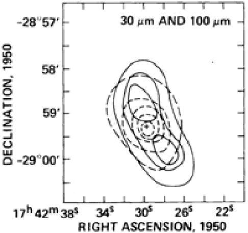
Figure 1.1: High angular resolution far IR continuum observations of the galactic centre (Becklin et al., 1982). The 30$\mu$m map (dashed) superimposed on 100$\mu$m (solid) contours that outline the CND’s lobes.

The CND was first observed in IR continuum emission from dust at 30, 50 and 100$\mu$m using the 1 metre diameter Kuiper airborne observatory. The CND appeared as two lobes that were symmetrically located to the NE and SW about a relatively dust-free central cavity in 100$\mu$m emission with some 30$\mu$m emission close to the galactic centre (see Fig. 1.1). The symmetry and orientation of the lobes suggested a ring like structure with a major axis approximately aligned with the galactic plane (Becklin et al., 1982).

This chapter outlines the currently known information about the CND from observations spanning some 25 years including two reviews, the first summarises earlier work up to 1989 (Genzel, 1989), the second written last year covers more recent research (Genzel et al., 2010). It closes with discussion of questions posed by its existence and an outline of this thesis’ structure.

1.2 Current Status

Observations of CO, CS and HCN subsequently led to the discovery of the CND rotating about the galactic centre (Serabyn and Lacy, 1985; Serabyn et al., 1986; Guesten et al., 1987). The disk was found to have an inner radius of 1.5 to 1.7pc and extend to 5pc in HCN and $>$7pc in CO (Guesten et al., 1987), and more recent observations have detected HCN out to 7pc and CO up to 9pc from the galactic centre. (Christopher et al., 2005; Oka et al., 2007, 2011).

The disk is composed of clumps (cores), with diameters from 0.14 to 0.43 pc, rotating in a number of kinematically distinct streamers about the galactic centre (Guesten et al., 1987; Jackson et al., 1993). The disk’s major axis is aligned to a position angle of $\sim$ 25^∘ and inclination of $\sim$ 70^∘ to the plane of the sky. (Serabyn et al., 1986; Jackson et al., 1993; Marshall et al., 1995). It was noted that the rotation was perturbed in several ways with a large local velocity dispersed throughout the disk. The position angle changed with radius and in inclination with azimuthal angle, i.e. the disk was warped. The perturbations together with the disk’s clumpiness indicated a non-equilibrium configuration with a short age of a few orbital periods (Guesten et al., 1987).

The ring’s rotational velocity is $\sim$110 km s^-1 between 2 to 5pc from the galactic centre (see Fig. 1.4). Lower velocities are indicated by CII and CO(7-6) at radii $\geq$ 4pc and higher velocities, 130–140 km s^-1, are indicated by HCN in the North Eastern part of the ring at 2pc (Guesten et al., 1987). Marshall et al. (1995) fitted a 3D rotating ring model to HCN (4-3) and (3-2) data and inferred a flat velocity profile, while noting that Harris et al. (1985) showed a velocity fall off between 2 and 6 pc from the centre with CO observations.

The disk has been interpreted as an accretion disk transferring material from the giant molecular clouds located in the region 10–30pc from the galactic centre to the cavity located inside the the inner radius of the ring (Guesten et al., 1987; Oka et al., 2011) (see Fig. 1.2). Parts of the disk’s inner radius located in the East, North and West were found to be associated with the arms of the mini-spiral SgrA West that was suggested from the observations of line broadening of HCN(4-3) core line spectra, possibly caused by a transient turbulent cascade of material falling towards the central cavity, in locations where they overlap, at least in projection, the mini-spiral arms (Montero-Castaño et al., 2009). Christopher et al. (2005) also noted a number of interactions between the ionised gas in the ring’s inner radius and the western arc of the mini-spiral, which is both spatially and kinematically consistent with the CND’s inner radius material. They also suggested a possible connection between the northern arm of the mini-spiral and the North Eastern extension of the CND (see Fig.1.3).

The Northern and Southern lobes of the CND have different excitation levels and densities with the Southern warmer and denser than the Northern part. NH₃ (6-6) data confirm that molecular gas in the ring is denser and colder than the molecular gas in the cavity (Montero-Castaño et al., 2009). The South Eastern portion of the ring is denser than the South Western part of the CND with the SE part becoming warmer and more diffuse as material heads NW approaching the central super massive black hole. The difference between the HCN(4-3) and NH₃(6-6) data indicates a probable infall of material from the CND toward the galactic centre through the Eastern part of the ring structure (Montero-Castaño et al., 2009).

Herrnstein and Ho (2002) inferred that material inside the ring is hotter and denser than the mini spiral and appears unrelated, this seems at odds with the conclusions of Christopher et al. (2005) and Montero-Castaño et al. (2009) who infer a connection. NH₃(3-3) emission suggested an interaction between the southern arm of the mini-spiral and the southernmost part of the CND, with material in the ring undergoing compression as the arm approaches the CND before spiralling inward to the centre. The inner edge of the CND is more highly excited than the outer part of the ring most probably due to the stellar cluster, inside, exciting the ring’s inner edge (Montero-Castaño et al., 2009).

Core size estimates have varied from 0.05 to 0.12pc by (Jackson et al., 1993) who used a telescope with a beam size incapable of resolving the core images, to 0.14 to 0.43pc (Christopher et al., 2005) and 0.14 to 0.5pc (Montero-Castaño et al., 2009), with the larger core sizes based on resolved images.

The dust continuum emission is well approximated by thermal emission at 20, 60 and 100 K. Observations by Mezger et al. (1989) showed that warm dust $\geq$60 K accounts for only $\sim$10% of the total dust mass in the CND and is located near the ionisation front of SgrA West. The remaining dust in the disk appears to be rather cold at $\sim$20 K. The south-western edge of the ring of dust surrounding SgrA East and the southern lobe of the CND overlap. Both have similar clumpy density structures but different radial velocities which allow them to be separated by observations of optically thin molecular lines (Mezger et al., 1989).

Etxaluze et al. (2011) found the spectral energy distribution for the far IR emission from dust in the CND was best represented by a continuum summing dust temperatures at 90, 44.5 and 23 K with the cold component accounting for $\sim$ 3.2$\times$10⁴ M_⊙ out of the estimated total $\sim$5$\times$10⁴ M_⊙ in the central 2pc of the CND and is similar to the findings of Mezger et al. (1989).

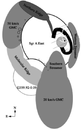
Figure 1.2: Schematic drawing of the central 10pc of the Milky Way Galaxy as seen in the plane of the sky (Herrnstein and Ho, 2002). The CND is shown as a solid black torus, G359.92-0.09 is an adjacent Supernova Remnant to SgrA East. The central black hole is shown as a black dot.

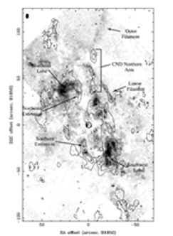
Figure 1.3: HCN emission in contours superimposed on a reverse grey scale H₂(1-0)S($1$)line emission map (Christopher et al., 2005). Significant features in both H₂ and HCN emission are labelled, and SgrA^∗ is marked by a circle at(0,0).

Figure 1.4: Flux weighted average velocity map of the HCN(1-0) emission in colour with integrated emission (black contours) Christopher et al. (2005). Blue colour indicates emission with negative velocities moving towards, red colour emission with positive velocities moving away from the observer and showing the disk’s rotation. Velocities are relative to V_LSR = 0 km s^-1 with magnitudes indicated by colour bar to the right of the map. Offsets are relative to SgrA^∗ at (0,0).

1.3 Motivation for this Study

After twenty-five years of observing the CND there remains considerable uncertainty as to the molecular density of the CND’s cores. Genzel et al. (2010) summarises the position by describing the two prevailing scenarios as

1. the original view of less dense (10⁶cm^-3) warm gas ($>$ 100 K) cores which are tidally unstable leading to a transient lifetime of $\sim$10⁵ yr, or

2. the more recent idea of a denser (10⁷-10⁸ cm^-3) cool gas (50-100 K) which provides stable cores with long lifetimes $\sim$10⁷yr, that is long enough for the opportunity for star formation from core condensation.

Evidence for the first scenario includes that there is no recorded evidence of precession of the orbits of the inner stellar cluster which would be expected if the CND’s mass is 10⁶ M_⊙. Šubr et al. (2009) also noted that gravitational torque would have destroyed the central disk of young massive stars, inside the CND, within its age of 6 Myr. Infra-red emission from the dust in the CND has the characteristics of an optically thin medium and is further evidence for scenario one. For an optically thick medium (scenario two) cores would appear as dark spots in an infra-red image (Mezger et al., 1996). To date there have been no recorded observations of such dark spots and Scenario two relies on the size and density of the cores to provide stability against tidal forces and long lifetimes.

Large Velocity Gradient (LVG) modelling of CS(2-1), (3-2) and (5-4) transitions determined 10⁶cm^-3 as the upper limit of molecular hydrogen density (Serabyn et al., 1989); this is the same density proposed by Jackson et al. (1993). Marr et al. (1993) proposed a density of 2$\times$10⁶ cm^-3 for an optically thick ($\tau$=4) HCN(1-0) transition at a kinetic temperature of 250 K. Christopher et al. (2005) proposed a typical density of 3-4 $\times$ 10⁷cm^-3 for an average core diameter of 0.25pc with a kinetic temperature of 50 K and optically thick ($\tau$=4) HCN. Montero-Castaño et al. (2009) argued for virially stable cores based on HCN(4-3) data combined with HCN(1-0) Christopher et al. (2005) data scaled to match. These papers show examples of both scenarios 1 & 2 and indicate the need for further testing of the value for the hydrogen density in the CND.

The present thesis attempts to resolve the density question through LGV modelling of the HCN(1-0), (3-2) and (4-3) transitions together with the HCO⁺(1-0) transition. Two sets of cores that are considered spatially and kinematically matched are presented in the analysis. The first set of cores are taken from Marr et al. (1993) for the (1-0) transition of H¹²CN, H¹³CN and HCO⁺ combined with the HCN(3-2) transition. The second set uses data for HCN(1-0) and HCO⁺(1-0) (Christopher et al., 2005), for HCN(3-2) (Jackson et al., 1993) and for HCN(4-3) (Montero-Castaño et al., 2009). The first set is not resolved, however the transitions were scaled to a common resolution and hence is spatially and kinematically matched for all five cores. The second set consists of data from three sources with resolved data for the HCN(1-0) and (4-3) transitions and unresolved data for the HCN(3-2) transition which is corrected by a filling factor (based on the average core size of Christopher et al. (2005)) to provide brightness temperature comparable with those for the resolved transitions.

LVG modelling for all transitions is carried out for a range of hydrogen densities and molecule column densities. The results favour an optically thin HCN and hence lower hydrogen density than advocated by Christopher et al. (2005) and Montero-Castaño et al. (2009).

1.4 Thesis Outline

Chapter 2 outlines the radiative transfer equation and the equations describing emission and absorption, incorporating the Einstein A and B coefficients, optical depth, intensity, integrated intensity, excitation temperature, brightness temperature and collisions, which are used in the model for tracing molecular rotational excitation from collisions with molecular hydrogen. The molecular excitation model that is used to analyse the observed results is then described briefly.

Chapter 3 uses the positions and velocities of twenty-six cores identified by Christopher et al. (2005) to check the orientation of the disk’s plane relative to the plane of the sky. The positions of each core in the plane of the sky are converted to deprojected (true) offsets (from SgrA^∗) in the disk’s plane. Model core radial velocities were calculated for the adopted disk orientation of PA = 25^∘ and inclination = 60^∘ and are then compared with the observed core velocities. The locations and radial velocities of OH masers (Sjouwerman and Pihlström, 2008) and water and methanol masers (Yusef-Zadeh et al., 2008) in and around the CND are also explored to assess their relationship to the disk. Two groups of cores are then identified as having consistent spatial and kinematic properties and selected for modelling. Five cores from Marr et al. (1993) were chosen as the first group and seven cores from Jackson et al. (1993) and Montero-Castaño et al. (2009) that can be co-located with Christopher et al. (2005) cores form the second. Four cores from Marr et al. (1993) are found to be co-located with members of the second group of seven cores

Chapter 4 describes the input parameters for the modelling, along with the results. The results indicate that the molecular hydrogen gas number density n(H₂) $\sim$ 10⁶ cm^-3 agrees with scenario 1, with optically thin, inverted HCN(1-0) and HCO⁺(1-0) transitions. Core densities are consistent with the Christopher et al. (2005) optically thin scenario and as a consequence the cores are transient with little or no prospect of star formation from their condensation. The mass of the CND is also an order of magnitude less than the estimated 10⁶ M_⊙.

Chapter 5 summarises the thesis results and conclusions, areas for future study are also identified.

Chapter 2 Molecular Excitation, Line Formation and Radiative Transfer

2.1 Introduction

This chapter outlines the radiative processes and their equations used to describe the radiative transfer process, particularly as it applies to emission arising from molecular rotation of tracers colliding with molecular hydrogen.

Section 2.2 describes the instantaneous emission, absorption and collision processes which are associated with emission and absorption of photons from a material illustrated by Fig. 2.1. The Equation of Radiative Transfer which describes how radiative intensity changes as radiation travels along a path through a medium with a known optical depth is then developed in Section 2.3. Section 2.4 follows explaining how the background radiation components are incorporated into radiative transfer equation.

Section 2.5 explains how brightness temperature, which is an alternative measure of intensity, is used in the LVG model. Integrated Intensity, which is the total radiation emitted by the medium and is the sum of intensities across the width of the spectrum, is then described in Section 2.6.

The programme Molex, which was written by M. Wardle and modified by J. Chapman, that is used in this thesis to analyse the HCN observations reported in the published papers under review is described in the closing Section 2.7. The programme is based on the Large Velocity Gradient model (e.g. Section 14.10 of Rohlfs and Wilson (2006)). The model does not rely on the gas being in Local Thermal Equilibrium (LTE) and assumes that changes in local velocity predominate over thermal broadening of spectral lines. The probability of an emitted photon escaping the source is included in the radiative transfer equations for estimating the line intensities and optical depths of the radiating material. The model commonly assumes a spherical escape model and a Gaussian velocity profile but can cater for other escape models and velocity profiles.The adoption of an escape probability simplifies the analysis of the radiation transferred and promotes faster convergence to a solution of each calculation of the many energy transition levels of the trace molecule.

The HCN transitions of interest in this thesis are (1-0), (3-2) and (4-3). The (1-0) transition level observations of HCO⁺ and H¹³CN are also analysed. The calculations were checked using Radex, a similar programme to Molex. Radex is accessible on the web , for calculations for static conditions of a species using the underlying equations for this LVG model as outlined in van Langevelde and van de Tak (2004). More recently a version of the programme has become available in the public domain for download. Radex is also described in a more recent paper written by van der Tak et al. (2007).

2.2 Absorption and Emission Coefficients

The radiation intensity from a source for a simple case is a balance between emission and absorption of photons by the source. Collisions within the source also contribute indirectly to the intensity by excitation and de-excitation which change level populations. These processes are illustrated in Fig. 2.1 and described in the following sub-sections.

Figure 2.1: Transitions between two energy levels E₁ and E₂ above ground level with the statistical weights of the levels g₁ and g₂ and n₁ and n₂ molecules per unit volume. A₂₁ is the Einstein A probability coefficient for downward spontaneous transition from an upper to lower level; B₂₁ is the Einstein probability coefficient for stimulated emission; B₁₂ is the Einstein coefficient for absorption; U_ν is the energy density for photons per unit frequency interval; C₂₁ is the rate coefficient for de-excitation from level 2 to level 1 by collisions and C₁₂ is the rate coefficient for excitation from level 1 to level 2

2.2.1 The Spontaneous Emission Coefficient j_ν

The spontaneous emission coefficient of isotropically emitted photons is given by the expression

$$j_{\nu}=\frac{n_{2}A_{21}}{4\pi}h\nu\,\phi(\nu)\,,$$ (2.1)

where n₂ is the population of the upper level 2, of a transition, A₂₁ is the Einstein A probability coefficient of emission (see Fig. 2.1), h is Planck’s constant, $\nu$ is the frequency of the emission of the nominated transition between an upper and lower level and $\phi(\nu)$ is the line function describing the shape of the spectral line centred on the frequency $\nu_{0}$, (e.g. a Gaussian) and can be defined as

$$\int_{0}^{\infty}\!\phi(\nu-\nu_{0})\,\mathrm{d}\nu=1\,.$$ (2.2)

The intensity of emission at frequency $\nu$, I_ν, can be expressed as the integral of the emission coefficient along a path, ds, through the medium (if it is optically thin) as

$$I_{\nu}=\int\!j_{\nu}\,\mathrm{ds}$$ (2.3)

so that the line integrated emission I is given by the expression

$$I=\int I_{\nu}\,\mathrm{d}\nu$$ (2.4)

and substituting for I_ν from Eqn. 2.3 gives

$$I = \int_{line}\left(\int\!\frac{\mathrm{n}_{2}A_{21}}{4\pi}h\nu_{21}\phi(\nu)\,\mathrm{d}s\right)\,\mathrm{d}\nu$$ (2.5)

$$= \int_{line}\frac{A_{21}}{4\pi}h\nu_{21}\phi(\nu)\left(\int\mathrm{n}_{2}\,\mathrm{d}s\right)\,\mathrm{d}\nu\,,$$ (2.6)

where n₂ is the population of the transition’s upper level which when integrated along the emission’s path through the medium produces the total column density, N₂ in the upper level. The line function, $\phi(\nu)$, is assumed independent of the distance,s, through the medium.

The column density, N_mol, in all levels of the molecule is related to N₂ by

$$N_{2}=N_{\mathrm{mol}}\times\mathrm{x}_{2}$$ (2.7)

where x(2) is the fraction of the total population in the upper level Eqn. 2.5 then becomes

$$I = \frac{h\nu_{21}}{4\pi}A_{21}N_{2}\int\phi(\nu)\,\mathrm{d}\nu,$$ (2.8)

$$I = \frac{h\nu_{21}}{4\pi}A_{21}N_{\mathrm{mol}}x(u).$$ (2.9)

2.2.2 Absorption Coefficient $\alpha_{\nu}$

Optical depth, $\tau_{\nu}$ , is defined as the integration of the absorption coefficient $\alpha_{\nu}$ over the depth, ds, of the radiation field as follows

$$\tau_{\nu}=\int\alpha_{\nu}\,\mathrm{d}s\,,$$ (2.10)

where $\alpha_{\nu}$, the coefficient of absorption is defined by

$$\alpha_{\nu}=(n_{1}B_{12}-n_{2}B_{21})h\nu\phi(\nu)\,,$$ (2.11)

and n₂ and n₁ are the upper and lower level populations, B₁₂ is the Einstein B probability coefficient for absorption and B₂₁ the Einstein probability coefficient for stimulated emission, (see Fig. 2.1)

Using the relationship

$$g_{1}B_{12}=g_{2}B_{21}$$ (2.12)

where g₁ and g₂ are the statistical weights of the transition states and

$$A_{21}=\frac{2h\nu^{3}}{c^{2}}B_{21}\,;$$ (2.13)

substituting into the expression for $\alpha_{\nu}$ produces

$$\alpha_{\nu}=\frac{A_{21}}{8\pi}\frac{c^{2}}{\nu^{2}}\left(\frac{n_{1}g_{2}}{g_{1}}-n_{2}\right)\phi(\nu)\,;$$ (2.14)

and further substituting x${}_{1}n_{\mathrm{tot}}$ for $n_{1}$ and x${}_{2}n_{\mathrm{tot}}$ for $n_{2}$, where x₁ and x₂ are the fractions of the total population n_tot produces,

$$\alpha_{\nu}=\frac{A_{21}}{8\pi}\frac{c^{2}}{\nu^{2}}n_{\mathrm{tot}}\left(\frac{x_{1}g_{2}}{g_{1}}-x_{2}\right)\phi_{\nu}\,.\\$$ (2.15)

Integrating with respect to $\mathrm{ds}$ gives

$$\tau_{\nu} = \int\alpha_{\nu}\,\mathrm{d}s$$ (2.16)

$$= \frac{A_{21}}{8\pi}\frac{c^{2}}{\nu^{2}}\left(\frac{x_{1}g_{2}}{g_{1}}-x_{2}\right)\phi(\nu)\int n_{\mathrm{tot}}\,\mathrm{d}s\,.$$ (2.17)

Using the relationships

$$\frac{\mathrm{d}\nu}{\nu}=\frac{\mathrm{d}v}{c}$$

and

$$\phi(\nu)\mathrm{d}\nu=\phi(\mathrm{v})\mathrm{dv}$$

where $\phi(\nu)$ is the frequency line profile, $\mathrm{d}\nu$ a small interval in line frequency, $\phi$(v) is the velocity line profile and $\mathrm{dv}$ a small interval in line velocity implies that,

$$\phi(\nu)=\phi(\mathrm{v})\frac{\mathrm{dv}}{\mathrm{d}\nu}=\phi(\mathrm{v})\frac{\mathrm{c}}{\nu}$$

and so

$$\tau_{\nu}=\frac{A_{21}c^{3}}{8\pi\nu^{3}}\left(\frac{x_{1}g_{2}}{g_{1}}-x_{2}\right)N_{\mathrm{mol}}\phi(v)\,.$$ (2.18)

The optical depth at the line centre of a Gaussian line profile is calculated from the expression

$$\phi(\mathrm{v})=\frac{1}{\sqrt{2\pi}\sigma_{\mathrm{v}}}\exp\left(-\frac{\mathrm{v}^{2}}{2\sigma_{\mathrm{v}}^{2}}\right)$$ (2.19)

where $\sigma_{\mathrm{v}}$ is the standard deviation of the Gaussian. To relate the FWHM velocity $\Delta\mathrm{v}$ to $\sigma_{\mathrm{v}}$ the following expression is evaluated for the FWHM line width value, $\phi(\mathrm{v})$ = $\frac{1}{2}$ for a curve with central value = 1.

$$\exp\left(-\frac{(\Delta V/2)^{2}}{2\sigma_{V}^{2}}\right)=\frac{1}{2}$$ (2.20)

so that

$$\sigma_{v}=\frac{\Delta V}{2\sqrt{2\mathrm{ln}2}}\,.$$ (2.21)

At the line centre the value of the line profile $\phi$(0) is

$$\phi(0)=\frac{1}{\sqrt{2\pi}\sigma_{v}}=2\sqrt{\frac{\mathrm{ln}2}{\pi}}\left(\frac{1}{\Delta V}\right)\,,$$ (2.22)

so that by substituting Eqn. 2.22 into Eqn. 2.18, the optical depth at line centre $\tau_{0}$ is

$$\tau_{0}=2\sqrt{\frac{\mathrm{ln}2}{\pi}}\frac{A_{21}}{\Delta V}\frac{\lambda^{3}N_{mol}}{8\pi}\left(x_{1}\frac{g_{2}}{g_{1}}-x_{2}\right)\,.$$ (2.23)

2.2.3 Collisions

The number of effective collisions between two particles A and B per unit volume is given by

$$\mathrm{n_{A}}\mathrm{n_{B}}\sigma\mathrm{(v)V}$$

where n_A and n_B are number densities of each in cm^-3, $\sigma$(v) is the collisional cross section (which depends on the energy level of the incoming particles) and V is the velocity of the incoming particles in cm s^-1

The collision rate $\gamma$ for a Maxwellian velocity distribution of moving particles at temperature T is given by the expression

$$\large{\gamma}\normalsize_{AB}=n_{A}n_{B}\int^{\infty}_{0}V\sigma(\mathrm{v})4\pi V^{2}\Big{(}\frac{m}{2\pi kT}\Big{)}^{\frac{3}{2}}\exp\left(-\frac{mV^{2}}{2kT}\right)\mathrm{d}V\,;$$ (2.24)

for a large number of collisions and applying the principle of detailed balance the following equation applies

$$\frac{\gamma_{12}}{\gamma_{21}}=\frac{g_{2}}{g_{1}}\exp-\left(\frac{\mathrm{E}_{21}}{\mathrm{kT}}\right)\,.$$ (2.25)

Collision rates are used in Molex to calculate the populations for the range of transition levels of the rotating trace molecules colliding with molecular hydrogen in the CND. The collision rates for all transitions at a range of specific temperatures are included in the molecular properties data file input to Molex. Molex uses an extrapolation routine to calculate collision rates for the kinetic temperature of the molecule to be modelled.

The population of a series of levels $j=1,2,3,4\cdots$ is determined by the rates of collisional and radiative excitation and de-excitation between the levels (see Fig. 2.1).

Changes in all levels of the molecule contribute to changes in the population of level j according to

$$\begin{split}\dfrac{\mathrm{d}n_{j}}{\mathrm{d}t}=\sum_{k>j}A_{kj}n_{k}+\sum_{k<j}(B_{kj}U_{kj}n_{k}-B_{jk}U_{kj}n_{j})+\sum_{k>j}(C_{kj}n_{k}-C_{jk}n_{j})\\ -\sum_{i<j}A_{ji}n_{j}+\sum_{i<j}(B_{ij}U_{ji}n_{i}-B_{ji}U_{ji}n_{j})+\sum_{i<j}(C_{ij}n_{i}-C_{ji}n_{j})\end{split}$$ (2.26)

$$\begin{split}=\sum_{k>j}\left[A_{kj}n_{j}+B_{kj}U_{kj}\left(n_{k}-\dfrac{g_{k}}{g_{J}}n_{j}\right)\right]-\sum_{i<j}\left[A_{ji}n_{j}+B_{ji}U_{ji}\left(n_{j}-\dfrac{g_{j}}{g_{i}}n_{i}\right)\right]\\ +\sum_{k>j}(C_{kj}n_{k}-C_{jk}n_{j})+\sum_{i<j}(C_{ij}n_{i}-C_{ji}n_{j})\,.\\ \end{split}$$ (2.27)

U_kj and U_ji are the radiation densities integrated over their respective levels kj and ji and defined as,

$$U_{ji}=\int\phi_{ji}(\nu)U_{\nu}\mathrm{d}\nu\,,$$ (2.28)

where U_ν, the energy density for photons per unit frequency interval is,

$$U_{\nu}=\dfrac{1}{c}\int I_{\nu}\mathrm{d}\Omega\,.$$ (2.29)

Assuming full redistribution, so that the one dimensional velocity distribution function is the same Maxwellian for all transitions, then

$$\phi_{ji}(\nu)=\dfrac{\lambda_{ji}}{(2\pi)^{1/2}\sigma}\mathrm{exp}(-v^{2}/2\sigma^{2})$$ (2.30)

where

$$\sigma=(kT/m)^{1/2}$$ (2.31)

and

$$v=-(\nu-\nu_{ij})c/\nu_{ij}\,.$$ (2.32)

The flux from the transition j to i can then be defined as

$$F_{ji}=\dfrac{B_{ji}U_{ji}}{A_{ji}}=\dfrac{c^{2}}{2h\nu^{3}}\int\phi_{ji}I_{\nu}\mathrm{d}\nu\dfrac{\mathrm{d}\Omega}{4\pi}$$ (2.33)

where the integral is the angle-averaged intensity, J_ν, integrated over the line profile. The radiation field is determined by the radiative transfer Eqn. 2.41. The energy density U_ν enters Eqn. 2.26 as the level populations determine the emission and absorption coefficients j_ν and $\alpha_{\nu}$.

While it is very difficult to simultaneously solve the equations for statistical equilibrium and radiative transfer in the general case it can be done for simple geometries as follows. Any transition 2 $\rightarrow$ 1 contributes

$$A_{21}\left[n_{2}+F_{21}\left(n_{2}-\dfrac{g_{2}}{g_{1}}n_{1}\right)\right]$$ (2.34)

positively to $\mathrm{d}n_{1}/\mathrm{d}t$ and negatively to $\mathrm{d}n_{2}/\mathrm{d}t$. For a spatially uniform source function $S_{\nu}=j_{\nu}/\alpha_{\nu}$,

$$I_{\nu}=I_{0}e^{-\tau_{\nu}}+S_{\nu}(1-e^{-\tau_{\nu}})\,.$$ (2.35)

For full redistribution in the absence of overlapping lines $S_{\nu}=B_{\nu}(T_{ex})$ and does not change significantly over the line, this usually true for the background radiation I₀ so that

$$F_{21} = \frac{c^{2}}{2h\nu^{3}}\left[S_{\nu}+(I_{0}-S_{\nu})\int\phi_{21}e^{-\tau_{\nu}}\mathrm{d}\nu\dfrac{\mathrm{d\Omega}}{4\pi}\right]$$ (2.36)

$$= \frac{c^{2}}{2h\nu^{3}}\left[\beta_{21}I_{0}+(1-\beta_{21})S_{\nu}\right]\,.$$ (2.37)

$$\beta_{21}=\int\phi_{21}e^{-\tau_{\nu}}\mathrm{d\nu}\dfrac{\mathrm{d\Omega}}{4\pi}$$

is the escape probability and in this case the contribution to $\mathrm{d}n_{1}/\mathrm{d}t$ is

$$\beta_{21}A_{21}n_{2}+\dfrac{c^{2}}{2h\nu^{3}}I_{0}\left(n_{2}-\dfrac{g_{2}}{g_{1}}n_{1}\right)\beta_{21}A_{21}.\\$$ (2.39)

The escape probability for a sphere has been adopted for the analysis performed in this thesis and in Molex to calculate $\beta$ where the absolute value of $\tau>0.001$ in Molex and for a radius of $\tau/2$ the escape probability is

$$\beta=\frac{1.5}{\tau}\left(1-\frac{2}{\tau^{2}}+\left(\frac{2}{\tau}+\frac{2}{\tau^{2}}\right)e^{-\tau}\right)$$ (2.40)

which reduces to $\frac{1.5}{\large{\tau}}$ under optically thick conditions.

2.3 The Radiative Transfer Equation

The radiative transfer equation relates the change in intensity along a path to the net effect of spontaneous emission and absorption. It is given by

$$\frac{dI_{\nu}}{\mathrm{ds}}=-\alpha_{\nu}I_{\nu}+j_{\nu}$$ (2.41)

where $\alpha_{\nu}$ is the absorption coefficient, j_ν is the spontaneous emission coefficient, I_ν is the intensity and ds is the distance along the radiation’s path through the medium.

Optical depth in the differential form of Eqn. 2.10 is

$$\mathrm{d}\tau_{\nu}=\alpha_{\nu}\mathrm{ds}$$ (2.42)

and dividing Eqn. 2.41 by $\alpha_{\nu}$ leads to

$$\frac{\mathrm{d}I_{\nu}}{\mathrm{d}\tau_{\nu}}=-I_{\nu}+S_{\nu}$$ (2.43)

where the source function is

$$S_{\nu}=\frac{j_{\nu}}{\alpha_{\nu}}\,.$$ (2.44)

Transposing the terms of Eqn. 2.43 and multiplying by e${}^{\tau_{\nu}}$ gives

$$\left(I_{\nu}+\frac{\mathrm{d}I_{\nu}}{\mathrm{d}\tau_{\nu}}\right)e^{\tau_{\nu}}=S_{\nu}e^{\tau_{\nu}};$$ (2.45)

the expression on the left hand side (LHS) is $\dfrac{\mathrm{d}}{\mathrm{d}\tau}\left(I_{\nu}e^{\tau_{\nu}}\right)$ so that integrating with respect to $\tau_{\nu}$ produces

$$\left[I_{\nu}e^{\tau_{\nu}^{{}^{\prime}}}\right]_{0}^{\tau_{\nu}}=\int_{0}^{\tau_{\nu}}\!S_{\nu}e^{\tau_{\nu}^{{}^{\prime}}}\ \mathrm{d}\tau_{\nu}^{{}^{\prime}}$$ (2.46)

and assuming that $S_{\nu}$ is constant,

$$I_{\nu}=I_{0}e^{-\tau_{\nu}}+S_{\nu}(1-e^{-\tau_{\nu}})$$ (2.47)

where $I_{0}=I_{\nu}$ at $\tau_{\nu}=0$  .

The first and second terms on the right hand side (RHS) of Eqn. 2.47 are the contributions of the background radiation and emission from within the medium , correspondingly corrected for optical depth.

The radiative transfer equation is a central part of the calculation of intensities in Molex, and S_ν depends on the molecular excitation discussed in Section 2.2.3.

2.4 Background Radiation

Background radiation arises from two sources :

1. the cosmic microwave background, CMB, at the relevant frequency calculated from the Planck function

   $$I_{\mathrm{CMB}}=B_{\nu}(T_{\mathrm{CMB}})=\dfrac{2h\nu^{3}/c^{2}}{(\exp(h\nu/kT_{\mathrm{CMB}})-1)}$$ (2.48)

   where $T_{\mathrm{CMB}}=2.728\,\mathrm{K}$, and
   

2. IR radiation from the irradiation of the CND’s dust by sources located in the central cavity which is surrounded by the CND. The contribution of external dust radiation is calculated from

   $$I_{\mathrm{dust}}=B_{\nu}(T_{\mathrm{dust}})(1-\exp(-\tau_{\mathrm{dust}}))\,,$$ (2.49)

   where T_dust is the dust temperature and $\tau_{\mathrm{dust}}$ is the dust’s optical depth.

The total background radiation, I₀, is the sum of the contribution from these background sources. The LVG model subtracts the background radiation (I₀) from total radiation to provide a radiation intensity for comparison with the gas core intensities. This given by

$$I_{\nu}-I_{0}=S_{\nu}(1-e^{-\tau})+I_{0}e^{-\tau}-I_{0},$$ (2.50)

which reduces to

$$I_{\nu}-I_{0}=\left(S_{\nu}-I_{0}\right)\left(1-e^{-\tau}\right)\,,\\$$ (2.51)

where the LHS of Eqn. 2.51 represents the net intensity at line centre.

The effect of dust in the LVG model is taken into account by specifying total extinction in the V filter band (Av) and temperature (T_dust). Av depends on the dust’s optical depth and temperature that Marr et al. (1993) assumed to be 75 K and together with the observed intensity of $2.0\times 10^{5}$ M Jys^-1 at 100$\mu$m (both estimates inferred from Becklin et al. (1982)) allowed calculation of the dust’s optical depth using,

$$I_{\mathrm{dust}}=\large{\tau}\normalsize_{\mathrm{dust}}\times B_{\nu}(T_{\mathrm{dust}})\,,$$ (2.52)

where B_ν is calculated using the Planck equation for T_dust = 75 K and $\lambda$ = 100$\mu$m. The result, $\tau_{\mathrm{dust}}=3.43\times 10^{-2}$ that is consistent with the use of the optically thin expression in Eqn. 2.52 and also with the estimates of Becklin et al. (1982) who found that the mean optical depth over their map(Fig. 1(c)) was 0.05 and the value at the position of the galactic centre was $\backsim 0.03$.

Av is related to the dust’s optical depth ($\tau_{\mathrm{dust}}$) and the column density for neutral hydrogen (N_H) substituting typical values of N_H = 5.8$\times$10²¹ E(B-V) cm^-2 mag^-1 (Bohlin et al., 1978), $\tau_{\mathrm{v}}$ = 0.4$\ln$ 10 Av (Lockett and Elitzur, 1989) and Av = 3.1 E(B-V) (Rieke and Lebofsky, 1985) into the relationship between the dust optical depth and extinction was established from an adopted fit of the total graphite and silicate extinction curve in . 9 of Draine and Lee (1984) produces,

$$\large{\tau}\normalsize_{\mathrm{dust}}=12.769f_{x}\lambda^{\!-2}\mathrm{Av}\,,$$ (2.53)

where

$$f_{x}=-11.478+20.1769x-12.2355x^{2}+3.2809x^{3}-0.33010654x^{4}\,,$$ (2.54)

is a polynomial fit to the extinction curve (M. Wardle, private communication) and

$$\mathrm{x}=\mathrm{log}_{10}\lambda(\mu\mathrm{m})\,.$$ (2.55)

Eqn. 2.53 is valid for $30\mu\mathrm{m}<\lambda<1000\mu\mathrm{m}$, for longer wavelengths $f_{x}=1$ and entering $3.43\times 10^{-2}$ into Eqn. 2.53 for $\tau_{dust}$ gives a value of Av = 26.9 which is used in Molex.

2.5 Brightness Temperature

The brightness temperature B_ν(T_b) (the equivalent black body radiation from a source at temperature T) is usually derived from the Planck function

$$B_{\nu}(T_{b})=I_{\nu}$$ (2.56)

however in the millimetre and sub millimetre wavelength ranges, the brightness temperature is frequently defined as

$$T_{b}(RJ)=\frac{\lambda^{2}}{2\mathrm{k}}I_{\nu},$$ (2.57)

where T_b(RJ) is the brightness temperature which is the intensity based on the Rayleigh-Jeans approximation to the Planck function where h$\nu$ $\ll$ kT. In this equation $\lambda$ is the radiation’s wavelength, k is the Boltzmann constant and I_ν is radiation’s intensity. This relationship is used at sub mm wavelengths where it does not strictly apply but corresponds to observer conventions. The peak brightness temperature at line centre is T_b(0) where the shorthand version T_b will be used and is the value of the temperature used in the model to match the observed brightness temperatures in Chapter 4.

2.6 Integrated Intensity

Molex calculates integrated intensity by using the line’s wavelength ($\lambda$), Einstein A coefficient (A₂₁), HCN column density (N_HCN), upper level population (x_u) and escape probability ($\beta$).

The equation is derived as follows from the definition:

$$\int I_{\nu}\,\mathrm{d}\nu=2k\frac{\nu^{2}}{c^{2}}\int T_{b}\,\mathrm{d}\nu\,,$$ (2.58)

and using the relationship

$$\frac{\mathrm{d}\nu}{\nu}=\frac{\mathrm{d}V}{c}\,,$$

the RHS of Eqn. 2.58 can be integrated with respect to $\mathrm{d}\nu$ :

$$\int I_{\nu}\,\mathrm{d}\nu=2k\frac{\nu^{2}}{c^{2}}\frac{\nu}{c}\int T_{b}\,\mathrm{d}V$$ (2.59)

so that

$$\int T_{b}\,\mathrm{d}V=\frac{c^{3}}{2k\nu^{3}}I_{\nu}\,.$$ (2.60)

Substituting the intensity from Eqn. 2.8 and adjusting for the likelihood of re-absorption using the escape probability term $\beta$ Eqn. 2.60 becomes:

$$\int T_{b}\,\mathrm{d}V=\frac{c^{3}}{2k\nu^{3}}\frac{h\nu_{21}}{4\pi}A_{21}N_{\mathrm{mol}}x_{u}\beta\,.$$ (2.61)

This reduces to

$$\int T_{b}\,\mathrm{d}V=\frac{hc\lambda^{2}}{8\pi}A_{21}N_{\mathrm{mol}}x_{u}\beta\,,$$ (2.62)

which is used in Molex expressed in units of K km s^-1.

2.7 The Molex Programme

Molex uses one of a number of molecular data files from the Cologne Data Base for Molecular Spectroscopy that contains details of transition frequencies, Einstein A coefficients and collision rates for a range of gas temperatures for all the molecule’s transitions. Data from a second input file prepared by the user specifies the molecule and the transitions to be analysed, the kinetic temperature of the gas, the dust temperature, dust Av extinction, the fraction of molecular hydrogen in ortho form (0.75), the initial and final hydrogen densities along with the step interval, and the initial, final and step intervals for the column density of the rotating trace molecule.

The programme starts at a point where the HCN molecule is in a state of LTE and operates in specified steps of decreasing hydrogen number density and increasing HCN column density to cover the range of interest. Level populations are calculated along with escape probabilities for all levels to produce intensities, opacities and brightness for the gas temperatures. This author used $10^{12}$ as the starting value for both the HCN column density and atomic hydrogen number density to ensure initial LTE conditions. Log column densities were then incrementally increased from 12 to 18 for each increment of log hydrogen densities which is decreased from 12 to 3, increments of 0.1 are specified for both densities.

Selected output parameters, notably the brightness temperature T_b and optical depth $\tau$ for multiple transitions were plotted as contours on graphs with an ordinate of log n_H cm^-3 and abscissa log (N_mol/$\delta$V) cm^-2 per (km s^-1) using an IDL routine which was written to accept the output from Molex. The graphs shown in Chapter 4 make the thousands of lines of Molex output more easily interpreted so that the trends in the data can be analysed.

The next chapter will outline the geometry of the CND and its orientation in relation to the plane of the sky before proceeding to the choice of cores for analysis with Molex in Chapter 4.

Chapter 3 Disk Geometry, HCN Cores and Masers

3.1 Introduction

This chapter explores the geometry and kinematics of the Circumnuclear Disk using the co-ordinates and deprojected distances from SgrA^∗ of the HCN cores listed in Table 2 of Christopher et al. (2005). The aim of this work is to establish which of the observed cores are located in the CND by comparing the cores’ radial velocities with a set of modelled radial velocity curves for the CND and then identify suitable cores for LVG modelling.

The velocity curves for points in an inclined rotating disk are based on a flat rotation curve, where the rotational velocity v_ϕ is constant and its thickness is zero. The orientation of the disk is determined by the position angle (PA) of its major axis East of North in the plane of the sky, and the inclination angle of its axis of rotation to an observer’s line of sight.

Only projected co-ordinates and the deprojected distances of the cores from SgrA^∗ were listed in Table 2 of Christopher et al. (2005). The deprojected co-ordinates have to be calculated from their projected co-ordinates by assuming values for the above two angles and comparing the deprojected distances with the listed values. In Section 3.2 generic transformation equations are established for conversion of the plane of sky, projected, co-ordinates to the plane of disk (deprojected) co-ordinates, which lead to a trial and error determination of the disk’s inclination to the plane of the sky for the HCN (1-0) cores (see Section 3.5).

The reverse transformation equations are then formulated and the expression for the radial velocity is derived in Section 3.3 by differentiating the equation that describes the depth of field in the sky’s plane in terms of the deprojected core’s position in the disk with respect to SgrA^∗. This is done to compare core radial velocities from the model with observed values from Christopher et al. (2005).

The observed core radial velocities are then superimposed on the the plot of model radial velocity curves to show the anomaly between the observed and theoretical value for their position in the disk. The disk’s angular parameters are varied to assess their effects on the theoretical velocity curve and to produce an envelope of possible model values based on previously published values of the angles (Marshall et al., 1995).

In Section 3.6 J2000 co-ordinates are selected as the reference grid and B1950 co-ordinates are converted to J2000 offsets from SgrA^∗. Table 3.1 lists the co-ordinates and SgrA^∗ offsets for all cores and masers of interest for this thesis.

The locations of water, OH and methanol masers in the vicinity of the CND to and their relationship with the disk are discussed in Section 3.7.

Finally two sets of CND cores that have observations of HCN in multiple transitions and that have the same spatial and kinematical properties are identified in Section 3.8, so that their physical properties can be deduced using the Large Velocity Gradient (LVG) model in Chapter 4.

3.2 Co-ordinate Transformation

Astronomical figures use a 3D axes convention where the x axis runs East, the y axis runs North and the line of sight (z) axis, runs into the page (see Fig. 3.1).

Figure 3.1: Astronomical 3D axes system. ox points eastward. oy points northward and oz is positive away from the observer.

Rotation matrices can be used to transform plane of sky to plane of disk co-ordinates where co-ordinates are expressed as offsets from SgrA*. The process is performed in two rotations, the first about the the line of sight (oz) so that the new axes, x${}^{{}^{\prime}}$ and y${}^{{}^{\prime}}$, align with the major and minor axes of the projected disk and the second about the ox${}^{{}^{\prime}}$ axis to incline the disk’s axis of rotation out of the plane of the sky to produce a disk with true or deprojected dimensions and core offsets, x_D and y_D from SgrA^∗.

Rotation of the x and y axes in the plane of the sky about the line of sight,(z axis), through an angle $\phi$ from the x axis towards the y axis with the transformed axes labelled x${}^{{}^{\prime}}$ and y${}^{{}^{\prime}}$ to align with the CND’s major and minor axes, respectively, projected on the sky and z${}^{{}^{\prime}}$ axis remains the line of sight (see Fig. 3.2).

Figure 3.2: Rotation of x and y axes through an angle $\phi$ about the line of sight, oz. ox${}^{{}^{\prime}}$ is the disk’s projected semi-major axis and oy${}^{{}^{\prime}}$ is its projected semi-minor axis.

The first transformation is given by

$$\left(\begin{array}[]{c}x^{\prime}\\ y^{\prime}\\ z^{\prime}\end{array}\right)=\left(\begin{array}[]{ccc}\cos\phi&\sin\phi&0\\ -\sin\phi&\cos\phi&0\\ 0&0&1\end{array}\right)\left(\begin{array}[]{c}x\\ y\\ z\end{array}\right)\,.$$ (3.1)

Rotation of y${}^{{}^{\prime}}$ and z${}^{{}^{\prime}}$ axes to align the z axis with the disk’s axis of rotation z_D. The y${}^{{}^{\prime}}$z${}^{{}^{\prime}}$ axes are rotated through an angle $\alpha$ degrees away from the y${}^{{}^{\prime}}$ axis bring the x${}^{{}^{\prime}}$ and y${}^{{}^{\prime}}$ axes into the plane of the disk. The disk’s axes are labelled x_D, y_D and z_D.

Figure 3.3: Rotation of y${}^{{}^{\prime}}$z${}^{{}^{\prime}}$ axes through an angle $\alpha$ about the ox${}^{{}^{\prime}}$ axis oz_D is the disk’s axis of rotation, oy_D is the disk’s deprojected vertical axis and ox${}_{{}^{\prime}}$ is also ox_D the disk’s deprojected horizontal axis.

This second transformation is given by

$$\left(\begin{array}[]{c}x_{D}\\ y_{D}\\ z_{D}\end{array}\right)=\left(\begin{array}[]{ccc}1&0&0\\ 0&\cos\alpha&-\sin\alpha\\ 0&\sin\alpha&\cos\alpha\end{array}\right)\left(\begin{array}[]{c}x^{\prime}\\ y^{\prime}\\ z^{\prime}\end{array}\right)\,.$$ (3.2)

The transformation from sky to disk co-ordinates is then derived by substituting the matrices from Eqn. 3.1 into Eqn. 3.2 to produce

$$\left(\begin{array}[]{c}x_{D}\\ y_{D}\\ z_{D}\end{array}\right)=\left(\begin{array}[]{ccc}\cos\phi&\sin\phi&0\\ -\sin\phi\cos\alpha&\cos\phi\cos\alpha&-\sin\alpha\\ -\sin\phi\sin\alpha&\cos\phi\sin\alpha&\cos\alpha\end{array}\right)\left(\begin{array}[]{c}x\\ y\\ z\end{array}\right)\,.\\$$ (3.3)

The inverse transformation of Eqn 3.3 is

$$\left(\begin{array}[]{c}x\\ y\\ z\end{array}\right)=\left(\begin{array}[]{ccc}\cos\phi&-\sin\phi\cos\alpha&-\sin\phi\sin\alpha\\ \sin\phi&\cos\phi\cos\alpha&\cos\phi\sin\alpha\\ 0&-\sin\alpha&\cos\alpha\end{array}\right)\left(\begin{array}[]{c}x_{D}\\ y_{D}\\ z_{D}\end{array}\right)\,,$$ (3.4)

where x_D and y_D, x and y offset are offsets from SgrA^∗ and z_D is the disk’s z co-ordinate which is aligned with its axis of rotation.

3.3 Radial Velocity

The radial velocity calculation for the cores assumes that the rotational velocity, v_ϕ is independent of the radius within the disk. This flat rotation curve has been adopted by a number of authors including Marshall et al. (1995) and Guesten et al. (1987). In Harris et al. (1985) a decline in rotational velocity by a factor of 1.4 to 2 is assumed between a disk radius of 2 to 6pc which is consistent with a “Keplerian” (R${}^{-\frac{1}{2}}$) decline. This thesis adopts the flat velocity model on the basis that the majority of cores are within 2pc of SgrA^∗ where the rotational velocity is considered constant and that the differences in radial velocity produced by a declining rotational velocity would be negligible due to the small changes in distances from SgrA^∗. Velocities along the disk’s radii and velocities normal to the disk’s plane are assumed to be zero.

A core’s velocity along the line of sight or radial velocity is caused by the change in position of the core in the disk’s plane generating a change in the distance along the line of sight in the sky. The position of a core in the disk is specified by its x_D and y_D co-ordinates. Evaluation of x_D is straightforward as it is only dependent on the projected x and y co-ordinates. The y_D co-ordinate is dependent on x, y and z co-ordinate values (see Eqn. 3.4. The projected z co-ordinate along the line of sight is not directly observable, but can be expressed as a function of the projected x and y co-ordinate values and y_D calculated by assuming z_D is zero as there is no independent information available for this quantity and it seems reasonable to adopt this assumption.

From the third component of Eqn. 3.3

$$z_{D}=-x\sin\phi\sin\alpha+y\cos\phi\sin\alpha+z\cos\alpha=0$$

so that

$$z=\frac{(x\sin\phi\sin\alpha-y\cos\phi\sin\alpha)}{\cos\alpha}\,;$$ (3.5)

and substituting Eqn. 3.5 for z into the second row of Eqn 3.3 produces

$$y_{D}=-x\sin\phi\cos\alpha+y\cos\phi\cos\alpha-\sin\alpha((x\sin\phi\sin\alpha-y\cos\phi\sin\alpha)/\cos\alpha)\,,$$

which reduces to

$$y_{D}=\frac{(-x\sin\phi+y\cos\phi)}{\cos\alpha}\,.\\$$ (3.6)

The radial velocity is generated by the disk’s rotation, which has a currently accepted rotational velocity v_ϕ of $110\pm 5$ km s^-1 (Marshall et al., 1995). The disk’s rotation produces movement (velocity) along the line of sight that is calculated from the inverse relationship (see Eqn 3.4).

The position of a point in the disk can be expressed in cylindrical co-ordinates (r, $\phi_{D}$, z_D as

$$x_{D}=r\cos\phi_{D}\qquad\mbox{ }\qquad y_{D}=r\sin\phi_{D}\qquad\mbox{and}\qquad z_{D}=0$$

where

$$r=\sqrt{x_{D}^{2}+y_{D}^{2}}$$

and

$$\phi_{D}=\arctan(y_{D}/x_{D})\,.$$ (3.7)

The third component of Eqn. 3.4 produces

$$z=-y_{D}\sin\alpha\,,$$ (3.8)

and substituting r$\sin\phi_{D}$ for y_D into Eqn 3.8 gives

$$z=-r\sin\phi_{D}\sin\alpha\,.$$ (3.9)

Differentiating with respect to time gives the disk’s rate of rotation, $\mathrm{d}\phi/\mathrm{d}t$
so that,

$$\frac{\mathrm{d}z}{\mathrm{d}t}=-r\cos\phi_{D}\sin\alpha\frac{\mathrm{d}\phi_{D}}{\mathrm{d}t}\,,$$ (3.10)

where for a constant rotational velocity v_ϕ,

$$\quad\frac{\mathrm{d}\phi_{D}}{\mathrm{d}t}=-\mathrm{v}_{\phi}/r\,.$$ (3.11)

Since the disk is rotating anti-clockwise, $\mathrm{d}\phi_{D}/\mathrm{d}t$ is negative as a consequence of the three dimensional axes orientation defined at the start of Section 3.2 and shown in Fig. 3.1. The model radial velocity is then obtained from the following expression:

$$v_{z}=\frac{\mathrm{d}z}{\mathrm{d}t}=\mathrm{v}_{\phi}\cos\phi_{D}\sin\alpha\,.$$ (3.12)

3.4 Disk Parameters

The direction of the disk’s major axis is usually specified by its PA East of North, which in this study equates to the complementary angle of $\phi$, and its inclination to the plane of the sky, $\alpha$, as illustrated in Fig. 3.4. Common values of the parameters are given in Table 3.4.

Figure 3.4: Illustrates model parameters, the left diagram shows the plane of the sky xy with the z axis as the line of sight. x_D, y_D define the disk’s plane with z_D the axis of rotation, $\alpha$ is the angle between z and z_D; $\phi$ is the angle of the disk’s major axis measured clockwise from East in the plane of the sky xy and is the complement of the PA (which is measured East of North). The right diagram shows the disk’s physical dimensions: r₀ is the mean radius of the ring; v_ϕ is the rotational velocity; v_r is radial velocity, $\Delta$r is radial thickness with FWHM thickness $=r_{0}\sqrt{\mathrm{log4}}=1.18r_{0}$; $\Delta$z is thickness perpendicular to the plane of the ring and is assumed to be zero. Typical values for these parameters are listed in Table 3.4. This figure and Table 3.4 are based on Fig. 9 and Tables 1 & 2 of Marshall et al. (1995).

[!h]

CND’s Defining Parameters. $\alpha$ $\phi$ v_ϕ v_r r₀ $\Delta$r $\Delta$z v_disp (deg     ) (deg) (km s^-1) (km s^-1) (arcsec) (arcsec) (arcsec) (km s^-1) Previous Estimates^a 60-70 60-65 100-110 $<20$ 40-50 extends from 30 arcs 10-15 at inner edge 10-70 Larger Ring^b 70 110 52 96 18 27 10 HCN_3-2^c 59 64 76 -12 38 36 15 47 HCN_4-3^c 60 65 72 -13 44 13 16 40 HCN_3-2^d 70$\pm 5$ $\sim 65$ 110$\pm 5$ $<19$ 39-52

• based on values from Harris et al. (1985), Guesten et al. (1987), Sutton et al. (1990) and Jackson et al. (1993)
  

• HI absorption data from Liszt et al. (1985)
  

• data from Table 2 of Marshall et al. (1995)
  

• data from Table 1 of Jackson et al. (1993)

3.5 HCN(1-0) Cores

This section describes how the angle of inclination of the disk’s axis of rotation to the line of sight is calculated from data listed in Table 2 of Christopher et al. (2005).

Christopher et al. (2005) identified twenty-six HCN (1-0) cores in their Table 2 with the size, spectral central velocity, width and integrated flux measured for each core using the twenty-six letters of the English alphabet to label the cores in their tabulation. Their observations were made between November 1999 and April 2005 using the Owens Valley Radio Observatory (OVRO). Their criteria for a core’s inclusion was that it was a bright emission source which was isolated in position and velocity space. Their list of cores is not exhaustive but rather a good representative sample containing the majority of bright sources and a few lower emission sources. The sample was also restricted to cores in the CND, except for cores X and Y which are located in the linear filament (see Fig.  1.3). Christopher et al. (2005) list the core positions by their $\alpha$ and $\delta$ offsets from SgrA* in arcsecs in B1950 epoch co-ordinates. The plane of the sky (projected) distances, of the cores from SgrA* are given in parsecs (pc), assuming a distance to SgrA* of 8kpc.

The inclination angle, $\alpha$, together with the slope of the disk’s major axis to the x axis, $\phi$, is needed to generate:

• the deprojected core offsets from SgrA^∗, and then

• a radial velocity curve for comparison with observed core radial velocities using Eqn 3.12. Such a comparison gives an indication of whether or not a particular core lies in the disk.

Deprojected x_D and y_D offsets from SgrA^∗ were calculated using Eqns. 3.3 and 3.6 with $\phi$ = 65^∘, i.e. the complementary angle to the PA, and a range of values for $\alpha$, the inclination angle. These offsets were used to calculate core deprojected distances from SgrA^∗ that were compared with those values published in Table 2 of Christopher et al. (2005). A value of 60⁰ together with a major axis inclination angle, $\phi$ = 65⁰ produced deprojected distances that agreed with the values published in Christopher et al. (2005) to two decimal places. Table 3.5 lists ID, projected offsets and projected distances from SgrA^∗, deprojected offsets and distances from SgrA^∗, angular position in the disk $\phi_{D}$, angular position in the sky $\phi_{sky}$, observed and modelled radial velocities and their differences for all twenty-six HCN (1-0) cores and is based on B1950 co-ordinates. The B1950 co-ordinates are converted to J2000 co-ordinates to allow comparison of core positions with those published in other references (see Section 3.6).

Christopher et al. (2005) specify the position angle value of the disk’s major axis as $\sim$ 25^∘, which equates to $\phi$ = 65^∘ and is the same as that used by Jackson et al. (1993). Christopher et al. (2005) give a value ranging from 50 to 75 degrees, consistent with the value of 60^∘ obtained here.

[!h] B1950 HCN Core Positions Relative to SgrA^∗ and Radial Velocities Core $\alpha$^a $\delta$^a Proj Dist^a x_D^b y_D^b Deproj^a $\phi_{D}$^c $\phi_{sky}$^d Obs Radial^a Model v_z^e Difference^f pc pc pc pc pc Dist pc Degrees Degrees Vel km s^-1 km s^-1 v_z km s^-1 A $0.36$ $1.24$ $1.29$ $1.28$ $0.40$ $1.34$ $17.4$ $74.4$ $107$ $91$ $16$ B $0.42$ $1.55$ $1.61$ $1.58$ $0.55$ $1.68$ $19.2$ $75.5$ $139$ $90$ $49$ C $0.93$ $1.58$ $1.84$ $1.83$ $-0.35$ $1.86$ $349.2$ $60.0$ $105$ $94$ $11$ D $1.07$ $1.35$ $1.72$ $1.68$ $-0.80$ $1.86$ $334.5$ $52.0$ $101$ $86$ $15$ E $0.98$ $1.04$ $1.43$ $1.36$ $-0.89$ $1.62$ $326.8$ $47.3$ $78$ $80$ $-2$ F $1.89$ $1.01$ $2.14$ $1.71$ $-2.58$ $3.10$ $303.5$ $28.4$ $72$ $53$ $19$ G $1.94$ $0.34$ $1.97$ $1.13$ $-3.23$ $3.42$ $289.3$ $10.3$ $65$ $31$ $34$ H $0.85$ $-0.03$ $0.85$ $0.33$ $-1.57$ $1.61$ $281.9$ $358.2$ $-17$ $20$ $-37$ I $0.85$ $-0.04$ $0.94$ $0.01$ $-1.87$ $1.81$ $270.3$ $335.7$ $-18$ $1$ $-19$ J $0.19$ $-0.98$ $0.99$ $-0.81$ $-1.16$ $1.42$ $235.1$ $281.0$ $-37$ $-55$ $18$ K $0.09$ $-1.27$ $1.28$ $-1.11$ $-1.24$ $1.67$ $228.2$ $274.2$ $-71$ $-64$ $-7$ L $0.06$ $-1.29$ $1.29$ $-1.14$ $-1.20$ $1.66$ $226.5$ $272.8$ $-38$ $-66$ $28$ M $-0.12$ $-1.46$ $1.46$ $-1.37$ $-1.01$ $1.70$ $216.4$ $265.4$ $-64$ $-77$ $13$ N $-0.64$ $-1.69$ $1.81$ $-1.80$ $-0.28$ $1.82$ $188.8$ $249.6$ $-64$ $-94$ $30$ O $-0.82$ $-1.33$ $1.57$ $-1.56$ $0.36$ $1.60$ $167.0$ $238.4$ $-108$ $-93$ $-15$ P $-0.82$ $-0.96$ $1.27$ $-1.22$ $0.68$ $1.39$ $150.9$ $229.5$ $-73$ $-83$ $10$ Q $-1.04$ $-0.78$ $1.30$ $-1.14$ $1.23$ $1.68$ $132.8$ $216.9$ $-38$ $-65$ $27$ R $-0.70$ $-0.30$ $0.76$ $-0.563$ $1.02$ $1.16$ $118.9$ $203.2$ $-37$ $-46$ $9$ S $-0.90$ $-0.23$ $0.93$ $-0.59$ $1.43$ $1.55$ $112.4$ $194.7$ $89$ $-36$ $125$ T $-0.93$ $-0.22$ $0.96$ $-0.59$ $1.50$ $1.62$ $111.5$ $193.3$ $44$ $-35$ $79$ U $-0.65$ $-0.22$ $0.69$ $-0.47$ $1.00$ $1.10$ $115.2$ $198.6$ $79$ $-41$ $120$ V $-0.42$ $0.42$ $0.59$ $0.20$ $1.11$ $1.13$ $79.8$ $135.4$ $58$ $17$ $41$ W $-0.30$ $0.90$ $0.95$ $0.69$ $1.29$ $1.47$ $61.9$ $108.7$ $56$ $45$ $11$ X $-0.95$ $1.06$ $1.42$ $0.56$ $2.61$ $2.67$ $77.9$ $132.3$ $64$ $20$ $44$ Y $-0.73$ $1.52$ $1.69$ $1.07$ $2.61$ $2.82$ $67.7$ $115.9$ $78$ $36$ $42$ Z $-0.14$ $1.57$ $1.57$ $1.36$ $1.58$ $2.08$ $49.3$ $95.5$ $58$ $62$ $-4$

• sourced from Table 2 Christopher et al. (2005)

• values calculated using Eqn 3.3

• values calculated using Eqn 3.7

• values based on projected x,y offsets

• values based on Eqn 3.12

• Observed minus Model Radial Velocities

3.6 Conversion from B1950 to J2000 co-ordinates

The reference point for celestial co-ordinates is adjusted every fifty years to account for the precession of the earth’s axis over this period B1950 and J2000 refer to the reference years 1950 and 2000. The J2000 co-ordinate system was chosen as the reference for this system to facilitate comparisons of data from different papers including some that used B1950 co-ordinates.

The conversion from B1950 to J2000 epoch co-ordinates involved three steps

1. conversion of $\Delta\alpha$ and $\Delta\delta$ offsets from SgrA^∗ in arcsecs to RA and Dec in the B1950 epoch used Eqn. 3.13 for the conversion of the $\alpha$ offset, the $\delta$ offset was simply added to or subtracted from the declination of SgrA^∗ as appropriate.

2. conversion of B1950 to J2000 co-ordinates using the conversion tool at HEASARC ( www.astronomy.csdb.cn/heasarc/docs/tools.html).

3. conversion of J2000 co-ordinates to RA and Dec offsets from SgrA^∗, differences in RA expressed as seconds need to be multiplied by 15 to convert to $\alpha$ offsets in arcsecs.

These processes are described below in more detail.

Transformation of $\Delta\alpha$ and $\Delta\delta$ offsets to spherical coordinate offsets requires the following relationship which is based on spherical trigonometry’s sine rule. This is illustrated in Fig. 3.5.

$$\left[\frac{\sin SA}{\sin\angle APS}\right]=\left[\frac{\sin SP}{\sin\angle SAP}\right]$$

Substituting for the above terms with values from the spherical triangle gives

$$\left[\frac{\sin\Delta\alpha}{\sin\Delta RA}\right]=\left[\frac{\sin\left(90-\delta_{SgrA^{*}}\right)}{\sin 90}\right]=\cos\delta_{SgrA^{*}}\,,$$

and transposing terms results in

$$\Delta RA=\frac{1}{15}\arcsin\left[\frac{\sin\Delta\alpha}{\cos\delta_{SgrA^{*}}}\right]\,.$$ (3.13)

Figure 3.5: EQP is a Celestial Spherical Triangle for the Southern Sky. Side EQ represents the celestial equator; the apex of the triangle, P represents the south celestial pole. Side EP is the line of constant RA for SgrA^∗ and QP the line of constant RA for a HCN core. EQ is the difference in RA between SgrA^∗ and the core, $\Delta RA$; SA is the $\Delta\alpha$ offset between SgrA^∗ and the core. ES is the declination of SgrA^∗, $\delta_{SgrA^{*}}$; QC is the core’s declination and AC is the difference between the declination of the core and declination of SgrA^∗, which is the $\Delta\delta$ offset. The relationship between $\Delta\alpha$ and $\Delta RA$ is given by Eqn. 3.13.

The $\Delta$ RA in seconds calculated using Equation 3.13 is then added to RA${}_{SgrA^{*}}$ when East of SgrA^∗ and subtracted if West, to determine the core’s RA . The core’s declination is derived by adding the y offset to $\delta_{SgrA^{*}}$ when South of SgrA^∗ and subtracted when North.

The core RA and declinations in the B1950 epoch, were entered into a text file for batch processing by HEARSARC’s co-ordinate conversion tool to produce J2000 epoch co-ordinates and listed in columns 6 & 7 of Table 3.1.

Core $\Delta\alpha$ and $\Delta\delta$ offsets in J2000 co-ordinates were calculated by using the inverse of Eqn. 3.13 and listed in columns 8 & 9 of Table 3.1.

Table 3.1 summarises the above co-ordinate conversions for cores detected in HCN(1-0) by Christopher et al. (2005), H¹²CN(1-0), H¹³CN(1-0) and HCO⁺(1-0) from Marr et al. (1993), HCN(3-2) from Jackson et al. (1993) and HCN(4-3) from Montero-Castaño et al. (2009),listing core positions in both B1950 and J2000 epochs. The object labels follow the quoted papers with the exception of Jackson et al. (1993) where the features are identified by their offsets in arcseconds from SgrA^∗. In this case the present author assigned alphabetic names to each core.

Table 3.1: Core and Maser Positions in the Circumnuclear Ring

Object	B1950 Offsets from SgrA∗		B1950 Co-ordinates		J2000 Co-ordinates		J2000 Offsets from SgrA∗
	$\alpha$ arcsecs	$\delta$ arcsecs	RA h m s	Dec 0 ′ ′′	RA h m s	Dec 0 ′ ′′	$\alpha$ arcsecs	$\delta$ arcsecs
SgrA∗	0	0	17 42 29.30	-28 59 46.7	17 45 40.03	-29 28.30	0	0
Christopher et al. (2005) Core A	9.2	32.0	17 42 30.00	$-$28 58 46.7	17 45 40.72	$-$28 59 56.2	8.9	32.1
Core B	10.8	40.0	17 42 30.12	$-$28 58 38.7	17 45 40.83	$-$28 59 48.2	10.4	40.1
Core C	24.0	40.8	17 42 31.13	-28 58 37.9	17 45 41.84	-28 59 47.3	23.6	41.0
Core D	27.6	34.8	17 42 31.40	-28 58 43.9	17 45 42.12	-28 59 53.3	27.3	35.0
Core E	25.2	26.8	17 42 31.22	-28 58 51.9	17 45 41.94	-29 00 01.3	25.0	27.0
Core F	48.0	26.0	17 42 33.02	-28 58 52.7	17 45 43.74	-29 00 02.0	48.6	26.3
Core G	50.0	8.8	17 42 33.11	-28 59 09.9	17 45 43.84	-29 0 19.2	49.9	9.1
Core H	22.0	-0.8	17 42 30.98	-28 59 19.5	17 45 41.71	-29 00 29.0	21.9	-0.7
Core I	22.0	-10.0	17 42 30.98	-28 59 28.7	17 45 41.71	-29 00 38.2	21.9	-9.9
Core J	4.8	-25.2	17 42 29.67	-28 59 43.9	17 45 40.41	-29 00 53.5	4.9	-25.2
Core K	2.4	-32.8	17 42 29.48	-28 59 51.5	17 45 40.22	-29 01 01.1	2.4	-32.8
Core L	1.6	-33.2	17 42 29.42	-28 59 51.9	17 45 40.16	-29 01 01.5	1.6	-33.2
Core M	-3.2	-37.6	17 42 29.06	-28 59 56.3	17 45 39.81	-29 01 05.9	-3.0	-37.6
Core N	-16.4	-43.6	17 42 28.05	-29 00 02.3	17 45 38.80	-29 01 12.0	-16.2	-43.7
Core O	-21.2	-34.4	17 42 27.68	-28 59 53.1	17 45 38.42	-29 01 02.8	-21.2	-34.5
Core P	-21.2	-24.8	17 42 27.68	-28 59 43.5	17 45 38.42	-29 00 53.2	-21.2	-24.9
Core Q	-26.8	-20.0	17 42 27.26	-28 59 38.7	17 45 38.00	-29 00 48.4	-26.7	-20.1
Core R	-18.0	-7.6	17 42 27.93	-28 59 26.3	17 45 38.67	-29 00 36.0	-18.0	-7.7
Core S	-23.2	-6.0	17 42 27.53	-28 59 24.7	17 45 38.26	-29 00 34.4	-23.3	-6.1
Core T	-24.0	-5.60	17 42 27.47	-28 59 24.3	17 45 38.20	-29 00 34.0	-24.1	-5.7
Core U	-16.8	-5.6	17 42 28.02	-28 59 24.3	17 45 38.75	-29 00 34.0	-16.9	-5.7
Core V	-10.8	10.8	17 42 28.48	-28 59 10.8	17 45 39.21	-29 00 17.6	-10.9	10.7
Core W	-7.6	23.2	17 42 28.72	-28 58 55.5	17 45 39.44	-29 00 05.1	-7.9	23.2
Core X	-24.4	27.2	17 42 27.44	-28 58 51.5	17 45 38.16	-28 59 01.2	-24.6	27.1
Core Y	-18.8	39.2	17 42 27.87	-28 58 39.5	17 45 38.59	-28 59 49.2	-19.0	39.1
Core Z	-3.6	40.4	17 42 29.03	-28 58 38.3	17 45 39.74	-28 59 47.9	-3.9	40.4
Marr et al. (1993) Core A	25.3	36.5	17 42 31.23	-28 58 42.2	17 45 41.95	-28 59 51.7	25.1	36.6
Core B	-4.6	18.9	17 42 28.95	-28 58 59.8	17 45 39.67	-29 00 09.4	-4.8	18.9
Core C	-5.5	41.7	17 42 28.88	-28 58 37.0	17 45 39.59	-28 59 46.6	-5.9	41.7
Core D	-21.6	-9.4	17 42 27.65	-28 59 28.1	17 45 38.39	-29 00 37.8	-21.6	-9.5
Core E	-20.8	-36.5	17 42 27.71	-28 59 55.2	17 45 38.46	-29 01 04.9	-20.7	-36.6
Jackson et al. (1993) Core A	20.0	10.0	17 42 30.82	-28 59 08.7	17 45 41.55	-29 00 18.2	19.8	10.1
Core B	30.0	40.0	17 42 31.59	-28 58 38.7	17 45 42.30	-28 59 48.1	29.7	40.2
Core C	0.0	40.0	17 42 29.30	-28 58 38.7	17 45 40.01	-28 59 48.3	-0.4	40.0
Core D	-10.0	20.0	17 42 28.54	-28 58 58.7	17 45 39.26	-29 00 8.3	-10.2	20.0
Core E	-20.0	0.0	17 42 27.78	-28 59 18.7	17 45 38.51	-29 00 28.4	-20.1	-0.1
Core F	-20.0	-20.0	17 42 27.78	-28 58 38.7	17 45 38.52	-29 00 48.4	-19.9	-20.1
Core G	-20.0	-40.0	17 42 27.78	-28 59 58.7	17 45 38.53	-29 01 08.4	-19.8	-40.1
Core H	-10.0	-40.0	17 42 28.54	-28 59 58.7	17 45 39.29	-29 01 08.3	-9.8	-40.0
Core I	-30.0	-60.0	17 42 27.01	-29 00 18.7	17 45 37.77	-29 01 28.4	-29.8	-60.1
Core J	10.0	-60.0	17 42 30.06	-29 00 18.7	17 45 40.82	-29 01 28.2	10.3	-59.9
Core K	10.0	-40.0	17 42 30.06	-28 59 58.7	17 45 40.81	-29 01 08.2	10.1	-39.9
Core L	20.0	-10.0	17 42 30.82	-28 59 28.7	17 45 41.56	-29 00 38.2	20.0	-9.9
Core M	20.0	0.0	17 42 30.82	-28 59 18.7	17 45 41.55	-29 00 28.2	19.8	0.1
Core N	60.0	-20.0	17 42 33.87	-28 59 38.7	17 45 44.61	-29 00 47.9	60.0	-19.6
Core O	40.0	-10.0	17 42 32.35	-28 59 28.7	17 45 43.09	-29 00 38.1	40.0	-9.8
Core P	50.0	10.0	17 42 33.31	-28 59 08.7	17 45 43.84	-29 00 18.0	49.9	10.3
Montero-Castaño et al. (2009) Clump A					17 45 42.13	-28 59 53.4	27.4	26.9
Clump C					17 45 41.09	-29 00 05.8	13.8	22.5
Clump D					17 45 40.91	-29 00 14.2	11.4	14.1
Clump E					17 45 39.81	-28 59 49.8	-3.0	38.5
Clump F					17 45 39.48	-29 00 03.8	-7.4	24.5
Clump G					17 45 38.56	-28 59 50.6	-19.4	37.7
Clump H					17 45 39.17	-29 00 16.6	-11.4	11.7
Clump I					17 45 40.06	-29 00 25.0	0.2	3.3
Clump K					17 45 38.17	-29 00 33.4	-24.7	-5.1
Clump N					17 45 38.41	-29 00 49.8	-21.4	-21.5
Clump Q					17 45 38.41	-29 01 03.0	-21.4	-34.7
Clump R					17 45 38.41	-29 01 11.4	-21.4	-43.1
Clump U					17 45 39.78	-29 01 05.8	-3.4	-37.5
Clump W					17 45 40.15	-29 01 01.8	1.4	-33.5
Clump X					17 45 40.18	-29 00 54.6	15.0	-26.3
Clump Z					17 45 40.73	-29 00 44.6	9.0	-16.3
Clump AA					17 45 41.76	-29 00 37.8	22.6	-9.5
Clump BB					17 45 43.78	-29 00 19.0	49.0	9.3
Clump CC					17 45 43.53	-29 00 06.6	45.8	21.7
Clump DD					17 45 41.61	-29 00 18.2	20.6	10.1
Clump EE					17 45 42.04	-29 00 01.4	26.2	26.9
Sjouwerman and Pihlström (2008)
OH Masers
359.925-0.044			17 42 26.21	-29 00 11.2	17 45 36.96	-29 01 20.9	-40.3	-52.6
359.926-0.045			17 42 26.53	-29 00 12.7	17 45 37.28	-29 01 22.4	-36.1	-54.1
359.929-0.048			17 42 27.70	-29 00 07.7	17 45 38.45	-29 01 17.4	-20.7	-49.1
359.930-0.048			17 42 28.02	-29 00 05.8	17 45 38.76	-29 01 15.5	-16.7	-47.2
359.952-0.035			17 42 28.70	-28 58 33.4	17 45 38.76	-28 59 43.0	-16.1	45.3
359.955-0.040			17 42 29.67	-28 58 32.2	17 45 40.37	-28 59 41.7	4.5	46.6
359.960-0.037			17 42 29.71	-28 58 11.6	17 45 40.40	-28 59 21.1	4.9	67.2
359.955-0.041			17 42 29.91	-28 58 34.4	17 45 40.62	-28 59 44.0	7.7	44.3
Yusef-Zadeh et al. (2008)
Water Masers
SgrA-CND-NE					17 45 42.0	-28 59 48.0	25.8	40.3
SgrA-CND-SW2					17 45 38.4	-29 00 48.0	-21.4	-19.8
SgrA-CND-NN					17 45 39.7	-28 59 15	-4.33	73.3
SgrA-CND-EE					17 45 43.9	-29 00 03.0	50.8	25.3
SgrA-CND-N					17 45 40.0	-29 00 00.0	-0.4	28.3
SgrA-CND-NE2					17 45 41.8	-29 00 08.0	23.2	20.3
Methanol Masers
SgrA-CND-NW					17 45 39.3	-29 00 16.0	-9.6	12.3
SgrA-CND-EE					17 45 43.9	-29 00 03.0	50.8	25.3
SgrA-CND-NW					17 45 43.6	-29 00 28.0	46.8	0.3
SgrA-CND-NW C					17 45 44.0	-29 00 30.0	52.1	-1.7
SgrA-CND-NW N					17 45 44.0	-29 00 10.0	52.1	18.3
SgrA-CND-NW S					17 45 44.0	-29 00 20.0	52.1	8.3
SgrA-CND-NW E					17 45 45.1	-29 00 30.0	66.5	-1.7
SgrA-CND-NW W					17 45 43.0	-29 00 30.0	39.0	-1.7
SgrA-CND-NW NW					17 45 44.0	-29 00 00.0	52.1	28.3
SgrA-CND-NW SS					17 45 44.0	-29 00 40.0	52.1	-11.7

3.7 Water, Methanol and OH Masers

This section collates the positions of water (22 GHz) and methanol (44 GHz) masers in and around the CND observed using the Green Bank telescope (Yusef-Zadeh et al., 2008) and OH (1720 MHz) masers from papers by Karlsson et al. (2003); Yusef-Zadeh et al. (1999) based on VLA observations from 1986 to 2005 and collated with new observations by (Sjouwerman and Pihlström, 2008).

The maser positions based on co-ordinates from Sjouwerman and Pihlström (2008) and Yusef-Zadeh (private communication) were converted, where needed, to J2000 offsets from SgrA^∗ and are listed in Table 3.1. The maser and HCN (1-0) core positions, based on J2000 co-ordinates, are shown in Fig. 3.6.

The methanol masers identified by Yusef-Zadeh et al. (2008) near Cores F, G and V are marked by green squares on Figs. 3.6, 3.7 and 3.8. Both the projected and deprojected plots confirm the masers are in the vicinity of their respective cores and their observed radial velocities are within $\leq$ 10km s^-1 from their respective cores. The masers near Cores F and G are part of a group of eight methanol masers that are on the eastern side of the CND, while Core V is close to the inner western edge of the CND and is a site of shocked H₂ emission. A redshifted wing of HCN emission from Core V in the direction of the methanol maser could be the signature of a classic one sided outflow as occurs in star forming regions (Mehringer and Menten, 1997). Yusef-Zadeh et al. (2008) propose that the Class I Methanol masers close to the three HCN cores are evidence of a protostar about 10⁴ years after gravitational collapse. Water masers (red crosses) were found close to cores B-Z, D, E, F, O and W.

Figure 3.6: CND HCN(1-0) cores, Water, Methanol and OH masers are shown as offsets from SgrA^∗ in parsecs J2000 epoch. Positive RA offsets are East of SgrA^∗ and positive Dec offsets are North of SgrA^∗.

Figure 3.7: Deprojected HCN(1-0) core locations in the plane of the circumnuclear disk (see Section 3.2). The co-ordinates are in the J2000 epoch. Masers were only plotted where the deprojected distances from SgrA^∗ were less than 4pc and their observed radial velocities were compatible with CND radial velocities.

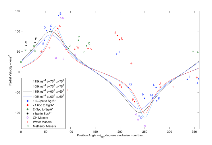
Figure 3.8: Plots of model radial velocities generated by varying the disk’s major axis angle to the sky’s horizon, $\phi$, and its inclination $\alpha$. As listed in the figure’s legend, rotational velocities of 105 and 115 km s^-1 were adopted as the upper and lower limits bracketing 110 km s^-1 see Table 3.4 . The effect of increasing the major axis orientation is to shift the curve horizontally to the left. Increasing the tilt angle increases the peak value of the radial velocity. The observed radial velocities of HCN(1-0)cores, Water, Methanol and OH masers are also plotted.

Sjouwerman and Pihlström (2008) identified OH masers near Cores B and N (cyan diamonds in Figs. 3.6, 3.7 and 3.8). The two masers in the NW lobe have highly positive radial velocities of +132km s^-1 which closely match the observed radial velocity of +139kms^-1 for Core B. The masers near Core N have highly negative radial velocities, –141 and –132km s^-1, compared with –64km s^-1 for Core N so appear unrelated to this core while associated with the two masers in the NW lobe. Two other OH masers with radial velocities of –104 and –117km s^-1 lie about a parsec outside Core O which has a radial velocity of +108 km s^-1 and could be in the same rotating streamer. Sjouwerman and Pihlström (2008) argue that the high velocities together with their symmetry of positive and negative values indicate that these masers are rotating in the CND structure. They contended that the source of excitation is collisions of CND cores and is not related to the supernova shell of SgrA East. Clumps of OH masers SE of the CND are indications of interaction between the expanding supernova shell and the +50km s^-1 molecular gas cloud.

3.8 HCN Core and Maser Radial Velocities

Fig. 3.8 shows model radial velocity curves based on combinations of $\phi$ = 60^∘ and 70^∘ clockwise from East and inclination angles, $\alpha$ = 60^∘ and 75^∘ to produce an envelope of curves that constrain the range of model radial velocity values. The core positions and observed radial velocities are superimposed for comparison with the model and an assessment made as to the likelihood of particular cores being located in the disk.

Both Table 3.5 and Fig. 3.7 indicate only five cores (F, G, X, Y and Z) lie outside a distance of 2pc from SgrA^∗ and eight cores (A, J, P, K, S, U, V and W) lie within 1.6pc from SgrA^∗. Six of the cores, (A, C, D, E, F and Z), are located in the NE section of the ring and nine cores, (J, K, L, M, N, O, P, Q and R) are in the SW section. This indicates that most of the detected HCN cores are located in the inner section of the CND(i.e. within 2pc of SgrA^∗).

Fig. 3.8 shows that the radial velocities of eight cores (B, H, S, T, U, V, X and Y) have large discrepancies, $>$35km s^-1, between observed and modelled radial velocities and do not appear to fit the model of a group of cores rotating about the galactic centre in circular orbits as part of the CND. All these cores, except U and V, lie between $\sim$ 1.6 and 3.5pc from SgrA^∗. Five cores (H, S, T, U and V) are located within a deprojected distance of $\sim$ 1.6pc of SgrA^∗ and may be influenced by the movement of ionised gas in the western arm of the mini-spiral which has positive radial velocities at these positions see Zhao et al. (2009) in contrast to the observed mainly negative velocities of these cores by Christopher et al. (2005). Cores X and Y are located in the linear filament that is located adjacent to the NW section of the CND (see Fig 1.3). Cores F and G are two outlier cores at deprojected distances more than 3pc east of the galactic centre and some 2pc inside the NE group of methanol masers reported by Sjouwerman and Pihlström (2008) as marking the shock front of the SgrA East supernova remnant (SNR) shell. Core B is located in the Northern Lobe close to the ring’s northern gap. The Northern Arm of the mini spiral is in the vicinity about 0.2pc to the west and 0.3pc to the South. Elements N1 and N2 of this feature have observed radial velocities of +78 and +100 km s^-1 respectively (see Table 3 of Zhao et al. (2009)) compared to the observed +139 km s^-1 for Core B. Assuming Core B and the two methanol masers are part of the CND requires that they be located in a CND streamer circulating at a much higher rotational velocity ($\sim$ 150 km s^-1) than the average 110 km s^-1.

3.9 Selection of HCN Cores for Analysis

The analysis using the LVG model relies on finding cores that have been observed in multiple transitions of HCN so that intensities for the three transitions can be matched to infer HCN column densities and hydrogen number densities. A literature review led to a choice of two groups of cores that had been observed in multiple transitions of HCN and that were physically and kinematically related. The first group of five cores were collated by Marr et al. (1993) who observed cores in H¹³CN(1-0) and HCO⁺(1-0) and convolved H¹²CN data (Guesten et al., 1987) and HCN(3-2) (Jackson et al., 1993) data with their observations. All the data was produced from unresolved images but had a consistent set of related intensities, spatial and kinematic properties which were modelled by Marr et al. (1993). This writer’s modelling is in effect a re-evaluation of the earlier analysis. The second group of seven cores were identified by the writer who selected data from three separate papers that described observations in three HCN transitions and HCO⁺(1-0). Core positions were established as described in Section 3.6 and kinematic properties established from data in the papers. Although four cores (A, B, C and E) from the first group are common to cores (D, W, Z and O) of the second group it has been decided to analyse these cores in their separate groups to provide a comparison between the results from unresolved data with results largely derived from resolved data.

The second group of cores were labelled independently by each author and located using a mixture of co-ordinates for the different HCN transitions (viz. B1950 for the (1-0) and (3-2) transitions and J2000 for the (4-3) transition). The cores observed in multiple transitions were identified by comparing locations using J2000 offsets from SgrA^∗ initially given in arcseconds (see Table 3.6) and subsequently converted to parsecs by dividing by 25.8 (based on a distance of 8 kpc to SgrA^∗).

The variety of telescopes used to observe the three transitions of HCN cores in the CND are listed in Table 3.9. The (1-0) and (4-3) observations are displayed with resolved, while the (3-2) observations are shown with unresolved maps.

[ht] HCN Observations HCN Paper Telescope Type Beam Size   ^a $\Delta$x $\Delta$y (1-0) Christopher et al. (2005) Ovens Valley Radio Obs Interferometer $5.1^{\prime\prime}$ $2.7^{\prime\prime}$ (3-2) Jackson et al. (1993) IRAM 30m Single Dish $12^{\prime\prime}$ $12^{\prime\prime}$ (4-3) Montero-Castaño et al. (2009) Sub mm Array Interferometer $4.6^{\prime\prime}$ $3.0^{\prime\prime}$

• Beam area is calculated as $\pi\Delta$x$\Delta$y/(4Ln2)

Identifying correspoding cores in the second group relies on the proximity of their spatial co-ordinates and their central spectral or radial velocities. Four of the seven objects, i.e. Cores D, M, W and Z have the strongest velocity space correlation and are undoubtedly cores observed in multiple HCN transitions. Cores I and O have anomalous central velocities for the (3-2) transition. These observations have been included on the basis that the spectra are from unresolved data, which can leave greater room for discrepancies given that they are visual estimates from the Jackson et al. (1993) figures. Core P has a lower central velocity in the HCN(4-3) transition, but has been included on the basis that it was one of the cores matched by Montero-Castaño et al. (2009) with the HCN(1-0) observations by Christopher et al. (2005). Fig. 7 in Montero-Castaño et al. (2009) shows the (1-0) and (4-3) spectra with double peaks and absorption occurs between the peaks in the (1-0) spectrum which combining the effects can explain the discrepancies (see Table3.9).

It should be noted that central velocities were only quantified by Christopher et al. (2005) in Table 2 of their paper for the (1-0) transition. Central velocities for the (3-2) and (4-3) transitions required visual estimates from the spectra provided in the relevant papers. Line widths were specified for the (1-0) and (4-3) transitions and had to be estimated for the (3-2) transition. The (3-2) transition spectral widths are large, due in some measure to the larger beam size.

[ht] Selected 2nd Core Group Spectral Properties HCN Core Central Velocity Spectral Width km s^-1 km s^-1 (1-0)^a (3-2)^b (4-3)^c (1-0) (3-2)^a (4-3)^d (1-0) (3-2)^d (4-3) D B A 101 100 110 45.5 80.0 38.5 I L AA -18 -50 -25 15.0 80.0 49.5 M H U -64 -50 -50 19.0 75.0 47.0 O G Q -108 -70 -90 36.5 90.0 51.0 P F N -73 -75 -40 28.2 75.0 97.0 W D F 56 45 50 27.9 45.0 40.0 Z C E 58 50 40 39.6 50.0 55.0

• core IDs from Christopher et al. (2005)

• core IDs assigned by this author by labelling spectra alphabetically from the top left in Fig. 1 of Jackson et al. (1993)

• core IDs from Montero-Castaño et al. (2009)

• Visual estimates

Table 3.9 and Fig. 3.9 show nine cores with the observations in three HCN transitions located in reasonable proximity of one another together with the offsets from SgrA^∗ in parsecs for the transition observations. Seven of these nine cores (D, I, M, O, P, W and Z) have their different transition observations within $\lesssim$ 7 arcseconds and generally within 2.6 arcsecs of their mean location and can be regarded as the same core especially given that the uncertainty of the positions of the HCN(3-2) cores are $\pm 0.25$pc or 6.5 arcsecs due to the beam size of the telescope. Cores H and L have the (1-0) and (4-3) transitions in close proximity but the (3-2) transition is too distant to be considered from the same core. For convenience the cores chosen for analysis shall be referred to by their Christopher et al. (2005) labels.

[!h]

Positions of Cores Identified in Multiple Transitions of HCN Core group Core ID for $\Delta$ RA $\Delta$ Dec Central Vel^a Mean Offset Position Core Posn rel to ID Transition Offset Offset VLSR $\Delta$RA $\Delta$Dec Mean Position pc pc km s^-1 pc pc pc pc D(1-0) 1.06 1.36 101 $-0.03$ $0.04$ D^b B(3-2) 1.15 1.56 100 1.09 1.32 $0.06$ $0.24$ A(4-3) 1.06 1.04 100 $0.08$ $-0.07$ H(1-0) 0.85 -0.03 -17 $0.05$ $-0.28$ H^f A(3-2) 0.75 0.39 0 0.80 0.25 $-0.05$ $0.14$ DD(4-3) 0.80 0.39 -5 $0.00$ $0.14$ I(1-0) 0.85 -0.38 -18 $0.02$ $0.0$ I L(3-2 0.77 -0.38 -50 0.83 -0.38 $-0.06$ $0.0$ AA(4-3) 0.88 -0.37 -25 $0.03$ $0.01$ L(1-0) 0.06 -1.29 -38 $-0.11$ $0.09$ L^f K(3-2) 0.39 -1.55 -50 0.17 -1.38 $0.22$ $-0.17$ W(4-3) 0.06 0.40 -50 $-0.11$ $0.08$ M(1-0) -0.12 -1.48 -64 $0.09$ $0.01$ M H(3-2) -0.38 1.55 -50 -0.21 -1.49 $-0.17$ $-0.06$ U(4-3) -0.13 -1.45 -50 $0.08$ $0.04$ O(1-0) -0.82 -1.24 -108 $0.01$ $0.07$ O^c G(3-2) -0.77 -1.55 -70 -0.81 -1.41 $0.04$ $-0.14$ Q(4-3) -0.83 -1.34 -90 $-0.02$ $0.06$ P(1-0) -0.82 -0.97 -73 $-0.01$ $0.07$ P F(3-2) -0.77 0.78 –75 -0.81 -0.86 $0.04$ $0.08$ N(4-3) -0.83 -0.83 -40 $-0.11$ $0.06$ W(1-0) -0.30 0.90 56 $0.03$ $0.02$ W^d D(3-2) -0.40 0.78 45 -0.33 0.88 $-0.07$ $-0.10$ F(4-3) -0.29 0.95 50 $0.04$ $0.07$ Z(1-0) -0.15 1.57 58 $-0.05$ $0.03$ Z^e C(3-2) -0.01 1.55 50 -0.10 1.54 $0.09$ $0.01$ E(4-3) -0.11 1.49 40 $-0.01$ $-0.05$

• Central velocity for (1-0) cores from Table 2 Christopher et al. (2005) velocities for (3-2) and (4-3) estimated visually by the thesis writer from spectra

• also associated with Core A Marr et al. (1993)

• also associated with Core E Marr et al. (1993)

• also associated with Core B Marr et al. (1993)

• also associated with Core C Marr et al. (1993)

• position of (3-2) transition too distant from (1-0) and (4-3) transitions not selected for group two

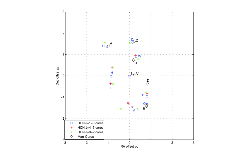
Figure 3.9: The figure shows positions of the two HCN core groups selected for LVG modelling. Locations of the first group are marked with black diamonds and have black labels useed by Marr et al. (1993). The location of the second core group transitions are marked with their respective symbols as shown in the legend and have blue labels used by Christopher et al. (2005). Offsets from SgrA^∗ are in parsecs based on the J2000 epoch.

3.10 Summary

A comparison of core radial velocities with model velocities corresponding to their deprojected positions in the CND showed that eighteen of the twenty-six cores have radial velocities consistent with being part of a disk rotating at $\sim$ 110 km s^-1. The spread of core radial velocities, when compared to the envelope of model velocity curves (see Fig. 3.8) is consistent with a disk composed of a series of rotating warped rings or streamers of gas (see Fig. 1.3 and Genzel (1989)). The methanol masers in the vicinity of Cores F, G and V have radial velocities consistent with the velocities of their neighbouring cores. Core B together with the OH masers in its vicinity form part of a higher rotational velocity streamer ($\sim$ 150 km s^-1) than the mean of 110 km s^-1

Fig. 3.7 showed the cores distributed in a circular pattern about SgrA^∗ with an inner cavity of about 1.6pc.

Two groups of cores have been selected for analysis based on having published data in three HCN transitions, the first group of five cores (A, B, C, D and E) have been taken from Marr et al. (1993), the second group of seven cores are Cores D, I, M, O, P, W and Z with their positions and central velocities listed in Table 3.9.

The next chapter covers the analysis of the core groups and the conclusions that can be drawn from the results.

Chapter 4 Analysis of HCN Cores

4.1 Introduction

In this chapter the Large Velocity Gradient model, described in Chapter 2, is used to simultaneously fit HCN and HCO⁺ line strengths in order to infer hydrogen number densities, optical depths and column densities of HCN and HCO⁺ in the CND cores.

Data for two separate HCN core groups selected from Chapter 3 are analysed:

1. Unresolved observations of the five cores (A to E) reported in Marr et al. (1993) that were observed in the (1-0) transitions of H¹²CN, H¹³CN, HCO⁺ and the (3-2) transition of HCN from Jackson et al. (1993). These results are given in Section 4.2.2

2. Seven cores (D, I, M, O, P, W and Z) identified as having observations in the (1-0), (3-2) and (4-3) transitions of HCN and the (1-0) transition of HCO⁺ reported in Christopher et al. (2005), Jackson et al. (1993) and Montero-Castaño et al. (2009). These results are given in Section 4.3.4.

Modelling was performed using the parameters reported in the papers and peak brightness temperature contours were plotted for values derived from the integrated intensity maps contained in the papers.

The modelling implies that the HCN(1-0), H¹³CN(1-0) and HCO⁺(1-0) lines are optically thin and weakly inverted. This is contrary to the findings of both Marr et al. (1993) and Christopher et al. (2005) who argued that the HCN (1-0) was optically thick. Reasons for the different outcomes are discussed in Section 4.4.

Results are presnted and comments made separately for each group before the Chapter closes with general discussion of both groups.

4.2 Group One

4.2.1 Input Data from Marr et al. (1993)

Peak brightness temperatures and FWHM velocities for Marr cores (A to E) identified by Marr et al. (1993) are reproduced here in Table 4.2.1. Core F was excluded from analysis by Marr et al. (1993) as its spectrum was considered to be affected by foreground absorption. The table summarises their observations of H¹³CN and HCO⁺ as well as data for H¹²CN from Guesten et al. (1987) and data for HCN (3-2) from Jackson et al. (1993) both remapped to scale with the Marr et al. (1993) H¹³CN and HCO⁺ data.

[!h]

Input Data from Marr et al. (1993)

	Central Vel	FWHM $\Delta$ V	Peak Brightness Temperature K
	km s-1	km s-1	H12CNa	HCO+	H13CN	HCN (3-2)b
Core A	$102$	50	3.6	3.8	0.8	4.4
Core B	$65$	60	4.8	3.4	1.3
Core C	$55$	60	2.9	3.0	1.3	2.5
Core D	$85$	75	3.0	$\leq 1.0$	0.7	2.1
Core E	$-96$	88	4.4	2.2	0.7	5.0

• original data from Guesten et al. (1987) convolved for Marr et al. (1993) beam

• original data from Jackson et al. (1993) convolved for Marr et al. (1993) beam

Molecular data for HCN and HCO⁺ were sourced from the Cologne Data Base for Molecular Spectroscopy. This data included excitation level information, Einstein A coefficients and collision rates for a range of kinetic temperatures and formed part of the input to the molecular rotation excitation model described in Chapter 2 that is used to analyse the observations.

150 K was chosen to be the fiducial value of the kinetic temperature for modelling as this was midway between 250 K, chosen by Marr et al. (1993) after considering a temperature range of (150 to 450 K) and 50 K, used by Christopher et al. (2005). The sensitivity to kinetic temperature was tested and the differences between 150 and 250 K can be seen by comparing Core A parameter values in Table 4.2.2. The excitation temperatures for all tracers increased at 250 K by between 7 and 18$\%$, optical depths decreased by 17$\%$ for H¹²CN and $7\%$ for H¹³CN, while they increased 0.3$\%$ for HCO⁺ and 3$\%$ for HCN (3-2). Peak brightness temperatures increased by 8$\%$ for H¹²CN but decreased by values ranging from 1 to 8$\%$ for the other three tracers.

4.2.2 Results

Each molecule was modelled by starting with local thermal equilibrium (LTE) by choosing a high atomic hydrogen density (10¹² cm^-3) and decreasing the density in steps of (logn_H = 0.1 to 10³ cm^-3) for each increasing step in molecular column density of (logN_col = 0.1) from 10¹² to 10¹⁸ cm^-2. Peak brightness values for the transitions were collected and plotted as contours to show how the specified brightness line (see Table 4.1) shifted with changing values of the two density parameters. The co-ordinates of the average of the intersection points of the brightness curves were taken as indicative values of a core’s hydrogen density and molecular column density per unit line width. The co-rdinate values from the core’s brightness plot were then applied to the plot of optical depths for the transitions and values taken where each optical depth curve intersected the co-ordinate point.

The modelling results for HCN column densities, hydrogen densities, excitation temperatures, optical depths and peak brightness temperatures for each transition are summarised in Table 4.2.2 and are shown in Figs. 4.1 to 4.6 which are contour plots of:

(a) The peak brightness temperature values for each of the molecules reported in Table 1 of Marr et al. (1993). The brightness values have an estimated accuracy of $\pm 0.2$ K and are derived from unresolved observations of the cores.

(b) Optical depths calculated by the model for the tracers, based on Eqn. 2.23.

The outputs from the model were plotted as contours on a log-log plot of HCN column density per unit line width (abscissa cm^-2/(km s^-1)) and atomic hydrogen number density (ordinate cm^-3).

The intersection of three contours can be regarded as a reliable indicator of the column densities of the molecular transitions and the hydrogen number density. Although the observations produced unresolved data the ratios of the brightness temperatures are assumed to be valid given that Marr et al. (1993) scaled data from other sources to match their H¹³CN(1-0) and HCO⁺(1-0) to allow comparison.

This approach is endorsed in section 4.1 of the Radex notes where the authors suggest the easiest way of solving the problem of unresolved images is to model intensity ratios and hope/argue that the beam dilution factor for the lines are comparable (van Langevelde and van de Tak, 2004). This approach has support from Marr et al. (1993) who stated in the results section of their paper that

• An overlay of HCO⁺ and H¹²CN data shows that HCO⁺ is distributed similarly to the HCN emission. Both are concentrated in the CND and are clumped at the same locations.

• Signals from H¹³CN are much weaker and closer to the noise level, with their brightest peaks located in the ring and with spectral centroids at the same velocities as the HCO⁺ and H¹²CN emission at the core positions. This means that the H¹³CN brightness data can be included in the analysis and provide reliable results when used with the brightness data from the other transitions.

The lesser abundant molecules were plotted over a lower range of column densities (see Table 4.2.2) and plotting consistency maintained by multiplying by the relevant abundance ratio to convert them to their H${12}$CN equivalent column densities. All tracers were plotted on the HCN column density scale divided by the relevant tracer’s line width.

[ht] Abundance Ratios of HCN to Other Modelled Molecules Molecule Normal Ratio^a Model Ratio Log Column Density Start Value Finish Value (cm^-2) (cm^-2) H¹²CN^b 1 1 12.0 18.0 H¹³CN 30 7.0 11.2 17.2 11.0^c 10.9 16.9 28^d 10.6 16.6 HCO⁺ $\sim$ 1 1.35^e 11.9 17.9 2.5^e 11.6 17.6

• as occurs in galactic clouds

• commonly referred to as HCN

• lower value in range Marr et al. (1993)

• higher value in range Marr et al. (1993)

• inverse of 0.74 quoted as average for CND value by Christopher et al. (2005)

• inverse of 0.4 quoted as the ratio corresponding to locations in the CND with peak HCN(1-0) emission Christopher et al. (2005)

Uncertainties arise with the [¹²C]/[¹³C] (Z ratios) as determined in Marr et al. (1993) from the rms noise in their data and standard error propagation through their equations relating $\tau$(H¹³CN), $\tau$(H¹²CN) and $\tau$(HCO⁺). Marr et al. (1993) noted that the lower boundary value of [HCN]/[H₂] = 6 $\times$ 10^-9 for their modelling occurred with values of Z = 4 to 7 which was subsequently superseded for a more reasonable value for [HCN]/[H₂] = 8 $\times$ 10^-8 and higher values for Z = 20. The effects of varying the value for Z are shown in Fig. 4.1 where brightness contours shift to the right for rising values of Z for both H¹³CN and HCO${+}$. The [¹²C]/[¹³C] abundance ratio is addressed more fully in Section 4.4.

The effect of varying the kinetic temperature from 150 to 250 K and Z values in the current model is shown for Core A in Figs. 4.1 and 4.2 and Table 4.2.2 with increases for H¹²CN of 12% in excitation temperature and 8% in brightness temperature and a decrease of 17% in optical depth occur. At Z = 7 the H¹³CN brightness temperature contour passes through the average of the intersection points and intersects the H¹²CN contour indicating that this is a more representative Z value for the prevailing conditions.

Table 4.2.2 lists the model parameters for Core A, where the H¹²CN and H¹³CN brightness contours are at their closest point of approach (logn_H =0.1). Ideally these curves should intersect and the fact that they do not can be attributed to the uncertainty in the value for Z:

• Fig. 4.1 Panel(a): for a kinetic temperature of T = 150 K this point occurs at about logn_h = 4.5 and logN_mol/dV = 13.7 where the excitation temperature for H¹²CN, T_ex = 6.5 K and optical depth, $\tau$ = 7.8. The corresponding values for H¹³CN are 3.8 K and 1.6 (see Table 4.2.2).

• Fig. 4.2 Panel(a): for 250 K this point occurs at about the same values of logn_h = 4.5 and logN_mol/dV = 13.7 where the excitation temperature for H¹²CN, T_ex is 7.2 K and optical depth, $\tau$ is 6.75. Values for H¹³CN are 4 K and 1.48 (see Table 4.2.2).

The modelling results for the points of closest approach show high H¹²CN optical depths ranging from about $\simeq$3 to 9. At these points the molecular hydrogen number density of 1.58$\times$ 10⁴cm^-3 is much lower than the density of $\simeq$ 10⁶cm^-3 inferred by Marr et al. (1993).

Table 4.2.2 includes Radex model results for the above points of closest approach for comparison with the Molex model. The agreement between the models is close for H¹²CN and acceptable for H¹³CN. For H¹²CN at 150 K the excitation temperature and optical depth from Radex are 0.5$\%$ higher while the brightness temperature is 0.6$\%$ lower than Molex. At 250 K the excitation temperature from Radex is 0.14$\%$ higher, the optical is depth 0.3$\%$ higher and the brightness temperature is 0.24$\%$ lower than Molex. The variations for H¹³CN at both kinetic temperatures are greater, with values up to 8$\%$ lower for Radex than Molex. The close agreement confirms that the Molex model is providing reliable results, and as Radex does not include dust extinction, it confirms that these dust parameters have a very small influence on the Molex results. This will be discussed further in Section 4.3.4 for the second core group where the dust parameters are varied in the Molex model to show minimal effect.

Panel (c) of Figs. 4.1 to 4.6 for the Marr cores shows contours of H¹²CN opacity calculated using brightness temperature values for H¹²CN and H¹³CN from the Molex model. The optical depths ranged from 0.9 to 1.3 when using a [C¹²]/[C¹³] ratio Z = 11, which is the minimum considered by Marr et al. (1993). Marr et al. (1993) cite an optical depth of 4, a kinetic temperature of 250 K and a molecular hydrogen density of $\approx$ 2.6$\times 10^{6}$ cm^-3 as more reasonable values from their modelling. For Core A, Eqn 4.6 produces $\tau$(H¹²CN) = 2.5 (see Table 4.2.2). An optical thickness of$\tau$(H¹²CN) = 4 would require a column density at least an order of magnitude greater. The reasons for the different results are again covered in Section 4.4.

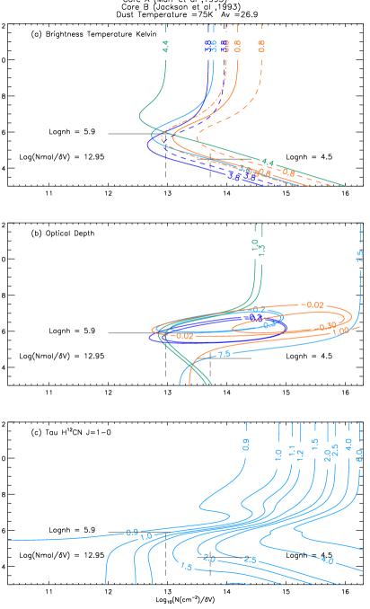
Figure 4.1: Panel (a) shows brightness temperature contours for H¹²CN, H¹³CN, HCO⁺ all (1-0) and HCN(3-2). H¹³CN with Z = 7 (chain dotted) and Z = 28 (dashed) and HCO⁺ with Z = 0.4 (dashed) contours are also plotted. The average intersection point of the species is logn_h = 5.9, log(N_mol/dV) = 12.95 with the closest point of approach of the contours at logn_h = 4.5, logN_Mol/dV) = 13.7. Panel (b) shows optical depth contours for the tracers. One abundance for both H¹³CN and HCO⁺ are plotted as indicated for clarity. H¹²CN, H¹³CN and HCO⁺ are optically thin with inverted transition populations, and HCN(3-2) is optically thin with $\tau$ $\sim$ 1.3. H¹²CN is optically thick with $\tau$ $\sim$ 7.5 at the closest point of approach of brightness contours. Panel (c) shows the optical depth contours of H¹²CN calculated using brightness temperatures for H¹²CN and H¹³CN from Molex and a [¹²C]/[¹³C] abundance ratio, Z = 11. $\tau^{12}$ = $\sim$ 1 at the average intersection point and $\sim$ 2.0 for the closest point of approach of the H¹²CN & H¹³CN brightness contours.

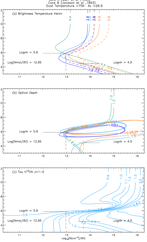
Figure 4.2: As for Fig. 4.1 with a raised kinetic temperature of 250 K. Panel (a) shows that the average intersection and closest approach points of the brightness temperature contours are unchanged from Fig. 4.1. Panel (b) shows optical depth contours the same as for the tracers in Fig. 4.1 Panel(c) shows the optical depth contours of H¹²CN from brightness temperatures for H¹²CN and H¹³CN calculated by Molex and a [¹²C]/[¹³C] abundance ratio Z = 11. Opacities are similar to Fig. 4.1

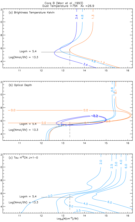
Figure 4.3: As in Fig. 4.1 but for Core B.

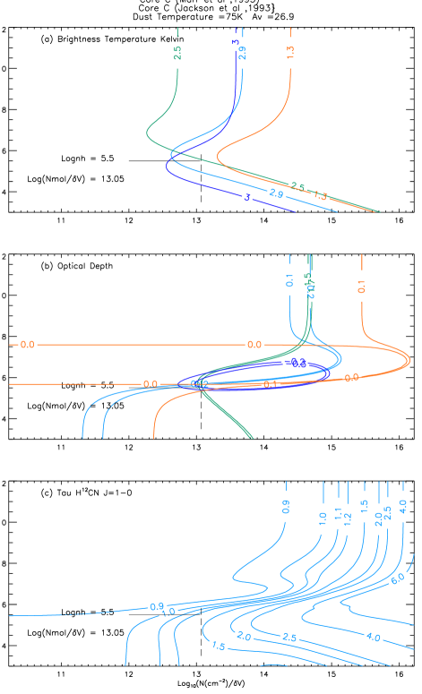
Figure 4.4: As in Fig. 4.1 but for Core C.

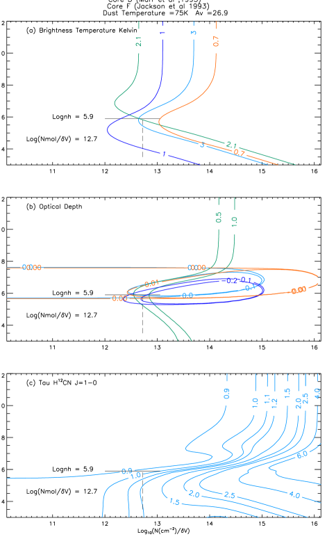
Figure 4.5: As in Fig. 4.1 but for Core D.

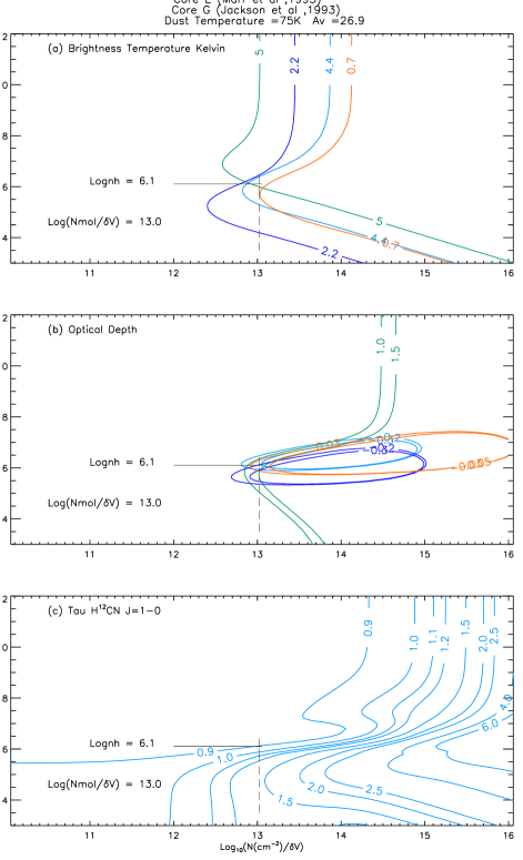
Figure 4.6: As in Fig. 4.1 but for Core E.

[ht]

Marr et al. (1993) Core Properties. Marr Core Gas Temp Average Log n(H₂) Excitation Temperature Tex Optical Depth $\tau$ Peak Brightness Temp T_b Tk Col Density H¹²CN H¹³CN HCO⁺ HCN H¹²CN H¹³CN HCO⁺ HCN H¹²CN H¹³CN HCO⁺ HCN per line 1-0 1-0 1-0 3-2 1-0 1-0 1-0 3-2 1-0 1-0 1-0 3-2 K cm^-2kms^-1 10${}^{6}\times$ cm^-3 K K K K K K K K A 150 12.95 0.397 -12.5 -16.3 -11.2 13.9 -0.195 -0.043 -0.214 0.777 3.42 0.85 3.49 4.51 A 250 12.95 0.397 -11.0 -13.4 -9.95 13.0 -0.228 -0.046 -0.208 0.803 3.69 0.84 3.09 4.17 % Difference 12.0 17.8 11.2 6.5 -16.9 -7.0 0.3 3.3 7.9 2.1 1.1 7.5 B 150 13.2 0.126 -27.6 12.6 -10.9 -0.161 0.150 -0.221 5.39 1.29 3.53 C 150 13.05 0.158 -16.1 9.21 -12.3 10.5 -0.145 0.215 -0.169 0.633 3.05 1.18 2.91 2.49 D 150 12.7 0.397 -22.6 19.6 -11.9 9.54 -0.105 0.049 -0.065 0.597 2.87 0.72 1.03 1.98 E 150 13.0 0.629 -11.1 5.23 -14.4 10.1 -0.215 0.217 -0.214 1.93 4.25 0.71 2.35 5.15

[ht] Marr et al. (1993) Core Parameters at Closest Point of Approach of H¹²CN and H¹³CN Brightness Contours

Core	Model	Tracer	Temp K	Hydrogena	LogNMol/dV	Column Densityb	Tex	$\tau$	Tb	$\beta$	x(u)	x(l)	Tb(H12CN)	$\tau$(H12CN)
				Density									/Tb(H13CN)
				(n(H2)$\times$104)		(NMol$\times 10^{15}$)
Ac	Molex	H12CN1-0	150	1.58	13.7	2.51	$6.50$	$7.84$	$3.52$	$0.185$	$0.49$	$0.31$	4.90	2.51
A	Radex	H12CN1-0	150	1.58		2.51	$6.53$	$7.88$	$3.50$		$0.49$	$0.31$
	%Difference						$0.46$	$0.51$	$-0.57$		$0.0$	$0.0$
A	Molex	H13CN1-0	150	1.58	13.7	0.228	$3.76$	$1.62$	$0.718$	$0.586$	$0.460$	$0.462$
A	Radex	H13CN1-0	150	1.58		0.228	$3.71$	$1.50$	$0.661$		$0.458$	$0.467$
	%Difference						$-1.33$	$-7.40$	$-7.93$		$-0.09$	$1.08$
Ad	Molex	H12CN1-0	250	1.58	13.7	2.51	$7.22$	$6.75$	$4.16$	$0.212$	$0.481$	$0.289$	4.76	2.587
A	Radex	H12CN1-0	250	1.58		2.51	$7.21$	$6.77$	$4.15$		$0.482$	$0.290$
	%Difference						$0.14$	$0.30$	$-0.24$		$0.21$	$0.35$
A	Molex	H13CN1-0	250	1.58	13.7	0.228	$4.01$	$1.48$	$0.87$	$0.610$	$0.469$	$0.439$
A	Radex	H13CN1-0	250	1.58		0.228	$3.96$	$1.37$	$0.81$		$0.467$	$0.439$
	%Difference						$-1.25$	$-7.43$	$-6.90$		$-0.42$	$0.0$
Be	Molex	H12CN1-0	150	1.58	13.9	4.77	$7.9$	$9.84$	$4.83$				5.43
B	Molex	H13CN1-0	150	1.58		0.43	$3.9$	$2.04$	$0.89$
Cf	Molex	H12CN1-0	150	na	na	na	${\mathrm{na}}$	${\mathrm{na}}$	${\mathrm{na}}$				na
C	Molex	H13CN1-0	150	na	na	na	${\mathrm{na}}$	${\mathrm{na}}$	${\mathrm{na}}$				na
Dg	Molex	H12CN1-0	150	1.58	13.7	3.76	$6.68$	$8.05$	$3.64$				5.87
D	Molex	H13CN1-0	150	1.58		0.34	$3.69$	$1.39$	$0.62$
Eh	Molex	H12CN1-0	150	0.50	13.3	1.76	$7.69$	$2.27$	$4.15$				5.85
E	Molex	H12CN1-0	150	0.50		0.16	$5.23$	$0.38$	$0.71$

• molecular hydrogen density, n${}_{H_{2}}$, calculated as 0.5 atomic hydrogen density, n(H)

• N${}_{\mathrm{molH}}^{13}$CN is derived by dividing Nmol H¹²CN by 11

• see Fig. 4.1

• see . 4.2

• see Fig. 4.3

• there is no point of closest approach see Fig. 4.4

• see Fig. 4.5

• contours intersect see Fig. 4.6

Table 4.2.2 summarises the results for the five HCN cores (A to E) reported in Marr et al. (1993). The average column density per line width and atomic hydrogen number density for each core were obtained by averaging the values of the intersection points of species pairs H¹²CN(1-0)/HCN(3-2), HCO⁺(1-0)/H¹²CN(1-0) and H¹³CN(1-0)/HCN(3-2) to provide brightness temperature values that match the plotted contour values.

It is notable that the H¹²CN and H¹³CN brightness contours only intersect for Core E (Fig. 4.6) and do not closely approach each other in the plot for Core C (Fig. 4.4). The three remaining cores, A, B and D, have close approach points listed in Table 4.2.2.

4.2.3 Comments

Marr et al. (1993) used a statistical equilibrium excitation model for HCN and set boundary values for kinetic temperature (150 to 450 K), dust temperature of 75 K, optical depth (1 to 12) and [HCN]/[H₂] ratios (6$\times$ 10${-9}$ to 3$\times$10_-6. The [¹²C]/[¹³C] ratio (Z) was assumed to vary between 10 and 40 while noting that previous estimates varied from 11 (in SgrB₂ (Mangum et al., 1988)) to 28 ( in the galactic centre (Wannier, 1989)).

Fig. 4.1 Panel (a) showed brightness contours for Core A with alternative abundance ratios Z = 7 and Z = 28 for [H¹²CN]/[H¹³CN] and Z = 0.4 for [HCO⁺]/[HCN] as dashed contours. The alternative ratios of Z = 28 and Z = 0.4 do not provide a definitive intersection of the contours with the H¹²CN contour. The contours for Z = 7 and Z = 0.4 do intersect the H¹²CN contour but at a lower hydrogen density value than for Z = 11 and Z = 0.74 which led to the adoption of Z = 11 and Z = 0.74 for the other core plots. It should also be noted that the intersection area for all tracers is not representative of the closest approach ($\Delta$logn_H = 0.1) of the H¹²CN and H¹³CN contours, which are closest to each other over a span of log column density per line width ($\delta$V) values from 13.6 to 14.

The effect of changing the abundance ratio is shown in Fig. 4.1 Panel(a) where the relevant brightness contours shift to the left as the ratio decreases. This is especially noticeable for the [C¹²]/[C¹³] = 7 curve where the contour falls within the intersection points of the other three species. Similarly, a reduction in the brightness temperature shifts the contour to the left.

The excitation temperatures of all species and transitions are different from each other. Stimulated emission is occurring in the H¹²CN, H¹³CN and HCO⁺ species; this was not considered by Marr et al. (1993) where maser emission was excluded from their analysis. The current results show that inverted transition levels are occurring and are optically thin not thick as suggested by Marr et al. (1993).

4.3 Group Two

Sections 4.3.1 to 4.3.3 describe the core input data for the HCN(1-0), (3-2) and (4-3) transitions and the HCO${+}$(1-0) transition.

4.3.1 HCN(1-0) and HCO⁺(1-0) Input

The integrated intensity of each of the HCN(1-0) cores was obtained from Fig. 13 of Christopher et al. (2005) by counting the contour levels from the lowest level to the contour closest to the core to obtain an estimated peak integrated intensity in Jy beam^-1 km s^-1. The beam quoted in the paper was converted to steradians and the FWHM spectral width for each core in km s^-1 was obtained from Table 2 of their paper. The integrated intensity was divided by the beam’s area and the line width to produce a peak intensity at line centre I_ν(0). Peak radiation temperatures at line centre were then derived using the following Rayleigh-Jeans relationship:

$$\mathrm{T_{b}}=\mathrm{I}_{\nu}(0)\lambda^{2}\times 10^{-23}/2\mathrm{k}\,.$$ (4.1)

HCO⁺(1-0) intensities were obtained from the integrated intensities in Fig. 4 of Christopher et al. (2005) and processed in the same manner as for the HCN (1-0) data described above.

Table 4.1 summarises the input for both tracers. Core data, central velocities and line widths are assumed to be the same as for the HCN(1-0) data.

Table 4.1: Input Data from Christopher et al. (2005)

HCN (1-0)	Diameter	Area	Central Vel	Line Width	Contour Value	Integ Intensity	Peak Tb
	FWHM pc	arsecs2	km s-1	km s-1	6.675$\times$Jy beam-1km s-1	Jy beam-1km s-1	K
Core D	0.43	96.5	101	45.5	4.5	30.4	7.6
Core I	0.26	35.3	-18	15	1.5	10.1	7.6
Core M	0.26	35.3	-64	19	3.5	23.7	14.1
Core O	0.33	56.9	-108	36.5	6.0	40.6	12.6
Core P	0.21	23.0	-73	28.2	4.5	30.4	12.2
Core W	0.22	25.3	56	27.9	2.5	16.9	6.8
Core Z	0.24	25.3	58	39.6	2.5	16.9	4.8
HCO+ (1-0)
Core D					2.0	13.53	3.3
Core I					0.8	5.412	4.0
Core M					1.0	6.765	4.0
Core O					1.5	10.15	3.1
Core P					2.0	13.53	5.4
Core W					2.0	13.53	5.4
Core Z					1.5	10.15	2.9

4.3.2 HCN(3-2)

The appropriate HCN(3-2) core to match the (1-0) core was determined in Chapter 3 by comparing x and y offsets from SgrA^∗ of the (1-0) and (3-2) cores and selecting the closest match (see Table 3.9). Peak brightness temperatures for the HCN (3-2) transition were obtained from visual estimates of the spectral values plotted in Fig. 1 of Jackson et al. (1993), where the emission was plotted as Tb versus $\delta$V km s^-1. Line widths were obtained by measuring the spectral width at the half maximum T_b level.

A core diameter of 0.25pc (6.45”), based on the average core diameter in Table 2 of Christopher et al. (2005), was used to calculate a dilution factor of $32.7/163=0.2$. The peak brightness temperature interpreted from the spectra were then divided by 0.2 to produce the “resolved” brightness temperatures used to plot the HCN(3-2) contours. Resolved (3-2) brightness temperatures are required to produce plots that are consistent with the resolved (1-0) and (4-3) data, where the cores fill the telescope’s beam whereas the (3-2) data only fills 0.2 of the beam (see Table 3.9). Additional brightness temperatures for Core D of 6.7 K and 11.4 K for Core O are based on the dilution factors for diameters of these two cores listed in Table 2 of Christopher et al. (2005).

[ht] Input Data from Jackson et al. (1993)

Jackson et al. (1993)	Christopher et al. (2005)	Central Vel	Line Width	Observed	Resolveda
	Equivalent Core	km s-1	km s-1	Peak Tb K	Peak Tb K
Core B	Core Db	100	80	5	25
Core L	Core I	-50	80	3	15
Core H	Core M	-50	75	6	30
Core G	Core Oc	-25	90	5	25
Core F	Core P	-40	75	4.75	23.7
Core D	Core W	25	45	3.60	18
Core C	Core Z	50	50	2.60	13

• based on a dilution factor of 0.2

• based on Core D diameter of 0.43pc dilution factor of 0.75 the resolved Tb is 6.7 K

• based on Core O diameter of 0.33pc dilution factor of 0.44 the resolved Tb is 11.4 K

4.3.3 HCN (4-3)

The appropriate cores corresponding to the (1-0) core were selected by comparing co-ordinates, from (Montero-Castaño private communication) with the HCN (1-0) core co-ordinates (see Table 3.9). HCN (4-3) peak brightness temperatures were obtained from Fig. 7 of Montero-Castaño et al. (2009) using the Rayleigh-Jeans relationship (see Eqn 4.1 with the line centre intensity,I_ν(0) obtained by dividing the integrated intensity expressed as Jy beam^-1 by the beam area in steradians.

The core FWHM velocities in Table 4.3.3 were obtained from Table 1 of Montero-Castaño et al. (2009).

[ht] Input Data from Montero-Castaño et al. (2009) Montero-Castaño et al. (2009) Christopher et al. (2005) Core Radius^a Core Area Central Vel^b Line Width^a Int Emission^b Peak Tb^c pc arcsecs² km s^-1 km s^-1 Jy beam^-1 K Core A Core D 0.139 40.04 110 38.5 6.5 4.6 Core AA Core I 0.145 43.9 -25 49.5 4.0 2.8 Core U Core M 0.110 25.3 -50 47.0 16 11.3 Core Q Core O 0.161 54.1 -90 51.0 14.2 10.0 Core N Core P 0.253 134 -40 97.0 11.0 7.8 Core F Core W 0.092 17.7 50 40.0 6.5 4.6 Core E Core Z 0.098 20.1 40 55.0 8.3 5.9

• from Montero-Castaño et al. (2009) Table 1

• estimated from spectra in Montero-Castaño et al. (2009) Fig. 7 beam 4”.6 $\times$ 3”.0

• calculated from estimated integrated emission using Eqn 4.1

A kinetic gas temperature of 150 K was again adopted for all seven cores. Additional modelling of Cores D and M was performed at a kinetic temperature of 50 K to compare the effects on the hydrogen density value by reducing the kinetic temperature to the value used by Christopher et al. (2005).

Model output for the seven cores was plotted as contours of brightness temperatures (as listed in Tables 4.1 to 4.3.3) in Figs. 4.7 to 4.15.

Christopher et al. (2005) quote a variation in dust temperatures from 20 to 80 K and adopts T = 50 K and an Av = 30 in their calculations compared with T = 75 K and Av = 26.9, calculated using Eqn 2.53, and adopted for the current modelling. 75 K was chosen as a mid value between dust temperatures of 50 to 90 K quoted in Table 1 of Genzel (1989). Genzel mentions sub-millimetre dust emission detected by Mezger et al. (1989) which is interpreted as cold dust with a temperature of 10 to 20 K. Mezger et al. (1989) quote Wade et al. (1987) finding a uniform extinction of $\sim$ 27 towards the central 0${}^{{}^{\prime}}$.5 of the galactic centre.

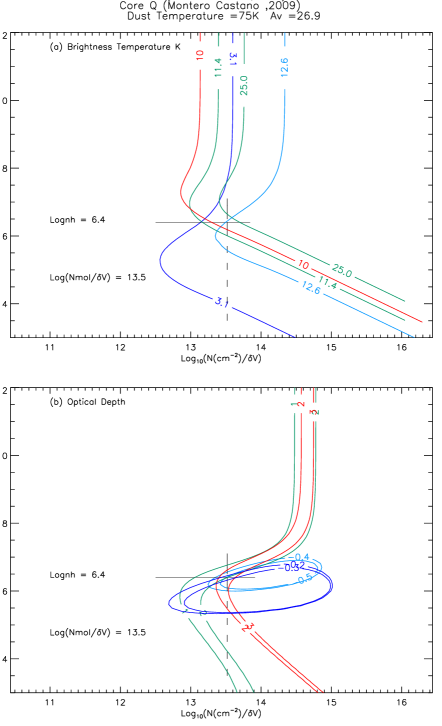
Figure 4.12: As for Fig. 4.7 but for Core O.

Core O is modelled with and without dust to show that Molex was insensitive to dust emission at the HCN transition frequencies being analysed. Table 4.2 confirms that these are very small differences, generally less than 0.1$\%$, between model outputs for the two cases, this is because the radiation effects are highly diminished at wavelengths $>$ 1000$\mu$m. For example the optical depth of the dust at 846 $\mu$m) (the wavelength of HCN(4-3)) is 4.76 $\times$ 10^-4 produces 0.03 K (T_b (dust) = $\tau_{\mathrm{dust}}\times$ T(dust)) as the brightness temperature for dust with a kinetic temperature of 75 K. Comparison of Figs. 4.12 and 4.13 shows that the differences are undetectable in the plots of brightness temperatures and optical depths.

4.3.4 Results

The results for these seven cores were obtained by averaging the values of intersection points of pairs of species in Figs. 4.7 to 4.16 and are summarised in Table 4.3.5. The molecular hydrogen densities range from n_H2 = 0.79 (Core I) to 1.58 (Core M) $\times 10^{6}$cm^-3 for a kinetic temperature of T = 150 K; these are less than a quarter to a half of the values for the optically thin scenario of Christopher et al. (2005) for the HCN(1-0) transition. Modelling Cores D and M with a kinetic temperature of T - 50 K produces a value of n_H2 = 3.97$\times 10^{6}$cm^-3 see Table 4.3.5).

Table 4.3.5 summarises the results for optical depth for the seven cores where the HCN(1-0) and HCO⁺(1-0) transitions indicate the presence of stimulated emission with negative excitation temperatures and opacities. The opacities range from 1.11 to 1.96 for HCN(3-2) and 1.0 to 2.57 for HCN(4-3).

The HCN column and atomic hydrogen number density values were obtained from averaging the values at the species intersection points for the brightness temperatures of HCN(1-0) with the other transitions. For example in Fig. 4.15 describing Core W the intersection of HCN(1-0), HCN(4-3) and HCO⁺(1-0) was the lower point at logN_col/$\delta$V = 13.2 and logn_h = 6.1, with the intersection of HCN(1-0) and (3-2) the upper point at logN_col/$\delta$V = 13.4 and logn_H = 6.6. The average values of log Column density/$\delta$V = 13.3 and logn_H = 6.25 were the result of averaging the values of these two intersection points. It should be noted that the lower limit curve of 12.6 K for the (3-2) transition provides a tighter intersection envelope and slightly lower values for both HCN column and hydrogen number densities.

4.3.5 Comments

The seven HCN cores provide a good representative sample of CND conditions as they are spread throughout the ring. Core D is in the Northeast, Core I is in the East, Core M is in the South, Cores O & P are in the Southwest and Cores W & Z are in the North (see Fig. 3.9).

Using the 0.2 dilution factor for the HCN(3-2) transition results in peak brightness temperature contours that have a spread of intersection points with the other HCN and HCO⁺ contours; these lead to upper and lower limits for the both hydrogen number and HCN column densities.

The accuracy of the HCN(3-2) peak brightness temperatures is stated by Jackson et al. (1993) to be $\pm 30\%$ due to the relatively large beam size of about 12”, compared to the average core size of 6.5”, this also contributes to the large line widths for this transition compared to the other transitions of HCN and HCO⁺ for this group of cores (see column 4 of Table 4.3.2). The effect of the large error spread can be seen in the plot of brightness temperatures for Core W in Fig. 4.15, where the lower brightness temperature contour more closely fits the contours of the other transitions than the average HCN(3-2) brightness temperature.

For Core D Fig. 4.7 (a) shows contours for three values of the $[\mathrm{HCO^{+}}]/[\mathrm{HCN}]$ abundance ratios, Z = 0.4, 0.74 and 1.2, (reported by Christopher et al. (2005) as occurring in the CND). Lowering the abundance ratio reduces the column density per line width value. Again in modelling the second group of HCN cores the mean HCO⁺ abundance value of 0.74 was used in all plots, in contrast to the value of 0.4 used by Christopher et al. (2005) to outline the regions of relatively high HCN emission and low HCO⁺ emission.

The molecular hydrogen number density for the seven HCN cores varies from 0.95 (Core I) to 1.9 (Core M) $\times 10^{6}$cm^-3, which is an order of magnitude lower than the value n${}_{H_{2}}$ = 10⁷cm^-3 reported by Christopher et al. (2005) for HCN(1-0) gas with $\large{\tau}$ = 4 . The model results support an optically thin model as they are even lower than the results for the optically thin gas scenario reported in Christopher et al. (2005) (see Table 4.3.5).

Table 4.3.5 provides a comparison between the three core density scenarios (virial, optically thin $\tau$ _HCN(1-0) $\leq$ 1 and optically thick $\tau$ _HCN(1-0) = 4) discussed in Christopher et al. (2005) and those obtained from modelling the HCN cores identified in this thesis.

Cores D and M were also modelled using a kinetic temperature of 50 K, which produced molecular hydrogen densities for both of n${}_{\mathrm{H}_{2}}$ = 3.97$\times 10^{6}$ cm^-3, which agrees closely with the Christopher et al. (2005) values under optically thin conditions. The brightness temperature value of the HCN(3-2) transition contours in Cores D and O was varied to account for the different dilution factor when using the core sizes listed in Table 4.3.5 instead of the average 0.25 pc size adopted for calculating the 0.2 dilution factor in Table 4.3.2. Figs. 4.7 and 4.12 show that the HCN(3-2) brightness contour shifts to the left as the brightness temperature decreases, so that it forms a tighter intersection area with the other HCN transitions. The resulting molecular hydrogen number density and HCN column density per line width are slightly lower than the tabulated values in Table 4.3.5 e.g. log(n_H) = 6.3 and log(N_mol/dV) = 13.2 compared with log(n_H) = 6.4 and log(N_mol/dV) = 13.5 for Core O.

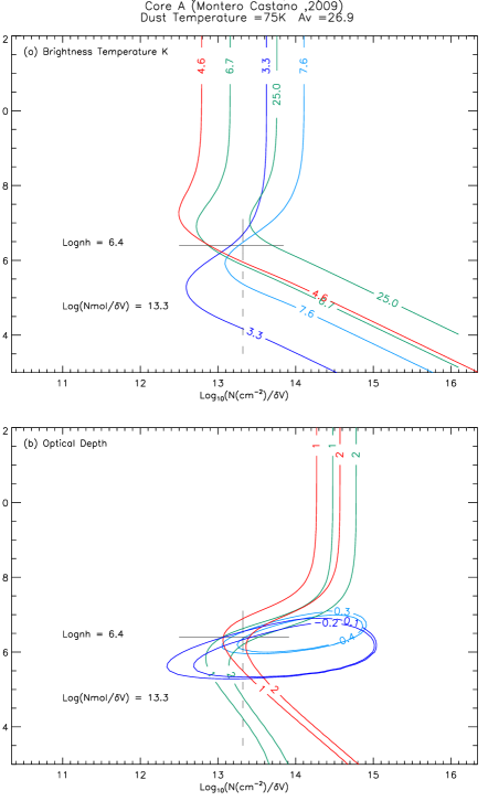
Figure 4.7: Core D with kinetic temperature of 150 K. Panel (a) shows brightness temperature contours for HCN (1-0), (3-2), (4-3) and HCO⁺ (1-0). The average intersection point of the species is log(n_H) = 6.4, log(NMol/dV) = 13.3. Panel (b) shows the optical depth contours for the tracers which are optically thin and shows inverted populations of HCN(1-0) and HCO⁺(1-0).

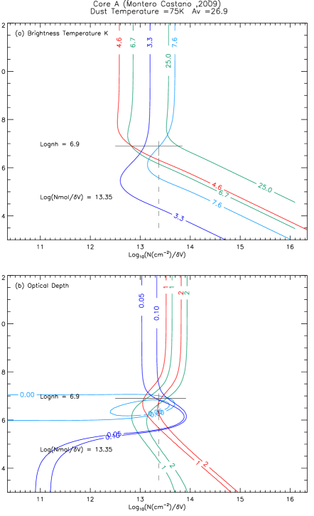
Figure 4.8: As for Fig. 4.7 but with the kinetic temperature of I = 50 K used by Christopher et al. (2005).

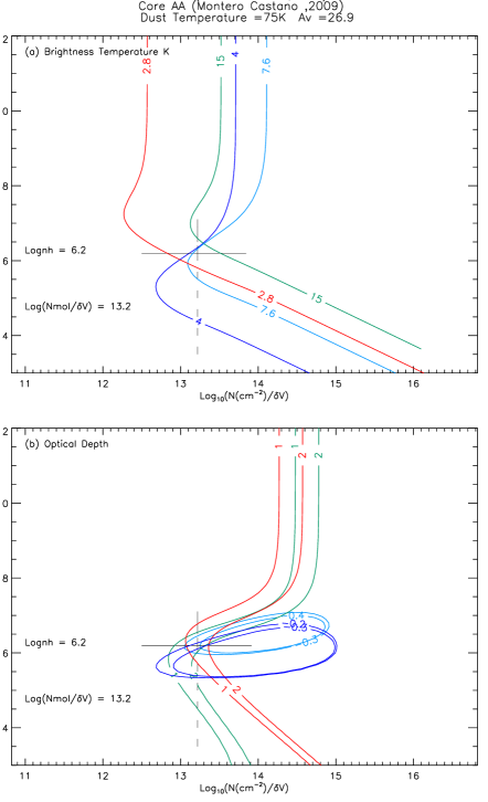
Figure 4.9: As for Fig. 4.7 but for Core I.

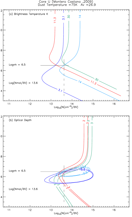
Figure 4.10: As for Fig. 4.7 but for Core M at kinetic temperature of T = 150 K.

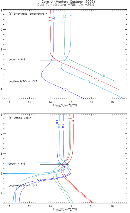
Figure 4.11: As for Fig. 4.10 but with a kinetic temperature of T = 50 K.

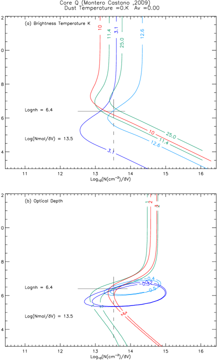
Figure 4.13: As for Fig. 4.12 but with no dust.

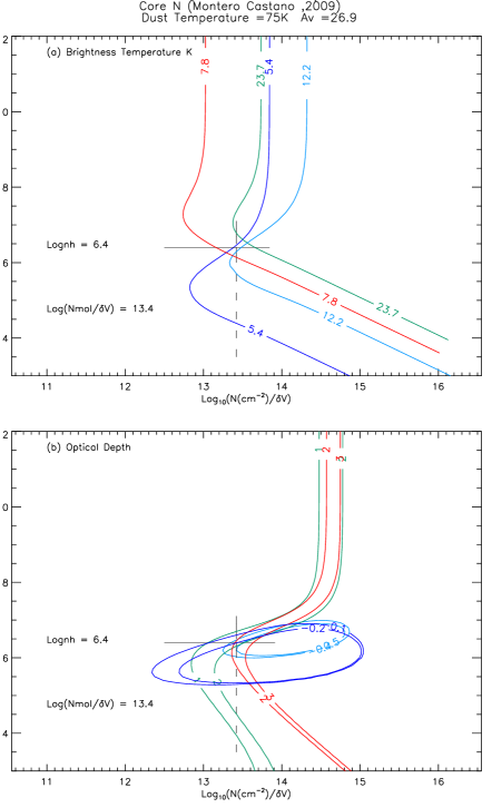
Figure 4.14: As for Fig. 4.7 but for Core P.

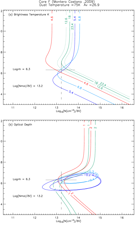
Figure 4.15: As for Fig. 4.7 but for Core W.

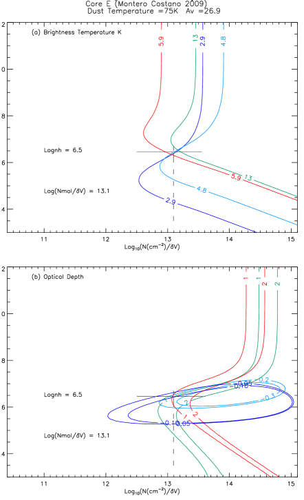
Figure 4.16: As for Fig. 4.7 but for Core Z.

[ht]

HCN Core Properties. Group 2 Cores Kinetic Average Log n(H₂) Tex K Optical Depth $\tau$ Peak Brightness Temp Tb K Temp Col Density HCN HCN HCN HCO⁺ HCN HCN HCN HCO⁺ HCN HCN HCN HCO⁺ per line 1-0 (3-2) (4-3) (1-0) (1-0) (3-2) (4-3) (1-0) (1-0) (3-2) (4-3) (1-0) (K) (cm^-2/km s^-1) (10${}^{6}\times$cm^-3) (K) (K) (K) (K) (K) K (K) (K) D $150$ $13.3$ $1.26$ $-21.9$ $44.0$ $13.1$ $-23.0$ -0.30 1.11 1.06 -0.15 8.9 25.30 4.14 4.18 D $50$ $13.4$ $3.97$ $-353.0$ $38.7$ $13.2$ $749.0$ -0.04 1.25 1.45 0.01 8.45 23.2 4.9 4.49 I $150$ $13.2$ $0.79$ $-15.8$ $28.6$ $11.8$ $-29.20$ -0.33 1.29 1.66 -0.21 7.43 16.3 4.14 3.51 M $150$ $13.6$ $1.58$ $-21.7$ $45.7$ $21.8$ $-28.7$ -0.52 1.94 2.57 -0.08 17.4 32.8 12.3 2.78 M $50$ $13.7$ $3.97$ $336.0$ $38.1$ $18.9$ $88.5$ 0.04 2.70 3.50 0.07 14.2 29.7 11.3 5.67 O $150$ $13.5$ $1.26$ $-18.5$ $36.1$ $18.2$ $-28.7$ -0.52 1.96 2.30 -0.09 15.0 25.8 9.8 2.89 P $150$ $13.5$ $1.0$ $-18.6$ $35.8$ $16.8$ $-34.2$ -0.53 1.93 2.23 -0.27 15.4 25.3 8.9 11.6 W $150$ $13.2$ $1.0$ $-17.2$ $19.4$ $14.2$ $-13.4$ -0.24 1.80 0.95 -0.29 6.14 11.0 4.46 5.55 Z $150$ $13.1$ $1.58$ $-14.8$ $31.0$ $17.6$ $-21.9$ -0.25 0.9 1.0 -0.1 5.1 14.6 6.5 3.1

Table 4.2: Effects of Variations in Dust Extinction for Core O.

Tracer	lognH	logNmol	Td	Av	Tex	Optical	Tb	$\beta$	Intensity	Int Intensity	Upper	Lower
	cm-3	(cm-2km s-1)	(K)		(K)	Depth	(K)		(erg cm-2 s-1 sr-1)	(K km s-1)	level	level
HCN (1-0)	$6.4$	$13.5$	0	$0.0$	$-20.1$	$-0.44$	$13.0$	$1.19$	3.15E-14	$504.0$	$0.193$	$0.052$
	$6.4$	$13.5$	75	$26.9$	$-20.1$	$-0.44$	$13.0$	$1.19$	3.15E-14	$504.0$	$0.193$	$0.052$
% Difference					$0.03$	$-0.09$	$-0.07$	$-0.02$	-0.07	$-0.07$	$-0.06$	$-0.06$
HCO+ (1-0)	$6.4$	$13.5$	0	$0.0$	$-23.9$	$-0.22$	$6.62$	$1.09$	1.62E-14	$256.0$	$0.101$	$0.028$
	$6.4$	$13.5$	75	$26.9$	$-23.9$	$-0.22$	$6.62$	$1.09$	1.62E-14	$256.0$	$0.101$	$0.028$
% Difference				$0.04$	$-0.08$	$-0.04$	$0$	$-0.04$	-0.04	$-0.04$	$-0.03$
HCN (3-2)	$6.4$	$13.5$	0	$0.0$	$29.4$	$2.06$	$20.4$	$0.518$	4.42E-13	$1940.0$	$0.241$	$0.266$
	$6.4$	$13.5$	75	$26.9$	$29.4$	$2.06$	$20.3$	$0.518$	4.42E-13	$1940.0$	$0.241$	$0.266$
% Difference				$0.0$	$-0.07$	$0.09$	$0.01$	$-0.09$	-0.09	$-0.06$	$-0.06$
HCN (4-3)	$6.4$	$13.5$	0	$0.0$	$22.7$	$2.36$	$13.7$	$0.48$	5.31E-13	$743.0$	$0.146$	$0.241$
	$6.4$	$13.5$	75	$26.9$	$22.7$	$2.36$	$13.7$	$0.48$	5.31E-13	$743.0$	$0.146$	$0.241$
% Difference				$0.10$	$-0.13$	$-0.09$	$0.08$	$-0.08$	-0.08	$0.03$	$-0.05$

Table 4.3: Radex Calculations vs Molex for Core O.

Model	Tracer	Frequency	dV	lognH	n${}_{H_{2}}$	logNMol	NMol	Tex	Optical	Tb
									Depth
		(GHz)	(km s-1)		($\times 10^{6}$ cm-3)		($\times 10^{15}$ cm-2)	(K)	($\tau$)	(K)
Molex	HCN (1-0)	88.6316	$36.5$	$6.5$	1.9	15.2	1.433	$-21.60$	$-0.45$	$14.2$
Radex				$6.5$	1.9	15.2	1.433	$-20.90$	$-0.43$	$13.1$
% Difference								$-3.2$	$-4.2$	$-8.0$
Molex	HCO+ (1-0)	89.1885	$36.5$	$6.7$	3.0	14.9	0.794	$-54.4$	$-0.08$	$4.6$
Radex				$6.7$	3.0	14.9	0.794	$-60.3$	$-0.07$	$4.5$
% Difference								$-10.8$	$10.5$	$-2.2$
Molex	HCN (3-2)	256.8864	$90$	$6.7$	3.0	15.5	2.818	$42.8$	$1.11$	$25.4$
Radex				$6.7$	3.0	15.5	2.818	$43.54$	$1.12$	$25.2$
% Difference								$1.7$	$0.9$	$-0.6$
Molex	HCN (4-3)	354.5055	$51$	$6.5$	1.9	15.1	1.258	$23.8$	$1.82$	$13.7$
Radex				$6.5$	1.9	15.1	1.258	$23.7$	$1.83$	$13.6$
% Difference								$-0.4$	$0.6$	$-1.0$

[!h]

HCN Cores Published Vs Modelled Properties.

Christopher et al. (2005)	Deproj Dist	Size FWHM	Christopher et al. (2005) H2 Density Scenarios			Modelleda
ID			Virial	Opt thick	Opt thin	H2 Density	$\tau$ HCN(1-0)
				$\tau$ =4
	(pc)	(pc)	($\times$106cm-3)	($\times$106cm-3)	($\times$106cm-3)	($\times$106cm-3)
Db	1.86	0.43	32.29	49.41	3.97	1.51	-0.30
I	1.87	0.26	9.68	27.06	2.06	0.95	-0.33
Mc	1.75	0.26	14.78	33.43	3.56	1.90	-0.52
O	1.60	0.33	35.04	51.48	7.36	1.51	-0.52
P	1.39	0.21	50.82	62.00	7.06	1.20	-0.24
W	1.47	0.22	45.28	58.32	5.44	1.20	-0.24
Z	2.08	0.24	78.22	76.91	2.37	1.58	-0.25

• Values for hydrogen density and HCN(1-0) optical depth based on a kinetic temperature of 150 K

• Core D modelled hydrogen density for Tk=50 K is 3.97$\times 10^{6}$cm^-3 which agrees with Christopher et al. (2005)

• Core M modelled hydrogen density for Tk=50 K is 3.97$\times 10^{6}$cm^-3 compared with 3.56$\times 10^{6}$cm^-3 in Christopher et al. (2005)
  

4.4 Discussion

The current modelling results have shown that molecular hydrogen densities are about 10⁶cm^-3 and optical depths for the HCN(1-0) transition are $\ll$ 1. The reason for this difference from previous results is discussed in this section which highlights the modelling outcomes of both core groups. The fact that the argument of Marr et al. (1993) for equal excitation temperatures for the HCN isotopologs does not hold true for optically thin, inverted transitions as occur for HCN(1-0) and HCO⁺(1-0) transitions helps explain the different results.

The accuracy of the modelling was checked by comparing output parameter values with specific values for these parameters generated by Radex. Tables 4.2.2 and 4.3 show the Radex results for Core A in the first group and Core O in the second group confirm that the results from LVG analysis for these cores are reasonable and that the LVG modelling give reliable results.

Marr et al. (1993) used an excitation model which predicted HCN brightness temperatures, opacities and excitation temperatures for the first 20 excitation levels. The assumption was made that based on previous estimates Z varied from 10 to 40 and core sizes that were inferred from the beam filling factor and beam size varied from 0.05 to 0.12pc.

Uncertainty about the value of Z arises from the fact that Marr et al. (1993) found the value of Z from modelling was between 4 and 7 to satisfy their low boundary condition for the [HCN]/[H₂] abundance of 6$\times$10^-9 at a kinetic temperature of 150 K and $\tau_{\mathrm{HCN}(1-0)}$ = 1. These Z values agree with those from current modelling of $\sim$ 3 to 6 from the ratios of core T_bH¹²CN to T_bH¹³CN (using Eqn. 4.3). Marr et al. (1993) then reasoned that 250 K was a more reasonable kinetic temperature based on other CND studies and assuming a Z value of 20 produced a hydrogen density of n${}_{H_{2}}$ = 2$\times$10⁶cm^-3 best fitted their observed brightness temperatures.

The current modelling for a kinetic temperature of 250 K found the hydrogen density unchanged at 0.4$\times$10⁶cm^-3 (see Table 4.2.2). Marr et al. (1993) also concluded that with their more reasonable parameters the [HCN]/[H₂] abundance was 8$\times$10^-8 an order of magnitude greater than the typical interstellar abundance of 10^-9 which was used by Christopher et al. (2005).

The underlying assumption of Marr et al. (1993) was that given the excitation temperatures for H¹²CN and H¹³CN that occupy the same space will be equal, the ratio of brightness temperatures and opacities for these HCN isotopologs was equal to Z, the ratio of ¹²C/¹³C for small opacities. Their argument was developed using the following assumptions :

• Emissions from both species were assumed to have the same beam filling factors and background brightness temperatures since the spatially coincident H¹²CN and H¹³CN traced the same gas.

• Equal excitation temperatures required optical depths that were not large enough for line trapping to significantly enhance H¹²CN excitation relative to that of the H¹³CN. If line trapping was an issue then the optical depth estimates would be low.

In the limit of small opacities for both species

$$\frac{T_{13}}{T_{12}}=\frac{(1-\mathrm{exp}(-\tau_{13}))}{(1-\mathrm{exp}(-\tau_{12}))}=\frac{\tau_{13}}{\tau_{12}}$$ (4.2)

where T =$\frac{\lambda^{\!2}}{2k}$ S_ν and S_ν is the Source function, leads to

$$\frac{T_{12}}{T_{13}}=\frac{[H^{12}CN]}{[H^{13}CN]}=Z\,.$$ (4.3)

Marr et al. (1993) then argued that as the brightness temperatures for H¹²CN did not exceed 5.5 K if H¹³CN brightness temperature values were below 0.5 K, which is the noise level and undetectable even for the lowest value of Z = 11, H¹³CN emission above that level was optically thin and meant H¹²CN emission was optically thick. They further argued that $(1-\mathrm{exp}(-\tau(H^{12}CN)))\approx 1$, which would be the case where $\tau$(H¹²CN) = 4 which was assumed by Marr et al. (1993) and adopted by Christopher et al. (2005) as the value for their optically thick scenario.

The above argument leads to the conclusion that Marr et al. (1993) observed H${12}$CN brightness temperatures for opaque gas i.e. (Tb(thick)), which from Eqn 4.2 for $\tau$(12) thick and $\tau$(13) thin, where (12) and (13) denote H¹²CN and H¹³CN respectively leads to

$$\large{\tau}\normalsize(13)=-\ln\left[1-(T(13)/T(12)\right]$$ (4.4)

and

$$\large{\tau}\normalsize(12)=\large{\tau}\normalsize(13)\frac{T(12)}{T(13)}$$ (4.5)

so that

$$\large{\tau}\normalsize(12)=-Z\ln\left[1-T(13)/T(12)\right]\,,$$ (4.6)

where

$$Z=\frac{C^{12}}{C^{13}}\,.$$ (4.7)

The assumption of equal excitation temperatures for two HCN isotopologs occupying the same space, provided that opacities are not high enough to produce line trapping that would enhance H¹²CN excitation, is not supported by the LVG model results reported in Tables 4.2.2 and 4.2.2. Instead the optical depths for both H¹²CN and H¹³CN are thin and T_ex(12) $\neq$ T_ex(13).

Excitation temperature is very sensitive to the relative populations of the upper and lower states for weakly inverted transitions.

The ratio of population levels is given by

$$\frac{n_{2}}{n_{1}}=\frac{g_{2}}{g_{1}}\exp\left(-\frac{h\nu}{\mathrm{kT}_{ex}}\right)$$ (4.8)

and differentiating this expression with respect to T_ex gives

$$\frac{\mathrm{d}(n_{2}/n_{1})}{\mathrm{dT}_{ex}} = -\frac{g_{2}}{g_{1}}\mathrm{exp}\left(-\frac{h\nu}{kT_{ex}}\right)\times-\frac{h\nu}{\mathrm{kT}_{ex}}\frac{1}{\mathrm{T}_{ex}}$$ (4.9)

$$= \frac{n_{2}}{n_{1}}\frac{h\nu}{\mathrm{kT}_{ex}}\frac{1}{\mathrm{T}_{ex}}\,.$$ (4.10)

Then

$$\frac{\mathrm{d}\ln(T_{ex})}{\mathrm{d}\ln(n_{2}/n_{1})} = \frac{kT_{ex}}{h\nu}\,.$$ (4.12)

For the HCN(1-0) transition $\frac{h\nu}{k}$ = 4.25 K  ,

so that

$$\frac{\mathrm{d}\ln(T_{ex})}{\mathrm{d}\ln({n_{2}/n_{1})}} = \frac{T_{ex}}{4.25\,\mathrm{K}}\,.$$ (4.13)

Table 4.2.2 shows excitation temperatures for H¹²CN(1-0) varying between –11 and –27.6 K so that the ratio given by Eqn 4.13 can vary between 2.56 and 6.49. Similarly for H¹³CN with an energy level of 4.14 K for the (1-0) transition and a range of excitation temperatures from 5.23 to 19.6 K the rate of change can vary from 1.26 to 4.73. These rapid changes explain why it is unlikely that the excitation temperatures will be the same for both molecular species. i.e. small changes in n₂/n₁ lead to large changes in T_ex and Fig. 4.17 indicates how rapidly excitation temperatures can vary. The plots show H¹²CN and H¹³CN excitation temperatures for a constant column density (logN_HCN(1-0) = 14.7) and changing hydrogen densities values between 10³ and 10¹⁰ cm^-3. A dashed line at logn_H = 5.9 together with logN_HCN(1-0) = 14.7 indicates the co-ordinate values of the average of the intersection points of brightness temperature lines for Core A in Fig. 4.1. The intersection of the dashed line with the excitation temperature curves shows clearly that the H¹²CN and H¹³CN excitation temperatures are not equal as claimed by Marr et al. (1993).

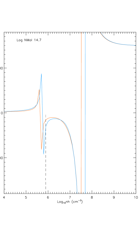
Figure 4.17: Figure shows Excitation Temperature plots for H¹²CN & H¹³CN (1-0) at Log Column Density of 14.7.The intersection of the plots with lognh = 5.9 indicates the values of excitation temperatures for the mean intersection of brightness temperature contours. see Fig. 4.1 The plots show a clear difference between the excitation temperatures of H¹²CN & H¹³CN

Marr et al. (1993) presented a case for the abundance ratio of [HCO⁺]/[HCN] to be proportional to the ratio of their optical depths times the ratio of their Einstein-A coefficients and the assumption that both were optically thick (see Eqn 4.18). They argued that while the determination of the [HCO⁺]/[HCN] ratio was less certain due to their different formation processes, emission from both tracers appeared in the same regions of the CND; and because the HCO⁺(1-0) transition had a similar energy to the HCN(1-0) transition, the HCO⁺ emission should therefore have the same beam filling factor, excitation temperature and background temperature. If this was the case the optically thick brightness temperature for HCO⁺ was the same as for HCN:

$$T(\mathrm{thick},\mathrm{HCO}^{+})\sim T(\mathrm{thick},\mathrm{HCN})=T(\mathrm{H^{12}CN})\,.$$ (4.14)

The optical depth for HCO⁺ was then given by the expression

$$\large{\tau}\normalsize_{\mathrm{HCO}^{+}}=-\ln[1-(\mathrm{T_{HCO^{+}}}/\mathrm{T_{H^{12}CN}})]\,,$$ (4.15)

and Marr et al. (1993) also note that if $\tau$(HCO⁺) $>5$ then

$$\large{\tau}\normalsize(\mathrm{HCO}^{+})\approx\large{\tau}\normalsize(\mathrm{H^{12}CN})\,,$$ (4.16)

and as $\tau$(HCO⁺) cannot be measured with any confidence, it can be inferred that it was optically thick from the fact that $\tau$(H¹²CN) was optically thick. Given that emission from both molecules trace the same gas the ratio of their abundances was related to the ratio of their optical depths via:

$$\frac{[\mathrm{HCO}^{+}]}{[\mathrm{H^{12}CN}]}=\frac{[\large{\tau}\normalsize(\mathrm{HCO}^{+})]}{[\large{\tau}\normalsize(\mathrm{H^{12}CN})]}\times\frac{\mathrm{A}_{21}(\mathrm{H^{12}CN})}{\mathrm{A}_{21}(\mathrm{HCO}^{+})}$$ (4.17)

where A is the molecule’s Einstein A coefficient (2.4 $\times 10^{-5}$ for HCN(1-0) and 5.5 $\times 10^{-5}$ for HCO⁺(1-0)) so that the equation becomes

$$\frac{[HCO^{+}]}{[{H^{12}CN}]}=0.44\times\frac{[\large{\tau}\normalsize(\mathrm{HCO}^{+})]}{[\large{\tau}\normalsize(\mathrm{H^{12}CN})]}\,.$$ (4.18)

Using Eqn 4.18 and the values modelled in Molex for $\tau$(HCO⁺) and $\tau$(H¹²CN) in Table 4.2.2, the [HCO⁺]/[HCN] ratio ranges between 0.4 (Core A) to 0.6 (Core B).

Marr et al. (1993) summarised their results for the [HCO⁺]/[H¹²CN] ratio as varying between 0.1 down to 0.06 with a [C¹²]/[C¹³] value of Z = 30. These [HCO⁺]/[H¹²CN] values were significantly lower than the rates determined from higher resolution observations as between 0.4 and 1.1 (Christopher et al., 2005). The current model used values [HCO⁺]/[H¹²CN] of Z = 0.74 and [H¹²CN]/[H¹³CN] of Z = 11 and produced more credible intersection points for the peak brightness temperature contour plots of the respective molecules than the abundance values adopted in papers by Marr et al. (1993) and Christopher et al. (2005).

Modelling the first core group produced molecular hydrogen densities, between 0.13 and 0.63 $\times 10^{6}$cm^-3 which are lower than for the second core group where the densities are between 0.95 and 1.9 $\times 10^{6}$cm^-3 at a kinetic temperature of T = 150 K and 3.97 $\times 10^{6}$cm^-3 at T = 50 K.

Table 4.4 presents values for the [HCN]/[H₂] ratio for HCN(1-0) in cores A and E in the first group and in cores D and O in the second group from the current modelling results. The effects of varying the core diameters and kinetic temperatures are shown. The ratio ranges between a high of 5$\times 10^{-7}$ and a low of 5$\times 10^{-10}$. The high [HCN]/[H₂] ratios occur for HCN number densities of $20\leq[HCN]\leq 80\times 10^{-4}$cm^-2 arising from either a thick HCN slab or a smaller core size. More typical ratios of of $0.2\leq[HCN]/[H_{2}]\leq 1.2\times 10^{-9}$ result from the second core group analysis where observations have resolved the core sizes.

It should be noted that in their conclusions Christopher et al. (2005) concede that “Some of the HCN emission may be enhanced by shock chemistry implying that estimates of optically thick and optically thin core masses and densities (assuming standard HCN) are overestimates”.

Christopher et al. (2005) mention H¹³CN observations for the NE and SW lobes of the CND and comparison of these with H¹²CN observations support their optically thick scenario, however there are no details provided in their paper to check this scenario.

Greater confidence in the current results would require resolved observation of the CND cores in the HCN (3-2) transition. In spite of this shortcoming, the model analysis of the Marr et al. (1993) cores gives considerable confidence that the HCN gas is optically thin.

The following chapter summarises the work done to present the case for a low hydrogen number density scenario in the CND base on LVG modelling and then lists the conclusions arising from this work.

[ht]

[HCN]/[H${}_{2}]$ Abundance Ratios from Modelled Cores

Core	Kinetic	FWHM	Log HCN	HCN	HCN	Hydrogen	[HCN]/[H2]
Group	Temp	Diameter	Column Density per	Column	Density	Density	Abundance
ID			line width	Density			Ratio
Pairs	(K)	(pc)		($\times 10^{14}$cm-2 km s-1)	($\times 10^{-4}$cm-3)	($\times$106cm-3)	($\times 10^{-9}$)
Firstg
Aa	150	0.43d	13.0	4.45	3.36	0.397	0.85
Bb	150	0.43	13.7	25.06	18.90	0.016	120.00
Aa	150	0.10e	13.0	4.45	14.40	0.397	3.60
Bb	150	0.10	13.7	25.06	81.20	0.016	510.00
Ea	150	0.33d	13.0	8.80	8.64	0.629	1.40
Gb	150	0.10	13.0	8.80	28.50	0.63	450.00
Secondh
Dc	150	0.43	13.3	9.08	6.84	1.26	0.54
Bb	150
Dc	50	0.43	13.4	11.40	8.61	3.96	0.21
Bb	50
Oc	150	0.33d	13.5	8.80	11.54	1.26	0.91
Gb	150
Oc	150	0.25f	13.5	11.54	15.50	1.26	1.20
Gb	150

• H¹²CN(1-0) Marr et al. (1993)

• HCN(3-2) Jackson et al. (1993)

• HCN(1-0) Christopher et al. (2005)

• actual core diameter from Table 2 Christopher et al. (2005)

• average core diameter from Marr et al. (1993)

• average core diameter from Table 2 Christopher et al. (2005)

• core pairs A, H¹²(1-0) & B, HCN(3-2); E, H¹²(1-0) & G, HCN(3-2).

• core pairs D, HCN(1-0) & B, HCN(3-2); O, HCN(1-0)& G, HCN(3-2).

Chapter 5 Summary and Conclusions

The Circumnuclear Disk (CND) is a torus of molecular dust and gas rotating about the galactic centre which has a massive black hole (4$\times$10⁶M_⊙), SgrA^∗. Early observations using different molecules e.g. CO, HCN, NH₃ and CS inferred a low molecular hydrogen density n${}_{H_{2}}\leq$ 10⁶ cm^-3. More recent observations using HCN, HCO⁺, NH₃ and CS (Christopher et al., 2005; Montero-Castaño et al., 2009) infer denser gas n${}_{H_{2}}\geq$ 10⁷ cm^-3 which has led Genzel et al. (2010) to discuss two scenarios and present evidence that supports the lower hydrogen density scenario.

The two scenarios Genzel et al. (2010) used to describe the cores are  :

1. Scenario one considers the gas cores to be cool and sufficiently dense n${}_{H_{2}}\sim$ 10⁷ cm^-3 to be tidally stable leading to an estimated life for the CND of some M yr with the ensuing possibility for star formation within the disk. Evidence supporting this claim is an apparent core stability and the presence of methanol masers near three of the cores (Yusef-Zadeh et al., 2008) that could indicate hot gas flaring from a condensing core in the very early stages of star formation.

2. Scenario two proposes warm, less dense nH${}_{2}\sim$ 10⁶ cm^-3 gas which is tidally unstable leading to a comparatively short disk lifetime of $<$ 10⁵ years and no core condensation. Evidence presented in support of this scenario suggests that the mass of the CND is insufficient (3 to 4 $\times$ 10⁶ M_⊙) to disrupt the orbits of the stellar cluster in the central cavity and there is no evidence of individual dense cores (dark spots) in IR CND images.

The present study sought to reconcile the observations in different HCN transitions in order to identify cores observed in multiple transitions by comparing locations in the CND and kinematic properties (radial velocities). This work was described in Chapter 3 and resulted in the selection of two groups of cores for analysis which is reported in Chapter 4. The LVG model produced hydrogen densities in the CND of n(H₂) = (1–4)$\times$10⁶ cm^-3 with an optically thin, inverted ($\tau$ negative)HCN(1-0) transition that supports the lower hydrogen density scenario.

Data from the twenty-six HCN (1-0) cores listed in Christopher et al. (2005) provided the information for calculating the true (deprojected) core offsets from SgrA^∗, using trial and error to select the disk’s tilt angle, $\alpha$ = 60^∘ out of the plane of the sky. The expression for core model radial velocities was based on the disk’s orientation relative to the plane of the sky and a CND rotational velocity of 110 km s^-1 was adopted to provide a comparison with observed core radial velocities. This comparison illustrated the warped nature of the disk and its composition of circulating gas streamers that rotate at varying velocities. Eighteen of the twenty-six cores fit within the accepted range of disk parameters, while seven cores have radial velocities that are significantly different from the model disk. Variations in the rotational velocity of the disk were discussed in Chapter 1.

The following conclusions are derived from the results presented in this thesis.

The figure of the deprojected HCN (1-0) cores clearly shows the circular structure of the CND with an inner cavity of $\sim$ 1.6 pc. The attempt to fit the HCN(1-0) core radial velocities to the model radial velocity distribution curves demonstrates the warped nature of the disk’s rotating streamers and that the rotational velocity of some streamers vary significantly from the accepted 110 km s^-1.

The LVG modelling of the core group based on Marr et al. (1993) data and the the core group based on more recent data (Christopher et al., 2005; Montero-Castaño et al., 2009) in which the core groups were resolved gave consistent results. Both core groups gave molecular hydrogen number densities that show that the optically thin scenario outlined in Genzel et al. (2010) is more likely than the optically thick scenario proposed by Christopher et al. (2005) and supported by Montero-Castaño et al. (2009). The low molecular hydrogen number densities imply that the cores are not tidally stable and that the disk is a transient structure with a kinematic lifespan of $\sim$ 10⁵ to 10⁶ years which would be too short for star formation and also means that the estimated total mass of the CND could be up to an order of magnitude less than the previous estimate of 10⁶ M_⊙.

The Marr et al. (1993) proposition that excitation temperatures for molecules occupying the same location in the CND is incorrect, the excitation temperatures are indeed different for the prevailing CND conditions and this is why their hypothesis fails.

The discovery of methanol masers by Yusef-Zadeh et al. (2008) in the vicinity of Cores F, G and V may indicate higher hydrogen densities for these cores as a result of a shock mechanism. Those authors proposed that these cores may have condensed to the stage of forming protostars and that the masers are a result of jet outflows from these cores some $10^{4}$ yr after core collapse.

The possibility of a few localised higher density pockets within the CND could be due to either shocks emanating from one or more of the following  : outflows from the young UV stars in the cavity inside the CND, the shock front of the SgrA East SNR and core-core collisions within the CND. Core-core collisions were suggested by Sjouwerman and Pihlström (2008) and Yusef-Zadeh et al. (2001) as the mechanism, which was was formulated by Elitzur (1976) for producing the shocks needed for the formation of 1720 MHz OH masers, which are found in the CND and might be a trigger for star formation.

Greater certainty for the hydrogen density results could be attained if resolved HCN (3-2) transition observations were available for modelling in addition to the currently available (1-0) and (4-3) transition data. The sub millimetre array (SMA) operates at frequencies from 180 to 700 GHz which includes the HCN(3-2) transition frequency of 265.886 GHz. Plans for increasing the sensitivity of this instrument are now in progress (see the SMA Newsletter Number 12, August 2011).

A wider CND survey of the H¹³CN(1-0) transition might clarify the optically thick/thin question and hence the hydrogen density value. An analysis of the NH₃ (1-1), (2-2), (3-3) and (6-6) transitions (Herrnstein and Ho, 2002) would also be useful to check hydrogen densities, particularly as the (6-6) transition traces denser and hotter regions more effectively than HCN. Such a study should be done in the future to reinforce the results of this study.

A possible test of maser effects of negative optical depths in the (1-0) transitions of HCN and HCO⁺ would be to search for a bright (T${}_{b}\sim$ 1000 K) source of continuum emission (such as a quasar or radio galaxy ?) aligned with one of the disk’s cores. A comparison of off HCN line frequency, on line frequency of core observations would then detect an increase in the background intensity caused by amplification of HCN or HCO⁺(1-0) emission as it passes through the core.

The results from this study clearly favour the warm, low density hydrogen gas scenario with a CND mass of 3 to 4 $\times$ 10⁵ M_⊙ and tidal forces pulling the cores apart.

References

- Becklin et al. (1982) E. E. Becklin, I. Gatley, and M. W. Werner. Far-infrared observations of Sagittarius A - The luminosity and dust density in the central parsec of the Galaxy. ApJ, 258:135–142, July 1982.
- Bohlin et al. (1978) R. C. Bohlin, B. D. Savage, and J. F. Drake. A survey of interstellar H I from L-alpha absorption measurements. II. ApJ, 224:132–142, Aug. 1978.
- Christopher et al. (2005) M. H. Christopher, N. Z. Scoville, S. R. Stolovy, and M. S. Yun. HCN and HCO+ Observations of the Galactic Circumnuclear Disk. ApJ, 622:346–365, Mar. 2005.
- Draine and Lee (1984) B. T. Draine and H. M. Lee. Optical properties of interstellar graphite and silicate grains. ApJ, 285:89–108, Oct. 1984.
- Elitzur (1976) M. Elitzur. Inversion of the OH 1720-MHz Line. ApJ, 203:124–131, Jan. 1976.
- Etxaluze et al. (2011) M. Etxaluze, H. A. Smith, V. Tolls, A. A. Stark, and E. Gonzalez-Alfonso. The Galactic Centre in the Far Infrared. ArXiv e-prints 1108.0313, Aug. 2011.
- Genzel (1989) R. Genzel. The Circumnuclear Disk (review). In M. Morris, editor, The Center of the Galaxy, volume 136 of IAU Symposium, pages 393–405, 1989.
- Genzel et al. (2010) R. Genzel, F. Eisenhauer, and S. Gillessen. The Galactic Center massive black hole and nuclear star cluster. Reviews of Modern Physics, 82:3121–3195, Oct. 2010.
- Guesten et al. (1987) R. Guesten, R. Genzel, M. C. H. Wright, D. T. Jaffe, J. Stutzki, and A. I. Harris. Aperture synthesis observations of the circumnuclear ring in the Galactic center. ApJ, 318:124–138, July 1987.
- Harris et al. (1985) A. I. Harris, D. T. Jaffe, M. Silber, and R. Genzel. CO 7-6 submillimeter emission from the galactic center - Warm molecular gas and the rotation curve in the central 10 parsecs. ApJ, 294:L93–L97, July 1985.
- Herrnstein and Ho (2002) R. M. Herrnstein and P. T. P. Ho. Hot Molecular Gas in the Galactic Center. ApJ, 579:L83–L86, Nov. 2002.
- Jackson et al. (1993) J. M. Jackson, N. Geis, R. Genzel, A. I. Harris, S. Madden, A. Poglitsch, G. J. Stacey, and C. H. Townes. Neutral gas in the central 2 parsecs of the Galaxy. ApJ, 402:173–184, Jan. 1993.
- Karlsson et al. (2003) R. Karlsson, L. O. Sjouwerman, A. Sandqvist, and J. B. Whiteoak. 18-cm VLA observations of OH towards the Galactic Centre. Absorption and emission in the four ground-state OH lines. A&A, 403:1011–1021, June 2003.
- Liszt et al. (1985) H. S. Liszt, W. B. Burton, and J. M. van der Hulst. Associations between neutral and ionized gas in SGR A. A&A, 142:237–244, Jan. 1985.
- Lockett and Elitzur (1989) P. Lockett and M. Elitzur. An escape probability treatment of line fluorescence and overlap in astrophysics. ApJ, 344:525–530, Sept. 1989.
- Mangum et al. (1988) J. G. Mangum, R. T. Rood, E. J. Wadiak, and T. L. Wilson. Observations of the C-13 isomers of cyanoacetylene - Implications for carbon isotope studies in the Milky Way. ApJ, 334:182–190, Nov. 1988.
- Marr et al. (1993) J. M. Marr, M. C. H. Wright, and D. C. Backer. HCO+, H13CN and H12CN aperture synthesis observations of the circumnuclear ring in the Galactic center. ApJ, 411:667–673, July 1993.
- Marshall et al. (1995) J. Marshall, A. N. Lasenby, and A. I. Harris. HCN observations of the circumnuclear disc in the Galactic Centre. MNRAS, 277:594–608, Nov. 1995.
- Mehringer and Menten (1997) D. M. Mehringer and K. M. Menten. 44 GHz Methanol Masers and Quasi-thermal Emission in Sagittarius B2. ApJ, 474:346–361, Jan. 1997.
- Mezger et al. (1989) P. G. Mezger, R. Zylka, C. J. Salter, J. E. Wink, R. Chini, E. Kreysa, and R. Tuffs. Continuum observations of SGR A at mm/submm wavelengths. A&A, 209:337–348, Jan. 1989.
- Mezger et al. (1996) P. G. Mezger, W. J. Duschl, and R. Zylka. The Galactic Center: a laboratory for AGN? A&A Rev., 7:289–388, 1996.