A Method for Geometry Optimization in a Simple Model of Two-Dimensional Heat Transfer

Abstract

This investigation is motivated by the problem of optimal design of cooling elements in modern battery systems. We consider a simple model of two-dimensional steady-state heat conduction described by elliptic partial differential equations and involving a one-dimensional cooling element represented by a contour on which interface boundary conditions are specified. The problem consists in finding an optimal shape of the cooling element which will ensure that the solution in a given region is close (in the least squares sense) to some prescribed target distribution. We formulate this problem as PDE-constrained optimization and the locally optimal contour shapes are found using a gradient-based descent algorithm in which the Sobolev shape gradients are obtained using methods of the shape-differential calculus. The main novelty of this work is an accurate and efficient approach to the evaluation of the shape gradients based on a boundary-integral formulation which exploits certain analytical properties of the solution and does not require grids adapted to the contour. This approach is thoroughly validated and optimization results obtained in different test problems exhibit nontrivial shapes of the computed optimal contours.

Keywords: heat transfer, adjoint-based optimization, shape calculus, Sobolev gradients, boundary integral equations

AMS subject classifications: 80M50, 35Q93, 49Q10, 49Q12, 65N38

1 Introduction

1.1 Motivation

The goal of this investigation is to develop and validate a computational method for optimization of the shape of cooling elements in general steady heat transfer problems. The motivation for this work comes from problems encountered in the design of battery systems for hybrid-electric (HEV) and electric vehicles (EV) [1] in which a central role is played by methods of the thermal battery management (TMB) ensuring that the battery operates in a suitable thermal environment [2]. A typical battery system used in automotive applications is shown in Figure 1a, whereas in Figure 1b we present a possible design of the channels with the coolant fluid acting as the heat-exchange elements. In these applications a key issue is optimization of the shape of the cooling elements, so that the temperature distribution is as close as possible to prescribed profiles in some selected regions of the battery system. Assuming a known distribution of the heat sources representing the heat generation in the battery, mathematical models of such problems lead to systems of elliptic boundary-value problems defined on irregular domains and subject to some rather complicated boundary conditions. Optimization of geometry of the cooling elements thus leads to shape-optimization problems for such systems of equations, and in this study we propose an approach based on the continuous (i.e., infinite-dimensional, or “optimize-then-differentiate”, [3]) formulation and the methods of the shape-differential calculus. The main novel contribution is the development and validation of an accurate and efficient technique based on the boundary-integral formulation for the evaluation of the shape gradients which is a key enabler of the proposed optimization strategy.

  

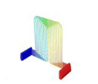
Figure 1: (a) Battery system used in hybrid-electric vehicles and (b) possible design of the cooling elements (courtesy of General Motors of Canada).

In the literature devoted to heat transfer and the related field of fluid mechanics most of the works concerning shape optimization, or equivalently shape identification, concern problems formulated in the “discretize-then-differentiate” setting, where a finite-dimensional optimization problem is set up based on a discrete version of the governing equations, somewhat limiting the flexibility in dealing with different geometries. Such approaches were pursued, for example, in [4, 5, 6, 7, 8, 9], and we also mention the monograph [10]. Approaches based on continuous adjoint formulations usually rely on the shape-differential calculus to determine the shape sensitivities. The shape calculus, reviewed in the monographs [11, 12, 13], is a general suite of techniques derived from differential geometry which allow one to differentiate solutions of partial differential equations (PDEs) and functionals defined on these solutions with respect to variations of the domains on which these PDEs are defined. Applications of various continuous shape-optimization approaches to problems involving heat transfer, fluid flow and phase transformations were investigated in [14, 15, 16, 17, 18, 19, 20, 21]. We add that, as regards the numerical representation of free boundaries in PDE problems, there are two main computational approaches, namely, the “interface capturing” methods based on the use of suitable implicit functions, such as the level set formulation [22], and the “interface tracking” methods which rely on explicit representations of the boundary. Since the model problem considered here is described by elliptic PDEs, we survey below the state-of-the-art numerical techniques used for the solution of optimization problems for such system based on the continuous formulation.

1.2 Review of Computational Methods for Shape Optimization of Elliptic PDEs

In both paradigms, i.e., in the approaches relying on the level sets to capture the interface and in the methods based on explicit interface tracking, optimization problems are typically solved using discrete (with respect to some pseudo-time) forms of gradient flows in which suitably defined shape gradients are used as the descent directions. Starting with the seminal work [23], most attention has recently been focused on level-set-based techniques in which the level-set function is evolved using the Hamilton-Jacobi equation with the velocity field given as an extension of the shape gradient away from the interface. Their advantage is that they do not require interface-fitted domain discretizations and perform well on simple Cartesian grids. The governing and adjoint problems can be solved using the immersed interface method [24], as was done for example in [25, 26], or with a penalization technique [27]. Regularization aspects of such approaches were investigated in [28], whereas the study [29] explored formulations resulting from different definitions of the inner products for the shape variations. Limitations of such methods arise when the boundary conditions and/or the shape gradients defined on the interface have a more complicated form (e.g., include derivatives), as then they tend to be difficult to evaluate accurately on Cartesian grids. On the other hand, shape optimization techniques based on explicit interface tracking typically require interface-fitted discretization of the domains on which the governing and adjoint systems are solved. This discretization then needs to be updated during iterations which can be a complicated process. Such approaches were reviewed in [30], whereas some applications to image processing are discussed in [31, 32]

The approach proposed here is based on explicit interface tracking combined with suitably chosen Sobolev gradients. While both the shape-differentiation and Sobolev gradients are well-known techniques, the main novelty of the proposed approach is a method for the evaluation of shape gradients which is based on a boundary-integral formulation coupled with an elliptic solver constructed using a Cartesian grid. In comparison to the approaches described above, it offers the following advantages

• it is characterized by a high (in principle spectral) accuracy in approximating complex interface boundary conditions and expressions for the shape gradients, so that only modest resolution is required to discretize the contour,

• as boundary-fitted grids need not be constructed, it can deal with fairly complicated contour shapes at a low computational cost.

The proposed implementation takes advantage of the analytic structure of the governing equations. While boundary-integral techniques have been used for shape optimization of elliptic PDEs, this was typically done in the discrete setting (i.e., “discretize-then-differentiate”) with or without the adjoint equations used to evaluate the shape sensitivities as in [33, 34, 35, 36, 37, 38]. In [39] the optimized shape was described in terms of a graph of a function, so that determination of the gradients did not require methods of the shape-differential calculus. A boundary-integral formulation for a time-dependent (parabolic) shape optimization problem was devised in [40]. We add that all of these approaches relied on the standard techniques of the boundary-element method (BEM) to evaluate the resulting integral expressions. Finally, we also mention [41] and some references cited therein where the shape sensitivities were expressed in terms of hypersingular integral equations (obtained via shape-differentiation of the standard boundary-integral formulations). We will comment on this interesting alternative approach at the end of the paper.

The structure of the paper is as follows: in the next Section we introduce the mathematical model of the system and state the optimization problem, in the following Section we briefly describe a gradient-based descent algorithm based on shape-differentiation and smoothed (Sobolev) gradients; the proposed computational method for the solution of the governing and adjoint system and evaluation of the sensitivities is presented in detail in Section 4, whereas validation tests and results demonstrating application of the method to some selected shape optimization problems are presented in Section 5; discussion and conclusions are deferred to Section 6.

2 Mathematical Model and Optimization Problem

We will consider a simplified model of the problem based on the following set of assumptions

Assumptions 1

1. heat transfer is independent of time and occurs via conduction only with $k>0$ representing the constant thermal conductivity,

2. the battery pack is treated as a 2D square region $\Omega\subset{\mathbb{R}}^{2}$ with isolated boundary $\partial\Omega$ (i.e., the heat flux vanishes on $\partial\Omega$),

3. the distribution of the heat sources in the battery is given by the function $q\;:\;\Omega\rightarrow{\mathbb{R}}$ which we will assume to be square-integrable, i.e., $q\in L_{2}(\Omega)$; the corresponding temperature distribution will be denoted by $u\;:\;\Omega\rightarrow{\mathbb{R}}$,

4. the cooling element is represented by a $C^{1}$ curve ${\mathcal{C}}$ of total length $L=\oint_{{\mathcal{C}}}\,ds$ and characterized by the reference temperature $u_{0}$; the density $w$ of the heat flux absorbed by the cooling element at a point ${\mathbf{x}}_{{\mathcal{C}}}\in{\mathcal{C}}$ is modelled using Newton’s law of cooling as $w=\gamma(u|_{{\mathcal{C}}}-u_{0})$, where $\gamma>0$ is a constant heat transfer coefficient and the temperature field $u$ is continuous across the contour ${\mathcal{C}}$,

5. given an arbitrary subdomain ${\mathcal{A}}\subseteq\Omega$, the target temperature distribution is given by ${\overline{u}}\;:\;{\mathcal{A}}\longrightarrow{\mathbb{R}}$.

    

Figure 2: Sketch of the domain $\Omega$ with the target region ${\mathcal{A}}$ for (a) Problem P1 with a closed contour ${\mathcal{C}}$ and (b) Problem P2 with an open contour ${\mathcal{C}}$ representing the cooling element.

We restrict our attention to contours which are Lipschitz-continuous and will assume that they are parameterized in terms of the arc-length coordinate $s\in[0,L]$. Two versions of the problem will be considered:

$$\begin{aligned} \textrm{P1:}\ \ &{\mathbf{x}}_{{\mathcal{C}}}\big{|}_{s=0}={\mathbf{x}}_{{\mathcal{C}}}\big{|}_{s=L}\notin\partial\Omega,\\ &u_{0}=\textrm{Const}\end{aligned}\quad\begin{aligned} \textrm{P2:}\ \ &{\mathbf{x}}_{{\mathcal{C}}}\big{|}_{s=0},{\mathbf{x}}_{{\mathcal{C}}}\big{|}_{s=L}\in\partial\Omega,\ {\mathbf{x}}_{{\mathcal{C}}}\big{|}_{s=0}\neq{\mathbf{x}}_{{\mathcal{C}}}\big{|}_{s=L}\\ &u_{0}=u_{0}(s)\end{aligned}$$ (1)

corresponding, respectively, to a closed contour ${\mathcal{C}}$ with a constant reference temperature and to an open contour ${\mathcal{C}}$ with the reference temperature $u_{0}=u_{0}(s)$ varying with the arc length. All validation tests and a number of optimizations will be performed for the simper problem P1. In addition, some optimization problems will be solved for the more realistic configuration P2 in which $q$ will be taken to be the distribution of the heat sources in an actual battery (Figure 1b). To fix attention, in Problem P2 we will assume that $u_{0}$ increases linearly with the length corresponding to the coolant liquid heating up as it absorbs heat, i.e.,

$$u_{0}(s)=T_{a}+\frac{T_{b}-T_{a}}{L}\,s,\quad s\in[0,L],$$ (2)

where $T_{a}$ and $T_{b}$ are the prescribed temperatures at the inlet and outlet. Sketches of the domain $\Omega$ with its different attributes are shown for both cases in Figure 2. In Problem P2 with an open contour ${\mathcal{C}}$ the endpoints are assumed to attach to the domain boundary at the right angles. We will denote $\Omega_{1}$ the part of the domain $\Omega$ inside, or above, contour ${\mathcal{C}}$, and $\Omega_{2}\triangleq\Omega\backslash\overline{\Omega}_{1}$ its complement, cf. Figure 2 (“$\triangleq$” means “equal to by definition”). Denoting $u_{1}\triangleq u|_{\Omega_{1}}$ and $u_{2}\triangleq u|_{\Omega_{2}}$ the restrictions of the temperature field to the subdomains on the two sides of contour ${\mathcal{C}}$, we have the following mathematical model of the problem

$$-k\,\Delta u_{1} =q\quad \textrm{in}\ \Omega_{1},$$ (3a)

$$-k\,\Delta u_{2} =q\quad \textrm{in}\ \Omega_{2},$$ (3b)

$$u_{2} =u_{1}\left(\triangleq u|_{{\mathcal{C}}}\right)\quad \textrm{on}\ {\mathcal{C}},$$ (3c)

$$k\,\left({\partial u_{2}\over\partial n}-{\partial u_{1}\over\partial n}\right) =\gamma\,(u_{1}-u_{0})\quad \textrm{on}\ {\mathcal{C}},$$ (3d)

$$k\,{\partial u\over\partial n} =0\quad \textrm{on}\ \partial\Omega,$$ (3e)

where ${\mathbf{n}}$ is the unit vector normal to the contour ${\mathcal{C}}$, or the boundary $\partial\Omega$, and oriented as shown in Figure 2. The corresponding unit tangent vector will be denoted ${\mathbf{t}}$. We add that boundary conditions (3c) and (3d) represent Newton’s law of cooling mentioned in Assumption 1.(iv). Typically used to model the heat transfer in the presence of convection, this law stipulates that the heat flux $k\left({\partial u_{2}\over\partial n}-{\partial u_{1}\over\partial n}\right)|_{{\mathbf{x}}_{{\mathcal{C}}}}$ absorbed into the cooling element ${\mathcal{C}}$ at a given point ${\mathbf{x}}_{{\mathcal{C}}}\in{\mathcal{C}}$ is proportional to the difference between the local temperature $u|_{{\mathbf{x}}_{{\mathcal{C}}}}$ and the reference temperature $u_{0}$. We remark that $u_{0}$ may be therefore thought of as the temperature of some hypothetical coolant liquid circulating in the cooling element, although details of this process are neglected in the present model (the contour ${\mathcal{C}}$ has in fact zero thickness). Clearly, the solution $u$ will depend on the shape of the contour, i.e., $u=u({\mathcal{C}})$. We also remark that, while the differential equations and boundary conditions in system (3) are linear in the dependent variables $u_{1}$ and $u_{2}$, problem (3) is in fact geometrically nonlinear with respect to the shape of the contour ${\mathcal{C}}$. For a discussion of the existence and regularity of solutions to elliptic boundary-value problems in complicated domains we refer the reader to monograph [42].

The optimization problem, motivated by the industrial applications discussed in Introduction, is to find an optimal contour $\tilde{{\mathcal{C}}}$ such that the corresponding solution $\tilde{u}\triangleq u(\tilde{{\mathcal{C}}})$ of system (3) evaluated over ${\mathcal{A}}$ is as close as possible to the prescribed target distribution ${\overline{u}}$. Defining the reduced least-squares cost functional as

$${\mathcal{J}}({\mathcal{C}})\triangleq\frac{1}{2}\int_{A}(u-\overline{u})^{2}\,d\Omega,$$ (4)

we obtain the following optimization problem

$$\min_{{\mathcal{C}}}{\mathcal{J}}({\mathcal{C}})$$ (5)

$$\textrm{subject to System}\ \eqref{eq:intr_d}.$$

Since in actual applications the length of the contour representing the cooling element may not be arbitrary, we will also consider a second optimization problem with the additional constraint on the contour length, namely,

$$\min_{{\mathcal{C}}}{\mathcal{J}}({\mathcal{C}})$$ (6)

subject to: $$\textrm{System}\ \eqref{eq:intr_d}$$

$$\oint_{{\mathcal{C}}}\,ds=L_{0},$$

where $L_{0}>0$ is the prescribed length of the contour $\tilde{{\mathcal{C}}}$. Clearly, problems (5) and (6) represent PDE-constrained shape optimization problems. PDE optimization problems involving shapes of the domains as the control variables require special treatment [11, 12, 13], and our computational approach will be based on methods of the shape-differential calculus recalled in the next Section. Finally, we add that, in principle, in the statement of optimization problems (5) and (6) we should also include the condition ${\mathcal{C}}\subset\Omega$ which is equivalent to a suitable set of inequality constraints. However, in the interest of simplifying the formulation, this condition is omitted here, although as discussed in Section 3 below, it will be incorporated in the final computational algorithm.

3 Gradient-Based Minimization Approach

In this Section we review the formulation of the optimality conditions for problems (5) and (6) and a gradient-based descent approach for the computational solution of these problems. Since these elements of our approach are rather standard, their presentation will be brief. We consider the first-order optimality conditions which require the vanishing of a suitably-defined Gâteaux (directional) differential evaluated at the optimal contour $\tilde{{\mathcal{C}}}$. We remark that defining such differential and the related expression for the gradient requires differentiation of governing system (3) with respect to the shape of the domains $\Omega_{1}$ and $\Omega_{2}$ on which the PDEs are defined. This is properly done based on the methods of the shape-differential calculus [11, 12] which rely on a special parametrization of the domain geometry and provide formulas for shape-differentiation of general functionals, PDEs and the associated boundary conditions. Below we briefly present this construction and recall the main results we will need, referring the reader to monographs [12, 13] for further details. As a first step, we define the “velocity” field ${\mathbf{V}}\;:\;\Omega\to{\mathbb{R}}^{2}$ which will parametrize the deformations of the contour ${\mathcal{C}}$ and of the domains $\Omega_{1}$ and $\Omega_{2}$, so that for every point ${\mathbf{x}}_{\mathcal{C}}\in{\mathcal{C}}$ we have

$${\mathbf{x}}_{{\mathcal{C}}(\epsilon)}={\mathbf{x}}_{\mathcal{C}}+\epsilon{\mathbf{V}},$$ (7)

where $0<\epsilon\ll 1$ is a parameter and ${\mathbf{x}}_{{\mathcal{C}}(\epsilon)}$ is the position of a point on the deformed contour ${\mathcal{C}}(\epsilon)$. Relations analogous to (7) can also be written for points in the deformed domains $\Omega_{1}(\epsilon)$ and $\Omega_{2}(\epsilon)$. Given a sufficiently regular function $\psi\;:\;\Omega\to{\mathbb{R}}$ and the functionals $j_{1}(\Omega_{1}(\epsilon))\triangleq\int_{\Omega_{1}(\epsilon)}\psi({\mathbf{x}};\Omega_{1}(\epsilon))\,d\Omega$ and $j_{2}({\mathcal{C}}(\epsilon))\triangleq\int_{{\mathcal{C}}(\epsilon)}\psi({\mathbf{x}};{\mathcal{C}}(\epsilon))\,ds$ defined on the perturbed domain and contour, the corresponding shape differentials are defined as $j^{\prime}_{1}(\Omega_{1};{\mathbf{V}})\triangleq\lim_{\epsilon\to 0}\epsilon^{-1}[j_{1}(\Omega_{1}(\epsilon))-j_{1}(\Omega_{1}(0))]$ and $j^{\prime}_{2}({\mathcal{C}};{\mathbf{V}})\triangleq\lim_{\epsilon\to 0}\epsilon^{-1}[j_{2}({\mathcal{C}}(\epsilon))-j_{2}({\mathcal{C}}(0))]$. One of the central results of the shape-differential calculus is summarized in the following

Lemma 1

The shape differentials of $j_{1}(\Omega_{1})$ and $j_{2}({\mathcal{C}})$ with respect to parametrization (7) are given by expressions

$$j^{\prime}_{1}(\Omega_{1};{\mathbf{V}}) =\int_{\Omega_{1}}\psi^{\prime}\,d\Omega+\oint_{{\mathcal{C}}}\psi\,(\boldsymbol{{\mathbf{V}}}\cdot{\mathbf{n}})\,ds,$$ (8a)

$$j^{\prime}_{2}({\mathcal{C}};{\mathbf{V}}) =\oint_{{\mathcal{C}}}\psi^{\prime}\,d{\mathbf{s}}+\oint_{{\mathcal{C}}}\left({\partial\psi\over\partial n}+\kappa\,\psi\right)(\boldsymbol{{\mathbf{V}}}\cdot{\mathbf{n}})\,ds,$$ (8b)

where $\psi^{\prime}$ is the shape derivative of the integrand function $\psi$ defined for $\forall{\mathbf{x}}\in\Omega$ as $\psi^{\prime}({\mathbf{x}})\triangleq\lim_{\epsilon\rightarrow 0}\epsilon^{-1}\left[\psi({\mathbf{x}};\Omega_{1}(\epsilon))-\psi({\mathbf{x}};\Omega_{1}(0))\right]$ and $\kappa$ denotes the signed curvature of the contour ${\mathcal{C}}$.

A detailed proof of Lemma 1 can be found, for example, in [12]. We remark that, in general, when differentiating with respect to the shape of open contours, expressions (8a) and (8b) will have additional terms proportional to $({\mathbf{V}}\cdot{\mathbf{t}})$ and localized via Dirac delta distributions at the contour endpoints [43, 18]. However, in our Problem P2, owing to (1) and the assumption that contour ${\mathcal{C}}$ meets the domain boundary $\partial\Omega$ at the right angle (cf. Figure 2b), these terms vanish identically. Therefore, for both the closed and open contours only the normal component $\zeta\triangleq({\mathbf{V}}\cdot{\mathbf{n}})|_{\mathcal{C}}$ of the perturbation velocity field on the contour ${\mathcal{C}}$ plays a role in expressions for shape differentials (8). The normal perturbations $\zeta=\zeta(s)$, considered as functions of the arc-length coordinate, must satisfy certain regularity conditions. It is sufficient for the perturbation $\zeta$ to belong to the Sobolev space $H^{1}(0,L)$ of periodic functions with square-integrable derivatives on $[0,L]$ (precise definition of the corresponding inner product will be given in (17) below). We add that contour parametrization allows us to recast line integrals, such as appearing in (8a), (8b) and below, as definite integrals.

The optimality condition for problem (5) is given by

$$\forall_{\zeta\in H^{1}(0,L)}\quad{\mathcal{J}}^{\prime}(\tilde{{\mathcal{C}}};\zeta{\mathbf{n}})=\int_{{\mathcal{A}}}(u-{\overline{u}})\,u^{\prime}\,d\Omega=0,$$ (9)

where we note that the subdomain ${\mathcal{A}}$ is fixed and does not depend on the perturbation $\zeta$, and $u^{\prime}=u^{\prime}(\tilde{{\mathcal{C}}},\zeta{\mathbf{n}})$ is the shape derivative of the solution of governing problem (3) evaluated for the optimal contour shape $\tilde{{\mathcal{C}}}$. The sensitivity (perturbation) equation satisfied by $u^{\prime}$ is obtained by considering a suitable weak form of system (3) and shape-differentiating the resulting integrals using formulas (8), see [13],

$$k\,\Delta u^{\prime}_{1} =0\quad \text{in}\ \Omega_{1},$$ (10a)

$$k\,\Delta u^{\prime}_{2} =0\quad \text{in}\ \Omega_{2},$$ (10b)

$$u^{\prime}_{2}-u^{\prime}_{1} =\left({\partial u_{1}\over\partial n}-{\partial u_{2}\over\partial n}\right)\zeta\quad \text{on}\ {\mathcal{C}},$$ (10c)

$$k\,\left({\partial u^{\prime}_{2}\over\partial n}-{\partial u^{\prime}_{1}\over\partial n}\right)-\gamma\,u^{\prime}_{1} =\gamma\,\left[{\partial u_{1}\over\partial n}+\kappa\,(u_{1}-u_{0})\right]\zeta{-\gamma\,u^{\prime}_{0}}\quad \text{on}\ {\mathcal{C}},$$ (10d)

$$k{\partial u^{\prime}\over\partial n} =0\quad \text{on}\ \partial\Omega,$$ (10e)

where $u^{\prime}_{1}\triangleq u^{\prime}|_{\Omega_{1}}$ and $u^{\prime}_{2}\triangleq u^{\prime}|_{\Omega_{2}}$, and $u^{\prime}_{0}$ is the shape-derivative of (2)

$$u^{\prime}_{0}=u^{\prime}_{0}(s;\zeta{\mathbf{n}})=\frac{T_{b}-T_{a}}{L}\int_{0}^{L}\left[H(s-s^{\prime})-s/L\right]\kappa\zeta\,ds^{\prime}$$ (11)

in which $H(\cdot)$ is the Heaviside function and whose structure is a consequence of the dependence of the arc length $s=s({\mathcal{C}})$ on the contour shape. As a matter of course, in problem P1, $u^{\prime}_{0}\equiv 0$, cf (1).

As regards the second optimization problem (6), we will incorporate the additional constraint on the length of the contour ${\mathcal{C}}$ by defining an augmented cost functional

$${\mathcal{J}}_{\alpha}({\mathcal{C}})\triangleq{\mathcal{J}}({\mathcal{C}})+\frac{\alpha}{2}\left(\int_{{\mathcal{C}}}\,ds-L_{0}\right)^{2},$$ (12)

where $\alpha>0$ is a numerical parameter. The optimality condition for this second optimization problem is thus

$$\forall_{\zeta\in H^{1}(0,L)}\quad{\mathcal{J}}^{\prime}_{\alpha}(\tilde{{\mathcal{C}}};\zeta{\mathbf{n}})=\int_{{\mathcal{A}}}(u-{\overline{u}})u^{\prime}\,d\Omega+\alpha\left(\int_{\tilde{{\mathcal{C}}}}\,ds-L_{0}\right)\oint_{\tilde{{\mathcal{C}}}}\kappa\zeta\,ds=0,$$ (13)

where we used relationship (8b) to differentiate the second term in (12). We note that, although it arises from rather different mathematical principles, the more systematic formulation of the constrained problem using Lagrange multipliers would result in an optimality condition quite similar to (13). More precisely, the only difference is that the factor $\alpha\left(\int_{\tilde{{\mathcal{C}}}}\,ds-L_{0}\right)$ in (13) would be replaced by the Lagrange multiplier $\lambda$. As a result, the modification of the descent direction would have the same form (but with a different magnitude) in the two cases. On the other hand, given the geometric nonlinearity of the constraint $\int_{\tilde{{\mathcal{C}}}}\,ds=L_{0}$, the Lagrange multiplier $\lambda$ can be rather hard to compute accurately, so for simplicity in this study we chose formulation (12)–(13). We emphasize that optimality conditions (9) and (13) only characterize local, rather than global, minimizers and due to the non-convexity of cost functional (4), resulting from the geometric nonlinearity of system (3) and the length constraint, existence of multiple local minima can be expected. The (locally) optimal shape $\tilde{{\mathcal{C}}}$ can be found computationally as ${\mathbf{x}}_{\tilde{{\mathcal{C}}}}=\lim_{n\to\infty}{\mathbf{x}}_{{\mathcal{C}}^{(n)}}$ using the following gradient-descent algorithm

$${\mathbf{x}}_{{\mathcal{C}}^{(n+1)}} ={\mathbf{x}}_{{\mathcal{C}}^{(n)}}-\tau_{n}\boldsymbol{\nabla}{\mathcal{J}}\left({\mathcal{C}}^{(n)}\right),\qquad n=1,2,\dots,$$ (14)

$${\mathbf{x}}_{{\mathcal{C}}^{(0)}} ={\mathbf{x}}_{{\mathcal{C}}_{0}},$$

where the points ${\mathbf{x}}_{{\mathcal{C}}_{0}}$ represent the contour ${\mathcal{C}}_{0}$ used as the “initial guess” and $\tau_{n}$ is the length of the step along the descent direction at the $n$-th iteration computed by solving a line-minimization problem

$$\tau_{n}=\operatorname{argmin}_{\tau>0}\{{\mathcal{J}}({\mathcal{C}}^{(n)}-\tau\,\boldsymbol{\nabla}{\mathcal{J}}({\mathcal{C}}^{(n)})\}.$$ (15)

There are many different approaches to solving problems of this type and in our study we use Brent’s iterative method combining the golden section search with inverse parabolic interpolation in the neighbourhood of the minimum. This approach does not require any derivatives with respect to $\tau$ and an efficient implementation is discussed in [44]. If $\tau_{n}$ found by solving problem (15) results in the deformed contour ${\mathcal{C}}^{(n+1)}$ intersecting the domain boundary $\partial\Omega$, the value of $\tau_{n}$ is suitably reduced to ensure the condition ${\mathcal{C}}^{(n+1)}\subset\Omega$ is always satisfied. We add that, while for the sake of brevity of notation formula (14) represents the steepest descent approach, more advanced optimization methods such as the Polak-Ribiére version of the nonlinear conjugate gradients method [45] were used to obtain the results presented in Section 5.2. At least for the problems we investigated, these approaches were found to systematically outperform the steepest descent method. Clearly, a critical element of minimization algorithm (14) is evaluation at every iteration of the cost functional gradient $\boldsymbol{\nabla}{\mathcal{J}}({\mathcal{C}}^{(n)})$. The Riesz representation theorem [46] guarantees that it can be extracted from the Gâteaux shape differential according to the formula

$${\mathcal{J}}^{\prime}({\mathcal{C}};\zeta{\mathbf{n}})=\Big{\langle}\boldsymbol{\nabla}^{H^{1}}{\mathcal{J}}({\mathcal{C}}),\zeta\Big{\rangle}_{H^{1}(0,L)},$$ (16)

where

$$\big{\langle}z_{1},z_{2}\big{\rangle}_{H^{1}(0,L)}=\int_{0}^{L}z_{1}z_{2}+\ell^{2}{\partial z_{1}\over\partial s}{\partial z_{2}\over\partial s}\,ds,\quad\forall_{z_{1},z_{2}\in{H^{1}(0,L)}}$$ (17)

denotes an inner product in the Sobolev space $H^{1}(0,L)$ in which $\ell\in{\mathbb{R}}$ is a parameter (which will be shown below to have the meaning of a length scale). We observe that expressions for the Gâteaux differentials ${\mathcal{J}}^{\prime}({\mathcal{C}};\zeta{\mathbf{n}})$ and ${\mathcal{J}}^{\prime}_{\alpha}({\mathcal{C}};\zeta{\mathbf{n}})$ appearing in (9) and (13) are not yet in the form consistent with (16), because the perturbation $\zeta$ rather than appear as a factor is hidden in boundary conditions (10c)–(10d) of the sensitivity system defining $u^{\prime}$. In order to transform the differential ${\mathcal{J}}^{\prime}({\mathcal{C}};\zeta{\mathbf{n}})$ to Riesz form (16) we will employ the adjoint variable $u^{*}\;:\;\Omega\to{\mathbb{R}}$ which is the solution of the following adjoint system

$$-k\,\Delta u^{*}_{1} =(u-\overline{u})\chi_{A_{1}}\quad \text{in}\ \Omega_{1},$$ (18a)

$$-k\,\Delta u^{*}_{2} =(u-\overline{u})\chi_{A_{2}}\quad \text{in}\ \Omega_{2},$$ (18b)

$$u^{*}_{2}-u^{*}_{1} =0\quad \text{on}\ {\mathcal{C}},$$ (18c)

$$k\,\left({\partial u^{*}_{2}\over\partial n}-{\partial u^{*}_{1}\over\partial n}\right) =\gamma\,u^{*}_{1}\quad \text{on}\ {\mathcal{C}},$$ (18d)

$${\partial u^{*}\over\partial n} =0\quad \text{on}\ \partial\Omega,$$ (18e)

where $u^{*}_{1}\triangleq u^{*}|_{\Omega_{1}}$ and $u^{*}_{2}\triangleq u^{*}|_{\Omega_{2}}$, whereas $\chi_{{\mathcal{A}}_{i}}$ is the characteristic function of the region ${\mathcal{A}}_{i}\triangleq\Omega_{i}\bigcap{\mathcal{A}}$, $i=1,2$. Following the standard procedure, see e.g. [3], we obtain

$${\mathcal{J}}^{\prime}({\mathcal{C}};\zeta{\mathbf{n}})=\int_{0}^{L}\boldsymbol{\nabla}^{L_{2}}{\mathcal{J}}\zeta\,ds,$$ (19)

where

$$\boldsymbol{\nabla}^{L_{2}}{\mathcal{J}}= -\gamma\,(u_{1}-u_{0})\left(\kappa\,u^{*}_{1}+{\partial u^{*}_{1}\over\partial n}\right)-\gamma\,u^{*}_{1}{\partial u_{2}\over\partial n}$$ (20)

$${-\gamma\,\kappa\,\frac{T_{b}-T_{a}}{L}\int_{0}^{L}\left[H(s^{\prime}-s)-s^{\prime}/L\right]u^{*}(s^{\prime})\,ds^{\prime}}\qquad\text{on}\ {\mathcal{C}}.$$

The last term in (20) stems from the arc length dependence of the reference temperature $u_{0}$ in Problem P2, cf. (2), and vanishes identically in Problem P1. Derivation details are presented in [47, 48]; in [47] we also discuss a symbolic algebra algorithm for automated determination of the adjoint boundary conditions in PDE optimization problems characterized by complicated interface conditions such as the problem considered here. While this is not the gradient we use in the actual computations, for simplicity in (19)–(20) the gradient $\boldsymbol{\nabla}^{L_{2}}{\mathcal{J}}$ was obtained as the Riesz representer in the space $L_{2}(0,L)$ of square-integrable functions. We also add that the part of Gâteaux differential (13) associated with the length constraint is already in the Riesz form, so that the $L_{2}$ gradient of cost functional ${\mathcal{J}}_{\alpha}({\mathcal{C}})$ is

$$\boldsymbol{\nabla}^{L_{2}}{\mathcal{J}}_{\alpha}=\boldsymbol{\nabla}^{L_{2}}{\mathcal{J}}+\alpha\,\left(\int_{{\mathcal{C}}}\,ds-L_{0}\right)\kappa\,\quad\text{on}\ {\mathcal{C}}.$$ (21)

The gradients actually used in minimization algorithm (14), namely the Sobolev gradients $\boldsymbol{\nabla}^{H^{1}}{\mathcal{J}}$ and $\boldsymbol{\nabla}^{H^{1}}{\mathcal{J}}_{\alpha}$, can be obtained from (20) and (21) by identifying (16)–(17) with (19), and noting the arbitrariness of the shape perturbations $\zeta\in H^{1}(0,L)$. Then, after integrating by parts and using the boundary conditions, we arrive at

$$\left(1-\ell^{2}\,{\partial^{2}\over\partial s^{2}}\right)\,\boldsymbol{\nabla}^{H^{1}}{\mathcal{J}}=\boldsymbol{\nabla}^{L_{2}}{\mathcal{J}} \textrm{on}\ (0,L),$$ (22)

Periodic boundary conditions $$\textrm{(P1)},$$

$${{\partial\over\partial s}\,\boldsymbol{\nabla}^{H^{1}}{\mathcal{J}}\Big{|}_{s=0,L}=0} \textrm{(P2)}.$$

Thus, the Sobolev gradient $\boldsymbol{\nabla}^{H^{1}}{\mathcal{J}}$ is obtained by first computing the gradient $\boldsymbol{\nabla}^{L_{2}}{\mathcal{J}}$ from (20) or (21), and then by solving elliptic boundary-value problem (22) defined on the contour ${\mathcal{C}}$, a step which is known to be equivalent to low-pass filtering (smoothing) the $L_{2}$ gradient with $\ell$ acting as the cut-off length scale [49]. In Problem P2 the homogeneous Neumann boundary conditions ensure that the Sobolev gradient $\boldsymbol{\nabla}^{H^{1}}{\mathcal{J}}$ does not change the angle at which the contour ${\mathcal{C}}$ meets the domain boundary $\partial\Omega$ (which therefore always remains $\pi/2$). For some other applications of Sobolev gradients to solution of minimization problems involving PDEs we refer the reader to monograph [50], articles [32, 51] and to articles [18, 19, 29, 31] for studies concerned specifically with shape optimization. The different elements discussed in the present Section combine into Algorithm 1.

  $n\leftarrow 1$

  ${\mathcal{C}}^{(0)}\leftarrow$ initial guess ${\mathcal{C}}_{0}$

  repeat

     solve direct problem (3)

     solve adjoint problem (18)

     evaluate (20)–(21) and solve (22) to determine $\boldsymbol{\nabla}^{H^{1}}{\mathcal{J}}({\mathcal{C}}^{(k)})$

     compute the Polak-Ribiére conjugate direction ${\mathbf{g}}\left[\boldsymbol{\nabla}^{H^{1}}{\mathcal{J}}({\mathcal{C}}^{(k)})\right]$

     perform line minimization $\min_{\tau>0}\{{\mathcal{J}}({\mathbf{x}}_{\mathcal{C}}^{(n)}-\tau\,{\mathbf{g}}\left[\boldsymbol{\nabla}{\mathcal{J}}({\mathcal{C}}^{(n)})\right]\}$ to find the step size $\tau_{n}$, ensuring that $\left({\mathbf{x}}_{\mathcal{C}}^{(n)}-\tau_{n}\,{\mathbf{g}}\left[\boldsymbol{\nabla}{\mathcal{J}}({\mathcal{C}}^{(n)})\right]\right)\notin\partial\Omega$

     obtain ${\mathcal{C}}^{(n+1)}$ by deforming ${\mathcal{C}}^{(n)}$ along the conjugate direction ${\mathbf{g}}\left[\boldsymbol{\nabla}^{H^{1}}{\mathcal{J}}({\mathcal{C}}^{(n)})\right]$ with the step size $\tau_{n}$,

     $n\leftarrow n+1$

  until $|\,\tau_{n}|<\varepsilon_{\tau}$ or $|{\mathcal{J}}({\mathcal{C}}^{(n+1)})-{\mathcal{J}}({\mathcal{C}}^{(n)})|<\,\varepsilon_{{\mathcal{J}}}|{\mathcal{J}}({\mathcal{C}}^{(n)})|$

Algorithm 1 Iterative minimization algorithm for finding optimal contour shapes $\tilde{{\mathcal{C}}}$. Input: $\varepsilon_{{\mathcal{J}}}$ and $\varepsilon_{\tau}$ (adjustable tolerances), ${\mathcal{C}}_{0}$ (initial contour shape)
Output: $\tilde{{\mathcal{C}}}$ (optimal contour shape)

An elegant and accurate numerical solution technique for the direct and adjoint systems (3) and (18) and evaluation of gradient expression (20) is described in the next Section.

4 Numerical Implementation

In this Section we present in detail a novel numerical approach we devised to solve the governing and adjoint systems (3) and (18) at every iteration of Algorithm 1. Since these systems have in fact essentially identical structure, we will focus our discussion on the solution of the first one. The methods to tackle Problems P1 and P2 are based on the same concept, but differ in regard to some technical details, and to fix attention, below we describe the approach applicable to Problem P1. Modifications required to solve Problem P2 are summarized further below with all details available in [52]. We observe that both systems (3) and (18) can be regarded as combinations of two Poisson problems (defined in $\Omega_{1}$ and in $\Omega_{2}$) which are coupled via some complicated (mixed) boundary conditions on the contour ${\mathcal{C}}$ separating the two domains. It should be emphasized that this contour can have an arbitrary, though non-intersecting, shape. Given the linearity (with respect to $u_{1}$ and $u_{2}$) of equations (3a)–(3b), we split problem (3) into two subproblems: a potential problem associated with the complex interface boundary condition (3d) and another elliptic problem arising from the presence of the source term $q$, which are then coupled using a suitable interpolation scheme. Since the solution methods for these subproblems are adapted to their analytic structure, we achieve for each of them the highest possible (spectral) numerical accuracy. While similar techniques have already been used for the solution of certain direct problems [53], to the best of our knowledge, this direction has not been explored in applications to optimization or inverse problems.

As a starting point, we consider the following ansatz for the solution $u$ of problem (3)

$$u=u_{p}+u_{h}\quad\textrm{in}\ \Omega,$$ (23)

where the fields $u_{p}$ and $u_{h}$ satisfy the following system of PDEs and boundary conditions equivalent to (3)

$$-k\,\Delta u_{p} =q\qquad\quad \textrm{in}\ \Omega,$$ (24a)

$$\Delta u_{h} =0\qquad\quad \textrm{in}\ \Omega\setminus{\mathcal{C}},$$ (24b)

$$u_{h}\big{|}_{1} =u_{h}\big{|}_{2}\qquad\quad \textrm{on}\ {\mathcal{C}},$$ (24c)

$$k\,\left({\partial u_{h}\over\partial n}\bigg{|}_{2}-{\partial u_{h}\over\partial n}\bigg{|}_{1}\right) =\gamma\,(u_{p}+u_{h}-u_{0})\quad \textrm{on}\ {\mathcal{C}},$$ (24d)

$${\partial u_{p}\over\partial n} =-{\partial u_{h}\over\partial n}\qquad\quad \textrm{on}\ \partial\Omega.$$ (24e)

We note that the fields $u_{p}$ and $u_{h}$ are coupled only through boundary conditions (24d) and (24e). Since the field $u_{h}$ is harmonic in $\Omega\backslash{\mathcal{C}}$, it admits a representation in terms of the single-layer potential density $\mu\;:\;{\mathcal{C}}\to{\mathbb{R}}$

$$\forall_{{\mathbf{x}}\in\Omega\backslash{\mathcal{C}}}\quad u_{h}({\mathbf{x}})=-\frac{1}{2\pi}\oint_{{\mathcal{C}}}\ln\,\left|{\mathbf{x}}-{\mathbf{x}}_{{\mathcal{C}}}\right|\mu({\mathbf{x}}_{{\mathcal{C}}})\,ds.$$ (25)

Taking the limit ${\mathbf{x}}\to{\mathbf{x}}_{\mathcal{C}}$ in (25), using boundary conditions (24c) and (24d), and taking into account the limiting properties of integrals of type (25) known from the potential theory [54, 55], we arrive at a singular boundary integral equation of Fredholm type II satisfied by the density $\mu$. Thus, system (24) can be equivalently rewritten as

$$-k\,\Delta u_{p} =q\qquad\quad \textrm{in}\ \Omega,$$ (26a)

$$-\mu({\mathbf{x}})+\frac{\gamma}{2\pi\,k}\oint_{{\mathcal{C}}}\,\ln\,\left|{\mathbf{x}}-{\mathbf{x}}_{{\mathcal{C}}}\right|\mu({\mathbf{x}}_{{\mathcal{C}}})\,ds =\frac{\gamma}{k}(u_{p}-u_{0})\,\ \textrm{on}\ {\mathcal{C}},$$ (26b)

$${\partial u_{p}\over\partial n} =-{\partial u_{h}\over\partial n}\qquad\quad \textrm{on}\ \partial\Omega.$$ (26c)

The new dependent variables are $\{u_{p}({\mathbf{x}}),\,{\mathbf{x}}\in\Omega;\;\mu({\mathbf{x}}_{\mathcal{C}}),{\mathbf{x}}_{\mathcal{C}}\in{\mathcal{C}}\}$ and the advantage of this formulation is that the second variable (potential density) needs to be found on the contour ${\mathcal{C}}$ only and, unlike in original system (3), there are no differential operators defined on the contour ${\mathcal{C}}$. For the purpose of discretizing Poisson equation (26a) we cover the domain $\Omega$ with a $N\times N$ dyadic Chebyshev grid [56], where $N>0$ is the number of grid points in each direction. Contour ${\mathcal{C}}$ is represented with $M$ points equispaced in the arc-length coordinate $s$ ($M$ is taken to be an even number). These discretizations are shown in Figure 3 (in Problem P2 the discretization of contour ${\mathcal{C}}$ needs to be a bit different, cf. [52]).

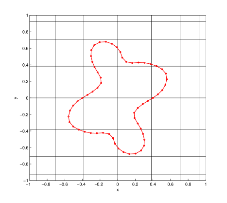
Figure 3: Discretization of the domain $\Omega$ and contour ${\mathcal{C}}$. For clarity, the discretization shown is much coarser than used in the actual computations reported in Section 5.

We let $u_{p;i,j}^{N}\triangleq u_{p}(x_{i},y_{j})$, $i,j=1,\dots,N$ and $\mu_{l}^{M}\triangleq\mu(s_{l})$, $l=1,\dots,M$ denote the discrete nodal values of the unknowns, where $(x_{i},y_{j})$ are the coordinates of the collocation points on the dyadic Chebyshev grid covering $\Omega$, whereas $s_{l}$ are the arc-length coordinates of the points discretizing contour ${\mathcal{C}}$ in Problem P1, i.e., $s_{l}\triangleq(l-1)\frac{L}{M}$, $l=1,\dots,M$. We then construct the vectors ${\bf U}$ and ${\mathbf{m}}$

$$[{\bf U}]_{(i-1)N+j} =u_{p;i,j}^{N}, i,j=1,\dots,N,$$ (27a)

$$[{\mathbf{m}}]_{l} =\mu_{l}^{M}, l=1,\dots,M,$$ (27b)

and will use the symbol $\boldsymbol{\Delta}^{N}$ to denote the discretization of the Laplace operator $\Delta$ based on the Chebyshev spectral collocation approach [56] and corresponding to the Neumann boundary conditions. Thus, discretization of (26a) takes the algebraic form

$$\boldsymbol{\Delta}^{N}{\bf U}={\mathbf{f}}+{\mathbf{q}},$$ (28)

where ${\mathbf{q}}\in{\mathbb{R}}^{N^{2}}$ contains the values of the right-hand side (RHS) function $q$ evaluated at the interior collocation points (and zeros in the entries corresponding to the boundary nodes) and ${\mathbf{f}}\in{\mathbb{R}}^{N^{2}}$ is a vector containing the values of ${\partial u_{h}\over\partial n}$ at the boundary nodes, cf. (26c). It can be expressed as

$${\mathbf{f}}={\bf B}\,{\mathbf{m}},$$ (29)

in which ${\bf B}$ is a $N^{2}\times M$ matrix operator representing the discretization via the trapezoidal rule of the relation

$${\partial u_{h}\over\partial n}\bigg{|}_{{\mathbf{b}}_{i}}=-\frac{1}{2\pi}\oint_{S}\frac{({\mathbf{b}}_{i}-{\mathbf{x}}_{{\mathcal{C}}})\cdot\,{\mathbf{n}}}{|{\mathbf{b}}_{i}-{\mathbf{x}}_{{\mathcal{C}}}|^{2}}\mu({\mathbf{x}}_{{\mathcal{C}}})\,ds,\quad i=1,\dots,4N-4,$$ (30)

where ${\mathbf{b}}_{i}\in\partial\Omega$ (the rows of ${\bf B}$ corresponding to the interior grid points are zero). As regards integral equation (26b), we observe that the logarithmic kernel it contains is in fact singular and, assuming the potential density is a Lipschitz-continuous function of $s$, the integral is defined as an improper one. As a standard approach to deal with this issue [54, 55], we rewrite the kernel as

$$\ln|{\mathbf{x}}_{\mathcal{C}}(t)-{\mathbf{x}}_{\mathcal{C}}(t^{\prime})|=\frac{1}{2}\ln\left\{\frac{|{\mathbf{x}}_{\mathcal{C}}(t)-{\mathbf{x}}_{\mathcal{C}}(t^{\prime})|^{2}}{4\sin^{2}\frac{t-t^{\prime}}{2}}\right\}+\frac{1}{2}\ln\,\left(4\sin^{2}\frac{t-t^{\prime}}{2}\right),$$ (31)

where $t,t^{\prime}\in[0,2\pi]$ are the variables parameterizing contour ${\mathcal{C}}$. Therefore, rewriting the line integral in (26b) as a definite integral, the boundary integral equation becomes

$$\begin{split}-\mu({\mathbf{x}}_{{\mathcal{C}}}(t))&+\overset{(\@slowromancap i@)}{\overbrace{\frac{\gamma}{2\pi\,k}\int_{0}^{2\pi}\mu({\mathbf{x}}_{{\mathcal{C}}}(t^{\prime}))\ln\Bigg{|}\frac{{\mathbf{x}}_{\mathcal{C}}(t)-{\mathbf{x}}_{\mathcal{C}}(t^{\prime})}{2\sin(\frac{t-t^{\prime}}{2})}\Bigg{|}\,r(t^{\prime})\,dt^{\prime}}}\\ &+\overset{(\@slowromancap ii@)}{\overbrace{\frac{\gamma}{4\pi\,k}\int_{0}^{2\pi}\mu({\mathbf{x}}_{{\mathcal{C}}}(t^{\prime}))\ln\Bigg{[}4\sin^{2}\left(\frac{t-t^{\prime}}{2}\right)\Bigg{]}\,r(t^{\prime})\,dt^{\prime}}}=\frac{\gamma}{k}[u_{p}({\mathbf{x}}_{\mathcal{C}}(t))-u_{0}],\quad t\in[0,2\pi]\end{split}$$ (32)

where, assuming that the contour parameterization is uniform in the arc length $s$, we have $r(t)=\big{|}\frac{d{\mathbf{x}}(t)}{dt}\big{|}=\frac{L}{2\pi}$. We note that integral $(\@slowromancap i@)$ has now a regular kernel (with a removable singularity to be more precise) and can be evaluated with spectral accuracy in a straightforward manner using the trapezoidal quadrature. The singularity is now contained in the improper integral $(\@slowromancap ii@)$ which can be evaluated analytically as follows. We approximate the potential density $\mu(t)$ using the spectrally-accurate trigonometric interpolation [55]

$$\mu(t)\approx\sum_{j=1}^{M}\mu^{M}_{j}\,{\mathcal{L}}_{j}(t),$$ (33)

in which ${\mathcal{L}}_{j}(t)$, $j=1,\dots,M$, are the trigonometric cardinal functions

$${\mathcal{L}}_{j}(t)\triangleq\frac{1}{M}\sin\left(\frac{M(t-t_{j})}{2}\right)\,\cot\left(\frac{t-t_{j}}{2}\right),\quad t\in[0,2\pi],\ t\neq\,t_{j},\ j=1,\dots,M,$$

where $t_{j}\triangleq(j-1)\frac{2\pi}{M}$. Defining now

$$R_{j}^{M}(t)\triangleq-\frac{2}{M}\left\{\sum_{m=1}^{M/2-1}\frac{1}{m}\cos\left[\,m(t-t_{j})\right]+\frac{1}{M}\cos\left[\frac{M(t-t_{j})}{2}\right]\right\},\quad j=1,\dots,M,$$ (34)

the improper integral $(\@slowromancap ii@)$ in (32) is approximated as

$$\frac{\gamma}{4\pi\,k}\int_{0}^{2\pi}\mu(t^{\prime})\ln\left[4\sin^{2}\left(\frac{t-t^{\prime}}{2}\right)\right]\,r(t^{\prime})\,dt^{\prime}\approx\frac{\gamma\,L}{4\pi\,k}\sum_{j=1}^{M}\mu^{M}_{j}R_{j}^{M}(t),\ t\in[0,2\pi].$$ (35)

Therefore, collocating integral equation (32) on the grid points $t_{1},\dots,t_{M}$ yields the following discrete problem

$$\left(\mathbf{I}+\frac{\gamma}{k}\mathbf{K}_{1}+\frac{\gamma}{k}\mathbf{K}_{2}\right){\mathbf{m}}+\frac{\gamma}{k}{\bf P}{\bf U}=\frac{\gamma}{k}\,u_{0}\mathbf{1},$$ (36)

where $\mathbf{1}$ is a column vector of dimension $M$ with all entries equal to one and the matrices ${\bf K}_{1}$ and ${\bf K}_{2}$ are defined as, cf. (35),

$$[\mathbf{K}_{1}]_{ij}=-\frac{L}{2\pi\,M}\ln\Biggl{|}\frac{{\mathbf{x}}_{{\mathcal{C}}}(t_{i})-{\mathbf{x}}_{{\mathcal{C}}}(t_{j})}{2\sin\left(\frac{t_{i}-t_{j}}{2}\right)}\Biggr{|},\quad[\mathbf{K}_{2}]_{ij}=\frac{L}{4\pi}\,R_{j}^{M}(t_{i}),\qquad i,j=1,\dots,M,$$ (37)

whereas ${\bf P}$ is an $M\times N^{2}$ matrix representing interpolation of the field $u_{p}$ from the Chebyshev grid onto the points $\{{\mathbf{x}}_{{\mathcal{C}}}(t_{1}),\dots,{\mathbf{x}}_{{\mathcal{C}}}(t_{M})\}$ discretizing the contour ${\mathcal{C}}$. Thus, combining (28) and (36), the final discrete form of system (26) is

$$\begin{bmatrix}-\boldsymbol{\Delta}^{N}\hfil&\mathbf{B}\\ \frac{\gamma}{k}\mathbf{P}\hfil&\mathbf{I}+\frac{\gamma}{k}\mathbf{K}_{1}+\frac{\gamma}{k}\mathbf{K}_{2}\end{bmatrix}\begin{bmatrix}{\bf U}\\ {\mathbf{m}}\end{bmatrix}=\frac{1}{k}\,\begin{bmatrix}{\mathbf{q}}\\ \gamma\,u_{0}\,\mathbf{1}\end{bmatrix}.$$ (38)

The accuracy of approximation represented by system (38) is ultimately determined by the accuracy of the interpolation operator ${\bf P}$, and in principle can be spectral, although for reasons of the numerical stability we have used spline interpolation in the present study. System (38) is readily solved using standard methods of numerical linear algebra, and we refer the reader to thesis [48] for numerical validation and tests of accuracy. Discretization of adjoint system (18) leads to a discrete problem with the same matrix as in (38), but with a different right-hand side. The $L_{2}$ gradient $\boldsymbol{\nabla}^{L_{2}}{\mathcal{J}}$ is obtained from the solution $\left[({\bf U}^{*})^{T}\ ({\mathbf{m}}^{*})^{T}\right]^{T}$ of the discrete adjoint problem using relation (20), where the different terms are computed using boundary conditions (18c)–(18d) and the following identities, known from the potential theory [54, 55],

$${\partial u^{*}_{h}\over\partial n}\bigg{|}_{1}-{\partial u^{*}_{h}\over\partial n}\bigg{|}_{2} =\mu^{*},$$ (39a)

$$\frac{1}{2}\left[{\partial u^{*}_{h}\over\partial n}\bigg{|}_{1}+{\partial u^{*}_{h}\over\partial n}\bigg{|}_{2}\right] =-\frac{1}{2\pi}\oint_{{\mathcal{C}}}\frac{\big{\langle}{\mathbf{n}}({\mathbf{x}}_{\mathcal{C}}),{\mathbf{x}}_{\mathcal{C}}-{\mathbf{x}}^{\prime}\big{\rangle}}{|{\mathbf{x}}_{\mathcal{C}}-{\mathbf{x}}^{\prime}|^{2}}\mu^{*}({\mathbf{x}}^{\prime})\,ds,$$ (39b)

valid for all points ${\mathbf{x}}_{\mathcal{C}}\in{\mathcal{C}}$, where $\langle\cdot,\cdot\rangle$ denotes the inner product in ${\mathbb{R}}^{2}$, $u^{*}=u^{*}_{p}+u^{*}_{h}$ and $\mu^{*}$ is the single-layer potential density associated with $u^{*}_{h}$. We add that the kernel of the integral on the RHS in (39b) is in fact bounded, as we have $\forall_{{\mathbf{x}}^{\prime}\in{\mathcal{C}}}$ $\lim_{{\mathbf{x}}^{\prime}\to{\mathbf{x}}_{{\mathcal{C}}}}\frac{\langle{\mathbf{n}}({\mathbf{x}}_{\mathcal{C}}),{\mathbf{x}}_{\mathcal{C}}-{\mathbf{x}}^{\prime}\rangle}{|{\mathbf{x}}_{\mathcal{C}}-{\mathbf{x}}^{\prime}|^{2}}=\frac{\kappa({\mathbf{x}}_{\mathcal{C}})}{2}$ [54]. Accuracy of the cost functional gradients computed in this way is assessed in the next Section. Finally, we remark that after each step of gradient algorithm (14), the points ${\mathbf{x}}_{{\mathcal{C}}}(t_{i})$, $i=1,\dots,M$, are no longer distributed uniformly in the arc length $s$. In order to retain the spectral accuracy of the solution of equation (32), at every iteration we therefore construct, using spectral Fourier interpolation [56], a new set of collocation points $\{{\mathbf{x}}_{{\mathcal{C}}}(t_{1}),\dots,{\mathbf{x}}_{{\mathcal{C}}}(t_{M})\}$ which are equispaced in the arc-length coordinate. The main modification required to adapt the method described above to Problem P2 concerns the solution of boundary-integral equation (26b). Since the integration domain is no longer periodic, identity (31) must be replaced with a different one and contour ${\mathcal{C}}$ must be discretized using a different set of points [52]. Moreover, the trapezoidal quadratures need to be replaced with the Clenshaw-Curtis quadratures whereas the trigonometric interpolation with a suitable polynomial technique.

5 Computational Results

In this Section we first perform tests to thoroughly validate the computational algorithm introduced in Section 4 for the evaluation of cost functional gradients $\boldsymbol{\nabla}{\mathcal{J}}$. We do this here for Problem P1 and refer the reader to [52] for the corresponding validation tests for Problem P2. Next, we apply this method in the framework of Algorithm 1 to perform shape optimization in a number of test cases concerning Problems P1 and P2. Throughout this Section we take the domain to be $\Omega=[-1,1]\times[-1,1]$.

5.1 Validation of Gradients

A standard computational test employed to ascertain the accuracy of the cost functional gradients in PDE optimization problems is to calculate the Gâteaux differential ${\mathcal{J}}^{\prime}({\mathcal{C}};\zeta{\mathbf{n}})$ for a given contour ${\mathcal{C}}$ and its perturbations $\zeta$ in two different ways: using an approximate finite-difference formula and Riesz identity (16) [57]. Thus, the ratio of these two expressions, denoted

$$\kappa(\varepsilon)\triangleq\frac{{\mathcal{J}}({\mathcal{C}}(\epsilon))-{\mathcal{J}}({\mathcal{C}}(0))}{\epsilon\,\big{\langle}\boldsymbol{\nabla}^{L_{2}}{\mathcal{J}}({\mathcal{C}}(0),\zeta\big{\rangle}_{L_{2}(0,L)}},$$ (40)

should be approximately equal to unity for a range of values of $\epsilon$. Plotting $|\kappa(\epsilon)-1|$ using the logarithmic scale allows one to see the number of significant digits of accuracy captured in the computation. We remark that, since different Riesz representations ($L_{2}$ vs. $H^{1}$) give the same differential ${\mathcal{J}}^{\prime}({\mathcal{C}};\zeta{\mathbf{n}})$, for simplicity in (40) we can use the $L_{2}$ inner product together with the corresponding gradient. To focus attention, we present our validation results for the functional ${\mathcal{J}}({\mathcal{C}})$, i.e., without the length constraint, as the gradient of the latter part does not involve the adjoint variable $u^{*}$. We analyze two sets of results: one in which we fix the contour ${\mathcal{C}}$ and consider different perturbations $\zeta$ and vice versa. For every pair of the contour and the perturbation we study the effect of different resolutions $N$ and $M$. Details concerning the two test cases are collected in Table 2, where the different contours are specified in Table 2, whereas the perturbations tested are given by

$$\zeta_{j}(t)=\sin(j\,t),\quad t=[0,2\pi],\ j=1,2,3,4.$$ (41)

In both validation tests we assume that ${\mathcal{A}}=\Omega$ and use the following distribution of the heat sources and the target temperature profile

$$q(x,y) =50-15x^{2}-15(y-0.5)^{2},$$ (42)

$${\overline{u}}(x,y) =15+\sin(4x-1)\cos(4y-1),$$ (43)

where $-1\leq x,y\leq 1$. The results of TEST #1 and TEST #2 are shown in Figures 5 and 5, respectively. In both cases we note that $\kappa(\epsilon)$ is fairly close to the unity for values of $\epsilon$ spanning several orders of magnitude. The quantity $\kappa(\epsilon)$ deviates from the unity for very small values of $\epsilon$ which is due to the subtractive cancellation (round-off) errors, and for large values of $\epsilon$ which is due to the truncation errors, both of which are well-known effects [58]. Since we use the “differentiate-then-discretize” formulation, one should not expect $|\kappa(\epsilon)-1|$ to be at the level of the machine precision, although this quantity approaches zero as the resolution is refined. We also tested cases in which ${\mathcal{A}}\neq\Omega$ and the length constraint was included obtaining similar results as in Figures 5 and 5. Having thus validated the cost functional gradients, we now move on to discuss solution of the actual optimization problems.

Table 1: Settings for the validation tests of the cost functional gradient $\boldsymbol{\nabla}{\mathcal{J}}$ (Problem P1). The contours and perturbations used are defined in Table 2 and equation (41), respectively.

TEST	Contour ${\mathcal{C}}$	Perturbations $\zeta$	Resolution $(N,~{}M)$	Target Domain ${\mathcal{A}}$
$\#1$	${\mathcal{C}}_{1}$	$\zeta_{1}$, $\zeta_{2}$, $\zeta_{3}$, $\zeta_{4}$	$(50,50)$, $(100,100)$, $(80,300)$	$\Omega$
$\#2$	${\mathcal{C}}_{2}$, ${\mathcal{C}}_{3}$, ${\mathcal{C}}_{4}$, ${\mathcal{C}}_{5}$	$\zeta_{1}$	$(50,50)$, $(80,100)$, $(80,200)$, $(80,300)$, $(80,400)$	$\Omega$

Table 2: Definitions of contours ${\mathcal{C}}_{1},\dots,{\mathcal{C}}_{7}$ used in the different cases studied in Section 5.

Contour	Parametrization $(0\leq t\leq 2\pi)$	Plot
${\mathcal{C}}_{1}$	$x(t)=0.4\cos(t)+0.1$, $y(t)=0.4\sin(t)-0.1$
${\mathcal{C}}_{2}$	$x(t)=0.2\cos(t)+0.4$, $y(t)=0.2\sin(t)+0.4$
${\mathcal{C}}_{3}$	$x(t)=0.3\cos(t)$, $y(t)=0.2\sin(t)$
${\mathcal{C}}_{4}$	$x(t)=0.4(1+0.1\cos(3t))\cos(t)+0.1$, $y(t)=0.4(1+0.1\cos(3t))\sin(t)+0.1$
${\mathcal{C}}_{5}$	$x(t)=0.4(1+0.1\cos(4t))\cos(t)+0.1$, $y(t)=0.4(1+0.1\cos(4t))\sin(t)+0.1$
${\mathcal{C}}_{6}$	$x(t)=\frac{3}{2\pi}\cos(t)-0.4$, $y(t)=\frac{3}{2\pi}\sin(t)+0.3$
${\mathcal{C}}_{7}$	$x(t)=\frac{t-\pi}{\pi}$, $y(t)=0.78$

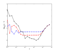
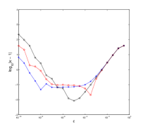
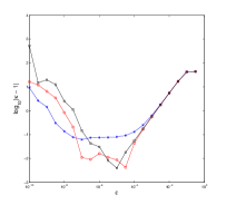
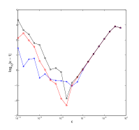
Figure 4: TEST #1 (Table 2): Dependence of $\log_{10}|\kappa(\epsilon)-1|$ on the step size $\epsilon$ in (40) for different perturbations (a) $\zeta_{1}$, (b) $\zeta_{2}$, (c) $\zeta_{3}$ and (d) $\zeta_{4}$, cf. Equation (41), and different resolutions (asterisks) $N=50,\,M=50$, (circles) $N=100,\,M=100$, and (squares) $N=80,\,M=300$.

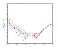
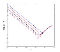
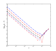
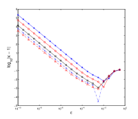
Figure 5: TEST #2 (Table 2): Dependence of $\log_{10}|\kappa(\epsilon)-1|$ on the step size $\epsilon$ in (40) for different contours (a) ${\mathcal{C}}_{2}$, (b) ${\mathcal{C}}_{3}$, (c) ${\mathcal{C}}_{4}$ and (d) ${\mathcal{C}}_{5}$, cf. Table 2, and different resolutions (asterisks) $N=50,\,M=50$, (circles) $N=80,\,M=100$, (squares) $N=80,\,M=200$, (crosses) $N=80,\,M=300$ and (triangles) $N=80,\,M=400$.

5.2 Solution of Optimization Problems

We will study in detail solution of the following three optimization problems with and without the length constraint, as indicated below: in CASE #1 for Problem P1 we examine the convergence of Algorithm 1 without the length constraint for several different initial guesses ${\mathcal{C}}^{(0)}$ for the contour and using ${\mathcal{A}}=\Omega$, in CASE #2 for Problem P1 we consider a configuration in which ${\mathcal{A}}\neq\Omega$ and also study the effect of the length constraint, and in CASE #3 for Problem P2 we investigate a system in which the heat source distribution $q$ corresponds to the temperature field in an actual battery cell, also in the presence of the length constraint. Parameters characterizing the three cases are collected in Table 3. As concerns the heat source distribution $q$, in CASES #1 and #2 it is given by the following expression (Figure 6a)

$$q(x,y)=50-15x^{2}-15\left(y-\frac{1}{2}\right)^{2}\qquad\,(x,y)\in\,\ \Omega,$$ (44)

whereas in CASE #3 it is obtained (by applying the Laplace operator and suitable smoothing) to the temperature distribution determined experimentally in an actual battery cell [59], see Figure 9a. In the different cases the target temperature field is given by the following expressions (see also Figure 6b)

$$\textrm{CASE}\ \#1,2:\quad {\overline{u}}(x,y) =15+\sin(2\pi\,x+\pi)\cos\left(2\pi\,y+\frac{\pi}{2}\right),\quad (x,y)\in\,\ {\mathcal{A}},$$ (45a)

$$\textrm{CASE}\ \#3: {\overline{u}}(x,y) =30 (x,y)\in\,\ \Omega.$$ (45b)

In CASE #1 and #2 the distribution of heat sources (44) and the target temperature field (45a) have been chosen to test the algorithm in the situation when the source field varies slowly, whereas the target field exhibits a significant variability, cf. Figures 6a and 6b. On the other hand, in CASE #3 the constant target temperature field (45b) represents a typical engineering objective. The specific values assumed by the fields $q$ and $\overline{u}$ do not have a physical significance and were selected to make the optimization problem sufficiently challenging. The tolerances in Algorithm 1 are set to $\varepsilon_{{\mathcal{J}}}=10^{-3}$ and $\varepsilon_{\tau}=10^{-8}$.

Table 3: Parameters used in the solution of the three optimization problems in Section 5.2. The contours used as the initial guesses ${\mathcal{C}}^{(0)}$ are defined in Table 2.

CASE	$q$	${\overline{u}}$	$(N,~{}M)$	$\alpha$	$L_{0}$	$\ell$	${\mathcal{C}}^{(0)}$	${\mathcal{A}}$
#1 (P1)	Eq. (44)	Eq. (45a)	(50,100)	0	—	0.1, 0.3	${\mathcal{C}}_{2}$, ${\mathcal{C}}_{3}$, ${\mathcal{C}}_{4}$, ${\mathcal{C}}_{5}$	$\Omega$
#2 (P1)	Eq. (44)	Eq. (45a)	(50,100)	$10^{2}$	3.0	0.1	${\mathcal{C}}_{6}$	$[-0.5,1]\times[-0.5,1]$
#3 (P2)	Fig. 9a	Eq. (45b)	(50,100)	$1,10$, $10^{2},10^{3}$	6.0	0.1,0.25	${\mathcal{C}}_{7}$	$\Omega$

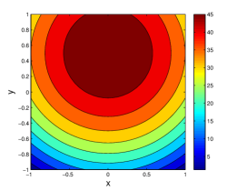
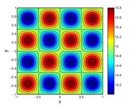
Figure 6: (a) Distribution of heat sources $q$, cf. (44), and (b) target temperature field ${\overline{u}}$, cf. (45a), used in CASE #1 and #2.

       

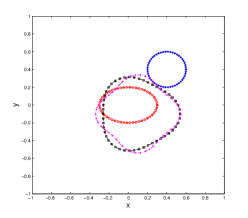
(a) Initial contour shapes ${\mathcal{C}}_{2}$, ${\mathcal{C}}_{3}$, ${\mathcal{C}}_{4}$ and ${\mathcal{C}}_{5}$ (for clarity they are represented using fewer points than used in the actual computations)

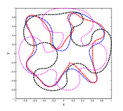
(b) Optimal contour shapes $\tilde{{\mathcal{C}}}$ corresponding to the initial contours shown in Figure (a)

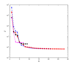
(c) Evolution of functionals ${\mathcal{J}}({\mathcal{C}}^{(n)})$ for iterations starting with the initial contours shown in Figure (a)

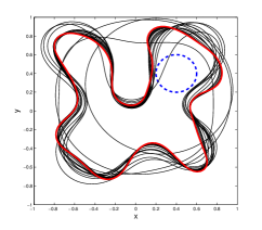
(d) Evolution of contours ${\mathcal{C}}^{(n)}$ with iterations in the problem with initial shape ${\mathcal{C}}_{2}$ (dashed line)

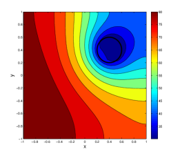
(e) Initial temperature field $u({\mathcal{C}}_{2})$

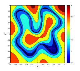
(f) Optimal temperature field $u(\tilde{{\mathcal{C}}})$ in the case with initial contour ${\mathcal{C}}_{2}$

Figure 7: Results illustrating solution of the optimization problems in CASE #1, cf. Table 3, using different initial contours (asterisks) ${\mathcal{C}}_{2}$, (circles) ${\mathcal{C}}_{3}$, (squares) ${\mathcal{C}}_{4}$, (pluses) ${\mathcal{C}}_{5}$, cf. Table 2.

        

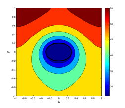
(g) Initial temperature field $u({\mathcal{C}}_{3})$

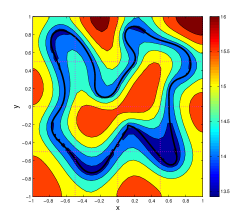
(h) Optimal temperature field $u(\tilde{{\mathcal{C}}})$ in the case with initial contour ${\mathcal{C}}_{3}$

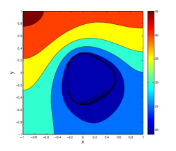
(i) Initial temperature field $u({\mathcal{C}}_{4})$

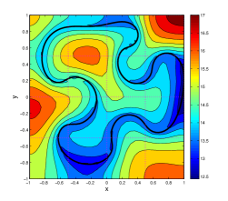
(j) Optimal temperature field $u(\tilde{{\mathcal{C}}})$ in the case with initial contour ${\mathcal{C}}_{4}$

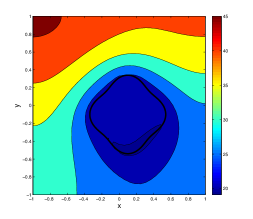
(k) Initial temperature field $u({\mathcal{C}}_{5})$

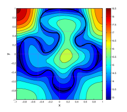
(l) Optimal temperature field $u(\tilde{{\mathcal{C}}})$ in the case with initial contour ${\mathcal{C}}_{5}$

Figure 7: (continued) Results illustrating solution of the optimization problems in CASE #1, cf. Table 3. The grid shown in the Figures in the right column corresponds to the cellular pattern of the target field ${\overline{u}}$, cf. Figure 6(b).

The results characterizing the performance of Algorithm 1 in CASE #1 are collected in Figure 7. First of all, we note that, depending on the choice of the initial guess ${\mathcal{C}}^{(0)}$ for the contour in (14), cf. Figure 7a, the iterations in fact converge to quite distinct locally optimal shapes, cf. Figure 7b, providing evidence for the existence of multiple local minima in the optimization problem, as discussed in Section 3. We also note that the decrease of cost functional ${\mathcal{J}}({\mathcal{C}}^{(n)})$ with iterations $n$ is quite different in these different cases, cf. Figure 7c. In Figure 7d we show the intermediate shapes found at the consecutive iterations of the algorithm starting from the initial guess ${\mathcal{C}}_{2}$ for which the largest decrease was obtained in the cost functional. We observe that “simpler” initial guesses (i.e., a circle or an ellipse) tend to lead to “better” local minimizers. However, the final temperature distributions $u(\tilde{{\mathcal{C}}})$ obtained from the different initial guesses all capture features of the cellular pattern characterizing the target distribution ${\overline{u}}$, see Figures 7f,h,j,l vs. Figure 6b.

     

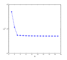
(a) Evolution of cost functional ${\mathcal{J}}_{\alpha}({\mathcal{C}}^{(n)})$ with iterations

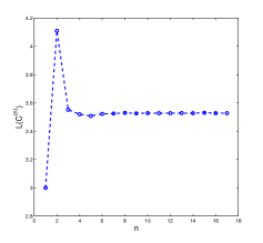
(b) Evolution of contour length $L({\mathcal{C}}^{(n)})$ with iterations

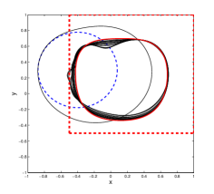
(c) Evolution of contours ${\mathcal{C}}^{(n)}$ with iterations; the initial contour ${\mathcal{C}}_{7}$ is marked with thin dashed line and the optimal shape $\tilde{{\mathcal{C}}}$ appears in red

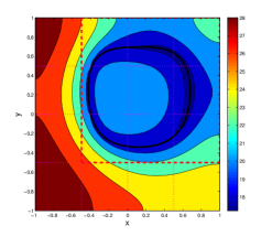
(d) Optimal temperature distribution $u(\tilde{{\mathcal{C}}})$

Figure 8: Results illustrating solution of the optimization problem in CASE #2, cf. Table 3. The rectangles marked with thick dashed lines in Figures (c) and (d) indicate the subregion ${\mathcal{A}}$ where the target temperature ${\overline{u}}$ is specified.

The data illustrating the performance of Algorithm 1 in CASE #2 is shown in Figure 8. Since in this case we include the length constraint with a rather large value of the penalty parameter ($\alpha=10^{2}$), the optimal contours are not allowed to deform much (Figure 8c). However, we remark that the algorithm is able to “shift” the contour so that the optimal shape $\tilde{{\mathcal{C}}}$ is enclosed within the target domain ${\mathcal{A}}$ in which the temperature field ${\overline{u}}$ is defined (Figure 8d).

   

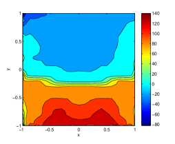
(a) Distribution of heat sources $q$ [59]

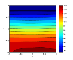
(b) Initial temperature field $u({\mathcal{C}}_{7})$

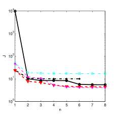
(c) Evolution of cost functional ${\mathcal{J}}({\mathcal{C}}^{(n)})$ with iterations

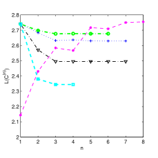
(d) Evolution of contour length $L({\mathcal{C}}^{(n)})$ with iterations

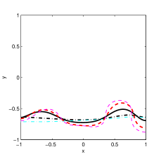
(e) Optimal contours $\tilde{{\mathcal{C}}}$ obtained without the length constraint

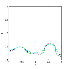
(f) Optimal contours $\tilde{{\mathcal{C}}}$ obtained with the length constraint

Figure 9: Results illustrating solution of the optimization problems in CASE #3, cf. Table 3; in Figures (c) and (e): (solid) $u_{0}=10=\textrm{Const}$, (thick dashed) $T_{a}=10$ and $T_{b}=16$, (thin dashed) $T_{a}=10$ and $T_{b}=19$, (thick dash-dotted) $T_{a}=4$ and $T_{b}=10$, (thin dash-dotted) $T_{a}=1$ and $T_{b}=10$; in Figures (d) and (f): (thin dashed) $\alpha=0$, (thick dash-dotted) $\alpha=1$, (dotted) $\alpha=10$, (thin dash-dotted) $\alpha=10^{2}$, (thick dashed) $\alpha=10^{3}$.

   

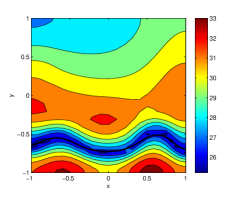
(g) Optimal temperature distribution $u(\tilde{{\mathcal{C}}})$ obtained with $u_{0}=10=\textrm{Const}$ and $\alpha=0$

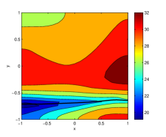
(h) Optimal temperature distribution $u(\tilde{{\mathcal{C}}})$ obtained with $T_{a}=1$, $T_{b}=10$ and $\alpha=0$

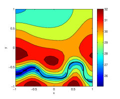
(i) Optimal temperature distribution $u(\tilde{{\mathcal{C}}})$ obtained with $T_{a}=10$, $T_{b}=19$ and $\alpha=0$

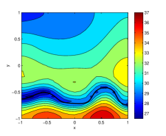
(j) Optimal temperature distribution $u(\tilde{{\mathcal{C}}})$ obtained with $T_{a}=10$, $T_{b}=19$ and $\alpha=1000$

Figure 9: (continued) Results illustrating solution of the optimization problems in CASE #3 with different $u_{0}$, cf. (2).

The data concerning CASE #3 is collected in Figure 9. Using the contour shown in Figure 9b as the initial guess (cf. Table 2), we first solve Problem P2 assuming $u_{0}=\textrm{Const}$ and with the length constraint not enforced ($\alpha=0$). Then, using thus obtained optimal shape (marked with the solid line in Figure 9e) as the initial guess, we solve Problem P2 again, now allowing $u_{0}$ to vary with the arc length $s$. Mimicking changes in the inflow/outflow temperature of the coolant liquid, this is achieved by decreasing $T_{a}$ or increasing $T_{b}$ in (2) and corresponds to, respectively, dash-dotted and dashed contours in Figure 9e. In Figure 9c we observe that in the initial optimization the cost functional drops by over three orders of magnitude during less than 10 iterations (in the subsequent problems which have better initial guesses this decrease is smaller). Finally, we consider the case with $T_{a}=10$ and $T_{b}=19$, and solve the optimization problem with the length constraint using $L_{0}=2.3$ and increasing values of $\alpha$. The resulting optimal contour shapes are shown in Figure 9f, whereas Figure 9d presents the evolution of the contour length $L({\mathcal{C}}^{(n)})$ with iterations for different values of $\alpha$. As expected, we see that for increasing values of $\alpha$ the contour length approaches the prescribed value $L_{0}$ while the contours themselves become less deformed. The temperature fields $u(x,y)$ obtained in the cases with $u_{0}=10=\textrm{Const}$, $T_{a}=1$ and $T_{b}=10$, and $T_{a}=10$ and $T_{b}=19$, cf. (2), and without the length constraint are shown in Figures 9g,h,i. This last case with the length constraint and $\alpha=1000$ is shown in Figure 9j. We see that, as compared to the temperature corresponding to the initial guess for the contour (Figure 9b), the optimal distributions in Figures 9g,h,i,j have the temperature ranges much closer to target field (43). We also observe that, with the exception of the case in which the inflow temperature $T_{a}$ is quite low (Figure 9h), the optimal contour shapes tend to weave around the two hot spots in the heat source distribution (Figure 9a) in a complicated manner.

6 Conclusions and Future Work

In this investigation we have addressed the problem of shape optimization for a system of elliptic PDEs subject to mixed interface boundary conditions which models the steady-state heat transfer in 2D. Our continuous optimization formulation relies on Sobolev shape gradients obtained using the shape-differential calculus and explicit interface tracking employed to represent the optimized contour, all of which are rather well known approaches. The key novel contribution of this work is the method we introduced to numerically evaluate the shape gradients. By splitting the adjoint system into two coupled subproblems we could achieve optimal accuracy for each of the subproblems. In particular, the proposed boundary-integral formulation exploits the analytical (potential) structure of the problem and, as demonstrated by the exhaustive validation tests presented in Section 5.1, offers high numerical accuracy without the need to construct a boundary-fitted mesh at every iteration, as required in other approaches based on explicit interface tracking [15]. As a result, the proposed method is quite efficient from the computational point of view and, as shown in Section 5.2, can deal with fairly complicated contour shapes in an easy and straightforward manner. While boundary-integral formulations have been used to study the shape sensitivities of elliptic PDEs (e.g., [37, 38, 41]), the method we introduced is designed for higher accuracy than previous approaches.

As compared to the “discretize-then-differentiate” approaches, they key advantage of the continuous formulation used here is that, as discussed at the end of Section 4, it offers the freedom to remesh the points discretizing the contour which is crucial to achieving spectral accuracy in the solution of the boundary integral equation. On the contrary, in the discrete setting such remeshing would actually require one to set up a new optimization problem (corresponding to the new set of the discrete control variables). Moreover, it is also not evident how the analytic treatment of singularities described in Section 4 could be employed in the discrete setting. In regard to the level-set-based interface capturing methods, the present approach arguably offers more flexibility in the high-accuracy treatment of the complex interface boundary conditions.

Optimizations performed on three test problems led to rather nonintuitive optimal shapes of the contour which differed significantly from the initial guesses provided based on the “engineering intuition”, reflecting the geometric nonlinearity and nonlocality of the governing system. Smoothness of the contours was enforced by defining the cost functional gradients in a suitable Sobolev space. This, combined with the interpolation technique described at the end of Section 4, allowed for an accurate representation of even strongly deformed contours using a rather modest number of points ($M=100$ in CASES #1, #2, and #3, cf. Table 3). Evidence was also shown for the presence of multiple local minima. In Problem P1, when the length constraint was not imposed, the optimal temperature distributions were found to capture the main features of the target temperature field ${\overline{u}}$. On the other hand, the presence of the length constraint restricted the ability of the algorithm to deform the contour, although it was still capable of “shifting” the contour to a different part of the domain $\Omega$ without significant shape changes. It ought to be added that extension of the proposed approach to three-dimensional (3D) configurations is conceptually straightforward. Aside from the need to work with the 3D fundamental solutions in expressions resulting from ansatz (25), some technical complications may arise from the fact that the boundary integral equations will be formulated on 2D surfaces, rather than on 1D contours which, in particular, may make achieving high numerical accuracy more difficult.

The formulation developed in this study leads to the following open problems of a more fundamental character. Our adjoint system (18) was derived in the PDE setting [47] and only then recast in terms of the boundary-integral formulation for the purpose of the numerical solution. On the other hand, one could begin with the boundary-integral formulation of governing system (3) which, after shape differentiation, would give rise to an integral expression with more singular, possibly hypersingular, kernels. Assessing the relative advantages and disadvantages of such an alternative approach is an interesting open question and is left to the future research (we mention that sensitivity calculations based on hypersingular integral equations have already been discussed in [41]). In addition, our future work will also involve generalizations of the proposed approach to mathematical models of the battery system more complex than (3) and accounting for some effects of the actual flow of the coolant fluid in channels of finite thickness (see Figure 1b). We also intend to explore optimization of the topology of the contours [60].

References

- [1] V. Srinivasan, “Batteries for Vehicular Applications”, in Physics Of Sustainable Energy: Using Energy Efficiently and Producing It Renewably, AIP Conf. Proc. 1044, 283–296, (2008).
- [2] N. A. Chaturvedi, R. Klein, J. Christensen, J. Ahmed, and A. Kojic, “Algorithms for Advanced Batter-Management Systems: Modeling, Estimation, and Control for Lithium-Ion Batteries” IEEE Control Systems Magazine 30, 49–68, (2010).
- [3] M. D. Gunzburger, Perspectives in flow control and optimization, SIAM, Philadelphia, (2003).
- [4] A. Jarrett and I. Y. Kim, “:Design optimization of electric vehicle battery cooling plates for thermal performance”, Journal of Power Sources 196 10359–10368, (2011).
- [5] C. H. Lan, C. H. Cheng and C. Y. Wu, “Shape Design for Heat Conduction Problems using Curvilinear Grid Generation, Conjugate Gradient and Redistribution Methods”, Numerical Heat Transfer, Part A 39, 487–510, (2001).
- [6] C. H. Cheng and M. H. Chang, “A Simplified Conjugate Gradient Method for Shape Identification Based on Thermal data”, Numerical Heat Transfer, Part B 43, 489–507, (2003).
- [7] C. H. Cheng and M. H. Chang, “Shape identification by inverse heat transfer method” Journal of Heat Transfer 125, 224–231, (2003).
- [8] C. H. Cheng and M. H. Chang, “A simplified conjugate gradient method for shape identification based on thermal data”, Numerical Heat Transfer, Part B 43, 487–507, (2003).
- [9] A. Ashrafizadeh, G. D. Raithby, and G. D. Stubley, “Direct design of shape”, Numerical Heat Transfer, Part B 41, 501–520, (2002).
- [10] B. Mohammadi and O. Pironneau, Applied Shape Optimization for Fluids, Oxford University Press, (2009).
- [11] J. Sokolowski and J.-P. Zolésio, Introduction to shape optimization: shape sensitivity analysis, Springer, (1992).
- [12] M. C. Delfour and J.-P. Zolésio, Shape and Geometries — Analysis, Differential Calculus and Optimization, SIAM, (2001).
- [13] J. Haslinger and R. A. E. Mäkinen, Introduction to Shape Optimization: Theory, Approximation, and Computation, SIAM, Philadelphia, (2003).
- [14] S. Schmidt and V. Schulz, “Shape derivatives for general objective functions and the incompressible Navier-Stokes equations”, Control and Cybernetics 39, 677–713, (2010).
- [15] S. W. Walker, and M. J. Shelley, “Shape Optimization of Peristaltic Pumping”, Journal of Computational Physics 229, 1260–1291, (2010).
- [16] G. Z. Yang and N. Zabaras, ”The adjoint method for an inverse design problem in the directional solidification of binary alloys”, Journal of Computational Physics, 140, 432–452, 1998.
- [17] M. Hinze and S. Ziegenbalg, “Optimal control of the free boundary in a two-phase Stefan problem”, Journal of Computational Physics 223, 657–684 (2007).
- [18] O. Volkov and B. Protas, “An inverse model for a free-boundary problem with a contact line: steady case”, Journal of Computational Physics 228, 4893–4910, (2009).
- [19] O. Volkov, B. Protas, W. Liao and D. Glander, “Adjoint-Based Optimization of Thermo-Fluid Phenomena in Welding Processes”, Journal of Engineering Mathematics, 65, 201–220, (2009).
- [20] M. K. Bernauer and R. Herzog, “Optimal Control of the Classical Two-Phase Stefan Problem in level Set Formulation”, SIAM Journal on Scientific Computing 33, 342–363, (2011).
- [21] S. Repke, N. Marheineke and R. Pinnau, “Two adjoint-based optimization approaches for a free surface Stokes flow”, SIAM J. Appl. Math. 71, 2168–2184 (2011).
- [22] S. Osher and R. Fedkiw, “Level Set Methods and Dynamic Implicit Surfaces”, Springer (2002).
- [23] F. Santosa, “A level set approach for inverse problems involving obstacles”, ESAIM: Control, Optimisation and Calculus of Variations 1 17–33, (1996).
- [24] Z. Li and K. Ito, The Immersed Interface Method: Numerical Solutions of PDEs Involving Interfaces and Irregular Domains, SIAM, (2006).
- [25] K. Ito, K. Kunisch, and Z. Li, “Level-set function approach to an inverse interface problem”, Inverse Problems 17, 1225–1242, (2001).
- [26] K. Ito, “Level set methods for variational problems and applications”, Control and Estimation of Distributed Parameter Systems 143, 203–217, (2003).
- [27] F. Chantalat, Ch.-H. Bruneau, C. Galusinski and A. Iollo, “Level-set, penalization and Cartesian meshes: A paradigm for inverse problems and optimal design”, Journal of Computational Physics 228, 6291–6315, (2009).
- [28] M. Burger, “A level set method for inverse problems”, Inverse Problems 17, 1327–1355, (2001).
- [29] M. Burger, “A framework for the construction of level set methods for shape optimization and reconstruction”, Interfaces and Free Boundaries 5, 301–329, (2003).
- [30] G. Doǧan, P. Morin, R. H. Nochetto, and M. Verani, “Discrete gradient flows for shape optimization and applications”, Computer Methods in Applied Mechanics and Engineering 196, 3898–3914, (2007)
- [31] G. Sundaramoorthi, A. Yezzi, and A. C. Mennucci, “Sobolev active contours”, International Journal of Computer Vision 73, 345–366, (2007)..
- [32] P. Kazemi and I. Danaila, “Sobolev gradients and image interpolation”, SIAM Journal on Imaging Sciences (to appear), (2012).
- [33] C. H. Huang and B. H. Chao, “An inverse geometry problem in identifying irregular boundary configurations”, International Journal of Heat and Mass Transfer 40, 2045–2053, (1997). .
- [34] C. H. Huang and T. Y. Hsiung, “An inverse design problem of estimating optimal shape of cooling passages in turbine blades”, International Journal of Heat and Mass Transfer, 42, 4307–4319, (1999).
- [35] C. H. Huang and C. C. Shih, “A shape identification problem in estimating simultaneously two interfacial configurations in a multiple region domain”, Applied Thermal Engineering 26, 77–88, (2006).
- [36] C. H. Huang and C. Y. Liu, “A three-dimensional inverse geometry problem in estimating simultaneously two interfacial configurations in a composite domain”, International Journal of Heat and Mass Transfer 53, 48–57, (2010).
- [37] A. Novruzi and J. R. Roche, Newton’s Method In Shape Optimisation: A Three-Dimensional Case, BIT 40, 102–120, (2000).
- [38] A. Henrot and G. Villemin, “An Optimum Design Problem In Magnetostatics”, Mathematical Modelling and Numerical Analysis 36, 223–239, (2002).
- [39] A. Abba, S. Fausto and C. D’Angelo, “A 3D Shape Optimization Problem in Heat Transfer: Analysis and Approximation via BEM”, Mathematical Models and Methods in Applied Sciences 16, 1243–1270, (2006).
- [40] H. Harbrecht and J. Tausch, “On The Numerical Solution Of A Shape Optimization Problem For The Heat Equation”, SIAM J. Sci. Comput. 35, A104–A121, (2013).
- [41] G. Rus and R. Gallego, “Hypersingular shape sensitivity boundary integral equation for crack identification under harmonic elastodynamic excitation”, Comput. Methods Appl. Mech. Engrg. 196, 2596–2618, (2007).
- [42] P. Grisvard, Elliptic Problems in Nonsmooth Domains, SIAM, (2011).
- [43] M. E. Gurtin. Thermomechanics of Evolving Phase Boundaries in the Plane, Oxford University Press, (1993).
- [44] W. H. Press, B. P. Flanner, S. A. Teukolsky and W. T. Vetterling, Numerical Recipes: the Art of Scientific Computations, Cambridge University Press, Cambridge, (1986).
- [45] J. Nocedal and S. J. Wright, Numerical Optimization, Springer, (2000).
- [46] M. S. Berger, Nonlinearity and Functional Analysis, Academic Press, (1977).
- [47] B. Protas, Remarks on Symbolic Generation of Adjoint Systems in PDE Optimization Problems, submitted, (2011).
-
[48]
X. Peng, Optimal Geometry in a Simple Model of
Two-Dimensional Heat Transfer, Master’s Thesis, McMaster
University available at
http://digitalcommons.mcmaster.ca/opendissertations/5212, (2011). - [49] B. Protas, T. Bewley and G. Hagen, “A computational framework for the regularization of adjoint analysis in multiscale PDE systems”, Journal of Computational Physics 195, 49–89, (2004).
- [50] J. W. Neuberger, Sobolev Gradients and Differential Equations, Springer, (2010).
- [51] I. Danaila and P. Kazemi, “A new Sobolev gradient method for direct minimization of the Gross-Pitaevskii energy with rotation”, SIAM Journal on Scientific Computing 32, 2447–2467, (2010).
- [52] K. Niakhai, Shape Optimization of Elliptic PDE Problems on Complex Domains, Master’s Thesis, McMaster University (in preparation), (2013).
- [53] Y. Li and A. T. Layton, “Accurate computation of Stokes flow driven by an open immersed interface”, Journal of Computational Physics 231, 5195–5215, (2012).
- [54] W. Hackbusch, Integral Equations: Theory and Numerical Treatment, Birkhäuser, (1995).
- [55] R. Kress, Linear Integral Equations, Springer, (1999).
- [56] L. N. Trefethen, Spectral Methods in Matlab, SIAM, (2000).
- [57] C. Homescu, I. M. Navon and Z. Li, “Suppression of vortex shedding for flow around a circular cylinder using optimal control”, Int. J. Numer. Meth. Fluids 38, 43–69, (2002).
- [58] B. Protas and W. Liao, “Adjoint-Based Optimization of PDEs in Moving Domains”, J. Comp. Phys. 227, 2707–2723, (2008).
- [59] U. S. Kim, C. B. Shin and C. S. Kim, “Modeling for the scale-up of a lithium-ion polymer battery” Journal of Power Sources 189, 841–846, (2009).
- [60] J. Sokołowski and A. Żochowski, “On The Topological Derivative In Shape Optimization”, SIAM J. Control Optim. 37, 1251–1272, (1999).