A Critical Examination on L/E Analysis in the Underground Detectors with a Computer Numerical Experiment Part 1

Abstract

There are many uncertain factors involved in the cosmic ray experiments (on atmospheric neutrinos) which seek to confirm the existence of neutrino oscillations with definite oscillation parameters. For the purpose, it is desirable to select those physical events in which uncertain factors are involved to a minimum extent and to examine them in a rigorous manner. In the present paper we consider neutrino events due to quasi-elastic scattering (QEL) as the most reliable events among various candidate events to be analyzed, and have carried out the first step of an $L/E$ analysis which aims to confirm the survival probability with a Numerical Computer Experiment. The most important factor in the survival probability is $L_{\nu}/E_{\nu}$, but this cannot be measured for such neutral particles. Instead, $L_{\mu}/E_{\mu}$ is utilized in the $L/E$ analysis, where $L_{\nu}$, $L_{\mu}$, $E_{\nu}$ and $E_{\mu}$ denote the flight path lengths of the incident neutrinos, those of the emitted leptons, the energies of the incident neutrinos and those of the emitted leptons, respectively. According to our Computer Numerical Experiment, the relation of $L_{\nu}/E_{\nu}\approx L_{\mu}/E_{\mu}$ doesn’t hold. In subsequent papers, we show the results on an $L/E$ analysis with the Computer Numerical Experiment based on our results obtained in the present paper.
PACS: 13.15.+g, 14.60.-z

1 Introduction

In the detection of neutrino oscillation of the atmospheric neutrinos by underground detectors, one examines the zenith angle distribution of the neutrino events, utilizing the different flight path lengths of neutrinos due to the morphology of the Earth, based on the survival probability for neutrinos of given flavor. For example, for $\nu_{\mu}\rightarrow\nu_{\mu}$ , it is given as,

$$P(\nu_{\mu}\rightarrow\nu_{\mu})=1-sin^{2}2\theta\cdot sin^{2}(1.27\Delta m^{2}L_{\nu}/E_{\nu}),$$ (1)

where $\theta$ is the mixing angle between the mass eigenstate and the weak eigenstate and $\Delta m^{2}$ is the difference of the squared mass eigenvalues[1]. The quantities $L_{\nu}$ and $E_{\nu}$ denote the flight length of the neutrino from the starting point above the Earth to the generation of the neutrino event concerned and the neutrino energy, respectively.

The analysis of the zenith angle distribution of the neutrino events of the atmospheric neutrinos should be recognized as a test of an indirect proof of the survival probability of a given flavor of neutrino oscillation, while the $L/E$ analysis aims at a direct proof of the survival probability itself. In this sense, confirmation of the first maximum of oscillation in the survival probability through the $L/E$ analysis should be carefully examined in a rigorous manner, because the confirmation should be regarded as the ultimate proof of the existence of the neutrino oscillation probability.

In the $L/E$ analysis, one tries to observe this survival probability directly, through the observation of the first, second and third maxima in the oscillations, where $P(\nu_{\mu}\rightarrow\nu_{\mu})$ have the minimum values. There are many candidates of neutrino events for $L/E$ analysis. In underground detectors, one can observe different kinds of neutrino events, such as Sub-GeV e-like, Multi-GeV e-like, Sub-GeV $\mu$-like, Multi GeV $\mu$-like, Multi-ring Sub-GeV $\mu$-like, Multi-Ring Multi-GeV $\mu$-like, Upward Stopping Muon events and Upward Through Going Muon Events and so on, resulting from the morphology or the nature of the physical interaction - elastic scattering off an electron, quasi elastic scattering off a nucleon, single meson production, deep inelastic scattering, coherent pion production and so on[1].

Considering that there are many uncertain factors in the study of neutrino oscillations with the use of the cosmic ray beam (atmospheric neutrinos), one should carry out the neutrino oscillation study with the neutrino events of least ambiguity among the possible candidates to be analyzed. Thus, it is reasonable to select those quasi-elastic scattering (QEL) events classified as Fully Contained Events, where the generation points of the interaction as well as their termination points remain inside the detector. In addition to its simple shape, from the nature of the physical interaction and also from the viewpoint of the morphology, the directions of the emitted leptons and their energy can be determined more reliably than in the case of any other candidates.

2 The characteristics of the computer numerical experiment

In the present paper, we carry out the first step of $L/E$ analysis of the neutrino events which are only due to quasi elastic scattering (QEL), such as $\nu+N\rightarrow N+lepton$, and are confined fully inside the detectors (Fully Contained Events) with a Computer Numerical Experiment. In addition to their high quality, their frequency is also highest among all possible events and, consequently, statistics of the events for the purpose of extracting definite conclusions about neutrino oscillation are not a worry. One does not have to rely on other experimental data, based on insufficient information, to increase statistics. In our Computer Numerical Experiment, we ”construct” virtually the underground detector in the computer and sample randomly a neutrino energy from the energy spectrum of incident neutrinos on the Earth, follow the neutrino events giving rise to QEL, considering the interior structure of the Earth, ”measure” both the directions and the energies of the emitted leptons (electrons and muons) in the QEL events and finally confirm whether these events are really confined inside the detector or escape from it by following the emitted leptons in a stochastic manner. In other words, we reproduce the neutrino events due to atmospheric neutrino inside the computer. In this sense we obtain pseudo experimental data, in contrast to the real experimental data in the underground detectors. As we adopt the same initial or boundary conditions which is applied to the real underground detectors, such as detector geometry[1], live days for the experiment[1], incident neutrino energy spectrum[2] and the interior structure of the Earth[3], we can say that our pseudo experimental data are directly comparable with the corresponding real experimental data, allowing for the uncertainties occurring in the real experiments.

Due to the characteristics of the Computer Numerical Experiment, the pseudo experimental data thus obtained have no ”experimental errors”. However, even if the phenomena concerned may be proved to be realized with the Computer Numerical Experiment, these phenomena are not always detected in the real experiments. They may be detected in some case, maybe not in another, depending on the constraints of the real detectors concerned. Thus, careful and detailed examination of the analysis of neutrino events due to QEL which are fully contained in the detector are essentially important for the sake of the examination of the most reliable $L/E$ analysis.

Verification of the existence of neutrino oscillations through $L/E$ analysis, if they exist, means confirming the existence of the maximum oscillation where $P(\nu_{\mu}\rightarrow\nu_{\mu})$ have minimum values. It should be noticed that the arguments $L_{\nu}$ and $E_{\nu}$ contained in the survival probability cannot be measured for neutral particles and instead, $L_{\mu}$ and $E_{\mu}$ are utilized as estimators of $L_{\nu}$ and $E_{\nu}$, where $L_{\nu}$ is the flight path length of the produced lepton and $E_{\nu}$ is its energy.

Therefore, in the study on the detection of the survival probability it is implicitly assumed that the following equation holds.

$$L_{\nu}/E_{\nu}\approx L_{\mu}/E_{\mu}$$ (2)

In the present paper, we focus our attention on the examination of the validity of Eq.(2) through the analysis of the Fully Contained Events among QEL events with the Computer Numerical Experiment.

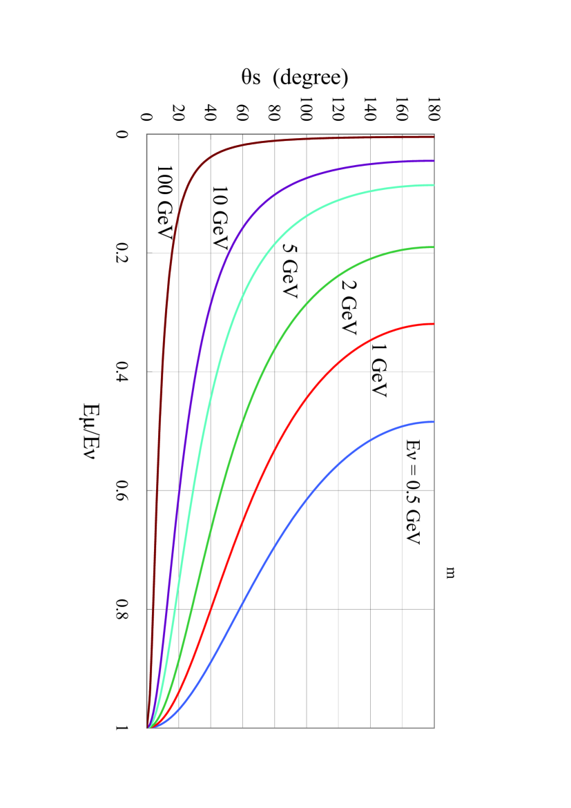
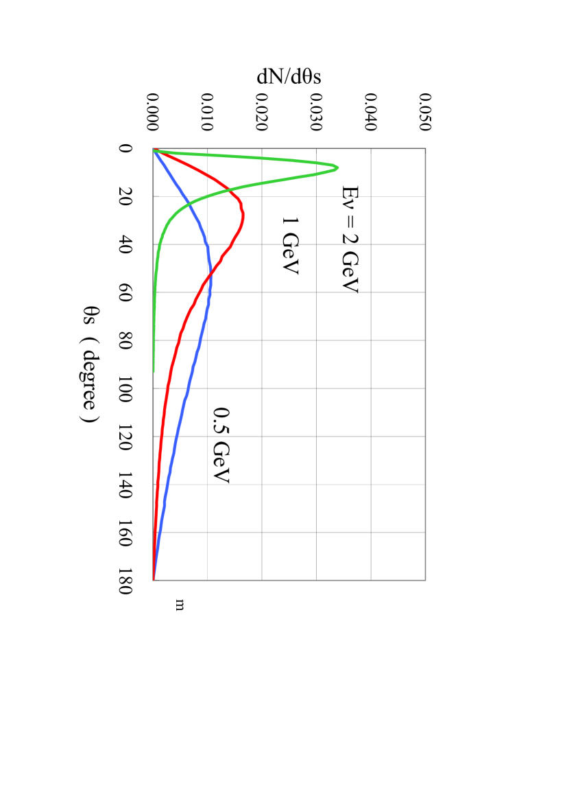
Figure 1: The relation between the energy of the muon and its production angle for different incident muon neutrino energies, 0.5, 1, 2, 5, 10 and 100 GeV.

Figure 2: The distribution functions of the scattering. The angles of the muon for muon-neutrino with incident energies, 0.5 , 1.0 and 2 GeV. Each curve is obtained by the Monte Carlo method (one million sampling per curve).

3 Neutrino events due to quasi-elastic scattering which are fully contained in the detector

3.1 Differential cross section for quasi-elastic scattering and spreads of the scattering angles

Here we obtain the distribution functions for the scattering angles of the produced leptons. We examine the following quasi elastic scattering (QEL) events:

$$\nu_{e}+n\longrightarrow p+e^{-}$$

$$\nu_{\mu}+n\longrightarrow p+\mu^{-}$$

$$\bar{\nu}_{e}+p\longrightarrow n+e^{+}$$ (3)

$$\bar{\nu}_{\mu}+p\longrightarrow n+\mu^{+},$$

The differential cross section for QEL is given as follows[4].

$$\frac{{\rm d}\sigma_{\ell(\bar{\ell})}(E_{\nu(\bar{\nu})})}{{\rm d}Q^{2}}=$$

$$\frac{G_{F}^{2}{\rm cos}^{2}\theta_{C}}{8\pi E_{\nu(\bar{\nu})}^{2}}\Biggl{\{}A(Q^{2})\pm B(Q^{2})\biggl{[}\frac{s-u}{M^{2}}\biggr{]}$$

$$+C(Q^{2})\biggl{[}\frac{s-u}{M^{2}}\biggr{]}^{2}\Biggr{\}},$$ (4)

where

$$A(Q^{2}) = \frac{Q^{2}}{4}\Biggl{[}f^{2}_{1}\biggl{(}\frac{Q^{2}}{M^{2}}-4\biggr{)}+f_{1}f_{2}\frac{4Q^{2}}{M^{2}}$$

$$+f_{2}^{2}\biggl{(}\frac{Q^{2}}{M^{2}}-\frac{Q^{4}}{4M^{4}}\biggr{)}+g_{1}^{2}\biggl{(}4+\frac{Q^{2}}{M^{2}}\biggl{)}\Biggr{]},$$

$$B(Q^{2}) = (f_{1}+f_{2})g_{1}Q^{2},$$

$$C(Q^{2}) = \frac{M^{2}}{4}\biggl{(}f^{2}_{1}+f^{2}_{2}\frac{Q^{2}}{4M^{2}}+g_{1}^{2}\biggr{)}.$$

The signs $+$ and $-$ refer to $\nu_{\mu(e)}$ and $\bar{\nu}_{\mu(e)}$ for charged current (c.c.) interactions, respectively. The $Q^{2}$ denotes the four momentum transfer between the incident neutrino and the charged lepton. Details of other symbols are given in [4].

The relation among $Q^{2}$, $E_{\nu(\bar{\nu})}$, energy of the incident neutrino, $E_{\ell(\bar{\ell})}$, energy of the emitted charged lepton (muon orelectron or their anti-particles) and $\theta_{\rm s}$, scattering angle of the emitted lepton, is given as

$$Q^{2}=2E_{\nu(\bar{\nu})}E_{\ell(\bar{\ell})}(1-{\rm cos}\theta_{\rm s}).$$ (5)

Also, energy of the emitted lepton is given by

$$E_{\ell(\bar{\ell})}=E_{\nu(\bar{\nu})}-\frac{Q^{2}}{2M}.$$ (6)

Table 1: The average values $<\theta_{\rm s}>$ for scattering angle of the emitted charged leptons and their standard deviations $\sigma_{\rm s}$ for various primary neutrino energies $E_{\nu(\bar{\nu})}$.

$E_{\nu(\bar{\nu})}$ (GeV)	angle	$\nu_{\mu(\bar{\mu})}$	$\bar{\nu}_{\mu(\bar{\mu})}$	$\nu_{e}$	$\bar{\nu_{e}}$
	(degree)
0.2	$<\theta_{\mathrm{s}}>$	89.86	67.29	89.74	67.47
	$\sigma_{\mathrm{s}}$	38.63	36.39	38.65	36.45
0.5	$<\theta_{\mathrm{s}}>$	72.17	50.71	72.12	50.78
	$\sigma_{\mathrm{s}}$	37.08	32.79	37.08	32.82
1	$<\theta_{\mathrm{s}}>$	48.44	36.00	48.42	36.01
	$\sigma_{\mathrm{s}}$	32.07	27.05	32.06	27.05
2	$<\theta_{\mathrm{s}}>$	25.84	20.20	25.84	20.20
	$\sigma_{\mathrm{s}}$	21.40	17.04	21.40	17.04
5	$<\theta_{\mathrm{s}}>$	8.84	7.87	8.84	7.87
	$\sigma_{\mathrm{s}}$	8.01	7.33	8.01	7.33
10	$<\theta_{\mathrm{s}}>$	4.14	3.82	4.14	3.82
	$\sigma_{\mathrm{s}}$	3.71	3.22	3.71	3.22
100	$<\theta_{\mathrm{s}}>$	0.38	0.39	0.38	0.39
	$\sigma_{\mathrm{s}}$	0.23	0.24	0.23	0.24

Now, let us examine the magnitude of the scattering angle of the emitted lepton in a quantitative way, as this plays a decisive role in determining the accuracy of the direction of the incident neutrino, which is directly related to the reliability of the zenith angle distribution of Fully Contained muon (electron) Events in the underground detectors. Using a Monte Carlo method and equations (4) to (6), we obtain the distribution function for the scattering angle of the emitted leptons and the related quantities. The procedure for determining the scattering angle for a given energy of the incident neutrino is described in Appendix A.

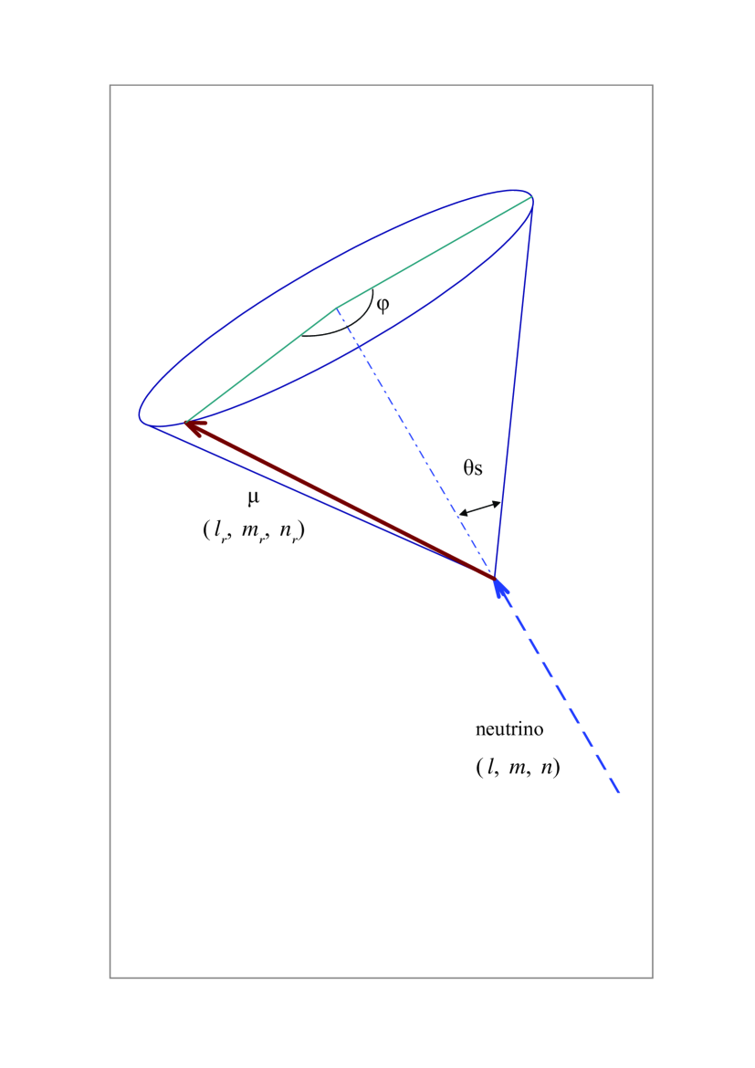
Figure 2: The relation between the direction cosine of the incident neutrino and that of the emitted charged lepton.

Figure 2 shows this relation for muons, in which we can easily understand that the scattering angle $\theta_{\rm s}$ of the emitted lepton (muons here) is greatly influenced not only by the primary neutrino energy but by the emitted lepton’s fractional energy. The effect of scattering angles of the emitted muons (leptons) on the determination of the direction of incident neutrinos therefore cannot be neglected. For a quantitative examination of the scattering angle, we construct the distribution of $\theta_{\rm s}$ of the emitted lepton. Figure 2 gives the distribution function for $\theta_{\rm s}$ of the muon produced in QEL interactions. It can be seen that the muons produced from lower energy neutrinos are scattered over wider angles and that a considerable part of them are scattered even in backward directions. Similar results are obtained for muon anti-neutrinos, electron neutrinos and anti-electron neutrinos.

Also, in a similar manner, we obtain not only the distribution function for the scattering angle of the charged leptons, but also their average values $<\theta_{\rm s}>$ and their standard deviations $\sigma_{\rm s}$. Table 1 shows these quantities for muon neutrinos, anti-muon neutrinos, electron neutrinos and anti-electron neutrinos.

Table 1 shows these quantities for muon neutrinos, muon anti-neutrinos, electron neutrinos and electron anti-neutrinos. From Table 1, Figure 2 and Figure 2, it is clear that for the purpose of establishing the incident neutrino’s direction the scattering angle of the emitted lepton cannot be neglected, especially taking into account the fact that the frequency of the neutrino events with smaller energies is far larger than that of the neutrino events with larger energies due to the steepness of the neutrino energy spectrum. Also, it is clear from Table 1 that there are almost no differences between average scattering angles, and their standard deviations, for muons (anti-muons) and electrons (anti-electrons). The difference of the rest masses between electrons and muons can be completely neglected at the energies under consideration. This fact plays an important role in the discrimination of muons from electron. We shall discuss this matter in Part 2 of our paper .

3.2 The relation between the direction of the emitted lepton and that of the incident neutrinos

In the previous subsection, we point out the non-negligible effect of finite scattering angles of the emitted lepton on the estimation of the direction of the incident neutrinos. Here, we emphasize that the deviation of the directions of emitted leptons from those of the incident neutrinos are enhanced by the effect of the azimuthal angle of the scattering. We examine the effect of the azimuthal angle, $\phi$, and the scattering angle $\theta_{\rm s}$ of an emitted lepton over its zenith angles, $\theta_{\mu({\bar{\mu}})}$, for given zenith angles of the incident neutrinos, $\theta_{\nu({\bar{\nu}})}$ in QEL.

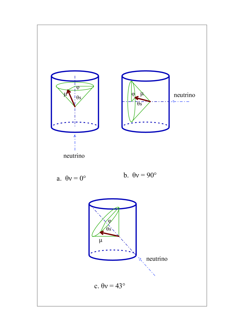
Figure 3: A schematic view of the zenith angles of the charged muon for different zenith angles of the incident neutrino, focusing on their azimuthal angles.

For three typical cases (vertical, horizontal and diagonal), Figure 3 gives a schematic representation of the relationship between the zenith angle of the incident neutrino ,$\theta_{\nu({\bar{\nu}})}$, and the pair of scattering angles, $(\theta_{\rm s},\phi)$ of the emitted muon. The zenith angle of the emitted muon is derived from $\theta_{\nu({\bar{\nu}})}$ and $(\theta_{\rm s},\phi)$ by (A.6) as shown in Appendix A.

From Figure 3-a, it can been seen that the zenith angle $\theta_{\mu({\bar{\mu}})}$ of the emitted lepton is not influenced by its value of $\phi$ for vertically incident neutrinos ($\theta_{\nu({\bar{\nu}})}$ = 0 ), as expected. From Figure 3-b however, it is obvious that the influence of $\phi$ of the emitted leptons on their own zenith angle is the strongest in the case of horizontal incidence of the neutrino ($\theta_{\nu({\bar{\nu}})}$ = 90 ). In that case one half of the emitted leptons are recognized as upward going, while the other half is classified as downward going. In Figure 3-c we give the diagonal case ($\theta_{\nu({\bar{\nu}})}$ = 43 ). It shows the intermediate situation between the vertical and the horizontal. In the following, we examine the cases for vertical, horizontal and diagonal incidence of neutrinos with different energies, $E_{\nu({\bar{\nu}})}$ = 0.5 GeV, 1 GeV and 5 GeV as typical cases.

(a)                                                (b)                                                (c)

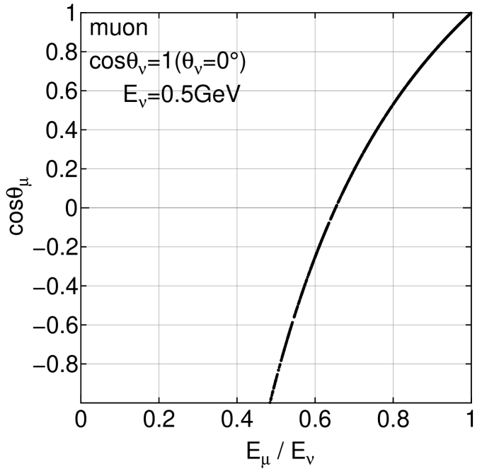
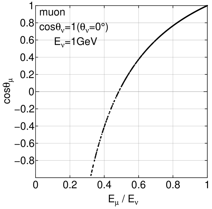
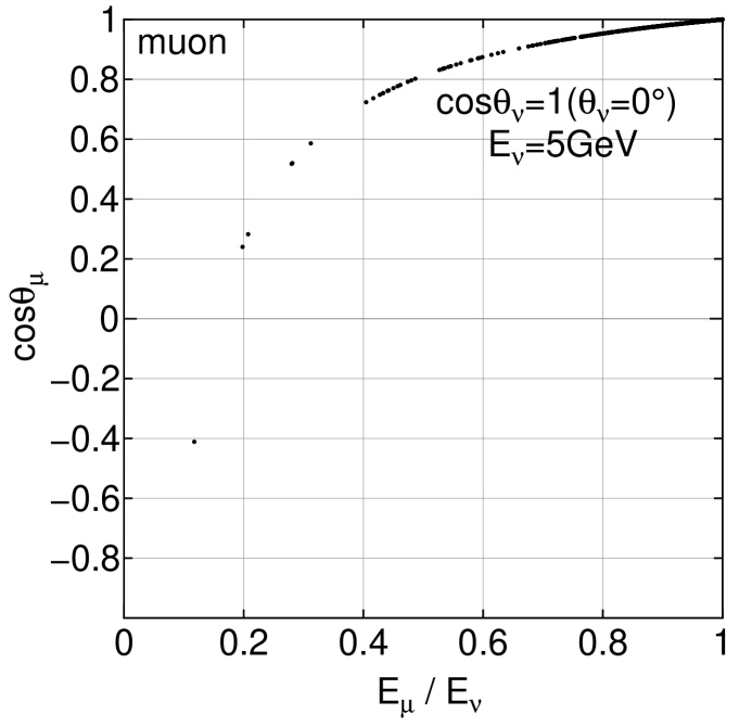
Figure 4: The scatter plots of the fractional energies of the produced muons and their zenith angles for vertically incident muon neutrinos with 0.5 GeV, 1 GeV and 5 GeV, respectively. The sampling number is 1000 in each case.

(a)                                                (b)                                                (c)

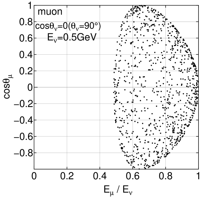
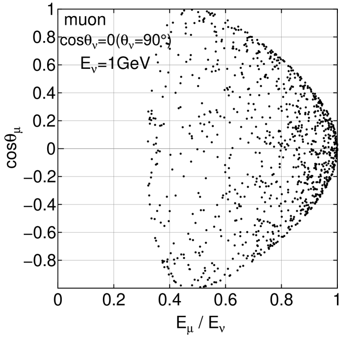
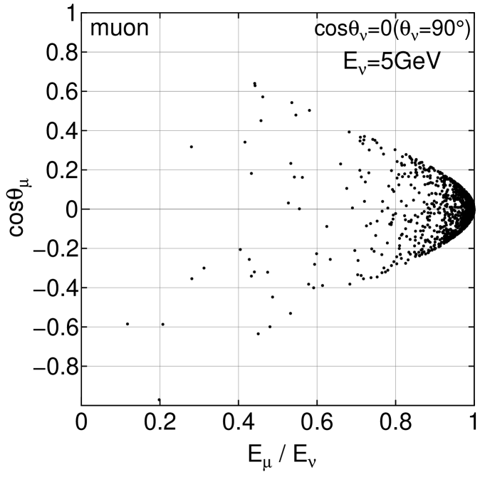
Figure 5: The scatter plots of the fractional energies of the produced muons and their zenith angles for horizontally incident muon neutrinos with 0.5 GeV, 1 GeV and 5 GeV, respectively. The sampling number is 1000 in each case.

(a)                                                (b)                                                (c)

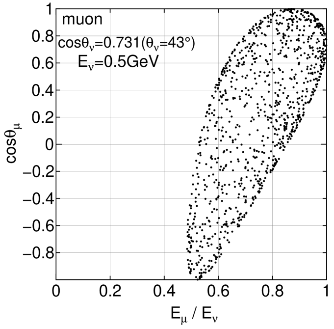
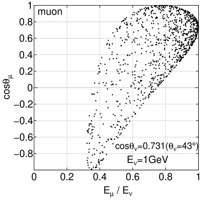
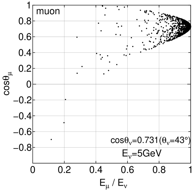
Figure 6: The scatter plots of the fractional energies of the produced muons and their zenith angles for diagonally incident muon neutrinos with 0.5 GeV, 1 GeV and 5 GeV, respectively. The sampling number is 1000 in each case.

3.3 Dependence of the width of the zenith angle distribution of emitted leptons on their energy for different incident directions and energies of the neutrinos

The detailed procedure for our Monte Carlo simulation is described in Appendix A. We give the scatter plots between the fractional energy of the emitted muons and their zenith angle for a definite zenith angle of the incident neutrino with different energies in Figures 6 to  6. In Figure 6, we give the scatter plots for vertically incident neutrinos with different energies 0.5, 1 and 5 GeV. In this case, the relations between the emitted energies of the muons and their zenith angles are unique, which comes from the definition of the zenith angle of the emitted lepton. However, the densities (frequencies of the event numbers) along each curve are different in position to position and depend on the energies of the incident neutrinos. Generally speaking, densities along the curves become greater toward $cos\theta_{\mu(\bar{\mu})}$= 1. In this case, $cos\theta_{\mu(\bar{\mu})}$ is never influenced by the azimuthal angle in the scattering by the definition². On the contrary, it is shown in Figure 6 that the horizontally incident neutrinos give the widest zenith angle distribution for the emitted muons with the same fractional energies, an effect exclusively due to the azimuthal angle. The lower the energies of the incident neutrinos, the wider the spreads of the scattering angles of emitted muons $\theta_{\mu(\bar{\mu})}$, which leads to wider zenith angle distributions for the emitted muons and, therefore, we cannot estimate the directions of the incident neutrinos from the directions of the emitted leptons, especially in lower energies. As is easily understood from Figure 6, the diagonally incident neutrinos give the intermediate zenith angle distributions for the emitted muons between those for vertically incident neutrinos and those for horizontally incident neutrinos. It should be noted from the figures that the influence of the azimuthal angles in QEL on the cosines of the zenith angle of the incident neutrino exists for the most inclined neutrinos, even when the scattering angle due to QEL is small.

(a)                                                (b)                                                (c)

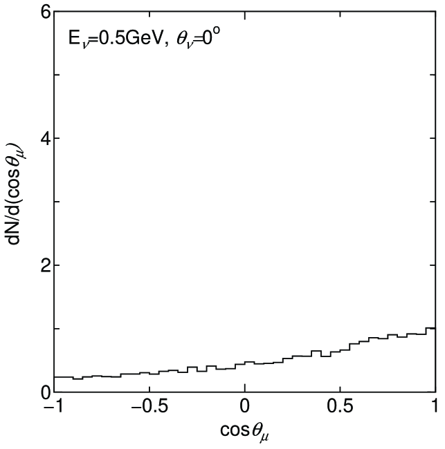
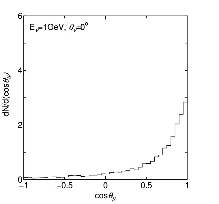
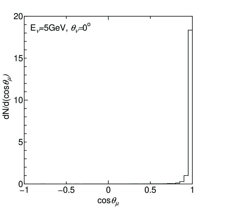
Figure 7: The zenith angle distribution of the muons for vertically incident muon neutrinos with 0.5 GeV, 1 GeV and 5 GeV, respectively. The sampling number is 10000 in each case.

(a)                                                (b)                                                (c)

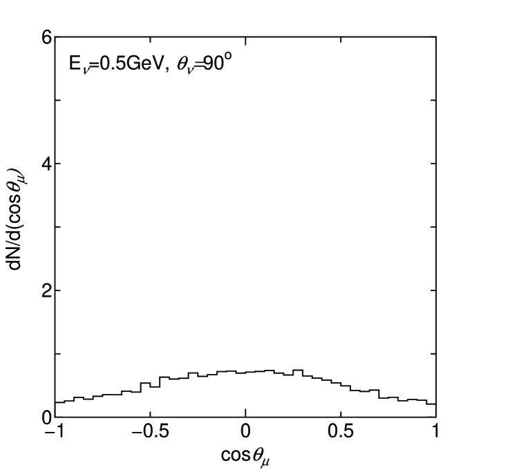
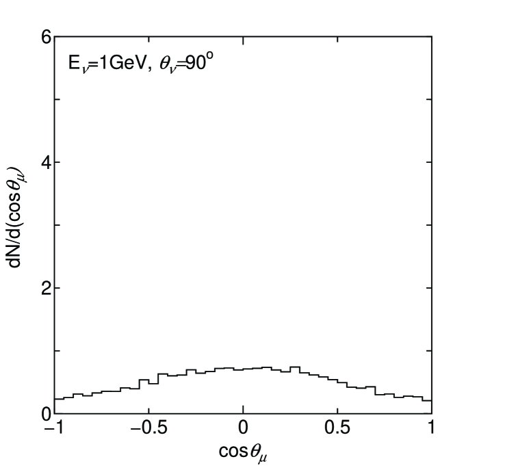
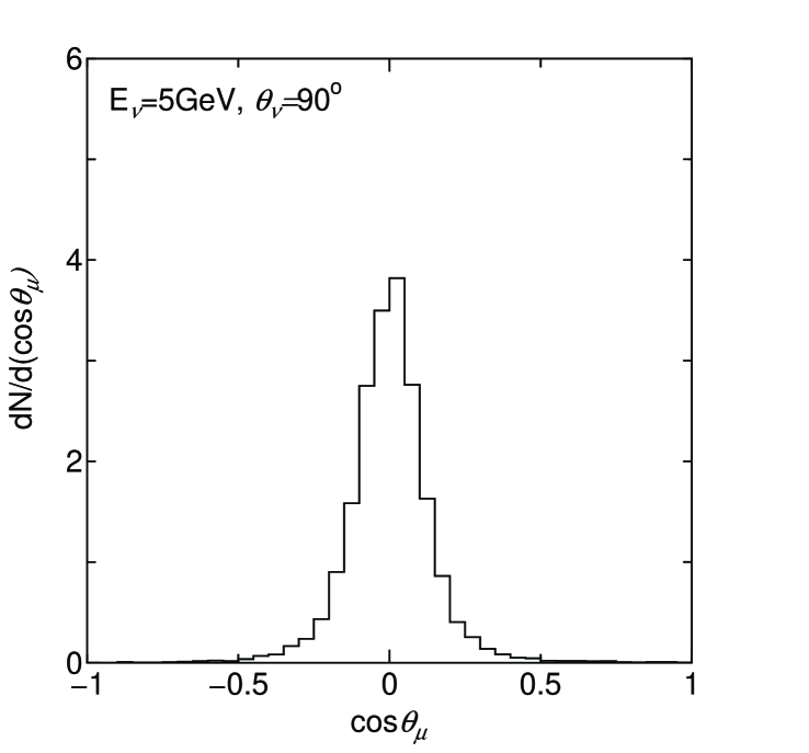
Figure 8: The zenith angle distribution of the muons for horizontally incident muon neutrinos with 0.5 GeV, 1 GeV and 5 GeV, respectively. The sampling number is 10000 in each case.

(a)                                                (b)                                                (c)

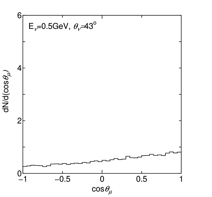
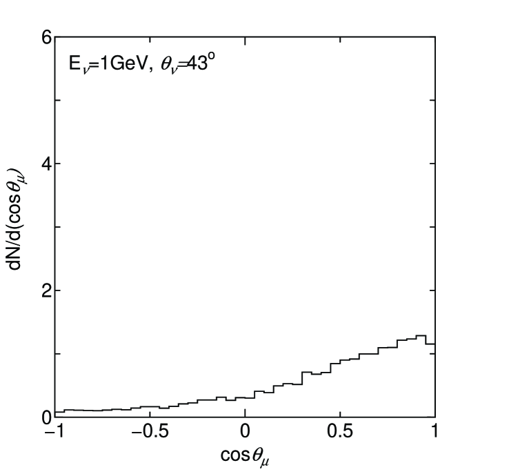
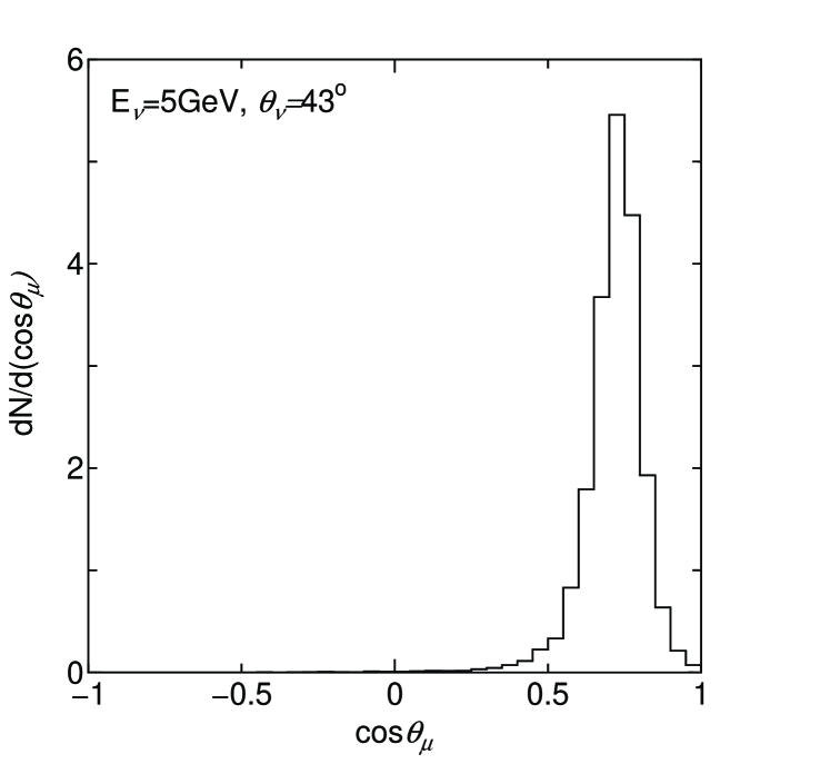
Figure 9: The zenith angle distribution of the muons for diagonally incident muon neutrinos with 0.5 GeV, 1 GeV and 5 GeV, respectively. The sampling number is 10000 in each case.

3.4 Zenith angle distribution of the emitted leptons for different incident directions and energies of the neutrinos

In Figures 9 to 9, we show distributions of the zenith cosine of the emitted muons for different incident directions and different incident energies of neutrinos. In Figures 9(a) to 9(c), we give the zenith cosine distributions of the emitted muons for the case of vertically incident neutrinos with different energies, $E_{\nu}$= 0.5, 1 and 5 GeV. Comparing the case for $E_{\nu}$= 0.5 GeV with that for $E_{\nu}$= 5 GeV, we see big difference between the two. The scattering angle of the emitted muon for 5 GeV neutrinos is relatively small (see also Table 1), so that the emitted muons keep roughly the same directions as their original neutrinos. In this case, the effect of their azimuthal angle on the resulting zenith angle is also smaller. However, in the case of $E_{\nu}$= 0.5 GeV, the dominant energy for the neutrino events which are fully contained in the detector, not a small percentage of the muons are emitted in the backward direction due to large angle scattering. The most frequent occurrence in the backward direction of the emitted muon appears in the horizontally incident neutrino as shown in Figures 9(a) to  9(c). In this case, the zenith angle distribution of the emitted muon should be symmetrical with regard to the horizontal direction. Comparing the case for 5 GeV with those both for 0.5 GeV and for 1 GeV, even 1 GeV incident neutrinos lose almost their memory of the incident direction. Figures 9(a) to 9(c) for diagonally incident neutrinos tell us that the situation for the diagonal case lies between the case for the vertically incident neutrinos and that for horizontally incident ones. From Figures  9(a) to 9(c), it is clear that the scattering angles of emitted muons affect the determination of zenith angles of incident neutrinos. The effect is enhanced by their azimuthal angles, particularly for more inclined directions of the incident neutrinos.

(a)                                            (b)                                            (c)

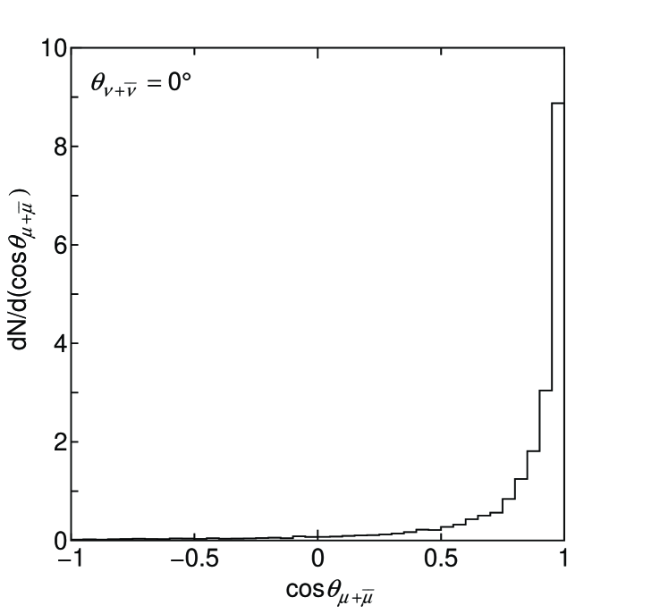
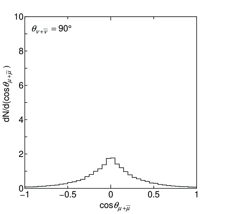
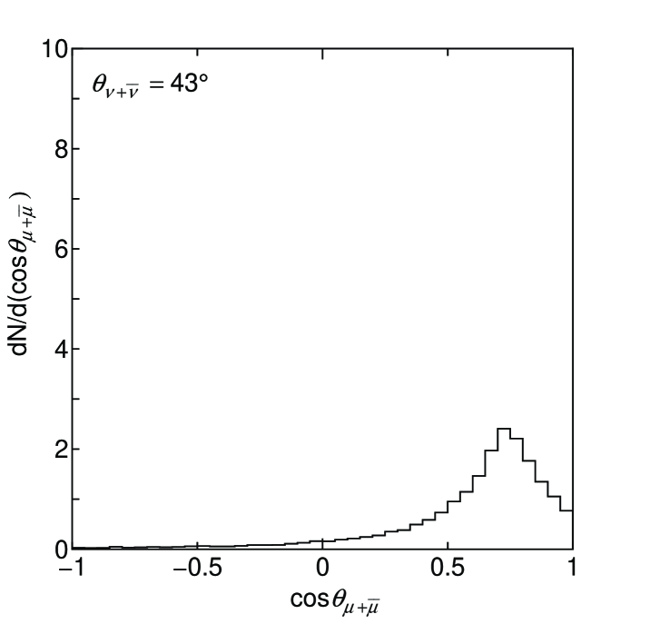
Figure 10: The zenith angle distribution for the sum of $\mu^{-}$ and $\mu^{+}$ for incident neutrinos, $\bar{\nu}$ and $\nu$ for the vertical, horizontal and diagonal directions, respectively (see Figure 3). The overall neutrino spectra at the Kamioka site are taken into account. The sampling number is 10000 in each case.

3.5 Zenith angle distribution of Fully Contained Events for a given zenith angle of the incident neutrino, taking their energy spectrum into account

In the previous subsections we discuss the relation between the zenith angle distribution of the incident neutrino and that of the emitted muons produced by the neutrinos for three different directions and three different energies of incident neutrinos. In order to apply our inspection to the real experiment using the underground detectors, we must consider the effect of the energy spectrum of the incident neutrinos. Here, we adopt Honda’s spectrum[2] for incident neutrino energy. Details of the Monte Carlo simulations for this purpose are given in Appendix B. In Figure 10, we give the zenith angle distributions of the sum of $\mu^{+}$($\bar{\mu}$) and $\mu^{-}$ and for a given incident zenith angle of $\nu_{\bar{\mu}}$ and $\nu_{\mu}$, taking into account the different primary neutrino energy spectra for different directions at the underground detector at the Kamioka site [2]. It is clear from these figures that the zenith angles of the Fully Contained Events are greatly influenced by the scattering angle of emitted leptons. The effect becomes much more in case of inclined events if we take the azimuthal angle into consideration.

4 The correlation between $cos\theta_{\nu(\bar{\nu})}$ (or $L_{\nu(\bar{\nu})}$) and $cos\theta_{\mu(\bar{\mu})}$ (or $L_{\mu(\bar{\mu})}$), and the correlation between $E_{\nu(\bar{\nu})}$ and $E_{\mu(\bar{\mu})}$

In this section and section 5, we give a part of the results obtained from the $L/E$ analysis for QEL events among the Fully Contained Events with our Computer Numerical Experiment. For the execution of our experiment, we borrow necessary data from the Super-Kamiokande Collaboration[1], the detector geometry, the duration of 1489.2 live days, oscillation parameters, $sin^{2}2\theta=1.0$ and $\Delta m^{2}=2.4\times 10^{-3}\rm{eV^{2}}$, and the incident neutrino spectrum[2]. Here, we examine $cos\theta_{\nu(\bar{\nu})}$ (or $L_{\nu(\bar{\nu})}$) and $cos\theta_{\mu(\bar{\mu})}$ (or $L_{\mu(\bar{\mu})}$), and the correlation between $E_{\nu(\bar{\nu})}$ and $E_{\mu(\bar{\mu})}$ in the QEL events among the Fully Contained events, where $cos\theta_{\nu(\bar{\nu})}$, $cos\theta_{\mu(\bar{\mu})}$, $L_{\nu(\bar{\nu})}$ and $L_{\mu(\bar{\mu})}$ are the zenith cosine of the incident neutrino and that of the emitted muon, the corresponding flight path length of the incident neutrino and that of the emitted muon, respectively.

In the following and subsequent sections, we examine the validity of Eq.(2) in the QEL events among the Fully Contained Events. There are two possibilities in order that Eq.(2) is valid.

• : The relations of both $L_{\nu}\approx L_{\mu}$and $E_{\nu}\approx E_{\mu}$ hold good.

• : In spite of the failure of Case A, Eq.(2) holds due to unknown reasons.

First of all, we examine CASE A.

4.1 The Correlation between $cos\theta_{\nu(\bar{\nu})}$ and $cos\theta_{\mu(\bar{\mu})}$

Here, we examine the correlation between $cos\theta_{\nu}$ and $cos\theta_{\mu}$ for the neutrino events concerned (QEL events) by the computer numerical experiment assuming live days same to the real ones of the underground experiment[1] and the incident neutrino energy spectrum as a function of zenith angle as in [2]. The details are given in Appendix C. In order to obtain the zenith angle distribution of the emitted leptons arising from the incident neutrinos, we divide the range of cosine of the zenith angle of the incident neutrino into twenty regular intervals from $cos\theta_{\nu}=-1$ (downward) to $cos\theta_{\nu}=1$ (upward). For given interval of $cos\theta_{\nu}$, we carry out the exact Monte Carlo simulation, starting to sample neutrino events in a stochastic manner from the incident neutrino energy spectrum for given $cos\theta_{\nu}$, the cosine of the zenith angles of the incident neutrinos, and obtain finally $cos\theta_{\mu}$, the cosine of the zenith angles of the emitted leptons.

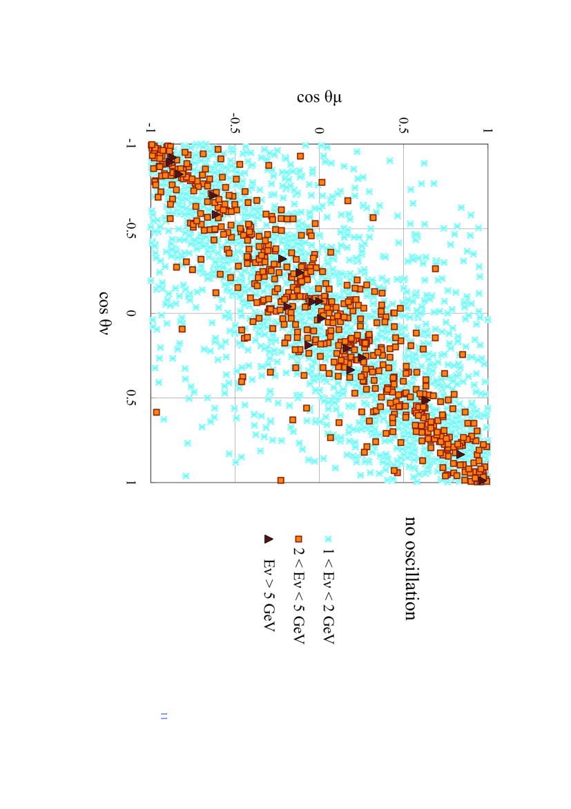
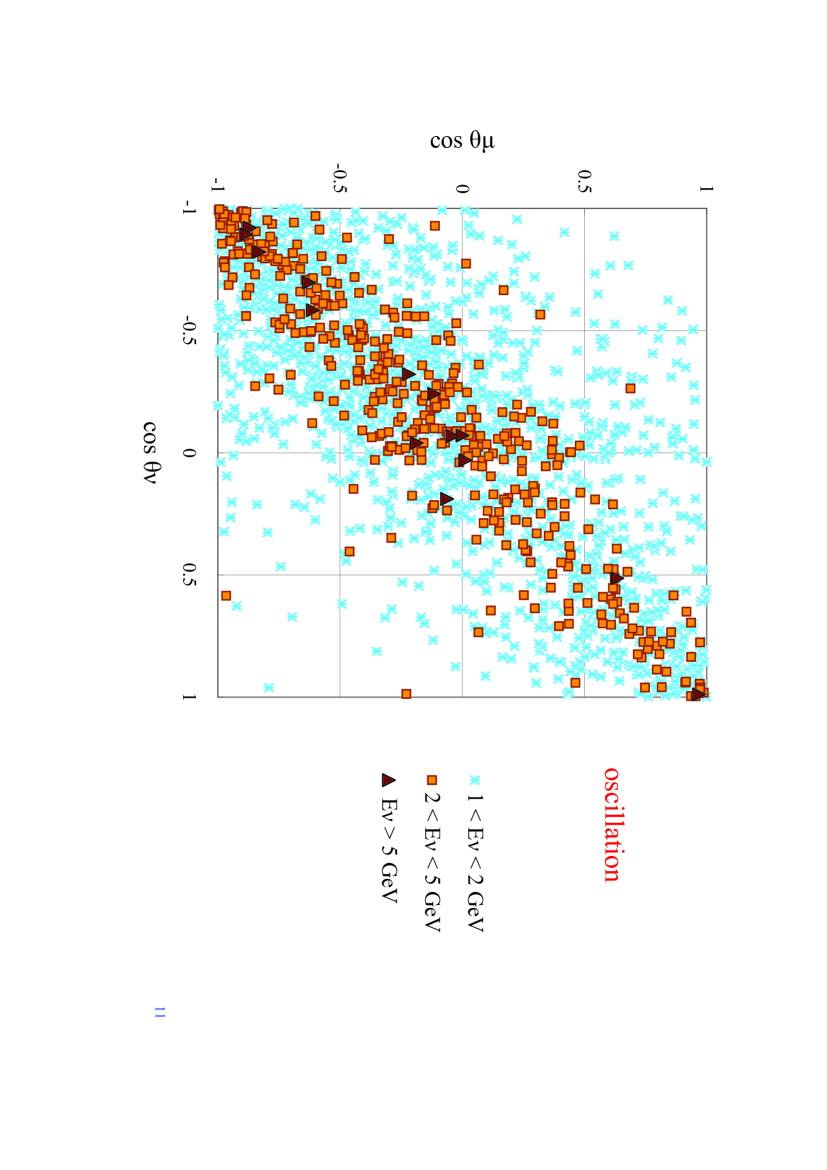
Figure 11: The correlation diagram between $\cos{\theta}_{\nu}$ and $\cos{\theta}_{\mu}$ for null oscillations for different neutrino energy regions.

Figure 12: The correlation diagram between $\cos{\theta}_{\nu}$ and $\cos{\theta}_{\mu}$ for oscillations for different neutrino energy regions.

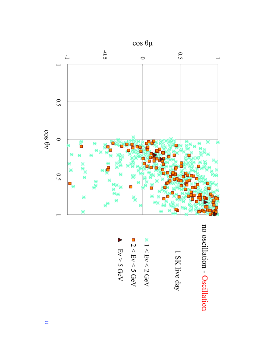
Figure 13: The correlation diagram between $\cos{\theta}_{\nu}$ and $\cos{\theta}_{\mu}$ for those events which exist for null oscillations but disappear due to oscillations for different neutrino energy regions.

4.1.1 The case without neutrino oscillations

In Figure 12 we give the correlation diagram between $\cos{\theta}_{\nu}$ and $\cos{\theta}_{\mu}$ in case of no neutrino oscillation for 1489.2 live days.

In the figure, we plot data using different symbols for three different primary energies, $E_{\nu}>$ 5 GeV , 2 $<E_{\nu}<$ 5 GeV and 1 $<E_{\nu}<$ 2 GeV, in order to examine the influence of the incident energies on the correlation between $\cos{\theta}_{\nu}$ and $\cos{\theta}_{\mu}$. The neutrino events of $E_{\nu}>$ 5 GeV are distributed roughly on the line $\cos{\theta}_{\nu}=\cos{\theta}_{\mu}$. This reflects the fact that the emitted leptons in such higher energy interactions are produced with smaller scattering angles so that they are less influenced by their azimuthal angles (see Table 1, Figure 2, Figures 6(c) to 6(c)). In this energy region the directions of the incident neutrinos can be approximately determined by those of the emitted muons. The neutrino events of 2 $<E_{\nu}<$ 5 GeV are also distributed along the line $\cos{\theta}_{\nu}=\cos{\theta}_{\mu}$, but the correlation is weaker than in the case of neutrino events of $E_{\nu}>$ 5 GeV. In this energy region the direction of the incident neutrinos determined by those of the emitted muons has larger uncertainties. The influence of such larger uncertainty on the $L/E$ distribution must be carefully examined. In contrast to these higher energy ranges, $E_{\nu}>$ 2 GeV, the neutrino events of lower energies, 1 $<E_{\nu}<$ 2 GeV, are scattered out widely around the line $\cos{\theta}_{\nu}=\cos{\theta}_{\mu}$. The fact that the relation $\cos{\theta}_{\nu}\approx\cos{\theta}_{\mu}$ does not hold, as seen in the figure, plays a decisively important role in the $L/E$ analysis (see section 4.2). The influence of the emitted muons’ directions on determining those of the incident neutrinos will be carefully examined in the subsequent papers, because it is closely related to the maximum oscillation in the survival probability.

It is interesting to classify the events in Figure 12 into the following four sectors with the regard to the origin ($\cos{\theta}_{\nu}=0,\cos{\theta}_{\mu}=0$).

• The first sector where $\cos{\theta}_{\nu}>0$ and $\cos{\theta}_{\mu}>0$. In this sector we recognize that the incident neutrinos go upward ($\cos{\theta}_{\nu}>0$) and the emitted leptons also go upward ($\cos{\theta}_{\mu}>0$) in the interaction. Namely, the scattered leptons are produced in the forward direction by the upward neutrinos (see footnote 2).

• The second sector where $\cos{\theta}_{\nu}<0$ and $\cos{\theta}_{\mu}>0$. In this sector we recognize that the incident neutrinos go downward ($\cos{\theta}_{\nu}<0$) but the emitted leptons go upward ($\cos{\theta}_{\mu}>0$) in the interaction. Such situations may occur due to two different causes. One is that the emitted leptons are scattered in the backward directions (backward scattering, see Figures 2 and 2), while the other is that the emitted leptons are scattered forward by the downward neutrinos, but they look like backward scattering due to the azimuthal angle effect (see Figure 3(b) and 3(c)).

• The third sector where $\cos{\theta}_{\nu}<0$ and $\cos{\theta}_{\mu}<0$. In this sector we recognize that the incident neutrinos go downward and the emitted leptons are scattered forward in the interaction.

• The fourth sector where $\cos{\theta}_{\nu}>0$ and $\cos{\theta}_{\mu}<0$. In this sector we recognize that the incident neutrinos go upward ($\cos{\theta}_{\nu}>0$) and the emitted leptons go downward ($\cos{\theta}_{\mu}<0$) in the interaction. These situations also may occur due to different causes. One is that the emitted leptons are scattered backward (backward scattering, see Figures   2 and 2) and the other is that the emitted leptons are scattered forward, but they looks like backward scattering due to the azimuthal angle effect (see Figure 3(b) and 3(c)).

We can see in Figure 12 that the distribution of the neutrino events in the first sector and that in the third sector is essentially symmetrical and that in the second sector and that in the fourth sector is also symmetrical. Such symmetry is easily understood from the fact that the mean free paths of the neutrino interactions in the energy region smaller than 10 GeV, which corresponds to the maximum energy for Fully Contained Events, is far larger than the diameter of the Earth and consequently neutrino fluxes for the interaction are independent of the thickness traversed through the Earth by the incident neutrinos. The reason for the smaller number of the events in the second sector (or the fourth sector), compared with that in the third sector (or the first sector) is that the probability of backward scattering of muons is smaller than that of forward scattering. The existence of such symmetries gives certain evidence that our Computer Experiment is carried out in a correct manner.

4.1.2 The case with neutrino oscillations

In Figure 12, we give the corresponding correlation diagram for the case with neutrino oscillations, which should be compared with Figure 12(no oscillations). In the case of the presence of neutrino oscillations, the symmetries between the first and third sectors, and those between the second and fourth sectors, are lost due to the neutrino oscillation effect. This is because the neutrino flux of the upward neutrinos is reduced compared with that of the downward neutrinos due to the survival probability (See Eq.(3.1)). Of course, the destruction of these symmetries depends on the values of the oscillation parameters, $\Delta m^{2}$ and $sin^{2}2\theta$ . In Figure 13, we show the disappeared events which are the result of neutrino oscillations, i.e. the neutrino events resulting from subtraction of Figure 12 from Figure 12). It should be noticed from the figure that the disappeared events are concentrated in the first sector and the fourth sector and that almost no disappeared event are to be found in the second sector and the third sector. The reasons are as follows: The neutrino events in the second sector and the third sector are due to the downward neutrinos which suffer almost no oscillation effect. Consequently, there are almost no disappeared events, as shown in Figure 12. On the contrary, neutrino events in the first sector and the fourth sector are due to the upward neutrinos, which can be affected by the neutrino oscillation. The neutrino events in the first sector are due to the forward scattering and those in the fourth sector are due to the backward scattering and consequently the number of the neutrino event in the first sector is larger than that in the fourth sector, because the probability of forward scattering is larger than for backscattering (see Figure 2).

This situation is closely related to the adoption of the specified neutrino oscillation parameters of $\Delta m^{2}$ and $sin^{2}2\theta$ . The influence of the energies of the incident neutrinos on the correlation between $cos\theta_{\nu(\bar{\nu})}$ and $cos\theta_{\mu(\bar{\mu})}$ with oscillations is essentially the same as in the case without oscillations. The difference comes from the event rate due to neutrino oscillation effect.

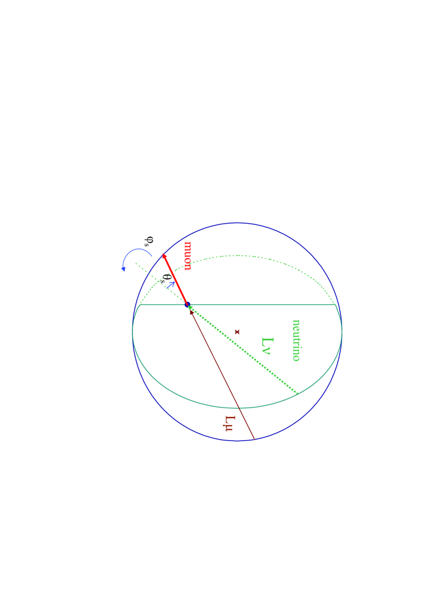
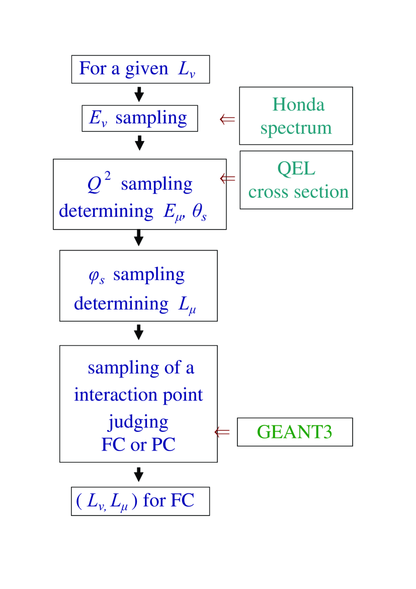
Figure 14: Schematic view of relations among $L_{\nu}$, $L_{\mu}$, $\theta_{s}$ and $\phi_{s}$ .

Figure 15: The procedure for our numerical experiment for obtaining $L_{\mu}$ from a given $L_{\nu}$.

4.2 The correlation between $L_{\nu}$ and $L_{\mu}$

What we need for our argument on the $L/E$ analysis of neutrino oscillations are $L_{\nu}$ and $L_{\mu}$, but not $cos\theta_{\nu}$ and $cos\theta_{\mu}$, Therefore, we must transform $cos\theta_{\nu}$ and $cos\theta_{\mu}$ to $L_{\nu}$ and $L_{\mu}$. The transformations are carried out by the following equations.

$$L_{\nu}=R_{g}\times(r_{SK}cos\theta_{\nu}+\sqrt{r_{SK}^{2}cos^{2}\theta_{\nu}+1-r_{SK}^{2}})\,\,\,(7-1)$$

$$L_{\mu}=R_{g}\times(r_{SK}cos\theta_{\mu}+\sqrt{r_{SK}^{2}cos^{2}\theta_{\mu}+1-r_{SK}^{2}})\,\,\,(7-2)$$

where $R_{g}$ is the radius of the Earth and $r_{SK}=1-D_{SK}/R_{g}$, $D_{SK}$, is the depth of the underground detector from the surface of the Earth[1]. In Figure 15, we give schematically the mutual relation among $L_{\nu}$, $L_{\mu}$, $\theta_{s}$(the scattering angle due to QEL) and $\phi_{s}$ (the azimuthal angle in QEL). As we are exclusively interested in the analysis of Fully Contained Events, we give the procedure for getting the correlation between $L_{\nu}$ and $L_{\mu}$ for those events in Figure 15.

Figures 18, 18 and 18 show correlation diagrams for $L_{\nu}$ and $L_{\mu}$ obtained by applying the above transformation, eqs. (7-1) and (7-2), to the events shown in Figures 12, 12 and 13.

The correlation diagrams expressed by $L_{\nu}$ and $L_{\mu}$ are classified into four sectors, just the same as those used for the $cos\theta_{\nu}-cos\theta_{\mu}$ plot. Here the coordinate axes, which correspond to both $cos\theta_{\nu}=0$ and $cos\theta_{\mu}=0$ in Figures 12, 12 and 13, are $L_{\nu}=L_{h}$ and $L_{\mu}=L_{h}$, where the numerical value is $L_{h}\approx 138$ km, the distance from the underground detector to the edge of the Earth in the horizontal direction. We now examine the four sectors in the $L_{\nu}-L_{\mu}$ plot (above the horizon or below the horizon), as we examined the four sectors in Figures 12, 12 and 13, in the $cos\theta_{\nu}-cos\theta_{\mu}$ plot (downward or upward). Taking $L_{\nu}=L_{\mu}\sim 138$ km as the origin of the coordinates, each sector is classified as follows:

• The first sector where both $L_{\nu}>L_{h}$ and $L_{\mu}>L_{h}$, respectively. This sector corresponds exactly to the first sector in Figures 12, 12 and 13, in the $cos\theta_{\nu}-cos\theta_{\mu}$ plot.

• The second sector where $L_{\nu}<L_{h}$ and $L_{\mu}>L_{h}$. This sector corresponds exactly to the second sector in Figures 12, 12 and 13, in the $cos\theta_{\nu}-cos\theta_{\mu}$ plot.

• The third sector where $L_{\nu}<L_{h}$ and $L_{\mu}<L_{h}$. This sector corresponds exactly to the third sector in Figures 12, 12 and 13, in the $cos\theta_{\nu}-cos\theta_{\mu}$ plot.

• The fourth sector where $L_{\nu}>L_{h}$ and $L_{\mu}<L_{h}$. This sector corresponds exactly to the fourth sector in Figures 12, 12 and 13, in the $cos\theta_{\nu}-cos\theta_{\mu}$ plot.

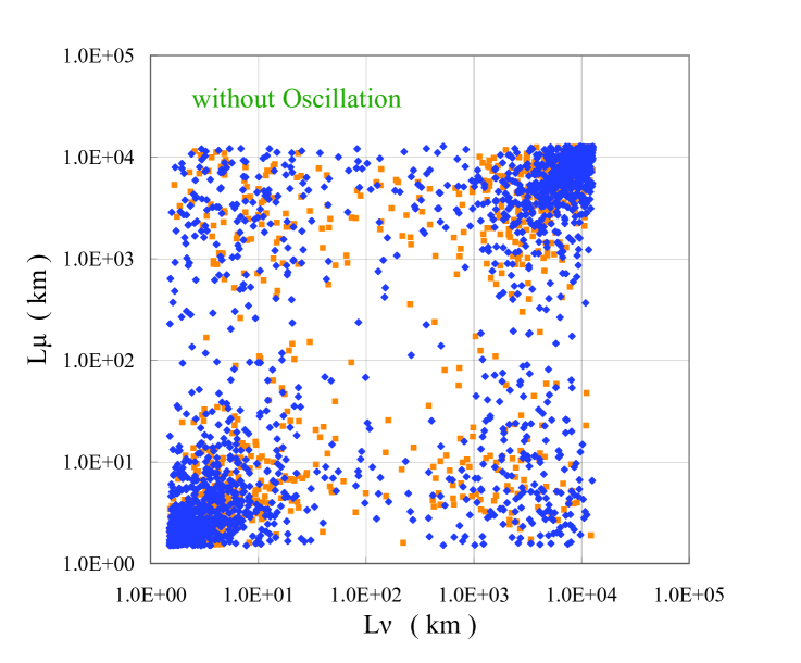
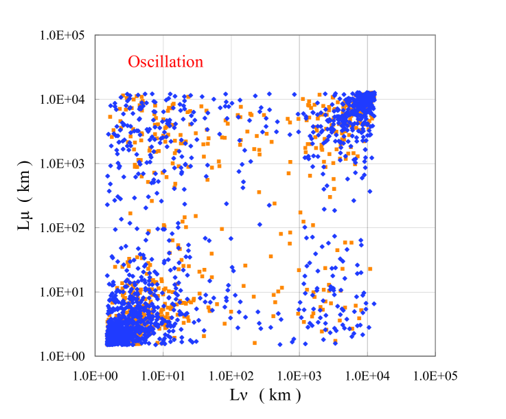
Figure 16: The correlation diagram for $L_{\nu}$ and $L_{\mu}$ without oscillations for 1489.2 live days of observation. The blue points and orange points denote neutrino events and ani-neutrino events, respectively.

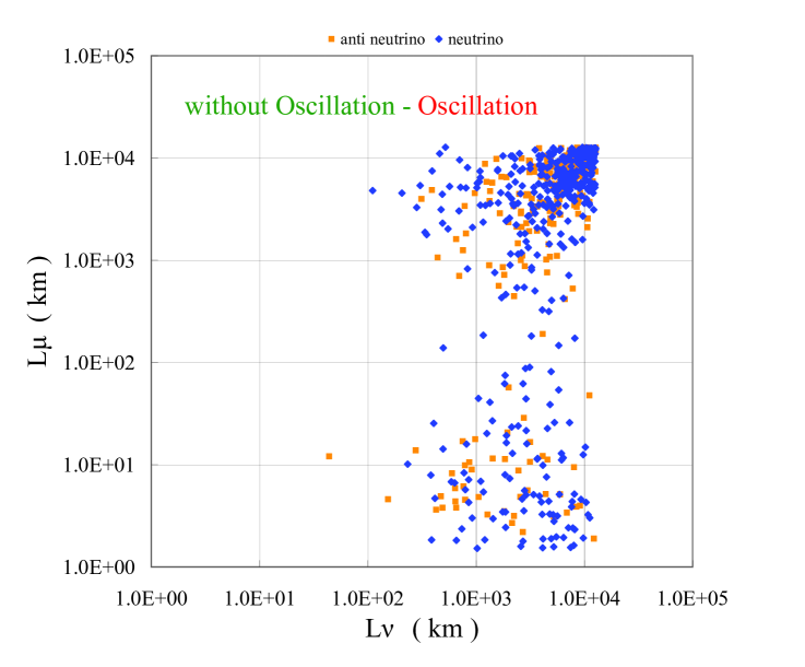
Figure 17: The correlation diagram for $L_{\nu}$ and $L_{\mu}$ with oscillations for 1489.2 live days of observation. The blue points and orange points denote neutrino events and ani-neutrino events, respectively.

Figure 18: The correlation diagram for $L_{\nu}$ and $L_{\mu}$ for those events which exist in null oscillations but disappear due to oscillations for 1489.2 live days of observation. The blue points and orange points denote neutrino events and ani-neutrino events, respectively.

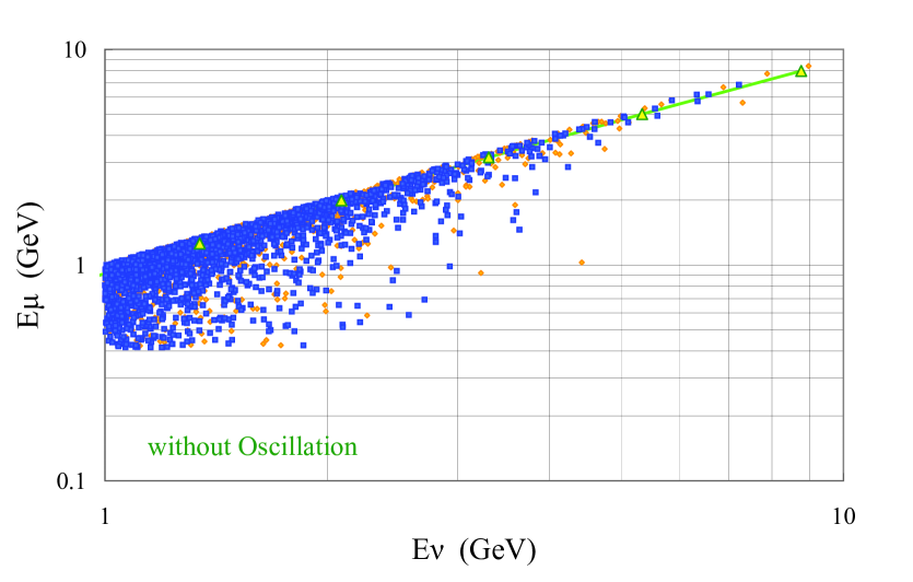
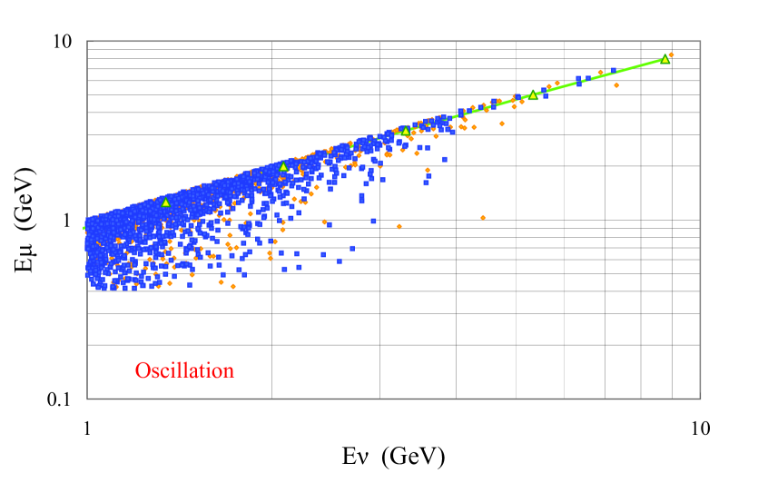
(a)                                                                      (b)

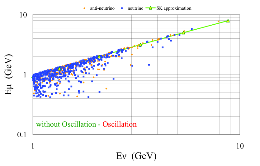
(c)

Figure 19: The correlation diagram for $E_{\nu}$ and $E_{\mu}$, (a)without oscillations, (b)with oscillations and (c)for those events which exist in null oscillations but disappear due to oscillations, for 1489.2 live days of observation, respectively. The solid line denotes the polynomial expression used by the Super-Kamiokande Collaboration.

4.2.1 The case without neutrino oscillations

In Figure 18, we give the correlation between $L_{\nu}$ and $L_{\mu}$ in the case without oscillations. The figure is another expression of Figure 12. The symmetry between the first sector and the third sector, and that between the second and the fourth with regard to the origin ($L_{\nu}=L_{\mu}\sim 138$km) are retained just as in Figure 12 with regard to the origin ($\cos{\theta}_{\nu}=0,\,\cos{\theta}_{\mu}=0$) for the same reason. The density of the number of events around the origin in the $L_{\nu}-L_{\mu}$ plot (Figure 18) looks to be far smaller than that in $\cos{\theta}_{\nu}-\cos{\theta}_{\mu}$ plot (Figure 12). This is simply due to the fact that the region of $\cos{\theta}_{\nu}$($\cos{\theta}_{\nu}$) $\sim 0$ becomes very wide when $L_{\nu}$ ($L_{\mu}$) are expressed on a log-scale (see Eq.(7.1) and (7.2)).

4.2.2 The case with neutrino oscillations

In Figure 18, we give the correlation between $L_{\nu}$ and $L_{\mu}$ in the case without oscillations. The figure is another expression of Figure 12. The symmetry which exists in Figure 18 is lost here in Figure 18 due to the neutrino oscillations just as was the case in Figure 12. Also, the situation for the disappeared events which is shown in Figure 18 is exactly the same as that shown in Figure 13. It is easily understood from Figure 18 that the disappeared events are found in the region $L_{\nu}>L_{h}$ (from under the horizon) and they are found mostly in the region $L_{\mu}>L_{h}$ (forward scattering) while they are scarcely found in the region $L_{\mu}<L_{h}$ (backward scattering). Thus, we reach the important conclusion from Figure 18 to 18 that the relation of $L_{\nu}\approx L_{\mu}$ does not hold, irrespective of whether there are oscillations or not, just as $\cos{\theta}_{\nu}\neq\cos{\theta}_{\nu}$ shown in Figures 12 to 13.

Here, we return to the question of the validity of Eq.(2). The question whether $L_{\nu}\approx L_{\mu}$ or not is classified, furthermore, into two sub-questions. One is whether the relation of $L_{\nu}\approx L_{\mu}$ holds for each event and the other is whether the relation holds only statistically. From Figures 18 to 18 we see that the above relation does not hold even in the statistical sense, because $L_{\mu}$ is distributed widely for any given $L_{\nu}$. We can conclude that one of the necessary conditions for the validity of Eq.(2) in the case A does not hold.

4.3 The correlation between $E_{\nu}$ and $E_{\mu}$

Now, we examine another necessary condition around $E_{\nu}$ and $E_{\mu}$. In Figures 19, we give correlation diagrams of $E_{\nu}$ and $E_{\mu}$ for the events. The solid line in the figures is a polynomial equation, which gives the relationship between $E_{\nu}$ and $E_{\mu}$, used by the Super-Kamiokande collaboration[5]. In Figure 19-(a) we give the correlation for the events without oscillations, while in Figure 19-(b) we give those for the events with oscillations. In Figure 19-(c), we give the correlation for the absent events due to neutrino oscillations. It is clear from these figures that the lower the energy of the incident neutrinos, the stronger the fluctuations in the emitted muon energy, which is easily conjectured from Figures 2 and 2, and Table 1. Then we can conclude that $E_{\nu}\approx E_{\mu}$ does not hold irrespective of oscillations or no oscillations, just as in the case of the directions.

4.4 Summary of section 4

There is a distinctive difference in their respective properties between $L_{\nu}$ versus $L_{\mu}$ and $E_{\nu}$ versus $E_{\mu}$ from the point of view of their correlations. It is clear from the comparison of Figures 18 to 18 16, 17 and 18 with Figures 19-(a), 19-(b) and 19-(c) that the difference of muon data from neutrino data is far larger in the flight path lengths than in the energies. Consequently, we may approximate $E_{\nu}$ by $E_{\mu}$ legitimately, but it is impossible to approximate $L_{\nu}$ by $L_{\mu}$ in any sense. The incapability of the replacement of $L_{\nu}$ by $L_{\mu}$ comes from the fact that the azimuthal angle of the emitted muons plays an essential role in the transformation of $L_{\nu}$ from $L_{\mu}$. In conclusion, we can definitely say that neither $L_{\nu}\approx L_{\mu}$ nor $E_{\nu}\approx E_{\mu}$ can be assumed in the analysis of Fully Contained neutrino events, so that we finally exclude the Case A.

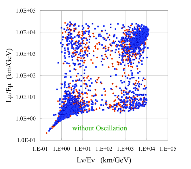
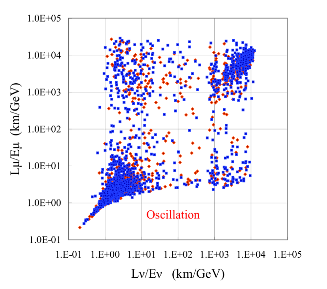
Figure 20: The correlation diagram for $L_{\nu}/E_{\nu}$ and $L_{\mu}/E_{\mu}$ without oscillations for 1489.2 live days of observation. The blue points and orange points denote neutrino events and ani-neutrino events, respectively.

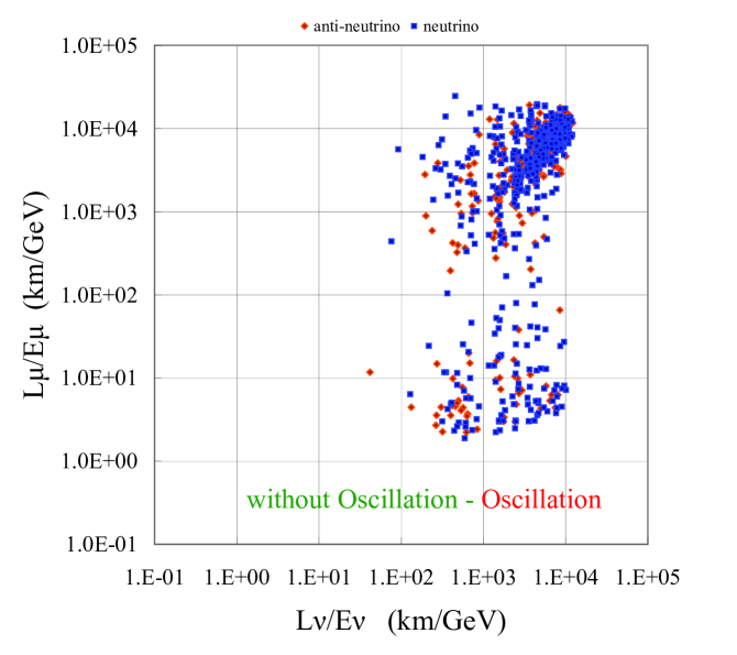
Figure 21: The correlation diagram for $L_{\nu}/E_{\nu}$ and $L_{\mu}/E_{\mu}$ with oscillations for 1489.2 live days of observation. The blue points and orange points denote neutrino events and ani-neutrino events, respectively.

Figure 22: The correlation diagram for $L_{\nu}/E_{\nu}$ and $L_{\mu}/E_{\mu}$ for those events which exist in null oscillations but disappear due to oscillations for 1489.2 live days of observation. The blue points and orange points denote neutrino events and ani-neutrino events, respectively.

5 The correlation between $L_{\nu}/E_{\nu}$ and $L_{\mu}/E_{\mu}$

In Figures 22, 22 and 22, we give the correlation diagram between $L_{\nu}/E_{\nu}$ and $L_{\mu}/E_{\mu}$ for the events without oscillations, with oscillations, and the disappeared events, respectively.

We can give a clear physical image in each section from the first to the fourth with regard to the origin ($L_{\nu}=L_{\mu}\sim 138$ km) in the $L_{\nu}-L_{\mu}$ plot, but we cannot give the corresponding sector in the $L_{\nu}/E_{\nu}$ and $L_{\mu}/E_{\mu}$ plot, because we cannot define the origin in the plot. However, in spite of the clear qualitative difference between the $L_{\nu}/E_{\nu}-L_{\mu}/E_{\mu}$ plot and the $L_{\nu}-L_{\mu}$ plot, there exist certain similarities between the two (compare Figure 22 with Figure 18, Figure 22 with Figure 18, and Figure 22 with Figure 18). Such similarities tell us that the characteristics of the correlation between $L_{\nu}/E_{\nu}$ and $L_{\mu}/E_{\mu}$ is mainly determined by those between $L_{\nu}$ and $L_{\mu}$.

Here we examine whether the CASE B holds or not in the correlation between $L_{\nu}/E_{\nu}$ and $L_{\mu}/E_{\mu}$. The correlations between $L_{\nu}/E_{\nu}$ and $L_{\mu}/E_{\mu}$ are more complicated than those between $L_{\nu}$ and $L_{\mu}$, because they are something like the results of the correlation between $L_{\nu}$ and $L_{\mu}$ multiplied by the correlation between $E_{\nu}$ and $E_{\mu}$. It is clear from Figures 22 to 22 that $L_{\mu}/E_{\mu}$ is distributed widely for any given $L_{\nu}/E_{\nu}$, irrespective of oscillation or no oscillation and we can conclude that the relation $L_{\nu}/E_{\nu}\approx L_{\mu}/E_{\mu}$ does not hold in any case.

6 Conclusions and Outlook

It is clear from the examination in section 4.4 and in section 5 that neither CASE A nor CASE B holds. Namely, Eq.(2) never holds in any sense. Consequently, if our conclusion that Eq.(2) doesn’t hold is right, then the only way left for us is CASE C. What is CASE C? It may be that we can find neutrino oscillations through $L/E$ analysis based on the survival probability in spite of the failure of Eq.(2). In the present paper, we clarify the failure of Eq.(2) from the analysis of the QEL events among the Fully Contained Events, namely, the most reliable events to detect the survival probability itself. In subsequent papers, we carry out the $L/E$ analysis with the Numerical Experiment under the situation that both CASE A and CASE B don’t hold, including seeking the possibility of CASE C. Also, in subsequent papers, we analyze the $L/E$ distribution for all possible combinations of the events, namely, the analyses of $L_{\nu}/E_{\nu}$, $L_{\nu}/E_{\mu}$, $L_{\mu}/E_{\nu}$ and $L_{\mu}/E_{\mu}$ trying to find the maximum oscillation in the survival probability.

Acknowledgment: The authors would like to express their sincere thanks to Prof.M.Tamada for his checking and giving suitable comments to the content of their paper and to Prof. P.K.Mackeown for his careful reading and improving expressions in English of their paper.

APPENDICES

Appendix A Monte Carlo Procedure for the Decision of Emitted Energies of the Leptons and Their Directions

Here, we give the Monte Carlo simulation procedure for obtaining the energy and its direction cosines, $(l_{r},m_{r},n_{r})$, of the emitted lepton in QEL for a given energy and its direction cosines, $(l,m,n)$, of the incident neutrino.

The relation among $Q^{2}$, $E_{\nu(\bar{\nu})}$, the energy of the incident neutrino, $E_{\ell(\bar{\ell})}$, the energy of the emitted lepton (muon or electron or their anti-particles) and $\theta_{\rm s}$, the scattering angle of the emitted lepton, is given as

$$Q^{2}=2E_{\nu(\bar{\nu})}E_{\ell(\bar{\ell})}(1-{\rm cos}\theta_{\rm s}).$$ (A·1)

Also, the energy of the emitted lepton is given by

$$E_{\ell(\bar{\ell})}=E_{\nu(\bar{\nu})}-\frac{Q^{2}}{2M}.$$ (A·2)

Procedure 1
We select $Q^{2}$ from the probability function for the differential cross section with a given $E_{\nu(\bar{\nu})}$ (Eq. (4) in the text) by using the uniform random number, ${\xi}$, on (0,1) and solving

$$\xi=\int_{Q_{\rm min}^{2}}^{Q^{2}}P_{\ell(\bar{\ell})}(E_{\nu(\bar{\nu})},Q^{2}){\rm d}Q^{2},$$ (A·3)

where

$$P_{\ell(\bar{\ell})}(E_{\nu(\bar{\nu})},Q^{2})=$$

$$\frac{{\rm d}\sigma_{\ell(\bar{\ell})}(E_{\nu(\bar{\nu})},Q^{2})}{{\rm d}Q^{2}}\Bigg{/}\!\!\!\!\int_{Q_{\rm min}^{2}}^{Q_{\rm max}^{2}}\frac{{\rm d}\sigma_{\ell(\bar{\ell})}(E_{\nu(\bar{\nu})},Q^{2})}{{\rm d}Q^{2}}{\rm d}Q^{2}.$$

Figure 1 shows a comparison of the distribution of $Q^{2}$ sampled by the above procedure, shown by histograms, and theoretical one, shown by solid curves. The agreement between the sampling data and the theoretical curves is excellent, which shows the validity of the utilized procedure in Eq.(A$\cdot$3).

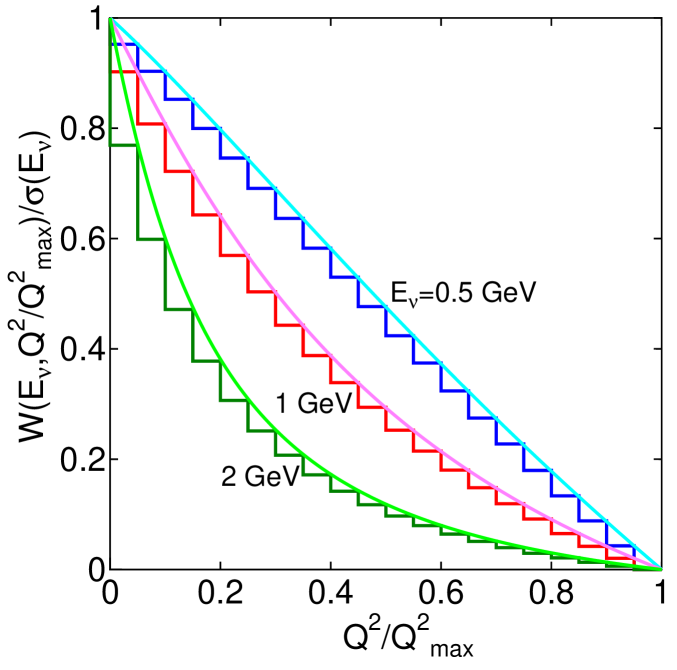
Figure 1: The reproduction of the probability function for QEL cross section. Histograms are sampling results, while the curves concerned are the theoretical ones for given incident energies.

Procedure 2
We obtain $E_{\ell(\bar{\ell})}$ from Eq. (A$\cdot$2) for the given $E_{\nu(\bar{\nu})}$ and $Q^{2}$ obtained as described in Procedure 1.

Procedure 3
We obtain $\cos{\theta_{\rm s}}$, cosine of the the scattering angle of the emitted lepton, for $E_{\ell(\bar{\ell})}$ thus decided in the Procedure 2 from Eq. (A$\cdot$1) in Procedure 2.

Procedure 4
We decide $\phi$, the azimuthal angle of the scattered lepton, which is obtained from

$$\phi=2\pi\xi.$$ (A·5)

where, $\xi$ is a uniform random number on (0, 1).

Procedure 5
The relation between direction cosines of the incident neutrino, $(\ell_{\nu(\bar{\nu})},m_{\nu(\bar{\nu})},n_{\nu(\bar{\nu})})$, and those of the corresponding emitted lepton, $(\ell_{\rm r},m_{\rm r},n_{\rm r})$, for a certain $\theta_{\rm s}$ and $\phi$ is given as

$$\left(\begin{array}[]{c}\ell_{\rm r}\\ m_{\rm r}\\ n_{\rm r}\end{array}\right)=$$ (A·17)

$$\left(\begin{array}[]{ccc}\displaystyle\frac{\ell n}{\sqrt{\ell^{2}+m^{2}}}&-\displaystyle\frac{m}{\sqrt{\ell^{2}+m^{2}}}&\ell_{\nu(\bar{\nu})}\\ \displaystyle\frac{mn}{\sqrt{\ell^{2}+m^{2}}}&\displaystyle\frac{\ell}{\sqrt{\ell^{2}+m^{2}}}&m_{\nu(\bar{\nu})}\\ -\sqrt{\ell^{2}+m^{2}}&0&n_{\nu(\bar{\nu})}\end{array}\right)\times$$

$$\times\left(\begin{array}[]{c}{\rm sin}\theta_{\rm s}{\rm cos}\phi\\ {\rm sin}\theta_{\rm s}{\rm sin}\phi\\ {\rm cos}\theta_{\rm s}\end{array}\right),$$

where $n_{\nu(\bar{\nu})}={\rm cos}\theta_{\nu(\bar{\nu})}$, and $n_{\rm r}={\rm cos}\theta_{\ell}$. Here, $\theta_{\ell}$ is the zenith angle of the emitted lepton.

The Monte Carlo procedure for the determination of $\theta_{\ell}$ of the emitted lepton for the parent (anti-)neutrino with given $\theta_{\nu(\bar{\nu})}$ and $E_{\nu(\bar{\nu})}$ involves the following steps:

We obtain $(\ell_{r},m_{r},n_{r})$ by using Eq. (A·17). The $n_{r}$ is the cosine of the zenith angle of the emitted lepton which should be contrasted with $n_{\nu}$, that of the incident neutrino.
Repeating the procedures 1 to 5 just mentioned above, we obtain the zenith angle distribution of the emitted leptons for a given zenth angle of the incident neutrino with a definite energy.

Appendix B Monte Carlo Procedure to Obtain the Zenith Angle of the Emitted Lepton for a Given Zentith Angle of the Incident Neutrino

The present simulation procedure for a given zenith angle of the incident neutrino starts from the atmospheric neutrino spectrum at the opposite site of the Earth to the underground detector. We define, $N_{\rm int,no-osc}(E_{\nu(\bar{\nu})},t,{\rm cos}\theta_{\nu(\bar{\nu})})$, the interaction neutrino spectrum at the depth $t$ from the underground detector for the case no oscillation in the following way,

$$N_{\rm int,no_{-}osc}(E_{\nu(\bar{\nu})},t,{\cos}\theta_{\nu(\bar{\nu})})=$$

$$N_{\rm sp}(E_{\nu(\bar{\nu})},\cos\theta_{\nu(\bar{\nu})})\times$$

$$\Bigg{(}1-\frac{{\rm d}t}{\lambda_{1}(E_{\nu(\bar{\nu})},t_{1},\rho_{1})}\Bigg{)}\times$$

$$\times\cdots\times\Bigg{(}1-\frac{{\rm d}t}{\lambda_{n}(E_{\nu(\bar{\nu})},t_{n},\rho_{n})}\Bigg{)}.$$

Here, $N_{\rm sp}(E_{\nu(\bar{\nu})},\cos\theta_{\nu(\bar{\nu})})$ is the atmospheric (anti-) neutrino spectrum for the zenith angle at the opposite surface of the Earth. And $\lambda_{i}(E_{\nu(\bar{\nu})},t_{i},\rho_{i})$ denotes the mean free path from QEL for the neutrino (anti-neutrino) with the energy $E_{\nu(\bar{\nu})}$ at the distance, $t_{i}$, from the opposite surface of the Earth, where $\rho_{i}$ is the density.

In the presence of oscillation, neutrino energy spectrum correponding to (B$\cdot$1) is given as,

$$N_{\rm int,osc}(E_{\nu(\bar{\nu})},t,{\cos}\theta_{\nu(\bar{\nu})})$$

$$=N_{\rm int,no_{-}osc}(E_{\nu(\bar{\nu})},\cos\theta_{\nu(\bar{\nu})})\times P(\nu_{\mu}\rightarrow\nu_{\mu})$$

Here, $P(\nu_{\mu}\rightarrow\nu_{\mu})$ is the survival probability of a given flavor, such as $\nu_{\mu}$, and it is given by

$$P(\nu_{\mu}\rightarrow\nu_{\mu})=$$ (B·20)

$$1-sin^{2}2\theta\cdot sin^{2}(1.27\Delta m^{2}L_{\nu}/E_{\nu}),$$

where $sin^{2}2\theta=1.0$ and $\Delta m^{2}=2.4\times 10^{-3}\rm{eV^{2}}$ obtained from Super-Kamiokande Collaboration[1].

The procedures of the Monte Carlo Simulation for the incident neutrino(anti-neutrino) with a given energy, $E_{\nu(\bar{\nu})}$, whose incident direction is expressde by $(l,m,n)$ is as follows.

Procedure A
For the given zenith angle of the incident neutrino, ${\theta_{\nu(\bar{\nu})}}$, we formulate, $N_{\rm pro}(E_{\nu(\bar{\nu})},t,\cos\theta_{\nu(\bar{\nu})}){\rm d}E_{\nu(\bar{\nu})}$, the production function for the neutrino flux to produce leptons at the Kamioka site as follows.

$$N_{\rm pro}(E_{\nu(\bar{\nu})},t,\cos\theta_{\nu(\bar{\nu})}){\rm d}E_{\nu(\bar{\nu})}$$

$$=\sigma_{\ell(\bar{\ell})}(E_{\nu(\bar{\nu})})N_{\rm int}(E_{\nu(\bar{\nu})},t,{\rm cos}\theta_{\nu(\bar{\nu})}){\rm d}E_{\nu(\bar{\nu})},$$

where

$$\displaystyle\sigma_{\ell(\bar{\ell})}(E_{\nu(\bar{\nu})})=\int^{Q_{\rm max}^{2}}_{Q_{\rm min}^{2}}\frac{{\rm d}\sigma_{\ell(\bar{\ell})}(E_{\nu(\bar{\nu})},Q^{2})}{{\rm d}Q^{2}}{\rm d}Q^{2}.$$

Each differential cross section above is given by Eq. (4) in the text. Here, we simply denote the interaction energy spectrum as $N_{\rm int}(E_{\nu(\bar{\nu})},t,{\cos}\theta_{\nu(\bar{\nu})})$ , irrespective of the absence or the presence of oscillation.

Utilizing, $\xi$, a uniform random number on (0,1), we determine $E_{\nu(\bar{\nu})}$, the energy of the incident neutrino by the following sampling procedure,

$$\xi=\int_{E_{\nu(\bar{\nu}),{\rm min}}}^{E_{\nu(\bar{\nu})}}P_{d}(E_{\nu(\bar{\nu})},t,\cos\theta_{\nu(\bar{\nu})}(\bar{\nu})){\rm d}E_{\nu(\bar{\nu})}$$

where

$$P_{d}(E_{\nu(\bar{\nu})},t,\cos{\theta}_{\nu(\bar{\nu})}){\rm d}E_{\nu(\bar{\nu})}$$

$$= \frac{N_{pro}(E_{\nu(\bar{\nu})},t,\cos{\theta}_{\nu(\bar{\nu})}){\rm d}E_{\nu(\bar{\nu})}}{\displaystyle\int_{E_{\nu(\bar{\nu}),{\rm min}}}^{E_{\nu(\bar{\nu}),{\rm max}}}N_{pro}(E_{\nu(\bar{\nu})},t,\cos{\theta}_{\nu(\bar{\nu})}){\rm d}E_{\nu(\bar{\nu})}}.$$

In our Monte Carlo procedure, the reproduction of, $P_{d}(E_{\nu(\bar{\nu})},t,\cos\theta_{\nu(\bar{\nu})}){\rm d}E_{\nu(\bar{\nu})}$, the normalized differential neutrino interaction probability function, is confirmed in the same way as in Eq. (A$\cdot$4).

Procedure B
For the (anti-)neutrino concerned with the energy of $E_{\nu(\bar{\nu})}$, we sample $Q^{2}$ utlizing a uniform random number $\xi$ on (0,1). The Procedure B is exactly the same as Procedure 1 in Appendix A.

Procedure C
We select ${\theta_{\rm s}}$, the scattering angle of the emitted lepton for given $E_{\nu(\bar{\nu})}$ and $Q^{2}$. Procedure C is exactly the same as in the combination of Procedures 2 and 3 in Appendix A.

Procedure D
We randomly sample the azimuthal angle of the charged lepton concerned. The Procedure D is exactly the same as in Procedure 4 in Appendix A.

Procedure E
We decide the direction cosine of the charged lepton concerned. The Procedure E is exactly the same as Procedure 5 in Appendix A.

We repeat Procedures A to E until we reach the desired number of samples.

Appendix C Correlation between the Zenith Angles of the Incident Neutrinos and Those of the Emitted Leptons

Procedure A
By using, $N_{\rm pro}(E_{\nu(\bar{\nu})},t,\cos\theta_{\nu(\bar{\nu})}){\rm d}E_{\nu(\bar{\nu})}$, which is defined in Eq. (LABEL:eqn:b2), we define the spectrum for $\cos\theta_{\nu(\bar{\nu})}$ in the following.

$$I(\cos\theta_{\nu(\bar{\nu})}){\rm d}(\cos\theta_{\nu(\bar{\nu})})=$$

$${\rm d}(\cos\theta_{\nu(\bar{\nu})})\times$$

$$\times\int_{E_{\nu(\bar{\nu}),{\rm min}}}^{E_{\nu(\bar{\nu}),{\rm max}}}N_{\rm pro}(E_{\nu(\bar{\nu})},t,\cos\theta_{\nu(\bar{\nu})}){\rm d}E_{\nu(\bar{\nu})}.$$

using Eq.(C·26) where $\xi$ is a sampled uniform random number on (0,1), we can determine $\cos\theta_{\nu(\bar{\nu})}$

$$\xi=\int_{0}^{\cos\theta_{\nu(\bar{\nu})}}P_{n}(\cos\theta_{\nu(\bar{\nu})}){\rm d}(\cos\theta_{\nu(\bar{\nu})}),$$ (C·26)

where

$$P_{n}(\cos\theta_{\nu(\bar{\nu})})=$$

$$\frac{I(\cos\theta_{\nu(\bar{\nu})})}{\displaystyle\int_{0}^{1}I(\cos\theta_{\nu(\bar{\nu})}){\rm d}(\cos\theta_{\nu(\bar{\nu})})}.$$

Procedure B
For the sampled ${\rm d}(\cos\theta_{\nu(\bar{\nu})})$ in Procedure A, we sample $E_{\nu(\bar{\nu})}$ from Eq.(C·28) by using ${\xi}$, a uniform randum number on (0,1),

$$\xi=\int_{E_{\nu(\bar{\nu}),{\rm min}}}^{E_{\nu(\bar{\nu})}}P_{pro}(E_{\nu(\bar{\nu})},\cos\theta_{\nu(\bar{\nu})}){\rm d}E_{\nu(\bar{\nu})},$$ (C·28)

where

$$P_{pro}(E_{\nu(\bar{\nu})},t,\cos\theta_{\nu(\bar{\nu})}){\rm d}E_{\nu(\bar{\nu})}=$$

$$\frac{N_{\rm pro}(E_{\nu(\bar{\nu})},t,\cos\theta_{\nu(\bar{\nu})}){\rm d}E_{\nu(\bar{\nu})}}{\displaystyle\int_{E_{\nu(\bar{\nu}),{\rm min}}}^{E_{\nu(\bar{\nu}),{\rm max}}}N_{\rm pro}(E_{\nu(\bar{\nu})},t,\cos\theta_{\nu(\bar{\nu})}){\rm d}E_{\nu(\bar{\nu})}}.$$

Procedure C
For the sampled $E_{\nu(\bar{\nu})}$ in Procedure B, we sample $E_{\mu(\bar{\mu})}$ from Eqs. (A·2) and (A·3). From the sampled $E_{\nu(\bar{\nu})}$ and $E_{\mu(\bar{\mu})}$, we determine $\cos{\theta}_{s}$, the scattering angle of the muon uniquely from Eq. (A·1).

Procedure D
We determine, $\phi$, the azimuthal angle of the scattering lepton from Eq. (A·5) by using a uniform randum number ${\xi}$ on (0,1).

Procedure E
We obtain $\cos{\theta}_{\mu(\bar{\mu})}$ from Eq. (A·17). As the result, we obtain a pair of ($\cos\theta_{\nu(\bar{\nu})}$, $\cos{\theta}_{\mu(\bar{\mu})}$) through Procedures A to E. Repeating the Procedures A to E, we finally obtain the correlation between the zenith angle of the incident neutrino and that of the emitted muon.

References

- [1] Ashie,Y. et al., Phys. Rev. D 71 (2005) 112005.
-
[2]
Honda, M., et al., Phys. Rev. D 52 (1996) 4985.
Honda, M., et al., Phys. Rev. D 70 (2004)043008-1. - [3] R.Gandhi, C.Quigg, M.H.Reno, I.Sarcevic, Astropart.Phys.,5 (1996)8
- [4] Renton, P., Electro-weak Interaction, Cambridge University Press (1990). See p. 405.
- [5] Ishitsuka, M, Ph.D thesis, University of Tokyo (2004).