Spectral analysis of a quantum system with a double line singular interaction

Abstract

We consider a non-relativistic quantum particle interacting with a singular potential supported by two parallel straight lines in the plane. We locate the essential spectrum under the hypothesis that the interaction asymptotically approaches a constant value and find conditions which guarantee either the existence of discrete eigenvalues or Hardy-type inequalities. For a class of our models admitting a mirror symmetry, we also establish the existence of embedded eigenvalues and show that they turn into resonances after introducing a small perturbation.

To appear in:  Publ. RIMS, Kyoto University

1 Introduction

The problem we study in this paper belongs to the line of research often called singular perturbations of Schrödinger operators. Let us consider a non-relativistic quantum particle confined to a semiconductor structure $\Sigma\subset\mathbb{R}^{3}$. Suppose the particle has a possibility of tunnelling, therefore the whole $\mathbb{R}^{3}$ forms the configuration space. On the other hand, if the device $\Sigma$ is narrow in a sense we can make an idealization and assume that $\Sigma$ is a set of lower dimension, for example, a surface, a curve or dots in $\mathbb{R}^{3}$. Consequently we come to the model of quantum systems with potential interaction supported by a null set. The interaction can vary on $\Sigma$; let a function $V:\Sigma\to\mathbb{R}$ denote the potential strength. Then the Hamiltonian of such a quantum system can be symbolically written as

$$-\Delta+V\,\delta(\cdot-\Sigma)\,,$$ (1.1)

where $-\Delta$ denotes the Laplace operator in $L^{2}(\mathbb{R}^{3})$ and $\delta$ is the Dirac delta function. In view of singular interactions with translational symmetry, it makes also sense to consider one- and two-dimensional analogues of (1.1).

There are a lot of papers devoted to an analysis of the relation between the geometry of $\Sigma$ and spectral properties of the Hamiltonian with delta interactions of constant strength, cf [6, 11, 12, 13, 15, 16]; we also refer to the monographs [2, 3] with many references. The delta-type potentials supported on infinite curves and surfaces are particularly used for a mathematical modelling of leaky quantum wires and graphs [9, 4].

The simplest, known model belonging to the class described by (1.1) is given by $N$ quantum dots in one dimension, cf [2, Chap. I.3, II.2]. Then $\Sigma:=\{x_{i}\}_{i=0}^{N-1}$ and $V(x_{i}):=-\alpha_{i}\in\mathbb{R}$. For one point interaction (i.e. $N=1$, $\alpha_{0}=:\alpha$) the system possesses one negative eigenvalue $-\alpha^{2}/4$ if, and only if, $\alpha$ is positive. In the case of two point interactions of equal strength (i.e. $N=2$, $\alpha_{0}=\alpha_{1}=:\alpha$) separated by the distance $2a$, there is one negative eigenvalue $\xi_{0}$ if, and only if, $0<\alpha a\leq 1$ or two eigenvalues $\xi_{0}<\xi_{1}$ if, and only if, $\alpha a>1$.

The problem we discuss in this paper can be considered as a generalization of the two quantum dots in two respects. First, our model is two-dimensional, with the set $\Sigma$ being one-dimensional. Second, the generalized geometry enables us to consider potentials $V$ of variable strength. More specifically, we consider the singular set $\Sigma$ composed of two infinite lines

$$\Sigma:=\Sigma_{-}\cup\Sigma_{+}\qquad\mbox{with}\qquad\Sigma_{\pm}:=\mathbb{R}\times\{\pm a\}$$ (1.2)

in $\mathbb{R}^{2}$ and

$$V(x):=\begin{cases}-\alpha+V_{+}(x)&\mbox{if}\quad x\in\Sigma_{+}\,,\\ -\alpha+V_{-}(x)&\mbox{if}\quad x\in\Sigma_{-}\,,\end{cases}$$ (1.3)

with $V_{\pm}:\Sigma_{\pm}\to\mathbb{R}$ and $\alpha>0$. In the physical setting described above, the negative part $-\alpha$ of $V$ models the confinement of the particle to $\Sigma$, while $V_{\pm}$ can be thought as a perturbation.

Our first aim is to find a self-adjoint realization in $L^{2}(\mathbb{R}^{2})$ of (1.1) with (1.2)–(1.3). We will do this by means of a form-sum method and the resulting operator will be called $H_{\alpha,V_{+},V_{-}}$. Note that the delta potential in our model does not vanish at infinity even if $V_{\pm}$ do (just because $\alpha$ is assumed to be positive). This means that we may expect that the essential spectrum of $H_{\alpha,V_{+},V_{-}}$ will differ from the spectrum of the free Hamiltonian in $\mathbb{R}^{2}$. In our setting, the role of the unperturbed Hamiltonian is played by $H_{\alpha,0,0}$.

For the unperturbed Hamiltonian, the translational symmetry allows us to decompose the operator as follows

$$H_{\alpha,0,0}\simeq(-\Delta^{\mathbb{R}})\otimes 1+1\otimes(-\Delta_{\alpha}^{\mathbb{R}})\qquad\mbox{on}\qquad L^{2}(\mathbb{R})\otimes L^{2}(\mathbb{R})\,,$$ (1.4)

where $-\Delta^{\mathbb{R}}$ is the free one-dimensional Hamiltonian and $-\Delta_{\alpha}^{\mathbb{R}}$ governs the aforementioned one-dimensional system with two points interactions. The non-negative semi-axis constitutes the spectrum of $-\Delta^{\mathbb{R}}$. On the other hand, as was already mentioned, the spectrum of $-\Delta_{\alpha}^{\mathbb{R}}$ takes the form

$$\sigma(-\Delta_{\alpha}^{\mathbb{R}})=\sigma_{\mathrm{disc}}(-\Delta_{\alpha}^{\mathbb{R}})\cup[0,\infty)\,,$$

with the negative eigenvalues (cf Lemma 2.3 and Figure 1)

$$\sigma_{\mathrm{disc}}(-\Delta_{\alpha}^{\mathbb{R}})=\begin{cases}\{\xi_{0}\}&\mbox{if}\quad 0<\alpha a\leq 1\,,\\ \{\xi_{0},\xi_{1}\}&\mbox{if}\quad\alpha a>1\,,\end{cases}$$

(the discrete spectrum is empty in the other situations, which is excluded here by the assumption $\alpha>0$). Recalling the ordering $\xi_{0}<\xi_{1}$ (if the latter exists), we conclude (irrespectively of the value of $\alpha a$) with

$$\sigma(H_{\alpha,0,0})=\sigma_{\mathrm{ess}}(H_{\alpha,0,0})=[\xi_{0},\infty)\,.$$ (1.5)

The main results of the paper can be formulated as follows.
$\bullet$ Definition of the Hamiltonian and its resolvent. The definition of the Hamiltonian $H_{\alpha,V_{+},V_{-}}$ by means of the form-sum method is given in Section 2. We also derive a Krein-like formula for the resolvent of $H_{\alpha,V_{+},V_{-}}$ as a useful tool for further discussion.
$\bullet$ Essential spectrum. In Section 3 we find a weak condition preserving the stability of the essential spectrum of $H_{\alpha,V_{+},V_{-}}$ with respect to $H_{\alpha,0,0}$. We show that if $V_{\pm}$ vanish at infinity then

$$\sigma_{\mathrm{ess}}(H_{\alpha,V_{+},V_{-}})=\sigma_{\mathrm{ess}}(H_{\alpha,0,0})=[\xi_{0},\infty)\,.$$ (1.6)

The strategy of our proof is as follows. Using a Neumann bracketing argument together with minimax principle, we get $\inf\sigma_{\mathrm{ess}}(H_{\alpha,V_{+},V_{-}})\geq\xi_{0}$. The opposite inclusion $\sigma_{\mathrm{ess}}(H_{\alpha,V_{+},V_{-}})\supseteq[\xi_{0},\infty)$ is obtained by means of the Weyl criterion adapted to sesquilinear forms.
$\bullet$ Discrete and embedded eigenvalues. The point spectrum is investigated in Section 4. We show that the bottom of the spectrum of $H_{\alpha,V_{+},V_{-}}$ starts below $\xi_{0}$ provided that the sum $V_{+}+V_{-}$ is negative in an integral sense. Assuming additionally that $V_{\pm}$ vanish at the infinity and combining this with the previous result on the essential spectrum, we therefore obtain a non-trivial property

$$\sigma_{\mathrm{disc}}(H_{\alpha,V_{+},V_{-}})\neq\emptyset\,.$$ (1.7)

The proof is based on finding a suitable test function in the variational definition of the spectral threshold. We also find conditions which guarantee the existence of embedded eigenvalues in the system with mirror symmetry, i.e. $V_{+}=V_{-}$.
$\bullet$ Hardy inequalities. The case of repulsive singular potentials, i.e. $V_{\pm}\geq 0$, is studied in Section 5. In order to quantify how strong the repulsive character of singular potential is, we derive Hardy-type inequalities

$$H_{\alpha,V_{+},V_{-}}-\xi_{0}\,\geq\,\varrho$$ (1.8)

in the form sense, where $\varrho:\mathbb{R}\to[0,\infty)$ is not identically zero. The functional inequality (1.8) is useful in the study of spectral stability of $H_{\alpha,V_{+},V_{-}}$; indeed, it determines a class of potentials which can be added to our system without producing any spectrum below $\xi_{0}$.
$\bullet$ Resonances. Finally, in Section 6 we show that breaking the mirror symmetry by introducing a “perturbant” function $V_{p}$ on one of the line, for example

$$V_{+}=V_{0}+\epsilon V_{p}\,,\qquad V_{-}=V_{0}\,,$$

leads to resonances. These resonances are localized near the original embedded eigenvalues $\nu_{k}$ appearing when $\epsilon=0$. Precisely, they are determined by poles of the resolvent which take the form

$$z_{k}=\nu_{k}+\mu_{k}(\epsilon)+i\upsilon_{k}(\epsilon)\,,$$

where $\mu_{k}(\epsilon)=a_{k}\epsilon+\mathcal{O}(\epsilon^{2})$ with $a_{k}$ corresponding to the first order perturbation term and $\upsilon_{k}(\epsilon)=b_{k}\mathcal{O}(\epsilon^{2})$ where $b_{k}<0$ establishes the Fermi golden rule.

Let us conclude this introductory section by pointing out some special notation frequently used throughout the paper. We abbreviate $L^{2}:=L^{2}(\mathbb{R}^{2})$ and $L_{\pm}^{2}:=L^{2}(\mathbb{R}\times\{\pm a\})$. We also shortly write $W^{n,2}:=W^{n,2}(\mathbb{R}^{2})$ for the corresponding Sobolev spaces. The inner product and norm in $L^{2}$ is denoted by $(\cdot,\cdot)$ and $\|\cdot\|$, respectively. Given a self-adjoint operator $H$, the symbols $\sigma_{\iota}(H)$ with $\iota\in\{\mathrm{ess},\mathrm{ac},\mathrm{sc},\mathrm{p},\mathrm{disc}\}$ denote, respectively, the essential, absolutely continuous, singularly continuous, point and discrete spectrum of $H$. We use the symbol $1$ to denote identity operators acting in various Hilbert spaces used in the paper.

2 The Hamiltonian and its resolvent

Let $V_{+}$ and $V_{-}$ be two real-valued functions from $L^{\infty}(\mathbb{R})$. Given a positive number $a$, we denote by the same symbols the functions $V_{+}\otimes 1$ and $V_{-}\otimes 1$ on $\mathbb{R}\times\{+a\}$ and $\mathbb{R}\times\{-a\}$, respectively. Finally, let $\alpha$ be a positive constant.

2.1 The self-adjoint realization of the Hamiltonian

Let us consider the following quadratic form

$$\mathcal{E}_{\alpha,V_{+},V_{-}}[\psi] :=\int_{\mathbb{R}^{2}}|\nabla\psi|^{2}+\int_{\mathbb{R}\times\{+a\}}(V_{+}-\alpha)\,|I_{+}\psi|^{2}+\int_{\mathbb{R}\times\{-a\}}(V_{-}-\alpha)\,|I_{-}\psi|^{2}\,,$$

$$\mathfrak{D}(\mathcal{E}_{\alpha,V_{+},V_{-}}) :=W^{1,2}\,.$$

Here $I_{\pm}$ are the trace operators associated with the Sobolev embedding $W^{1,2}\hookrightarrow L^{2}_{\pm}$. The corresponding sesquilinear form will be denoted by $\mathcal{E}_{\alpha,V_{+},V_{-}}(\cdot,\cdot)$.

The form $\mathcal{E}_{\alpha,V_{+},V_{-}}$ is clearly densely defined and symmetric. Moreover, the boundary integrals can be shown to be a relatively bounded perturbation of the form $\mathcal{E}_{0,0,0}$ with the relative bound less than $1$. This is a consequence of the boundedness of $V_{\pm}$ and the following result.

Lemma 2.1.

For every $\psi\in W^{1,2}$ and $\epsilon\in(0,1)$, we have

$$\|I_{\pm}\psi\|_{L_{\pm}^{2}}^{2}\leq\frac{1}{\epsilon}\,\|\psi\|_{L^{2}}^{2}+\epsilon\,\|\partial_{2}\psi\|_{L^{2}}^{2}\,.$$ (2.9)

Proof.

For every $\epsilon\in(0,1)$ and $\psi\in C_{0}^{\infty}(\mathbb{R}^{2})$, we have the bound

$$|\psi(x_{1},\pm a)|^{2} =\int_{-\infty}^{\pm a}\partial_{2}|\psi|^{2}(x_{1},x_{2})\,dx_{2}=2\,\Re\int_{-\infty}^{\pm a}\overline{\psi(x_{1},x_{2})}\,\partial_{2}\psi(x_{1},x_{2})\,dx_{2}$$

$$\leq\frac{1}{\epsilon}\int_{\mathbb{R}}|\psi(x_{1},x_{2})|^{2}\,dx_{2}+\epsilon\int_{\mathbb{R}}|\partial_{2}\psi(x_{1},x_{2})|^{2}\,dx_{2}\,.$$

Integrating over $x_{1}$, we therefore get (2.9) for $\psi\in C_{0}^{\infty}(\mathbb{R}^{2})$. By density, the obtained inequality extends to $W^{1,2}$. ∎

Remark 2.2 (Relation to the generalized Kato class).

Inequality (2.9) represents a quantification of the embedding $W^{1,2}\hookrightarrow L_{\pm}^{2}$. If the support of the singular potential has a more complicated geometry we can derive a generalization of (2.9). Consider a Radon measure $\mu$ on $\mathbb{R}^{2}$ with a support on a $C^{1}$ curve (finite or infinite) without self-intersections and “near-self-intersections” (see [5, Sec. 4] for precise assumptions). Such a measure belongs to the generalized Kato class (cf [5, Thm. 4.1]) and, consequently, for any $a>0$ there exists $b>0$ such that

$$\int_{\mathbb{R}^{2}}|\psi|^{2}\,\mathrm{d}\mu\leq b\,\|\psi\|_{L^{2}}^{2}+a\,\|\nabla\psi\|_{L^{2}}^{2}$$

for every $\psi\in W^{1,2}$.

Since $\mathcal{E}_{0,0,0}$ is clearly closed and non-negative (it is in fact associated with the free Hamiltonian in $\mathbb{R}^{2}$), it follows by the KLMN theorem [25, Thm. X.17] with help of Lemma 2.1 that $\mathcal{E}_{\alpha,V_{+},V_{-}}$ is closed and bounded from below. Consequently, there exists a unique bounded-from-below self-adjoint operator $H_{\alpha,V_{+},V_{-}}$ in $L^{2}$ which is associated with $\mathcal{E}_{\alpha,V_{+},V_{-}}$. (Notice that the sign of $\alpha$ plays no role in the definition of $H_{\alpha,V_{+},V_{-}}$.)

Finally, let us note that $H_{\alpha,V_{+},V_{-}}$ is indeed a natural realization of the formal expression (1.1) with (1.2)–(1.3). As a matter of fact, our form $\mathcal{E}_{\alpha,V_{+},V_{-}}$ represents a closed extension of the form associated with the expression (1.1) initially considered as acting on smooth functions rapidly decaying at the infinity of $\mathbb{R}^{2}$.

2.2 The transverse Hamiltonian

Recall the decomposition (1.4) for the unperturbed Hamiltonian $H_{\alpha,0,0}$. Here the “transverse” operator $-\Delta_{\alpha}^{\mathbb{R}}$ is associated with the form

$$\varepsilon_{\alpha}[\phi]:=\int_{\mathbb{R}}|\phi^{\prime}|^{2}-\alpha\,|\phi(+a)|^{2}-\alpha\,|\phi(-a)|^{2}\,,\qquad\mathfrak{D}(\varepsilon_{\alpha}):=W^{1,2}(\mathbb{R})\,.$$

Note that the boundary values have a good meaning in view of the embedding $W^{1,2}(\mathbb{R})\hookrightarrow C^{0}(\mathbb{R})$. It is easy to verify that $\mathfrak{D}(-\Delta_{\alpha}^{\mathbb{R}})$ consists of functions $\psi\in W^{1,2}(\mathbb{R})\cap W^{2,2}(\mathbb{R}\setminus\{-a,+a\})$ satisfying the interface conditions

$$\psi^{\prime}(\pm a+0)-\psi^{\prime}(\pm a-0)=-\alpha\psi(\pm a)\,,$$ (2.10)

where $\psi^{\prime}(a\pm 0):=\lim_{\epsilon\to 0^{+}}\psi^{\prime}(a\pm\epsilon)$, and that $-\Delta_{\alpha}^{\mathbb{R}}\psi=-\psi^{\prime\prime}$ on $\mathbb{R}\setminus\{-a,+a\}$. An alternative way of introducing $-\Delta_{\alpha}^{\mathbb{R}}$ is via the extension theory [2, Chap. II.2].

Due to [2, Thm. 2.1.3], we have $\sigma_{\mathrm{ess}}(-\Delta_{\alpha}^{\mathbb{R}})=\sigma_{\mathrm{ac}}(-\Delta_{\alpha}^{\mathbb{R}})=[0,\infty)$. The structure of discrete spectrum depends on the strength of $\alpha a$.

Lemma 2.3.

Operator $-\Delta_{\alpha}^{\mathbb{R}}$ has exactly two negative eigenvalues if $\alpha a>1$ and exactly one negative eigenvalue if $0<\alpha a\leq 1$.

Proof.

Let $\kappa>0$. Solving the eigenvalue problem $-\psi^{\prime\prime}=-\kappa^{2}\psi$ on $\mathbb{R}\setminus\{-a,+a\}$ in terms of exponential functions decaying at infinity and using the continuity of $\psi$ and (2.10), it is straightforward to see that the algebraic equation

$$\frac{\alpha^{2}}{4}\,\mathrm{e}^{-4\kappa a}=\left(\kappa-\frac{\alpha}{2}\right)^{2}$$ (2.11)

represents a sufficient and necessary condition for $-\kappa^{2}\in\sigma_{\mathrm{p}}(-\Delta_{\alpha}^{\mathbb{R}})$. (Alternatively, one could use directly [2, Eq. (2.1.33)].) Equation (2.11) is equivalent to $g_{1}(\kappa)-g_{2}(\kappa)=0$ with

$$g_{1}(\kappa):=\frac{\alpha}{2}\mathrm{e}^{-2\kappa a}\,\quad\mathrm{and}\quad g_{2}(\kappa):=\left|\kappa-\frac{\alpha}{2}\right|\,.$$ (2.12)

Since the exponential function $g_{1}$ is positive monotonously decreasing and $g_{2}$ is monotonously increasing for $\kappa\in(\alpha/2\,,\infty)$ with $g_{2}(\alpha/2)=0$, there exists exactly one solution $\kappa_{0}>\alpha/2$ of (2.11) for any $\alpha>0$. Since $g_{1}$ is strictly convex, $g_{1}(0)=g_{2}(0)$ and the graph of $g_{2}$ is a straight line for $\kappa\in(0,\alpha/2)$ with $g_{2}^{\prime}(0)=-1$, the existence of another (at most one) solution $\kappa_{1}\in(0,\alpha/2)$ is determined by the derivative of $g_{1}$ at $0$. Obviously, $g_{1}^{\prime}(0)\geq-1$ if, and only if, $\alpha a\leq 1$. We set $\xi_{0}:=-\kappa_{0}^{2}$ and $\xi_{1}:=-\kappa_{1}^{2}$ (if the latter exists). ∎

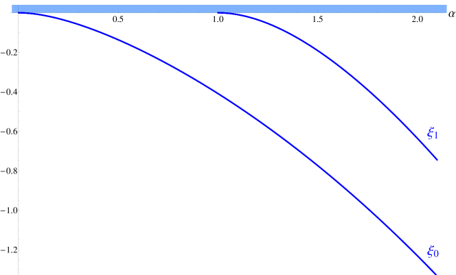
Figure 1: Emergence of the discrete eigenvalues $\xi_{0}$, $\xi_{1}$ from the essential spectrum as $\alpha$ increases for $a=1$.

We refer to Figure 1 for the dependence of the discrete spectrum on $\alpha a$. The eigenfunctions corresponding to $\xi_{0}$ and $\xi_{1}$ will be denoted by $\phi_{0}$ and $\phi_{1}$, respectively. For notational purposes, it will become convenient to introduce the index set

$$\mathcal{N}:=\begin{cases}\{0\}&\mbox{if}\quad\alpha a\leq 1\,,\\ \{0\,,1\}&\mbox{if}\quad\alpha a>1\,.\end{cases}$$ (2.13)

Due to the symmetry of the system, $\phi_{0}$ is even and $\phi_{1}$ is odd. Moreover, $\phi_{0}$ can be chosen positive, cf [2, Thm. 2.1.3].

2.3 A lower-bound Hamiltonian

In this subsection we derive an auxiliary result we shall use several times later on. It is based on an idea used in a similar context in [17].

Taking into account the structure of $\mathcal{E}_{\alpha,V_{+},V_{-}}$, let us define

$$\tilde{\lambda}(v_{+},v_{-}):=\inf_{\phi\in W^{1,2}(\mathbb{R})\setminus\{0\}}\frac{\varepsilon_{\alpha}[\phi]+v_{+}|\phi(+a)|^{2}+v_{-}|\phi(-a)|^{2}}{\|\phi\|_{L^{2}(\mathbb{R})}^{2}}-\xi_{0}$$ (2.14)

for any real constants $v_{+}$ and $v_{-}$. The number $\tilde{\lambda}(v_{+},v_{-})$ is the lowest eigenvalue of the operator (1.1) on $L^{2}(\mathbb{R})$ shifted by $\xi_{0}$, subject to two point interactions of strength $v_{+}-\alpha$ and $v_{-}-\alpha$ separated by the distance $2a$.

It is clear that $\tilde{\lambda}(v_{+},v_{-})$ is a continuous and monotonous non-decreasing function of both $v_{+}$ and $v_{-}$. The symmetry relation $\tilde{\lambda}(v_{+},v_{-})=\tilde{\lambda}(v_{-},v_{+})$ holds true. Assume that both $v_{\pm}$ are non-negative. Then by the variational definition of $\xi_{0}$, we have $\tilde{\lambda}(v_{+},v_{-})\geq 0$ and $\tilde{\lambda}(0,0)=0$. For our purposes, it is important to point out that $\tilde{\lambda}(v_{+},v_{-})$ is positive whenever at least one of the arguments is. Indeed, if $\tilde{\lambda}(v_{+},v_{-})=0$ and $v_{+}>0$ or $v_{-}>0$, then we get from (2.14) that the minimum is achieved by the eigenfunction $\phi_{0}$ of $-\Delta_{\alpha}^{\mathbb{R}}$ corresponding to $\xi_{0}$ and that $\phi_{0}(a)=0$ or $\phi_{0}(-a)=0$. Since $\phi_{0}$ is positive the latter leads to the contradiction.

If $V_{+}$ and $V_{-}$ are real-valued functions, then $\tilde{\lambda}$ gives rise to a function $\lambda:\mathbb{R}^{2}\to\mathbb{R}$ via setting

$$\lambda(x):=\tilde{\lambda}\big{(}V_{+}(x_{1}),V_{-}(x_{1})\big{)}\,.$$ (2.15)

It follows from the properties of $\tilde{\lambda}$ that if $V_{\pm}$ are non-negative and $V_{-}$ or $V_{+}$ is non-trivial (i.e., non-zero on a measurable set of positive Lebesgue measure), then $\lambda$ is a non-trivial non-negative function.

In any case, using Fubini’s theorem, we get a fundamental lower bound for our form $\mathcal{E}_{\alpha,V_{+},V_{-}}$.

Lemma 2.4.

For every $\psi\in W^{1,2}$, we have

$$\mathcal{E}_{\alpha,V_{+},V_{-}}[\psi]-\xi_{0}\,\|\psi\|_{L^{2}}^{2}\geq\int_{\mathbb{R}^{2}}|\partial_{1}\psi|^{2}+\int_{\mathbb{R}^{2}}\lambda\,|\psi|^{2}\,.$$ (2.16)

The above result shows that $H_{\alpha,V_{+},V_{-}}-\xi_{0}$ is bounded from below by the one-dimensional Schrödinger operator

$$(-\Delta^{\mathbb{R}}+\lambda)\otimes 1\qquad\mbox{on}\qquad L^{2}(\mathbb{R})\otimes L^{2}(\mathbb{R})\,.$$

2.4 The Krein-like resolvent formula

The first auxiliary step is to reconstruct the resolvent of the unperturbed Hamiltonian, i.e. $R_{\alpha}(z):=(H_{\alpha,0,0}-z)^{-1}$ for $z\in\mathbb{C}\setminus[\xi_{0},\infty)$. Once we have $R_{\alpha}(z)$ we introduce potentials $V_{\pm}$ and build up the Krein-like resolvent of $H_{\alpha,V_{+},V_{-}}$ as a perturbation of $R_{\alpha}(\cdot)$. For this aim we will follow the treatment derived by Posilicano [22].

2.4.1 The resolvent of the unperturbed Hamiltonian

As above, $\xi_{j}$, with $j\in\mathcal{N}$, stand for the discrete eigenvalues of $-\Delta^{\mathbb{R}}_{\alpha}$ and $\phi_{j}$ denote the corresponding eigenfunctions. Recall that the essential spectrum of $-\Delta^{\mathbb{R}}_{\alpha}$ is purely absolutely continuous. Let $E_{\alpha}^{\mathbb{R}}(\cdot)$ stand for the spectral resolution of $-\Delta^{\mathbb{R}}_{\alpha}$ corresponding to the continuous spectrum and $P_{\alpha,j}$, with $j\in\mathcal{N}$, denote the eigen-projectors $P_{\alpha,j}=\phi_{j}(\phi_{j},\cdot)$. Analogously, $E^{\mathbb{R}}(\cdot)$ denotes the spectral resolution of $-\Delta^{\mathbb{R}}$. Using (1.4), one gets

$$R_{\alpha}(z)=\sum_{j\in\mathcal{N}}\int_{\mathbb{R}_{+}}(\beta+\xi_{j}-z)^{-1}\mathrm{d}E^{\mathbb{R}}(\beta)\otimes P_{\alpha,j}+\int_{\mathbb{R}^{2}_{+}}(\beta+\beta^{\prime}-z)^{-1}\mathrm{d}E^{\mathbb{R}}(\beta)\otimes\mathrm{d}E^{\mathbb{R}}_{\alpha}(\beta^{\prime})\,,$$

where $z\in\mathbb{C}\setminus[\xi_{0}\,,\infty)$. This implies the decomposition

$$R_{\alpha}(z)=R_{\alpha}^{d}(z)+R_{\alpha}^{c}(z)\,,$$

where $R_{\alpha}^{\iota}(z)$, with $\iota\in\{d,c\}$, act on a separated variable function $f(x)=f_{1}(x_{1})f_{2}(x_{2})$ as

$$R_{\alpha}^{d}(z)f(x) =\sum_{j\in\mathcal{N}}\frac{1}{\sqrt{2\pi}}\int_{\mathbb{R}}\mathrm{d}p_{1}\,\frac{\widehat{f}_{1}(p_{1})\mathrm{e}^{ip_{1}x_{1}}}{p_{1}^{2}+\xi_{j}-z}\phi_{j}(x_{2})(\phi_{j},f_{2})_{L^{2}(\mathbb{R})}\,,$$

$$R_{\alpha}^{c}(z)f =\int_{\mathbb{R}^{2}_{+}}\frac{1}{\beta+\beta^{\prime}-z}\mathrm{d}E^{\mathbb{R}}(\beta)f_{1}\otimes\mathrm{d}E_{\alpha}^{\mathbb{R}}(\beta^{\prime})f_{2}\,,$$

with $\widehat{f_{1}}$ denoting the Fourier transform of $f_{1}$. Set $\tau_{j}^{2}(z):=z-\xi_{j}$. In the following we assume that $z$ is taken from the first sheet of the domain of function $z\mapsto\tau_{j}(z)$, i.e. $\Im\tau_{j}(z)>0$.

Using the standard representation of the Green function of the one-dimensional Laplace operator

$$(-\Delta^{\mathbb{R}}-k^{2})^{-1}(x_{1},y_{1})=\frac{1}{2\pi}\int_{\mathbb{R}}\frac{\mathrm{e}^{ip(x_{1}-y_{1})}}{p^{2}-k^{2}}\,\mathrm{d}p=\frac{i}{2}\frac{\mathrm{e}^{ik|x_{1}-y_{1}|}}{k}\,$$

we conclude that $R_{\alpha}^{d}(z):=\sum_{j\in\mathcal{N}}R_{\alpha}^{j,d}(z)$ where $R_{\alpha}^{j,d}(z)$ are integral operators with the kernels

$$G_{\alpha}^{j,d}(z;x,y)= \frac{i}{2}\frac{\mathrm{e}^{i\tau_{j}(z)|x_{1}-y_{1}|}}{\tau_{j}(z)}\phi_{j}(x_{2})\overline{\phi_{j}(y_{2})}\,.$$ (2.17)

Moreover

$$R^{c}_{\alpha}(z)f=\frac{i}{2}\int_{\mathbb{R}^{2}}\int_{\mathbb{R}}\frac{\mathrm{e}^{i\tau(p,z)|x_{1}-y_{1}|}}{\tau(p,z)}\psi(p\,,x_{2})\overline{\psi(p\,,y_{2})}f_{1}(y_{1})f_{2}(y_{2})\,\mathrm{d}y_{1}\mathrm{d}y_{2}\mathrm{d}p\,,$$ (2.18)

where $\tau^{2}(p,z)=z-p^{2}$, $\Im\tau(p,z)>0$ and $\psi(p\,,x_{2})$ stand for the generalized eigenfunctions of $-\Delta^{\mathbb{R}}_{\alpha}$ discussed in [2, Chap. II.2.4]. To be fully specific $\psi(p\,,x_{2})$ can be obtained from Eq. (2.4.1) of [2, Chap. II] multiplying it by the factor $\frac{1}{2\pi}$, see also [2, Appendix E], Eq. (E.5).

The resolvent of $H_{\alpha,0,0}$ can be written also in a Krein-like form. We start with the resolvent of the free system $R_{0}(z)=(H_{0,0,0}-z)^{-1}$, $z\in\mathbb{C}\setminus[0,\infty)$. By means of the embeddings $I_{\pm}\,:\,W^{1,2}\hookrightarrow L_{\pm}^{2}$ and theirs adjoints $I^{\ast}_{\pm}\,:\,L_{\pm}^{2}\hookrightarrow W^{-1,2}$, we define

$$\hat{R}_{0,\pm}(z):=I_{\pm}R_{0}(z)\,:L^{2}\to L_{\pm}^{2}\,,\quad\check{R}_{0,\pm}(z):=R_{0}(z)I^{\ast}_{\pm}\,:L_{\pm}^{2}\to L^{2}.$$

Finally, the “bilateral” embeddings take the forms

$$\mathrm{R}_{0,ij}(z):=I_{i}R_{0}(z)I^{\ast}_{j}\,:\,L^{2}(\mathbb{R}\times\{ja\})\to L^{2}(\mathbb{R}\times\{ia\})\,,\qquad i,j\in\{+\,,-\}\,.$$

Let $\Gamma_{0,\alpha}(z)$ denote the operator-valued matrix acting in $L^{2}_{+}\oplus L^{2}_{-}$ and taking the form

$$\Gamma_{0,\alpha}(z):=\begin{pmatrix}-\alpha^{-1}\,,&0\\ 0\,,&-\alpha^{-1}\end{pmatrix}+\begin{pmatrix}\mathrm{R}_{0,++}(z)\,,&\mathrm{R}_{0,+-}(z)\\ \mathrm{R}_{0,-+}(z)\,,&\mathrm{R}_{0,--}(z)\end{pmatrix}\,.$$

Note that the continuity of $I_{i}\,:\,W^{1,2}\hookrightarrow L^{2}_{i}$, $i\in\{+\,,-\}$ implies the continuity of the adjoint embedding $I_{i}^{\ast}\,:\,L^{2}_{i}\hookrightarrow W^{-1,2}$. Therefore

$$\mathrm{Ran}\,\check{R}_{0,i}(z)\subset W^{1,2}\,.$$ (2.19)

Moreover, since $\mathrm{Ran}\,I_{i}^{\ast}\cap L^{2}=\{0\}$, we obtain

$$\mathrm{Ran}\,\check{R}_{0,i}(z)\cap W^{2,2}=\{0\}\,.$$ (2.20)

Theorem 2.5.

Let $z\in\mathbb{C}\setminus[\xi_{0},\infty)$ be such that the operator $\Gamma_{0,\alpha}(z)$ is invertible with bounded inverse. Then the resolvent $R_{\alpha}(z)$ is given by

$$R_{\alpha}(z)=R_{0}(z)-\sum_{i,j\in\{+,-\}}\check{R}_{0,i}(z)\Gamma_{0,\alpha}(z)_{ij}^{-1}\hat{R}_{0,j}(z)\,,$$ (2.21)

where $\Gamma_{0,\alpha}(z)_{ij}^{-1}$ are the matrix elements of the inverse of $\Gamma_{0,\alpha}(z)$.

Proof.

In view of (2.19), operator $R_{\alpha}(z)$ defined by (2.21) satisfies $\mathrm{Ran}\,R_{\alpha}(z)\subset W^{1,2}$. Assume $\psi\in W^{1,2}$ and $\phi\in L^{2}$. Using $\mathcal{E}_{0,0,0}(\psi,R_{0}(z)\phi)-z(\psi,R_{0}(z)\phi)=(\psi,\phi)$, we get

$$\mathcal{E}_{\alpha,0,0}\big{(}\psi,R_{\alpha}(z)\phi\big{)}-z\big{(}\psi,R_{\alpha}(z)\phi\big{)}=(\psi,\phi)$$

$$-\sum_{i\in\{+,-\}}\alpha\big{(}\psi,\hat{R}_{0,i}(z)\phi\big{)}_{L^{2}_{i}}-\sum_{i,j\in\{+,-\}}\big{(}\psi,\Gamma_{0,\alpha}(z)_{ij}^{-1}\hat{R}_{0,j}(z)\phi\big{)}_{L^{2}_{i}}$$

$$+\sum_{i,j,k\in\{+,-\}}\alpha\big{(}\psi,\mathrm{R}_{0,ij}(z)\Gamma_{0,\alpha}(z)_{jk}^{-1}\hat{R}_{0,k}(z)\phi\big{)}_{L^{2}_{i}}\,,$$

where we use the embedding $W^{1,2}\hookrightarrow L_{i}^{2}$ for $\psi$ in all expressions with scalar product in $L^{2}_{i}$. Applying the identity

$$\big{(}\psi,\hat{R}_{0,i}(z)\phi\big{)}_{L^{2}_{i}}=\sum_{j,k\in\{+,-\}}\big{(}\psi,\Gamma_{0,\alpha}(z)_{ik}\Gamma_{0,\alpha}(z)_{kj}^{-1}\hat{R}_{0,j}(z)\phi\big{)}_{L^{2}_{i}}$$

and using the explicit form of $\Gamma_{0,\alpha}(z)_{ij}$, one obtains

$$\mathcal{E}_{\alpha,0,0}\big{(}\psi,R_{\alpha}(z)\phi\big{)}-z\big{(}\psi,R_{\alpha}(z)\phi\big{)}=(\psi,\phi)\,.$$ (2.22)

Moreover, note that $R_{\alpha}(z)$ is invertible. Indeed, employing (2.21) and (2.20) we conclude that any $f\in\mathrm{Ran}\,R_{\alpha}(z)$ has a form of direct sum $f=f_{1}\dot{+}f_{2}$ where $f_{1}\in\mathrm{Ran}\,R_{0}(z)$ and $f_{2}\in W^{1,2}\setminus W^{2,2}$. This implies $\mathrm{Ker}\,R_{\alpha}=\{0\}$ and together with (2.22) completes the proof. ∎

2.4.2 The Krein-like formula for the resolvent of $H_{\alpha,V_{+},V_{-}}$

Relying on (2.21) and (2.19), we can determine the analogous embeddings operators as in the previous section but now instead of $R_{0}(z)$ we consider $R_{\alpha}(z)$. Namely, define $\hat{R}_{\alpha,\pm}(z):=I_{\pm}R_{\alpha}(z)\,:L^{2}\to L_{\pm}^{2}\,$, $\check{R}_{\alpha,\pm}(z):=R_{\alpha}(z)I^{\ast}_{\pm}\,:\,L_{\pm}^{2}\to L^{2}$ and $\mathrm{R}_{\alpha,ij}(z):=I_{i}R_{\alpha}(z)I^{\ast}_{j}\,:\,L^{2}_{j}\to L^{2}_{i}$ where $i,j\in\{+\,,-\}$.

For any bounded function $V$, let us set $V^{1/2}:=\mathop{\mathrm{sgn}}\nolimits(V)|V|^{1/2}$. Define the operator-valued matrix

$$B(z):=\begin{pmatrix}|V_{+}|^{1/2}\mathrm{R}_{\alpha,++}(z)V_{+}^{1/2}\,,&|V_{+}|^{1/2}\mathrm{R}_{\alpha,+-}(z)V_{-}^{1/2}\\ |V_{-}|^{1/2}\mathrm{R}_{\alpha,-+}(z)V_{+}^{1/2}\,,&|V_{-}|^{1/2}\mathrm{R}_{\alpha,--}(z)V_{-}^{1/2}\end{pmatrix}$$

acting on $L_{+}^{2}\oplus L_{-}^{2}$.

Theorem 2.6.

Let $z\in\mathbb{C}\setminus\sigma(H_{\alpha,V_{+},V_{-}})$ be such that the operator $1+B(z)$ is invertible with bounded inverse. Then

$$R_{\alpha,V_{+},V_{-}}(z)=R_{\alpha}(z)-\sum_{i,j\in\{+,-\}}\check{R}_{\alpha,i}(z)V_{i}^{1/2}[1+B(z)]_{ij}^{-1}|V_{j}|^{1/2}\hat{R}_{\alpha,j}(z)\,$$ (2.23)

determines the resolvent of $H_{\alpha,V_{+},V_{-}}$; the notions $[1+B(z)]_{ij}^{-1}$ stand for the operator valued matrix elements of $[1+B(z)]^{-1}$.

Proof.

Combining (2.21) and (2.19) and using the definition of $R_{\alpha,V_{+},V_{-}}(z)$ given by (2.23) we have $\mathrm{Ran}\,\check{R}_{\alpha,i}(z)\subset W^{1,2}$ and consequently $\mathrm{Ran}\,R_{\alpha,V_{+},V_{-}}(z)\subset W^{1,2}$.

Denote $\Upsilon(z)_{ij}:=[1+B(z)]_{ij}^{-1}$ and assume $\psi\in W^{1,2}$ and $\phi\in L^{2}$. Employing the identity $\mathcal{E}_{\alpha,0,0}(\psi,R_{\alpha}(z)\phi)-z(\psi,R_{\alpha}(z)\phi)=(\psi,\phi)$ we get

$$\mathcal{E}_{\alpha,V_{+},V_{-}}\big{(}\psi,R_{\alpha,V_{+},V_{-}}(z)\phi\big{)}-z\big{(}\psi,R_{\alpha,V_{+},V_{-}}(z)\phi\big{)}=(\psi,\phi)$$

$$+\sum_{i\in\{+,-\}}\big{(}\psi,V_{i}\hat{R}_{\alpha,i}(z)\phi\big{)}_{L^{2}_{i}}-\sum_{i,j\in\{+,-\}}\big{(}\psi,V_{i}^{1/2}\Upsilon(z)_{ij}|V_{j}|^{1/2}\hat{R}_{\alpha,j}(z)\phi\big{)}_{L^{2}_{i}}$$

$$-\sum_{i,j,k\in\{+,-\}}\big{(}\psi,V_{i}\mathrm{R}_{\alpha,ij}(z)V_{j}^{1/2}\Upsilon(z)_{jk}|V_{k}|^{1/2}\hat{R}_{\alpha,k}(z)\phi\big{)}_{L^{2}_{i}}\,.$$

Furthermore, implementing

$$\big{(}\psi,V_{i}\hat{R}_{\alpha,i}(z)\phi\big{)}_{L^{2}_{i}}=\sum_{j,k\in\{+,-\}}\big{(}\psi,V_{i}^{1/2}\Upsilon(z)_{ik}^{-1}\Upsilon(z)_{kj}|V_{j}|^{1/2}\hat{R}_{\alpha,j}(z)\phi\big{)}_{L^{2}_{i}}$$

and using the explicit form of $\Upsilon(z)_{ij}$, one obtains

$$\mathcal{E}_{\alpha,V_{+},V_{-}}\big{(}\psi,R_{\alpha,V_{+},V_{-}}(z)\phi\big{)}-z\big{(}\psi,R_{\alpha,V_{+},V_{-}}(z)\phi\big{)}=(\psi,\phi)\,.$$

Repeating the same argument as in the proof Theorem 2.5, we conclude that $R_{\alpha,V_{+},V_{-}}(z)$ is invertible. ∎

The resolvent formula derived in the above theorem can be written in a short, more familiar form. For this aim it is convenient to write $\mathrm{V}^{1/2}=V^{1/2}_{+}\oplus V^{1/2}_{-}$ (analogously for $|\mathrm{V}|^{1/2}$) and introduce $\hat{R}_{\alpha}(z)\,:\,L^{2}\to L^{2}_{+}\oplus L^{2}_{-}$ defined by $\hat{R}_{\alpha}(z)\psi=\hat{R}_{\alpha,+}(z)\psi\oplus\hat{R}_{\alpha,-}(z)\psi$ and $\check{R}_{\alpha}(z)\,:\,L^{2}_{+}\oplus L^{2}_{-}\to L^{2}$ defined by $\check{R}_{\alpha}(z)(f_{+}\oplus f_{-})=\check{R}_{\alpha,+}(z)f_{+}+\check{R}_{\alpha,-}(z)f_{-}$. With these notations, identity (2.23) reads

$$R_{\alpha,V_{+},V_{-}}(z)=R_{\alpha}(z)-\check{R}_{\alpha}(z)\mathrm{V}^{1/2}[1+B(z)]^{-1}|\mathrm{V}|^{1/2}\hat{R}_{\alpha}(z)\,.$$ (2.24)

Note that (2.24) states a Krein-like resolvent studied by Posilicano, [22, 23]. (To be fully specific we identify the embedding $\eta$ introduced in [22] with $W^{1,2}\hookrightarrow L^{2}(\mathbb{R}\times\{+a\},|V_{+}|^{1/2}dx)\oplus L^{2}(\mathbb{R}\times\{-a\},|V_{-}|^{1/2}dx)$. Furthermore, redefining all the embeddings introduced above by means of $\eta$, we get the resolvent formula derived in [22, Thm. 2.1]. Applying the results of [23],

$$z\in\rho(H_{\alpha})\cap\rho(H_{\alpha,V_{+},V_{-}})\Leftrightarrow z\in\rho(1+B(z))$$

and

$$z\in\sigma_{\mathrm{p}}(H_{\alpha,V_{+},V_{-}})\Leftrightarrow\mathrm{Ker}\,(1+B(z))\neq\{0\}\,.$$ (2.25)

2.4.3 The system with mirror symmetry

Let us consider a system with the mirror symmetry, i.e.

$$V_{+}=V_{0}=V_{-}\,,$$ (2.26)

where $V_{0}:\mathbb{R}\to\mathbb{R}$ is a given function. For this case we use a special notation, $H_{\alpha,V_{0}}:=H_{\alpha,V_{0},V_{0}}$. Using (2.23), we can reconstruct the resolvent $R_{\alpha,V_{0}}(z):=(H_{\alpha,V_{0}}-z)^{-1}$.

Now, we introduce a “slight” perturbation of the symmetry taking

$$V_{+}=V+V_{\epsilon}\,,\qquad\mbox{where}\qquad V_{\epsilon}:=\epsilon V_{p}\,,\quad\epsilon>0\,,$$ (2.27)

$$V_{-}=V\,,$$

where the “perturbant” $V_{p}$ is a function from $L^{\infty}(\mathbb{R})$. In the following we abbreviate $H_{\alpha;\epsilon}:=H_{\alpha,V+V_{\epsilon},V}$.

Considering the system governed by $H_{\alpha,V_{0}}$ as a starting point, we construct the resolvent $R_{\alpha;\epsilon}$ of $H_{\alpha;\epsilon}$

$$R_{\alpha;\epsilon}(z)=R_{\alpha,V_{0}}(z)-\check{R}_{\alpha,+}(z)V_{\epsilon}^{1/2}\Gamma(z)^{-1}|V_{\epsilon}|^{1/2}\hat{R}_{\alpha,+}(z)\,$$ (2.28)

where

$$\Gamma(z):=1+|V_{\epsilon}|^{1/2}\mathrm{R}_{\alpha,V_{0}}(z)V_{\epsilon}^{1/2}\,$$ (2.29)

and $\mathrm{R}_{\alpha,V_{0}}$ acts as $R_{\alpha,V_{0},V_{0}}$ but maps from $L_{+}^{2}$ to $L_{+}^{2}$. The proof of (2.28) can be obtained repeating the arguments of the proof of Theorem 2.6.

3 The essential spectrum

The spectrum of the unperturbed Hamiltonian $H_{\alpha,0,0}$ is given by (1.4). In the following we show that the essential spectrum (1.5) is stable under perturbations $V_{\pm}$ which vanish at infinity in the following sense:

$$\lim_{L\to\infty}\mathop{\mathrm{ess\;\!sup}}_{\mathbb{R}\setminus[-L,L]}|V_{\pm}|=0\,.$$ (3.30)

Theorem 3.1 (Essential spectrum).

Assume (3.30). Then

$$\sigma_{\mathrm{ess}}(H_{\alpha,V_{+},V_{-}})=[\xi_{0},\infty)\,.$$

We prove the theorem as a consequence of two steps.

3.1 A lower bound for the essential spectrum threshold

We show that the threshold of the essential spectrum does not descend below the energy $\xi_{0}$.

Lemma 3.2.

Assume (3.30). Then

$$\inf\sigma_{\mathrm{ess}}(H_{\alpha,V_{+},V_{-}})\geq\xi_{0}\,.$$

Proof.

Given a number $L>a$, let $H^{N}$ denote the operator $H_{\alpha,V_{+},V_{-}}$ with a supplementary Neumann condition imposed on the lines $\{\pm L\}\times\mathbb{R}$ and segments $(-L,L)\times\{\pm L\}$. It is conventionally introduced as the operator associated with the quadratic form $\mathcal{E}^{N}$ which acts in the same way as $\mathcal{E}_{\alpha,V_{+},V_{-}}$ but has a larger domain $\mathfrak{D}(\mathcal{E}^{N}):=\bigoplus_{k=0}^{4}W^{1,2}(\Omega_{k})$, where $\Omega_{k}$ are the connected components of $\mathbb{R}^{2}$ divided by the curves where the Neumann condition is imposed:

$$\Omega_{0}:=(-L,L)^{2}\,,\quad\begin{aligned} \Omega_{1}&:=(-L,L)\times(-\infty,-L)\,,\quad&\Omega_{3}&:=(-\infty,-L)\times\mathbb{R}\,,\\ \Omega_{2}&:=(-L,L)\times(L,\infty)\,,\quad&\Omega_{4}&:=(L,\infty)\times\mathbb{R}\,.\end{aligned}$$

We have the decomposition $H^{N}=\bigoplus_{k=0}^{4}H_{k}^{N}$, where $H_{k}^{N}$ are the operators associated on $L^{2}(\Omega_{k})$ with the quadratic forms

$$\mathcal{E}_{k}^{N}[\psi] :=\int_{\Omega_{k}}|\nabla\psi|^{2}+\int_{(\mathbb{R}\times\{+a\})\cap\Omega_{k}}(V_{+}-\alpha)|I_{+}\psi|^{2}+\int_{(\mathbb{R}\times\{-a\})\cap\Omega_{k}}(V_{-}-\alpha)|I_{-}\psi|^{2},$$

$$\mathfrak{D}(\mathcal{E}_{k}^{N}) :=W^{1,2}(\Omega_{k})\,.$$

Since $H_{\alpha,V_{+},V_{-}}\geq H^{N}$ and the spectrum of $H_{0}^{N}$ is purely discrete, the minimax principle gives the estimate

$$\inf\sigma_{\mathrm{ess}}(H_{\alpha,V_{+},V_{-}})\geq\min_{k\in\{1,\dots,4\}}\left\{\inf\sigma_{\mathrm{ess}}(H_{k}^{N})\right\}\geq\min_{k\in\{1,\dots,4\}}\left\{\inf\sigma(H_{k}^{N})\right\}\,.$$

It is easy to see that the spectra of $H_{1}^{N}$ and $H_{2}^{N}$ coincide with the non-negative semi-axis $[0,\infty)$. Hence, it remains to analyze the bottoms of the spectra of $H_{3}^{N}$ and $H_{4}^{N}$. Using the analogous arguments as leading to Lemma 2.4, we have the lower bound ($k\in\{3,4\}$)

$$\mathcal{E}_{k}^{N}[\psi]-\xi_{0}\,\|\psi\|_{L^{2}(\Omega_{k})}^{2}\,\geq\,\int_{\Omega_{k}}|\partial_{1}\psi|^{2}+\int_{\Omega_{k}}\lambda\,|\psi|^{2}\,\geq\,\mathop{\mathrm{ess\;\!inf}}_{\Omega_{k}}\lambda\ \|\psi\|_{L^{2}(\Omega_{k})}^{2}\,.$$

Consequently,

$$\inf\sigma_{\mathrm{ess}}(H_{\alpha,V_{+},V_{-}})\geq\min\Big{\{}0,\,\xi_{0}+\min\big{\{}\mathop{\mathrm{ess\;\!inf}}_{\Omega_{3}}\lambda,\mathop{\mathrm{ess\;\!inf}}_{\Omega_{4}}\lambda\big{\}}\Big{\}}\,.$$

Now, since $V_{\pm}$ vanish at infinity, the same is true for the function $\lambda$. Hence, for every $\epsilon$, there exists $L$ such that for a.e. $|x_{1}|>L$ ($x_{2}\in\mathbb{R}$), we have $|\lambda(x)|<\epsilon$. Consequently, if $\epsilon<|\xi_{0}|$,

$$\inf\sigma_{\mathrm{ess}}(H_{\alpha,V_{+},V_{-}})\geq\xi_{0}-\epsilon\,.$$

The claim then follows by the fact that $\epsilon$ can be chosen arbitrarily small. ∎

3.2 The opposite inclusion

Lemma 3.3.

Assume (3.30). Then

$$\sigma_{\mathrm{ess}}(H_{\alpha,V_{+},V_{-}})\supseteq[\xi_{0},\infty)\,.$$

Proof.

Our proof is based on the Weyl criterion adapted to quadratic forms in [7] and applied to quantum waveguides in [21]. By this general characterization of essential spectrum and since the set $[\xi_{0},\infty)$ has no isolated points, it is enough to find for every $\xi\in[\xi_{0},\infty)$ a sequence $\{\psi_{n}\}_{n=1}^{\infty}\subseteq\mathfrak{D}(\mathcal{E}_{\alpha,V_{+},V_{-}})$ such that

• $\forall n\in\mathbb{N}\setminus\{0\}$,  $\|\psi_{n}\|_{L^{2}}=1$,

• $\big{\|}(H_{\alpha,V_{+},V_{-}}-\xi)\psi_{n}\big{\|}_{-1}\xrightarrow[n\to\infty]{}0$.

The symbol $\|\cdot\|_{-1}$ denotes the norm in $\mathfrak{D}(\mathcal{E}_{\alpha,V_{+},V_{-}})^{*}$, the latter being considered as the dual of the space $\mathfrak{D}(\mathcal{E}_{\alpha,V_{+},V_{-}})$ equipped with the norm

$$\|\psi\|_{+1}:=\sqrt{\mathcal{E}_{\alpha,V_{+},V_{-}}[\psi]+(1+C_{0})\|\psi\|_{L^{2}}^{2}}\,,$$

where $C_{0}$ denotes any positive constant such that $H_{\alpha,V_{+},V_{-}}+C_{0}$ is a non-negative operator. We choose the constant $C_{0}$ sufficiently large, so that $\|\cdot\|_{+1}$ is equivalent to the usual norm in $W^{1,2}$. This is possible in view of the boundedness of $V_{\pm}$ and Lemma 2.1.

Let $n\in\mathbb{N}\setminus\{0\}$. Given $k\in\mathbb{R}$, we set $\xi:=\xi_{0}+k^{2}$. Recall that the function $\phi_{0}$ denotes the ground state of $-\Delta_{\alpha}^{\mathbb{R}}$ corresponding to $\xi_{0}$. Since the interactions $V_{\pm}$ vanish at infinity, a good candidates for the sequence $\psi_{n}$ seem to be plane waves in the $x_{1}$-direction “localized at infinity” and modulated by $\phi_{0}$ in the $x_{2}$-direction. Precisely

$$\psi_{n}(x):=\varphi_{n}(x_{1})\,\phi_{0}(x_{2})\,e^{ikx_{1}}\,,$$

where $\varphi_{n}(x_{1}):=n^{-1/2}\varphi(x_{1}/n-n)$ with $\varphi$ being a non-zero $C^{\infty}$-smooth function with compact support in the interval $(-1,1)$. Note that $\mathop{\mathrm{supp}}\nolimits\varphi_{n}\subset(n^{2}-n,n^{2}+n)$. Clearly, $\psi_{n}\in W^{1,2}=\mathfrak{D}(\mathcal{E}_{\alpha,V_{+},V_{-}})$. To satisfy (i), we assume that both $\phi_{0}$ and $\varphi$ are normalized to $1$ in $L^{2}(\mathbb{R})$. It remains to verify condition (ii).

By the definition of dual norm, we have

$$\big{\|}(H_{\alpha,V_{+},V_{-}}-\xi)\psi_{n}\big{\|}_{-1}=\sup_{\eta\in W^{1,2}\setminus\{0\}}\frac{\big{|}\mathcal{E}_{\alpha,V_{+},V_{-}}(\eta,\psi_{n})-\xi(\eta,\psi_{n})_{L^{2}}\big{|}}{\|\eta\|_{+1}}\,.$$

An explicit computation using an integration parts yields

$$\mathcal{E}_{\alpha,V_{+},V_{-}}(\eta,\psi_{n})-\xi(\eta,\psi_{n})_{L^{2}}\\ =\Big{(}\eta,[-\ddot{\varphi}_{n}-2ik\dot{\varphi}_{n}]\;\!\phi_{0}\;\!e^{ikx_{1}}\Big{)}_{L^{2}}+\int_{\mathbb{R}\times\{a\}}V_{+}\,I_{+}(\overline{\eta}\,\psi_{n})+\int_{\mathbb{R}\times\{-a\}}V_{-}\,I_{-}(\overline{\eta}\,\psi_{n})\,.$$

Using the Schwarz inequality and the normalization of $\phi_{0}$, we get the estimates

$$\Big{|}\Big{(}\eta,[-\ddot{\varphi}_{n}-2ik\dot{\varphi}_{n}]\;\!\phi_{0}\;\!e^{ikx_{1}}\Big{)}_{L^{2}}\Big{|} \leq\|\eta\|_{L^{2}}\left(\|\ddot{\varphi}_{n}\|_{L^{2}(\mathbb{R})}+2|k|\|\dot{\varphi}_{n}\|_{L^{2}(\mathbb{R})}\right)\,,$$

$$\Big{|}\int_{\mathbb{R}\times\{\pm a\}}V_{\pm}\,I_{\pm}(\overline{\eta}\,\psi_{n})\Big{|} \leq\|I_{\pm}\eta\|_{L^{2}_{\pm}}\,\|V_{\pm}\varphi_{n}\|_{L^{2}(\mathbb{R})}\,|\phi_{0}(\pm a)|\,.$$

By the choice of $C_{0}$ and Lemma 2.1, both $\|\eta\|_{L^{2}}$ and $\|I_{\pm}\eta\|_{L^{2}_{\pm}}$ can be bounded by a constant times $\|\eta\|_{+1}$. Hence, there is a constant $C$, depending on $a$, $\alpha$, $k$, $\|V_{+}\|_{\infty}$ and $\|V_{-}\|_{\infty}$, such that

$$\big{\|}(H_{\alpha,V_{+},V_{-}}-\xi)\psi_{n}\big{\|}_{-1}\\ \leq C\left(\|\ddot{\varphi}_{n}\|_{L^{2}(\mathbb{R})}+\|\dot{\varphi}_{n}\|_{L^{2}(\mathbb{R})}+\|V_{+}\varphi_{n}\|_{L^{2}(\mathbb{R})}+\|V_{-}\varphi_{n}\|_{L^{2}(\mathbb{R})}\right)\,.$$

The first two norms on the right hand side tends to zero as $n\to\infty$ because

$$\|\dot{\varphi}_{n}\|_{L^{2}(\mathbb{R})}=n^{-1}\,\|\dot{\varphi}\|_{L^{2}(\mathbb{R})}\,,\qquad\|\ddot{\varphi}_{n}\|_{L^{2}(\mathbb{R})}=n^{-2}\,\|\ddot{\varphi}\|_{L^{2}(\mathbb{R})}\,.$$

The remaining terms tend to zero because of the estimate

$$\|V_{\pm}\varphi_{n}\|_{L^{2}(\mathbb{R})}\leq\mathop{\mathrm{ess\;\!sup}}_{\mathop{\mathrm{supp}}\nolimits\varphi_{n}}|V_{\pm}|\,,$$

in which we have employed the normalization of $\varphi_{n}$, and the fact that $\inf\mathop{\mathrm{supp}}\nolimits\varphi_{n}$ tends to infinity as $n\to\infty$. ∎

4 The point spectrum

In this section we study the existence of eigenvalues corresponding to bound states. We will be interested in the discrete spectrum as well as embedded eigenvalues.

4.1 The discrete spectrum

In the following we establish a sufficient condition which guarantees the existence of discrete eigenvalues outside the essential spectrum.

Theorem 4.1 (Discrete spectrum).

Let $V_{-}+V_{+}\in L^{1}(\mathbb{R})$. Assume that

$$\int_{\mathbb{R}}(V_{-}+V_{+})(x)\,\mathrm{d}x<0\,.$$

Then

$$\inf\sigma(H_{\alpha,V_{+},V_{-}})<\xi_{0}\,.$$

Consequently, if in addition $V_{\pm}$ vanish at infinity (3.30), then $H_{\alpha,V_{+},V_{-}}$ possesses at least one isolated eigenvalue of finite multiplicity below $\xi_{0}$, i.e. (1.7) holds.

Proof.

The proof is based on the variational argument. Our aim is to find a test function $\psi\in W^{1,2}$ such that

$$Q[\psi]:=\mathcal{E}_{\alpha,V_{+},V_{-}}[\psi]-\xi_{0}\,\|\psi\|_{L^{2}(\mathbb{R}^{2})}^{2}<0\,.$$

For any $n\in\mathbb{N}\setminus\{0\}$, we set

$$\psi_{n}(x):=\varphi_{n}(x_{1})\phi_{0}(x_{2})\,,$$

where $\phi_{0}$ is, as before, the positive eigenfunction of $-\Delta_{\alpha}^{\mathbb{R}}$, normalized to $1$ in $L^{2}(\mathbb{R})$, and

$$\varphi_{n}(x_{1}):=\begin{cases}1&\mbox{if}\quad|x_{1}|\leq n\,,\\ \displaystyle\frac{2n-|x_{1}|}{n}&\mbox{if}\quad n\leq|x_{1}|\leq 2n\,,\\ 0&\mbox{otherwise}\,.\end{cases}$$ (4.31)

Obviously, $\psi_{n}\in W^{1,2}$. Using $\varepsilon_{\alpha}[\phi_{0}]=\xi_{0}\|\phi_{0}\|_{L^{2}(\mathbb{R})}^{2}$ and the fact that $\phi_{0}$ is even, it is easy to check the identity

$$Q[\psi_{n}]=\int_{\mathbb{R}}|\varphi_{n}^{\prime}|^{2}+|\phi_{0}(a)|^{2}\int_{\mathbb{R}}(V_{-}+V_{+})\,|\varphi_{n}|^{2}\,.$$

As $n\to\infty$, the first term on the right hand side tends to zero, while the second converges (by dominated convergence theorem) to a multiple of $\int_{\mathbb{R}}(V_{-}+V_{+})<0$. Hence, $Q[\psi_{n}]$ is negative for $n$ sufficiently large. ∎

Remark 4.2.

The integrability of $V_{+}+V_{-}$ is just a technical assumption in Theorem 4.1. It is clear from the proof that it is only important to ensure that the quantity

$$\int_{\mathbb{R}}(V_{-}+V_{+})\,|\varphi_{n}|^{2}$$

becomes negative as $n\to\infty$, the value $-\infty$ for the limit being admissible in principle. For instance, one can alternatively assume that $V_{+}+V_{-}$ is non-trivial and non-positive on $\Omega_{0}$ for the present proof to work.

4.2 Embedded eigenvalues

The aim of this section is to show that the system with mirror symmetry (cf Section 2.4.3) possesses embedded eigenvalues under certain assumptions. For $V_{0}\in L^{\infty}(\mathbb{R})$ vanishing at infinity, we consider the Hamiltonian $H_{\alpha,V_{0}}\equiv H_{\alpha,V_{0},V_{0}}$. Recall that the essential spectrum of $H_{\alpha,V_{0}}$ is given by (1.6).

We simultaneously consider an auxiliary operator $H^{D}_{\alpha,V_{0}}$ on $L^{2}(\mathbb{R}\times\mathbb{R}^{+})$, which acts as $H_{\alpha,V_{0}}$ on $\mathbb{R}\times\mathbb{R}^{+}$, subject to Dirichlet boundary conditions on $\mathbb{R}\times\{0\}$. It is introduced as the operator on $L^{2}(\mathbb{R}\times\mathbb{R}^{+})$ associated with the form

$$\mathcal{E}_{\alpha,V_{0}}^{D}[\psi] :=\int_{\mathbb{R}\times\mathbb{R}^{+}}|\nabla\psi|^{2}+\int_{\mathbb{R}\times\{a\}}(V_{0}-\alpha)\,|I_{+}\psi|^{2}\,,$$

$$\mathfrak{D}(\mathcal{E}_{\alpha,V_{0}}^{D}) :=W_{0}^{1,2}(\mathbb{R}\times\mathbb{R}^{+})\,,$$

where we keep the same notation $I_{+}$ for the embedding $I_{+}\,:\,W^{1,2}_{0}(\mathbb{R}\times\mathbb{R}^{+})\hookrightarrow L^{2}_{+}$. Since $V_{0}$ vanishes at infinity, it can be shown in the same way as in Section 3 that

$$\sigma_{\mathrm{ess}}(H^{D}_{\alpha,V})=[\mu_{0},\infty)\,,$$

where $\mu_{0}\in(\xi_{0},0]$ is the spectral threshold of the one-dimensional operator $h_{\alpha}^{D}$ on $L^{2}(\mathbb{R}_{+})$ associated with the form

$$\varepsilon_{\alpha}^{D}[\phi]:=\int_{\mathbb{R}_{+}}|\phi^{\prime}|^{2}-\alpha\,|\phi(a)|^{2}\,,\qquad\mathfrak{D}(\varepsilon_{\alpha}^{D}):=W_{0}^{1,2}(\mathbb{R}_{+})\,.$$

Proposition 4.3.

One has $\sigma_{\mathrm{ess}}(h_{\alpha}^{D})=[0,\infty)$ and

$$\sigma_{\mathrm{disc}}(h_{\alpha}^{D})=\begin{cases}\{\xi_{1}\}&\mbox{if}\quad\alpha a>1\,,\\ \emptyset&\mbox{if}\quad\alpha a\leq 1\,.\end{cases}$$

Consequently,

$$\mu_{0}=\begin{cases}\xi_{1}&\mbox{if}\quad\alpha a>1\,,\\ 0&\mbox{if}\quad\alpha a\leq 1\,.\end{cases}$$ (4.32)

Proof.

By the methods of Section 3, it is easy to see that the essential spectrum of $h_{\alpha}^{D}$ coincides with the non-negative semi-axis. Note that the existence of a negative eigenvalue of $h_{\alpha}^{D}$ is equivalent to the existence of an eigenfunction of $-\Delta_{\alpha}^{\mathbb{R}}$ corresponding to a negative eigenvalue and vanishing on $\mathbb{R}\times\{0\}$. The latter holds if, and only if, the operator $-\Delta_{\alpha}^{\mathbb{R}}$ possesses the odd eigenfunction $\phi_{1}$, i.e. $\alpha a>1$. This means that $h_{\alpha}^{D}$ has one negative eigenvalue which is given by $\xi_{1}$ if, and only if, $\alpha a>1$; otherwise $\sigma_{\mathrm{disc}}(h_{\alpha}^{D})=\emptyset$. ∎

Theorem 4.4 (Embedded eigenvalues).

Let $V_{0}$ be vanishing at infinity (3.30). Assume that $H^{D}_{\alpha,V_{0}}$ possesses a (discrete) eigenvalue $\nu$ below $\mu_{0}$. Then $\nu$ is an eigenvalue of $H_{\alpha,V_{0}}$. More specifically, if $\nu\geq\xi_{0}$ (respectively, $\nu<\xi_{0}$), then $\nu$ is an embedded (respectively, discrete) eigenvalue of $H_{\alpha,V_{0}}$.

Proof.

Let $\psi$ be an eigenfunction of $H^{D}_{\alpha,V_{0}}$ corresponding to $\nu$. Due to the mirror symmetry, the odd extension of $\psi$ to $\mathbb{R}^{2}$ is an eigenfunction of $H_{\alpha,V_{0}}$ corresponding to the same value $\nu$. The rest follows from the fact that the essential spectrum of $H^{D}_{\alpha,V_{0}}$ is strictly contained in the essential spectrum of $H_{\alpha,V_{0}}$ ∎

The following result makes Theorem 4.4 non-void.

Proposition 4.5.

Assume $\alpha a>1$. Let $V_{0}\in L^{1}(\mathbb{R})$ be vanishing at infinity and $\int_{\mathbb{R}}V_{0}(x)\,\mathrm{d}x<0$. Then $\sigma_{\mathrm{disc}}(H^{D}_{\alpha,V_{0}})\not=\emptyset$.

Proof.

It follow from Proposition 4.3 that, under the condition $\alpha a>1$, $h_{\alpha}^{D}$ possesses a negative eigenvalue $\xi_{1}$ with eigenfunction $\phi_{1}$ (restricted to $\mathbb{R}\times\mathbb{R}_{+}$). Then the claim follows by using the test function $\psi(x):=\varphi_{n}(x_{1})\phi_{1}(x_{2})$, where $\varphi_{n}$ is introduced in (4.31), as in the proof of Theorem 4.1. ∎

Finally, to ensure the existence of embedded eigenvalues by Theorem 4.4, it remains to verify that the discrete eigenvalue $\nu$ of $H^{D}_{\alpha,V_{0}}$ (which exists under the hypotheses of Proposition 4.5) can be made larger than or equal to $\xi_{0}$. However, this happens, for instance, in the weak-coupling regime.

Corollary 4.6.

Let $a\alpha>1$. Let $V_{0}\in L^{1}(\mathbb{R})$ be vanishing at infinity and $\int_{\mathbb{R}}V_{0}(x)\,\mathrm{d}x<0$. Then there exists $\varepsilon>0$ such that $H_{\alpha,\varepsilon V_{0}}$ has at least one embedded eigenvalue in the interval $[\xi_{0},\mu_{0})$.

5 Hardy inequalities

In this section we study the case when $V_{+}$ and $V_{-}$ are non-negative. It is easy to see that, in this situation, the spectrum does not start below $\xi_{0}$. The purpose of this subsection is to show that a stronger result holds in the latter setting. We derive a functional, Hardy-type inequality for $H_{\alpha,V_{+},V_{-}}$ with non-trivial non-negative $V_{+}$ and $V_{-}$, quantifying the repulsive character of the line interactions in this case.

A Hardy-type inequality follows immediately from Lemma 2.4. Indeed, neglecting the kinetic term in (2.16), we arrive at

Theorem 5.1 (Local Hardy inequality).

Assume that $V_{\pm}$ are non-negative and that $V_{-}$ or $V_{+}$ is non-trivial. Then

$$H_{\alpha,V_{+},V_{-}}-\xi_{0}\ \geq\ \lambda$$

in the sense of quadratic forms, where $\lambda$ is a non-trivial and non-negative function, cf (2.15).

This Hardy inequality is called local since it reflects the local behaviour of the functions $V_{\pm}$. In particular, if $V_{\pm}$ is compactly supported then  $\lambda$ is compactly supported as the function of the first variable.

In any case, a global Hardy inequality follows by applying the classical Hardy inequality.

Theorem 5.2 (Global Hardy inequality).

Assume that $V_{\pm}$ are non-negative, and that there exists $x_{1}^{0}\in\mathbb{R}$ and positive numbers $V_{0}$ and $R$ such that

$$\forall x_{1}\in(x_{1}^{0}-R,x_{1}^{0}+R),\qquad V_{+}(x_{1})\geq V_{0}\quad\mbox{or}\quad V_{-}(x_{1})\geq V_{0}\,.$$

Then

$$H_{\alpha,V_{+},V_{-}}-\xi_{0}\ \geq\ c\;\!\rho\qquad\mbox{with}\qquad\rho(x):=\frac{1}{1+(x_{1}-x_{1}^{0})^{2}}$$

in the sense of quadratic forms. Here the constant $c$ depends on $V_{0}$, $R$ and $a$.

Proof.

The proof follows the strategy developed in [8, Sec. 3.3] for establishing a similar global Hardy inequality in curved waveguides. For clarity of the exposition, we divide the proof into several steps. Denote $I:=(x_{1}^{0}-R,x_{1}^{0}+R)$.

Step 1. The main ingredient in the proof is the classical one-dimensional Hardy inequality

$$\forall\phi\in W_{0}^{1,2}(\mathbb{R}_{+})\,,\qquad\int_{\mathbb{R}_{+}}|\phi^{\prime}(x)|^{2}\,\mathrm{d}x\geq\frac{1}{4}\int_{\mathbb{R}_{+}}\frac{|\phi(x)|^{2}}{x^{2}}\,\mathrm{d}x\,.$$ (5.33)

We apply it in our case as follows. Let us define an auxiliary function $\eta:\mathbb{R}\to\mathbb{R}$ by $\eta(x_{1}):=|x_{1}-x_{1}^{0}|/R$ if $|x_{1}-x_{1}^{0}|<R$ and by setting it equal to $1$ otherwise; we keep the same notation $\eta$ for the function $x\mapsto\eta(x_{1})$ on $\mathbb{R}^{2}$. For any $\psi\in C_{0}^{\infty}(\mathbb{R}^{2})$, let us write $\psi=\eta\psi+(1-\eta)\psi$. Applying the classical Hardy inequality to the function $\eta\psi$ and using Fubini’s theorem we get

$$\int_{\mathbb{R}^{2}}\rho|\psi|^{2} \leq 2\int_{\mathbb{R}^{2}}\frac{|\eta\psi|^{2}}{(x_{1}-x_{1}^{0})^{2}}+2\int_{\mathbb{R}^{2}}|(1-\eta)\psi|^{2}$$

$$\leq 16\int_{\mathbb{R}^{2}}|\partial_{1}\eta|^{2}|\psi|^{2}+16\int_{\mathbb{R}^{2}}|\eta|^{2}|\partial_{1}\psi|^{2}+2\int_{I\times\mathbb{R}}|\psi|^{2}$$

$$\leq 16\int_{\mathbb{R}^{2}}|\partial_{1}\psi|^{2}+(2+16/R^{2})\int_{I\times\mathbb{R}}|\psi|^{2}\,.$$ (5.34)

By the density, the inequality extends to all $\psi\in W^{1,2}=\mathfrak{D}(\mathcal{E}_{\alpha,V_{+},V_{-}})$.

Step 2. By Theorem 5.1, we have

$$\mathcal{E}_{\alpha,V_{+},V_{-}}[\psi]-\xi_{0}\,\|\psi\|_{L^{2}}^{2}\geq\mathop{\mathrm{ess\;\!inf}}_{I\times\mathbb{R}}\lambda\int_{I\times\mathbb{R}}|\psi|^{2}\geq\lambda_{0}\int_{I\times\mathbb{R}}|\psi|^{2}$$ (5.35)

for every $\psi\in\mathfrak{D}(\mathcal{E}_{\alpha,V_{+},V_{-}})$, where $\lambda_{0}:=\tilde{\lambda}(V_{0},0)=\tilde{\lambda}(0,V_{0})$. Of course, $\lambda_{0}$ is a positive number under the stated hypotheses.

On the other hand, neglecting the non-negative potential term in (2.16), we have

$$\mathcal{E}_{\alpha,V_{+},V_{-}}[\psi]-\xi_{0}\,\|\psi\|_{L^{2}}^{2}\geq\int_{\mathbb{R}^{2}}|\partial_{1}\psi|^{2}$$ (5.36)

for every $\psi\in\mathfrak{D}(\mathcal{E}_{\alpha,V_{+},V_{-}})$.

Step 3. Interpolating between the bounds (5.35) and (5.36), and using (5) in the latter, we arrive at

$$\mathcal{E}_{\alpha,V_{+},V_{-}}[\psi]-\xi_{0}\,\|\psi\|_{L^{2}}^{2}\geq\frac{\epsilon}{16}\int_{\mathbb{R}^{2}}\rho|\psi|^{2}\\ +\left[(1-\epsilon)\lambda_{0}-\epsilon\left(\frac{1}{8}+\frac{1}{R^{2}}\right)\right]\int_{I\times\mathbb{R}}|\psi|^{2}$$

for every $\psi\in\mathfrak{D}(\mathcal{E}_{\alpha,V_{+},V_{-}})$ and $\epsilon\in(0,1)$. It is clear that the right hand side of this inequality can be made non-negative by choosing $\epsilon$ sufficiently small. Choosing $\epsilon$ such that the expression in the square brackets vanishes, the inequality passes to the claim of the theorem with

$$c:=\frac{\lambda_{0}/16}{\lambda_{0}+1/8+1/R^{2}}\,.$$

It remains to realize that $\lambda_{0}$ depends on $V_{0}$ and $a$ through the definition (2.14). ∎

As a direct consequence of Theorem 5.2, we get

Corollary 5.3.

Assume the hypotheses of Theorem 5.2. Let $W$ be the multiplication operator in $L^{2}$ by any bounded function $w$ for which there exists a positive constant $C$ such that $|w(x)|\leq C|x_{1}|^{-2}$ for a.e. $x\in\mathbb{R}^{2}$. Then there exists $\epsilon_{0}>0$ such that for every $\epsilon<\epsilon_{0}$,

$$\inf\sigma(H_{\alpha,V_{+},V_{-}}+\epsilon W)\geq\xi_{0}\,.$$

Assume that $V_{\pm}$ vanish at infinity. Since also the potential $W$ of the corollary is bounded and vanishes at infinity, it is easy to see that the essential spectrum is not changed, i.e., $\sigma_{\mathrm{ess}}(H_{\alpha,V_{+},V_{-}}+\epsilon W)=[\xi_{0},\infty)$, independently of the value of $\epsilon$ and irrespectively of the signs of $V_{\pm}$. It follows from the corollary that a certain critical value of $\epsilon$ is needed in order to generate discrete spectrum of $H_{\alpha,V_{+},V_{-}}+\epsilon W$ if the Hardy inequality for $H_{\alpha,V_{+},V_{-}}$ exists. On the other hand, it is easy to see that $H_{\alpha,0,0}+\epsilon W$ possesses eigenvalues below $\xi_{0}$ for arbitrarily small $\epsilon$ provided that $W$ is non-trivial and non-positive.

6 Resonances induced by broken symmetry

As was already stated (cf Corollary 4.6), the Hamiltonian $H_{\alpha,V_{0}}$ of the system with mirror symmetry (2.26) admits embedded eigenvalues. In the following we show that breaking this symmetry by (2.27) will turn the eigenvalues into resonances.

The strategy we employ here is as follows. Our first aim is to show that the operator-valued function $z\mapsto R_{\alpha;\epsilon}(z)$ has a second sheet analytic continuation in the following sense: for any $f\,,g\in C_{0}(\mathbb{R}^{2})$ the operator $fR_{\alpha;\epsilon}(z)g$ can be analytically continued to the lower half-plane as a bounded operator in $L^{2}$. Such a continuation we will denote as $R^{\mathit{II}}_{\alpha;\epsilon}(\cdot)\equiv R^{\mathit{II}}_{\alpha;\epsilon,f,g}(\cdot)$. Of course, the above formulation implies that the function $z\mapsto(f,R_{\alpha;\epsilon}(z)g)$ has the second sheet continuation. The analogous definition will be employed for the second sheet continuation of $R_{\alpha}(\cdot)$. To recover resonances in the system governed by $H_{\alpha;\epsilon}$, we look for poles of $R^{\mathit{II}}_{\alpha;\epsilon}(\cdot)$. These poles are defined by the condition

$$\mathrm{Ker}\,\Gamma^{\mathit{II}}(z)\neq\{0\}\,,\qquad\Im z<0\,,$$ (6.37)

where $\Gamma^{\mathit{II}}(\cdot)$ is the second sheet continuation of analytic operator valued-function $z\mapsto\Gamma(z)$. Our aim is to find $z$ satisfying (6.37).

6.1 The second sheet continuation of $\Gamma(\cdot)$

Henceforth we assume

$$V_{\pm}\,\mathrm{e}^{C|x|}\in L^{\infty}(\mathbb{R})\quad\mathrm{for}\quad\mathrm{some}\quad C>0\,.$$ (6.38)

The first auxiliary statement is contained in the following lemma.

Lemma 6.1.

Suppose (6.38). Then for any $i\,,j\in\{+,-\}$ and $z\in\mathbb{C}\setminus[\xi_{0},\infty)$ the operator $|V_{i}|^{1/2}\mathrm{R}_{\alpha,ij}(z)V_{j}^{1/2}$ is Hilbert-Schmidt. Consequently, $B(z)$ is a Hilbert-Schmidt operator as well.

Proof.

Using (2.21) we have

$$|V_{i}|^{1/2}\mathrm{R}_{\alpha,ij}(z)V_{j}^{1/2}\\ =\underbrace{|V_{i}|^{1/2}\mathrm{R}_{0,ij}(z)V_{j}^{1/2}}_{A_{1}}-\sum_{k,l\in\{+,-\}}\underbrace{|V_{i}|^{1/2}\mathrm{R}_{0,ik}(z)}_{A_{2}}\Gamma_{0,\alpha}(z)_{kl}^{-1}\underbrace{\mathrm{R}_{0,lj}(z)V_{j}^{1/2}}_{A_{3}}\,.$$

It is well known that $R_{0}(z)$ is an integral operator

$$R_{0}(z)f(x)=\int_{\mathbb{R}^{2}}G_{0}(z;x-w)f(w)\mathrm{d}w\,,\quad G_{0}(z;x)=\frac{1}{2\pi}K_{0}(\sqrt{z}|x|)\,,$$

where $K_{0}(\cdot)$ stands for the Macdonald function (cf [1, Sec.9.6]), $\Im\sqrt{z}>0$. Consequently, $\mathrm{R}_{0,ij}(z)$ is an integral operator with the kernel $G_{0,ij}(z;\cdot-\cdot)$ defined as the “bilateral” embedding of $G_{0}(z;\cdot-\cdot)$ acting from $L^{2}_{j}$ to $L^{2}_{i}$. Using the properties of $K_{0}$ (see [1, Eq. (9.6.8)]), we conclude that $G_{0}(z;\cdot)$ has a logarithmic singularity at the origin and apart from $0$ it is continuous; moreover it exponentially decays at the infinity. This implies that $G_{0,ij}(z;\cdot)\in L^{2}(\mathbb{R})$ and consequently $|G_{0,ij}(z;\cdot)|^{2}\in L^{1}(\mathbb{R})$. Since $V_{\pm}\in L^{\infty}(\mathbb{R})\cap L^{1}(\mathbb{R})$ we have

$$\||V_{i}|^{1/2}\mathrm{R}_{0,ij}(z)V_{j}^{1/2}\|^{2}_{\mathrm{HS}} \leq\int_{\mathbb{R}^{2}}|V_{i}(x)||G_{0,ij}(z;x-y)|^{2}|V_{j}(y)|\,\mathrm{d}x\mathrm{d}y\,,$$

$$\leq\|V_{j}\|_{\infty}\||V_{i}|^{1/2}\mathrm{R}_{0,ij}(z)\|_{\mathrm{HS}}^{2}$$

$$\leq\|V_{j}\|_{\infty}\|V_{i}\|_{L^{1}(\mathbb{R})}\||G_{0,ij}(z)|^{2}\|_{L^{1}(\mathbb{R})}\,,$$

where $\|\cdot\|_{\mathrm{HS}}$ denotes the Hilbert-Schmidt norm and the last step employs the Young inequality (cf [25, Chap. IX.4, Ex. 1]). The above inequalities show that the operators called $A_{1}\,,A_{2}\,,A_{3}$ are the Hilbert-Schmidt operators; note $\|\mathrm{R}_{0,ij}(z)V_{j}^{1/2}\|_{\mathrm{HS}}=\||V_{j}|^{1/2}\mathrm{R}_{0,ji}(z)\|_{\mathrm{HS}}$. Moreover, since $\Gamma_{0,\alpha}(z)_{kl}^{-1}$ are bounded, $|V_{i}|^{1/2}\mathrm{R}_{\alpha,ij}(z)V_{j}^{1/2}$ are Hilbert-Schmidt as well. ∎

Remark 6.2.

Note that to prove the above lemma we use only $V_{\pm}\in L^{\infty}(\mathbb{R})\cap L^{1}(\mathbb{R})$; the stronger assumption (6.38) will be used in the following.

Suppose $\mathcal{B}$ is an open set from $[\xi_{0},\infty)$ and $E_{\mathcal{B}}$ denotes the spectral measure of $H_{\alpha,V_{+},V_{-}}$. Denote $\mathcal{H}_{ac}=\{\psi\in L^{2}\,:\,\mathcal{B}\mapsto(\psi,E_{\mathcal{B}}\psi)\,\,\mathrm{is}\,\,\mathrm{absolutely}\,\,\mathrm{continuous}\}$.

Lemma 6.3.

Suppose (6.38).

1. For any interval $[a,b]\subset[\xi_{0},\mu_{0}]$ which is disjoint from a finite set of numbers $\mathcal{E}$ we have $\mathrm{Ran}\,E_{(a,b)}\subset\mathcal{H}_{ac}$.

2. There exists a region $\Omega_{-}\subset\mathbb{C}_{-}$ with a boundary containing $(\xi_{0}\,,\mu_{0})$ and operator-valued function $R^{\mathit{II}}_{\alpha,V_{+},V_{-}}(\cdot)$ analytic in $\Omega\setminus\mathcal{E}$, where $\Omega=\mathbb{C}_{+}\cup(\xi_{0},\mu_{0})\cup\Omega_{-}$ which constitutes the analytic continuation of $R_{\alpha,V_{+},V_{-}}(\cdot)$.

Proof.

Operator $R_{\alpha}(\cdot)$ is analytic in $\mathbb{C}\setminus[\xi_{0},\infty)$. The Stone formula implies that the limit $\mathrm{s}\mbox{--}\!\lim_{\varepsilon\to 0}\left(R_{\alpha}(\lambda+i\varepsilon)-R_{\alpha}(\lambda-i\varepsilon)\right)\neq 0$ for $\lambda\in(\xi_{0},\mu_{0})$. In the following we will use notations $R_{\alpha}(\lambda\pm i0)$ for the limits $\mathrm{s}\mbox{--}\!\lim_{\varepsilon\to 0}R_{\alpha}(\lambda\pm i\varepsilon)$ and analogously for the resolvents of the remaining operators. Our first aim is to show that $R_{\alpha}(\cdot)$ can be analytically continued from $\mathbb{C}_{+}$ through $(\xi_{0},\mu_{0})$ to the lower half-plane in the sense described at the beginning of this section. Recall

$$R_{\alpha}(z)=R^{c}_{\alpha}(z)+R^{d}(z)\,,\quad R^{d}(z)=\sum_{j\in\mathcal{N}}R_{\alpha}^{j,d}(z)\,.$$ (6.39)

Note, that $R^{c}_{\alpha}(z)$ is analytic for $z\in\mathbb{C}\setminus[0,\infty)$, cf (2.18). Furthermore, if $\alpha a>1$ then there exists the component $R^{1,d}_{\alpha}(z)$ of $R^{d}_{\alpha}(z)$ which is analytic for $z\in\mathbb{C}\setminus[\xi_{1},\infty)$. On the other hand, the analytic continuation of $R^{0,d}_{\alpha}(\cdot)$ through $(\xi_{0},\infty)$ is defined by the second sheet values of $\tau_{0}$, i.e. $\Im\tau_{0}^{\mathit{II}}\leq 0$. Precisely for $f\,,g\in C_{0}(\mathbb{R}^{2})$ the operator $fR^{0,d}_{\alpha}(\cdot)g$ has a second sheet analytical continuation which is an integral operator with the kernel $f(x)G^{0,d,\mathit{II}}_{\alpha}(z;x-y)g(y)$ and $G^{0,d,\mathit{II}}_{\alpha}$ is defined by (2.17) after substituting $\tau_{0}$ by $\tau_{0}^{\mathit{II}}$. The resulting operator we denote as $R^{0,d,\mathit{II}}_{\alpha}(\cdot)$. Consequently, we define the second sheet continuation of $R_{\alpha}(z)$ as $R^{\mathit{II}}_{\alpha}(z)=R_{\alpha}^{c}(z)+R^{d,\mathit{II}}_{\alpha}(z)$ where $R^{d,\mathit{II}}_{\alpha}(z)=R^{0,d,\mathit{II}}_{\alpha}(z)+R^{1,d}_{\alpha}(z)$ and $z\in\mathbb{C}_{+}\cup(\xi_{0},\mu_{0})\cup\mathbb{C}_{-}$. Operator $R^{\mathit{II}}_{\alpha}(z)$ is analytic bounded in $L^{2}$ in the sense described at the beginning of section.
By means of $G^{0,d,\mathit{II}}_{\alpha}(z;x-y)$ we define the operator $|V_{i}|^{1/2}\mathrm{R}_{\alpha,ij}^{0,d,\mathit{II}}(z)V_{j}^{1/2}\,:\,L_{j}^{2}\to L_{i}^{2}$, $i\,,j\in\{+\,,-\}$ with the HS-norm

$$\big{\|}|V_{i}|^{1/2}\mathrm{R}_{\alpha,ij}^{0,d,\mathit{II}}(z)V_{j}^{1/2}\big{\|}^{2}_{\mathrm{HS}}\\ =\frac{|\phi_{0}(ia)\phi_{0}(ja)|^{2}}{4|\tau_{0}^{\mathit{II}}(z)|^{2}}\int_{\mathbb{R}^{2}}\mathrm{e}^{-C(|x_{1}|+|y_{1}|)}\mathrm{e}^{-2\Im\tau_{0}^{\mathit{II}}(z)|x_{1}-y_{1}|}\,|h_{i}(x_{1})h_{j}(y_{1})|\mathrm{d}x_{1}\mathrm{d}y_{1}\,,$$

where $h_{\pm}:=V_{\pm}\mathrm{e}^{C|\cdot|}\in L^{\infty}(\mathbb{R})$, cf (6.38). The above expression is finite if $\Im\tau_{0}^{\mathit{II}}(z)>-C/2$. For $|V_{i}|^{1/2}\mathrm{R}_{\alpha,ij}^{1,d}(z)V_{j}^{1/2}$ the analogous expression is always finite because $R_{\alpha}^{1,d}(z)$ is analytic on $\mathbb{C}_{+}\cup(\xi_{0}\,,\mu_{0})\cup\mathbb{C}_{-}$ and $\Im\tau_{1}(z)>0$. Furthermore, since $|V_{i}|^{1/2}\mathrm{R}_{\alpha,ij}(z)V_{j}^{1/2}$, $z\in\mathbb{C}\setminus[\xi_{0},\infty)$ is a Hilbert-Schmidt operator (cf Lemma 6.1) as well as $|V_{i}|^{1/2}\mathrm{R}^{d}_{\alpha,ij}(z)V_{j}^{1/2}$, we conclude that $|V_{i}|^{1/2}\mathrm{R}^{c}_{\alpha,ij}(z)V_{j}^{1/2}$ is also the Hilbert-Schmidt operator with the boundary values $|V_{i}|^{1/2}\mathrm{R}^{c}_{\alpha,ij}(\lambda\pm i0)V_{j}^{1/2}$, $\lambda\in(\xi_{0}\,,\mu_{0})$ being compact. Consequently, $B_{ij}(\lambda+i0)$, $\lambda\in(\xi_{0},\mu_{0})$ is compact and $B_{ij}(\cdot)$ has the second sheet continuation $B_{ij}^{\mathit{II}}(\cdot)=|V_{i}|^{1/2}\mathrm{R}_{\alpha,ij}^{\mathit{II}}(\cdot)V_{j}^{1/2}$ through $(\xi_{0},\mu_{0})$. Finally, we conclude that $B^{\mathit{II}}(z)$ is compact $z\in\Omega=\mathbb{C}_{+}\cup(\xi_{0},\mu_{0})\cup\Omega_{-}$, where $\Omega_{-}$ is a region in $\mathbb{C}_{-}$ with boundary containing $(\xi_{0},\mu_{0})$ and confined by the condition $\Im\tau_{0}(z)>-C/2$.
Note that the operator $f\check{R}_{\alpha,i}(z)V_{i}^{1/2}$, where $f\in C_{0}(\mathbb{R}^{2})$, has the analytic second sheet continuation. Indeed, as the above discussion shows the only nontrivial component is given by $f\check{R}^{0,d}_{\alpha,i}(z)V_{i}^{1/2}$. Since its Hilbert-Schmidt norm takes the form

$$\|f\check{R}^{0,d,\mathit{II}}_{\alpha,i}(z)V_{i}^{1/2}\|^{2}_{\mathrm{HS}}=\\ =\frac{|\phi_{0}(ia)|^{2}}{4|\tau_{0}^{\mathit{II}}(z)|^{2}}\int_{\mathbb{R}^{2}}\int_{\mathbb{R}}\mathrm{e}^{-C|y_{1}|}\mathrm{e}^{-2\Im\tau_{0}^{\mathit{II}}(z)|x_{1}-y_{1}|}|f(x)|^{2}|h_{i}(y_{1})|\mathrm{d}x\mathrm{d}y_{1}\,,$$

where $x=(x_{1},x_{2})$ and $h_{i}:=V_{i}\mathrm{e}^{C|\cdot|}\in L^{\infty}(\mathbb{R})$ we can conclude that $f\check{R}^{0,d,\mathit{II}}_{\alpha,i}(z)V_{i}^{1/2}$ is analytic for $z\in\Omega$ and bounded as the operator acting from $L^{2}_{i}$ to $L^{2}$ . The analogous statement can be obtained for $|V_{i}|^{1/2}\hat{R}_{\alpha,i}(z)f$.
Ad 1. Since the condition $\mathrm{Ker}\,[1+B(z)]\neq\{0\}$ determines poles of $R_{\alpha,V_{+},V_{-}}(\cdot)$, cf (2.25), which is the resolvent of a self-adjoint operator, the former has no solution for $z\in\mathbb{C}_{+}$. Combining compactness of $B(z)$ and the analytic Fredholm theorem (see, e.g., [24, Thm. VI.14]) together with the fact that $z\mapsto B(z)$ is analytic for $z\in\mathbb{C}_{+}\cup(\xi_{0},\mu_{0})$, we conclude that the operator $[1+B(z)]^{-1}$ exists and it is bounded analytic in $z\in\mathbb{C}_{+}$ with the boundary values $z=\lambda+i0$, provided $\lambda\in(\xi_{0},\mu_{0})$ avoids a finite set $\mathcal{E}$ of real numbers; for an analogous discussion see [26, Thm. XIII.21]. Moreover, the operator $|f|R_{\alpha}(\lambda+i\varepsilon)|f|$, $f\in C_{0}(\mathbb{R}^{2})$ is uniformly bounded for $0<\varepsilon<1$ and $\lambda\in(\xi_{0},\mu_{0})$. The operators $|f|\check{R}_{\alpha,i}(z)V_{i}^{1/2}$ and $|V_{i}|^{1/2}\hat{R}_{\alpha,i}(z)|f|$ are uniformly bounded as well. Combining the above statements with the resolvent formula (2.23), we come to the conclusion that, for any $f\in C_{0}(\mathbb{R}^{2})$, the function

$$|f|R_{\alpha,V_{+},V_{-}}(z)|f|=|f|R_{\alpha}(z)|f|\\ -\sum_{i,j\in\{+,-\}}(|f|\check{R}_{\alpha,i}(z)V_{i}^{1/2})\left[1+B(z)\right]_{ij}^{-1}(|V_{j}|^{1/2}\hat{R}_{\alpha,j}(z)|f|)\,,$$

is uniformly bounded with respect to $z=\lambda+i\varepsilon$, $0<\varepsilon<1$, $\lambda\in[a,b]$. Furthermore, since

$$|(g,R_{\alpha,V_{+},V_{-}}(z)g)|\leq\||g|^{1/2}\|^{2}\,\|\,|g|^{1/2}R_{\alpha,V_{+},V_{-}}(z)|g|^{1/2}\|\,,$$

for any $g\in C_{0}(\mathbb{R}^{2})$ the assumption of [26, Thm. XIII.19] is fulfilled and it yields the claim. (Note that in the last expression the same notion $\|\cdot\|$ was used as the operator norm as well as the norm of function).
Ad 2. Using again the Fredholm theorem and the compactness of $B^{\mathit{II}}(\cdot)$, we state that the operator $[1+B^{\mathit{II}}(z)]^{-1}$ exists and it is bounded analytic in $\Omega\setminus\mathcal{E}$. For $z\in\Omega\setminus\mathcal{E}$ we construct $R^{\mathit{II}}_{\alpha,V_{+},V_{-}}(z)$ as

$$R^{\mathit{II}}_{\alpha,V_{+},V_{-}}(z)=R^{\mathit{II}}_{\alpha}(z)-\check{R}^{\mathit{II}}_{\alpha}(z)\mathrm{V}^{1/2}\left[1+B^{\mathit{II}}(z)\right]^{-1}|\mathrm{V}|^{1/2}\hat{R}^{\mathit{II}}_{\alpha}(z)\,,$$

cf (2.24), where $\check{R}^{\mathit{II}}_{\alpha}(z)\mathrm{V}^{1/2}$ and $\hat{R}^{\mathit{II}}_{\alpha}(z)|\mathrm{V}|^{1/2}$ are the second sheet continuations already discussed. ∎

Corollary 6.4.

$\sigma_{\mathrm{sc}}(H_{\alpha,V_{+},V_{-}})\cap[\xi_{0},\mu_{0}]=\emptyset$.

Proof.

It follows from the previous theorem that $\sigma_{\mathrm{sc}}(H_{\alpha,V_{+},V_{-}})\cap[\xi_{0},\mu_{0}]\subset\mathcal{E}$ is a finite set; this implies the claim. ∎

Without a danger of confusion, we employ the notation $\lambda\mapsto E(\lambda)$ for the spectral resolution of $H_{\alpha,V_{0}}$ for $\lambda\in[\xi_{0},\infty)\setminus\mathcal{E}$. Then the operator $R_{\alpha,V_{0}}(z)$ admits the following decomposition

$$R_{\alpha,V_{0}}(z)=\sum_{i=1}^{N}\frac{1}{\nu_{i}-z}P_{i}+\int_{[\xi_{0},\infty)}\frac{\mathrm{d}E(\lambda)}{\lambda-z}\,,$$ (6.40)

where $\{\nu_{i}\}_{i=1}^{N}=\sigma_{\mathrm{p}}(H_{\alpha,V_{0}})$, $P_{i}=\omega_{i}\,(\omega_{i},\cdot)$, and $\omega_{i}$ are the corresponding eigenvectors. Due to the definition of $E(\cdot)$ and statement of Corollary 6.4, we conclude that $(\xi_{0},\mu_{0})\ni\lambda\mapsto E(\lambda)$ project onto $\mathcal{H}_{ac}$. Given $f,g\in L^{2}$, let us denote by $F(\cdot)_{f,g}$ the Radon–Nikodym derivative of $(\xi_{0},\mu_{0})\ni\lambda\mapsto(f,E(\lambda)g)$. The limit $z=\gamma+i\varepsilon$ for $\varepsilon\to 0$ with $\gamma\in(\xi_{0},\mu_{0})\setminus\mathcal{E}$ and $f\,,g\in C_{0}(\mathbb{R}^{2})$ takes the form

$$\big{(}f,R_{\alpha,V_{0}}(\gamma+i\,0)g\big{)}= \sum_{i=1}^{N}\frac{1}{\nu_{i}-\gamma}(f,\omega_{i})(\omega_{i},g)+\mathcal{P}\!\!\int_{[\xi_{0},\mu_{0})}\frac{F_{f,g}(\lambda)\,\mathrm{d}\lambda}{\lambda-\gamma}$$

$$+\int_{\mu_{0}}^{\infty}\frac{\mathrm{d}(f,E(\lambda)g)}{\lambda-\gamma}+\pi\,iF_{f,g}(\gamma)\,,$$ (6.41)

where the symbol $\mathcal{P}$ denotes the principle value. By the edge-of-the-wedge theorem (cf [27]), we get

$$\big{(}f,R_{\alpha,V_{0}}(\gamma+i\,0)g\big{)}=\big{(}f,R_{\alpha,V_{0}}^{\mathit{II}}(\gamma-i\,0)g\big{)}\,,\quad f\,,g\in C_{0}(\mathbb{R}^{2})\,,$$ (6.42)

where $R_{\alpha,V_{0}}^{\mathit{II}}(\cdot)$ denotes the second sheet continuation of $R_{\alpha,V_{0}}(\cdot)$ stated in Lemma 6.3. The operator $R_{\alpha,V_{0}}(\cdot)$ stands for resolvent of the mirror symmetry system. Now we introduce the potential $V_{\epsilon}=\epsilon V_{p}$ living on $\mathbb{R}\times\{+a\}$. By means of $R^{\mathit{II}}_{\alpha,V_{0}}(z)$ we determine $\Gamma^{\mathit{II}}(z)$ given by

$$\Gamma^{\mathit{II}}(z)=1+|V_{\epsilon}|^{1/2}\mathrm{R}^{\mathit{II}}_{\alpha,V_{0}}(z)V_{\epsilon}^{1/2}\,,\quad z\in\Omega\setminus\mathcal{E}\,,$$ (6.43)

where the second component of the above expression states the analytic second sheet continuation of $|V_{\epsilon}|^{1/2}\mathrm{R}_{\alpha,V_{0}}(z)V_{\epsilon}^{1/2}\,:\,L^{2}_{+}\to L^{2}_{+}$.

6.2 Zeros of $\Gamma^{\mathit{II}}(\cdot)$; the Fermi golden rule

Henceforth we assume that the set of embedded eigenvalues of $H_{\alpha,V_{0}}$ is not empty (this is true, for instance, under the hypotheses of Corollary 4.6). Then there exists an integer $k_{0}\leq N$ such that for all $i\geq k_{0}$ we have $\nu_{i}\in(\xi_{0},\mu_{0})$. Given $k\geq k_{0}$, define

$$A_{k}(z):=R_{\alpha,V_{0}}(z)-\frac{1}{\nu_{k}-z}P_{k}$$ (6.44)

Analogously we define $A_{k}^{\mathit{II}}(z)$ substituting $R_{\alpha,V_{0}}(z)$ in (6.44) by $R^{\mathit{II}}_{\alpha,V_{0}}(z)$.

The main results of this section is contained in the following theorem.

Theorem 6.5.

Suppose (6.38). Assume that the number $\nu_{k}\in(\xi_{0},\mu_{0})$ is an embedded eigenvalue of $H_{\alpha,V_{0}}$. Then the resolvent of $H_{\alpha;\epsilon}$ has a pole $z_{k}$ satisfying

$$z_{k}=\nu_{k}+\epsilon\,(\omega_{k},V_{p}\omega_{k})_{L^{2}_{+}}+\epsilon^{2}\;\!(\Gamma_{r}+i\Gamma_{i})+\mathcal{O}(\epsilon^{3})\qquad\mbox{as}\qquad\epsilon\to 0\,,$$

where

$$\Gamma_{r} :=-\sum_{i\in\{1,...,N\}\setminus k}\frac{1}{\nu_{i}-\nu_{k}}|(\omega_{k},V_{p}\omega_{i})_{L^{2}_{+}}|^{2}-\mathcal{P}\!\!\int_{[\xi_{0},\infty)}\frac{\mathrm{d}\,\big{(}\omega_{k},V_{p}E(\lambda)V_{p}\omega_{k}\big{)}_{L^{2}_{+}}}{\lambda-\nu_{k}}\,,$$

$$\Gamma_{i} :=-\pi F_{+}(\nu_{k})\,,\qquad\mbox{with}\qquad F_{+}(\nu_{k}):=\frac{\mathrm{d}}{\mathrm{d}\nu}\big{(}\omega_{k},V_{p}E(\nu)V_{p}\omega_{k}\big{)}_{L^{2}_{+}}|_{\nu=\nu_{k}}\,.$$

(Here the functions $\omega_{k}$ are understood as embeddings to $L^{2}_{+}$. Similarly, $E(\cdot)$ is a family of operators acting from $L^{2}_{+}$ to $L^{2}_{+}$.)

Proof.

Note that the function $z\mapsto(f,A^{\mathit{II}}_{k}(z)g)$, $f\,,g\in C_{0}(\mathbb{R}^{2})$ is analytic in a neighbourhood $M$ of $\nu_{k}$. Furthermore, for $\epsilon$ small enough, say $\epsilon\leq\epsilon_{0}$, where $\epsilon_{0}>0$ the operator $G_{\epsilon,k}(z):=1+|V_{\epsilon}|^{1/2}A^{\mathit{II}}_{k}(z)V_{\epsilon}^{1/2}$ is invertible. We define the function $\eta_{k}\,:\,[0,\epsilon_{0})\times M\to\mathbb{C}$ by

$$\eta_{k}(\epsilon,z):=z-\nu_{k}-\big{(}\omega_{k},V_{\epsilon}^{1/2}G_{\epsilon,k}(z)^{-1}|V_{\epsilon}|^{1/2}\omega_{k}\big{)}_{L^{2}_{+}}\,.$$

Suppose $z\in M\setminus\nu_{k}$. A straightforward calculation using (6.43) and (6.44) shows that $\phi\in\mathrm{Ker}\,\Gamma^{\mathit{II}}(z)$ if, and only if,

$$\phi+\frac{1}{\nu_{k}-z}(\omega_{k},V_{\epsilon}^{1/2}\phi)G_{\epsilon,k}(z)^{-1}|V_{\epsilon}|^{1/2}\omega_{k}=0\,.$$

This means that $\mathrm{Ker}\,\Gamma^{\mathit{II}}(z)\neq\{0\}$ if, and only if, $z$ is a solution of

$$\eta_{k}(\epsilon,z)=0\,.$$ (6.45)

After expanding $G_{\epsilon,k}(z)^{-1}$ with respect to $\epsilon$, function $\eta(\epsilon,z)$ reads as

$$\eta_{k}(\epsilon,z)=z-\nu_{k}-\epsilon\,(\omega_{k},V_{p}\omega_{k})_{L^{2}_{+}}+\epsilon^{2}\;\!\big{(}\omega_{k},V_{p}A_{k}^{\mathit{II}}(z)V_{p}\omega_{k}\big{)}_{L^{2}_{+}}+\mathcal{O}(\epsilon^{3})\,.$$ (6.46)

The function $\eta_{k}$ is analytic in $z\in M$ and it is $C^{1}$ in both variables. It is clear that $\eta_{k}(0,\nu_{k})=0$ and $\partial_{z}\eta_{k}(0,\nu_{k})=1$. Using the implicit function theorem to (6.45) and applying (6.46), we state that there exists an open neighbourhood $\mathcal{U}_{0}\subset\mathbb{R}_{+}$ of zero and the unique function $z_{k}\,:\,\mathcal{U}_{0}\to\mathbb{C}$ of $\epsilon$ given by

$$z_{k}=\nu_{k}+\epsilon\,(\omega_{k},V_{p}\omega_{k})_{L^{2}_{+}}-\epsilon^{2}\;\!(\omega_{k},V_{p}A_{k}^{\mathit{II}}(\nu_{k}-i\,0)V_{p}\omega_{k})_{L^{2}_{+}}+\mathcal{O}(\epsilon^{3})\,,$$

being a zero of $\Gamma^{\mathit{II}}(\cdot)$. Employing (6.44), (6.41) and (6.42), we get the statement of the theorem. ∎

The above results can be summarized as follows. Suppose the mirror symmetry system (2.26) has an embedded eigenvalue $\nu$. Once we break the symmetry introducing the “perturbant” $V_{\epsilon}=\epsilon V_{p}$, the pole of the resolvent shifts from the spectrum and makes the second sheet continuation pole of the resolvent. The imaginary component of pole is related to the resonance width $\Gamma_{w}:=-2\Im\,z_{k}=\mathcal{O}(\epsilon^{2})$. This means that for $\epsilon$ small the resonance is physically essential. Employing the lowest order perturbation in $\epsilon$, we can write

$$\Gamma_{w}\ \approx\ 2\pi\frac{\mathrm{d}\big{(}\omega_{k},V_{p}\mathrm{E}(\lambda)V_{p}\omega_{k}\big{)}_{L^{2}_{+}}}{\mathrm{d}\lambda}\Big{|}_{\lambda=\nu_{k}}\epsilon^{2}\,.$$

This gives the Fermi golden rule. Moreover, $\Gamma_{w}^{-1}$ determines the life time of the resonance state.

Remark 6.6.

The phenomena of resonances induced by broken symmetry was studied in [13, 20]. However, in the models analyzed there the singular potentials are constants and the broken symmetry has rather a geometrical character. The methods derived in this paper essentially differ from the technics applied in [13, 20]. Finally, let us mention that the resonances phenomena and the decay law were recently reviewed in [10]. The systems with singular potentials were considered as examples of solvable models.

Acknowledgement

The authors are grateful to the anonymous referee for a careful reading of the manuscript, for pointing out an error contained in the first version of the paper and for many other valuable remarks and suggestions. The work has been partially supported by RVO61389005 and the GACR grant No. P203/11/0701.

References

- [1] M. Abramowitz and I. Stegun: Handbook of Mathematical Functions, 1972.
- [2] S. Albeverio, F. Gesztesy, R. Høegh-Krohn, and H. Holden, Solvable Models in Quantum Mechanics, 2nd printing (with Appendix by P. Exner), AMS, Providence, R.I., 2004.
- [3] S. Albeverio and P. Kurasov, Singular perturbations of differential operators, Cambridge, 2000.
- [4] J. Blank, P. Exner, and M. Havlíček, Hilbert space operators in quantum physics, 2nd edition, Springer, 2008.
- [5] J.F. Brasche, P. Exner, Yu.A. Kuperin, and P. Šeba, Schrödinger operators with singular interactions, J. Math. Anal. Appl. 184 (1994), 112–139.
- [6] J.F. Brasche and A. Teta, Spectral analysis and scattering theory for Schrödinger operators with an interaction supported by a regular curve, Ideas and Methods in Mathematics Analysis 2 (1992) 197–211.
- [7] Y. Dermenjian, M. Durand, and V. Iftimie, Spectral analysis of an acoustic multistratified perturbed cylinder, Commun. in Partial Differential Equations 23 (1998), no. 1&2, 141–169.
- [8] T. Ekholm, H. Kovařík, and D. Krejčiřík, A Hardy inequality in twisted waveguides, Arch. Ration. Mech. Anal. 188 (2008), 245–264.
- [9] P. Exner, Leaky quantum graphs: a review, Analysis on Graphs and its Applications, Cambridge, 2007 (P. Exner et al., ed.), Proc. Sympos. Pure Math., vol. 77, Amer. Math. Soc., Providence, RI, 2008, pp. 523–564.
- [10] P. Exner, Solvable models of resonances and decays, arXiv:1205.0512.
- [11] P. Exner and T. Ichinose, Geometrically induced spectrum in curved leaky wires, J. Phys. A 34 (2001), 1439–1450.
- [12] P. Exner and S. Kondej, Curvature-induced bound states for a interaction supported by a curve in , Ann. H. Poincaré 3 (2002), 967–981.
- [13] P. Exner and S. Kondej, Schrödinger operators with singular interactions: a model of tunneling resonances, J. Phys. A: Math. Gen. 37 (2004), 8255–8277.
- [14] P. Exner and S. Kondej, Scattering by local deformations of a straight leaky wire, J. Phys. A38 (2005), 4865–4874.
- [15] P. Exner and K. Yoshitomi, Asymptotics of eigenvalues of the Schrödinger operator with a strong delta-interaction on a loop, J. Geom. Phys. 41 (2002), 344–358.
- [16] P. Exner and K. Yoshitomi, Persistent currents for Schrödinger operator with a strong -interaction on a loop J. Phys. A35 (2002), 3479–3487.
- [17] P. Freitas and D. Krejčiřík, Waveguides with combined Dirichlet and Robin boundary conditions, Math. Phys. Anal. Geom. 9 (2006), no. 4, 335–352.
- [18] I.S. Gradshteyn and I.M. Ryzhik: Table of Integrals, Series, and Products, 7th. ed., Academic Press, NY (2007).
- [19] T. Kato, Pertubation theory for linear operators, Springer-Verlag Berlin Heidelberg New York 1980.
- [20] S. Kondej, Resonances Induced by Broken Symmetry in a System with a Singular Potential, Ann. H. Poincaré 13 (2012).
- [21] D. Krejčiřík and J. Kříž, On the spectrum of curved quantum waveguides, Publ. RIMS, Kyoto University 41 (2005), no. 3, 757–791.
- [22] A. Posilicano, A Krein-like Formula for Singular Perturbations of Self-Adjoint Operators and Applications, J. Funct. Anal. 183 (2001) 109–147.
- [23] A. Posilicano, Boundary Triples and Weyl Functions for Singular Perturbations of Self-Adjoint Operators, Methods Funct. Anal. Topology 10 (2004), 57–63.
- [24] M. Reed and B. Simon, Methods of modern mathematical physics: I. Functional analysis, Academic Press, New York, 1972.
- [25] M. Reed and B. Simon, Methods of modern mathematical physics: II. Fourier analysis.Self-adjointness, Academic Press, New York, 1975.
- [26] M. Reed and B. Simon, Methods of modern mathematical physics: IV. Analysis of operators, Academic Press, New York, 1978.
- [27] W. Rudin, Lectures on the Edge-of-the-Wedge Theorem, Conference Board of the Mathematical Sciences, 6, 1971.
- [28] P. Stollmann and J. Voigt, Perturbation of Dirichlet Forms by Measures, Potential Analysis 5 (1996), 109–138.