New Integrable Models
from the Gauge/YBE Correspondence

Abstract

We introduce a class of new integrable lattice models labeled by a pair of positive integers $N$ and $r$. The integrable model is obtained from the Gauge/YBE correspondence, which states the equivalence of the 4d $\mathcal{N}=1$ $S^{1}\times S^{3}/\mathbb{Z}_{r}$ index of a large class of $SU(N)$ quiver gauge theories with the partition function of 2d classical integrable spin models. The integrability of the model (star-star relation) is equivalent with the invariance of the index under the Seiberg duality. Our solution to the Yang-Baxter equation is one of the most general known in the literature, and reproduces a number of known integrable models. Our analysis identifies the Yang-Baxter equation with a particular duality (called the Yang-Baxter duality) between two 4d $\mathcal{N}=1$ supersymmetric quiver gauge theories. This suggests that the integrability goes beyond 4d lens indices and can be extended to the full physical equivalence among the IR fixed points.

1 Introduction

The goal of this paper is to introduce a class of new integrable models with the help of exact results in supersymmetric gauge theories. The integrability here refers to solutions of the Yang-Baxter equation (YBE).

Our integrable model will be constructed from the following relation between 4d $\mathcal{N}=1$ quiver gauge theories and the 2d integrable models, which we call the Gauge/YBE correspondence:

$$\mathcal{I}_{\textrm{4d index}}[S^{1}\times S^{3}/\mathbb{Z}_{r}]=Z_{\textrm{2d spin}}[C]\ .$$ (1.1)

On the left hand side of (1.1) we have the 4d lens index [1] for a class of 4d $\mathcal{N}=1$ supersymmetric $SU(N)$ quiver gauge theories defined from quiver diagrams on a two-dimensional geometry $C$, which is either a disc [2, 3] or a torus [4, 5, 6]. The 4d lens index is a twisted partition function on $S^{1}\times S^{3}/\mathbb{Z}_{r}$ and is a function of several fugacities. Two of the fugacities will be denoted by $p,q$, and others for global symmetries will be parametrized by $R_{i}$.

One the right hand side of (1.1) we have the partition function of a 2d classical integrable spin system defined on $C$, where the quiver diagram is identified with the lattice of the spin chain. The boundary condition of the spin chain is either periodic or fixed depending on whether $C$ is a torus or a disc. The parameters of the index, $p,q$ and $R_{i}$, are translated into the temperature-like parameters and the spectral parameters of the spin chain, respectively.

The correspondence (1.1) holds for each value of $r$ and $N$. The $r=1$ case of (1.1) was discussed in the earlier paper by the author and the collaborators [7, 8, 2]. There the 4d $S^{1}\times S^{3}$ index [9, 10] of the 4d gauge theories was identified with the statistical mechanical integrable model discussed in [11, 12, 13] (see also [14]).

For the more general case $r>1$ discussed in this paper, we can use the correspondence (1.1) to define a new statistical model from the known gauge answer on the left hand side, for each pair of positive integers $(r,N)$. The spin at a vertex of the lattice has both discrete and continuous spins, each of which has $N$ components with $1$ constraint imposed. The R-matrix is written in terms of lens elliptic gamma functions (Appendix A), and is a function of two temperature-like parameters $p,q$ as well as the spectral parameters $R_{i}$. Our solution to YBE is one of the most general known in the literature, see more comments in section 4.

The origin of the integrability of the 2d spin system has a clear-cut explanation on the supersymmetric gauge theory side of the correspondence (1.1): the star-star relation [15, 16] is precisely the invariance of the 4d lens index under Seiberg duality (see [14] for the case with $r=1$). The star-star relation is stronger than the YBE and implies the latter.

We will identify the counterpart of YBE to be a duality (called the Yang-Baxter duality) between two 4d $\mathcal{N}=1$ quiver gauge theories, which can be obtained by composition/gauging of four $\mathcal{N}=1$ Seiberg dualities. Since this is a physical duality, we expect that the discussion of integrability here actually goes beyond the 4d lens indices discussed in this paper, see comments in section 5.

The identification of integrable models and the 4d $\mathcal{N}=1$ gauge theories in the Gauge/YBE correspondence is summarized in Table 1.

Table 1: Dictionary in the Gauge/YBE correspondence.

integrable model	4d $\mathcal{N}=1$ gauge theory
spin lattice	quiver diagram
rapidity line	global symmetry
rapidity (spectral) parameter	global symmetry fugacities
partition function	4d lens index (on $S^{1}\times S^{3}/\mathbb{Z}_{r}$)
temperature-like parameters	fugacity $p,q$
$U(1)$ spin variables	Wilson line along thermal $S^{1}$
$\mathbb{Z}_{r}$ spin variables	Wilson line along the Hopf fiber
number of spin components	rank of a gauge group
self-interaction	$\mathcal{N}=1$ vector multiplet
nearest-neighbor interaction	$\mathcal{N}=1$ bifundamental chiral multiplet
star-star relation	$\mathcal{N}=1$ Seiberg duality
R-matrix	theory $\mathcal{T}[R]$ (Figure 6)
composition of R-matrices	gauging
Yang-Baxter equation	Yang-Baxter duality (5.1)
high-temperature expansion	dimensional reduction

The rest of this paper is organized as follows. In section 2 we describe our statistical mechanical model, whose gauge theory origin is explained in section 3. Further comments on the model are included in section 4, and we conclude with summary and comments on gauge theory implications in section 5. In Appendix A we summarize the lens elliptic gamma function used in the paper.

We hope that the paper is readable both for experts on supersymmetric gauge theories and integrable models. Experts on integrable models will find the complete definition of the statistical mechanical model in section 2, without referring to the gauge theory explanation in section 3. Experts on supersymmetric gauge theories will benefit from section 3, which elucidates otherwise ad-hoc definitions in section 2.

2 New Integrable Models

In this section we spell out the definitions of our integrable lattice spin models. Our construction follows closely the $r=1$ case of [12] (see also [17]).

2.1 Definition of the Model

Spin Lattice

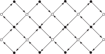
Let us consider a periodic spin lattice shown in Figure 1. We denote the set of vertices and edges of the lattice by $V$ and $E$. Note that the edges in the lattice are oriented: for an edge $e$ we denote its head (target) and tail (source) by $h(e),t(e)\in V$. Note also that around each vertex the orientations of the arrows alternate, and hence the number of incoming and outgoing arrows are the same. We color a vertex either black or white depending on the orientations of the arrows around the vertex. The lattice is then bipartite, i.e. an edge always connect two vertices of different colors. In this section we consider the square lattice, see however comments on generalization towards the end of section 3.

Figure 1: The spin lattice of the statistical mechanical model. The spins reside at the vertices of the lattice, and their nearest-neighbor interactions are represented by edges. The interaction is chiral, which is represented by the orientation of the edges. The color of a vertex (black or white) is determined by the orientations of arrows around it.

Spin Variables

We place spin variables at each lattice site $v\in V$: continuous $U(1)$ $N$-component spins $z_{v,1},\ldots,z_{v,N}\in e^{2\pi\sqrt{-1}\mathbb{R}}\,(|z_{v,i}|=1)$ and discrete $N$-component spins $m_{v,1},\ldots,m_{v,N}\in\mathbb{Z}_{r}$. We moreover impose the condition that

$$\prod_{i}z_{v,i}=1\ ,\qquad\sum_{i}m_{v,i}\equiv 0\quad(\textrm{mod }\,r)\ ,$$ (2.1)

and hence only $N-1$ of $z_{v,i}$ ($m_{v,i}$) are independent. In the following we collectively denote the spins at a vertex $v$ by $s_{v}=(z_{v},m_{v})$.

Note that we here consider classical (not quantum) statistical mechanical models, and spin here just refers to dynamical variables of the theory over which we sum/integrate over. On the boundary of the lattice we can impose periodic boundary conditions or fixed boundary conditions. In the latter case the boundary spins will be non-dynamical and the partition function will be a function of the values of the boundary spins. For simplicity we in the following will mostly consider periodic boundary conditions: the case with other boundary condition is similar, but some part of the analysis requires careful analysis of boundary effects.

Rapidity Parameters and Rapidity Lines

For the purpose of discussing integrability let us introduce extra parameters to the statistical model. These parameters $R_{e}$ are associated for edges $e\in E$, and we impose that condition that

$$\sum_{e:\textrm{ around a vertex }v}(1-R_{e})=2\ ,\quad\sum_{e:\textrm{ around a face }}R_{e}=2\ .$$ (2.2)

It is these parameters $R_{e}$ which enter into the definition of the partition function.

The conditions (2.2) do not have unique solutions. However the ambiguity can be naturally parametrized by the rapidity lines [18], which are drawn as red line in Figure 2. Rapidity lines contain the same data as the original spin lattice — we can recover the original lattice from the set of rapidity lines, following the rules in Figure 3.

Figure 2: The rapidity lines for the spin lattice of Figure 1, shown in red arrows.

Figure 3: We can reconstruct the spin lattice from the rapidity lines, following the rule shown here.

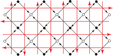
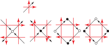
Let us denote the set of rapidity lines by $I$, and its element by $i\in I$. We associate a rapidity parameter (spectral parameter) $R_{i}$ to each rapidity line $i$. Given a solution $R_{e}$ to (2.2) we can modify $R_{e}$ to be

$$R_{e}^{\prime}:=R_{e}+R_{i}-R_{j}\ ,$$ (2.3)

when two rapidity lines $i,j$ pass through the edge $e$ as in Figure 4: We can then easily verify that $R_{e}^{\prime}$ also satisfy (2.2). Note that the overall shift of $R_{i}$ do not change the values of $R_{e}$, and hence is irrelevant for the statistical mechanical model of this paper.

Figure 4: The rapidity parameter for an edge $e$ is given by the difference of $R_{i}$ and $R_{j}$ associated with two rapidity lines $i,j$.

Boltzmann Weight

An edge $e\in E$, starting from a vertex $t(e)$ and ending on another $h(e)$, represents the nearest-neighbor interaction between the spins $s_{t(e)}$ and $s_{h(e)}$. The corresponding Boltzmann weight is given by

$$\begin{split}\mathbb{W}^{e}(R;s)&=\mathbb{W}^{e}_{R_{e}}(s_{t(e)},s_{h(e)})\\ &=\mathcal{W}^{e}_{0}(s_{t(e)},s_{h(e)})\,\prod_{1\leq i,j\leq N}\,\Gamma_{r,[\![m_{t(e),i}-m_{h(e),j}]\!]}\left((pq)^{\frac{R_{e}}{2}}\frac{z_{t(e),i}}{z_{h(e),j}};p,q\right)\ ,\end{split}$$ (2.4)

where $\Gamma_{r,[\![m]\!]}$ is the lens elliptic gamma function and $[\![m]\!]$ denotes $m$ modulo $r$ (see Appendix A). The multiplicative factor $\mathcal{W}^{e}_{0}(s_{t(e)},s_{h(e)})$ is given by

$$\begin{split}\mathcal{W}^{e}_{0}(s_{t(e)},s_{h(e)})=&\prod_{1\leq i,j\leq N}\Bigg{[}(p\,q)^{\frac{1}{4r}[\![m_{t(e),i}-m_{h(e),j}]\!][\![-m_{t(e),i}+m_{h(e),j}]\!](1-R_{e})}\\ &\times\,\left(\frac{p}{q}\right)^{-\frac{1}{12r}[\![m_{t(e),i}-m_{h(e),j}]\!][\![-m_{t(e),i}+m_{h(e),j}]\!](2[\![m_{t(e),i}-m_{h(e),j}]\!]-r)}\\ &\times\left(\frac{z_{t(e),i}}{z_{h(e),j}}\right)^{-\frac{1}{2r}[\![m_{t(e),i}-m_{h(e),j}]\!][\![-m_{t(e),i}+m_{h(e),j}]\!]}\Bigg{]}\ .\end{split}$$ (2.5)

Note that this Boltzmann weight is chiral (i.e. not reflection symmetric) $\mathbb{W}^{e}_{R_{e}}(s_{t(e)},s_{h(e)})\neq\mathbb{W}^{e}_{R_{e}}(s_{h(e)},s_{t(e)})$, except for the special case $N=2$.

We also include self-interactions among the different components of the spin $s_{v}$ at the same vertex $v$. The Boltzmann weight for the self-interaction at a vertex $v\in V$ is given by

$$\mathbb{S}^{v}(s)=\mathbb{S}^{v}(s_{v})=\left(\prod_{a=0}^{r-1}\frac{1}{n_{v,a}!}\right)\mathcal{S}^{v}_{0}(s_{v})\left(\Gamma_{r,0}(1;p,q)\right)^{-(N-1)}\prod_{i\neq j}\,\Gamma_{r,[\![m_{i}-m_{j}]\!]}\left(\frac{z_{v,i}}{z_{v,j}};p,q\right)^{-1}\ ,$$ (2.6)

where we denoted the number of $a\in\{0,1,\ldots,r-1\}$ in $\{m_{v,1},\ldots,m_{v,N}\}\in(\mathbb{Z}_{r})^{N}$ to be $n_{v,a}$: by definition we have $\sum_{a=0}^{k-1}n_{v,a}=N$. The multiplicative factor $\mathcal{S}^{v}_{0}(s_{v})$, which depends only on the discrete spins $m_{v}$ out of $s_{v}$, is given by

$$\mathcal{S}^{v}_{0}(s_{v})=(p\,q)^{-\frac{1}{4r}\sum_{i\neq j}[\![m_{v,i}-m_{v,j}]\!][\![-m_{v,i}+m_{v,j}]\!]}\ .$$ (2.7)

Note that the parameters $R_{e}$ do not appear in $\mathbb{S}^{v}$.

It is often possible to absorb this contribution into the definition of $\mathbb{W}^{e}(s_{t(e)},s_{h(e)})$, however it will be more natural to keep this factor for the identification with gauge theories.

Partition Function

The partition function is defined to be the statistical sum over all (continuous as well as discrete) spin configurations $\{s_{v}\}_{v\in V}$:

$$\begin{split}Z&=\sum_{s_{v}\,(v\in V)}\,\,\left(\prod_{v\in V}\mathbb{S}^{v}(s)\right)\left(\prod_{e\in E}\mathbb{W}^{e}(R;s)\right)\\ &=\sum_{m_{v}\,(v\in V)}\int_{|z_{v,m}|=1}\prod_{v\in V}\prod_{i=1}^{N-1}\frac{dz_{v,i}}{2\pi\sqrt{-1}z_{v,i}}\ \left(\prod_{v\in V}\mathbb{S}^{v}(z,m)\right)\left(\prod_{e\in E}\mathbb{W}^{e}(R;z,m)\right)\ ,\end{split}$$ (2.8)

where in the integrand we write $z_{v,N}$ in terms of $z_{v,i}$ $(i=1,\ldots,N-1)$ in terms of (2.1).

The total partition function (2.8) depends on two temperature-like parameters $p,q$ as well as rapidity parameters $R_{i}$. All of these parameters will appear inside the Boltzmann weight of the model. We can either regard $p,q$ as formal parameters, or impose $|p|,|q|<1$ for convergence of the Boltzmann weights.

Reformulation as IRF Model

The statistical mechanical model defined here can be reformulated either as a vertex model or an IRF (interaction-round-a-face) model [12]. To avoid repetition we in the following use the language of IRF models.

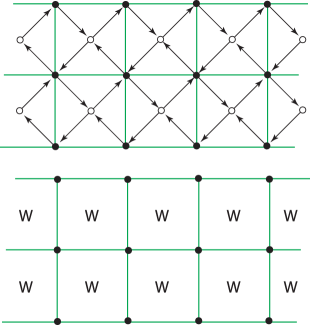
To define an IRF model, we simply integrate out spin variables at white vertices, while keeping those spins at black vertices. The remaining lattice is then a larger lattice colored green in Figure 5, and the Boltzmann weights are associated with the faces of the new lattice.

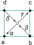
Suppose that we have a face $F$, with vertices $a,b,c,d$ as in Figure 6. We denote the rapidity parameters of four edges by $\alpha,\beta,\gamma,\delta$. It follows from (2.2) that they satisfy the relation $\alpha+\beta+\gamma+\delta=2$. We take the Boltzmann weight for the face $F$ to be

$$\begin{split}W(F)&=W\left(\begin{array}[]{cc}d&c\\ a&b\\ \end{array}\right)\\ &=\sqrt{\frac{\mathbb{W}_{2-\gamma-\delta}(d,c)\mathbb{W}_{2-\beta-\gamma}(b,c)}{\mathbb{W}_{2-\alpha-\beta}(a,b)\mathbb{W}_{2-\alpha-\delta}(a,d)}}\sqrt{\mathbb{S}^{a}\mathbb{S}^{c}}\,\sum_{g}\mathbb{S}^{g}\,\mathbb{W}_{\alpha}(a,g)\mathbb{W}_{\beta}(g,b)\mathbb{W}_{\gamma}(c,g)\mathbb{W}_{\delta}(g,d)\ ,\end{split}$$ (2.9)

where we used the short-handed notation $\mathbb{W}_{R_{e}}(t(e),h(e)):=\mathbb{W}^{e}_{R_{e}}(s_{t(e)},s_{h(e)})$.

The partition function (2.8) is can be re-written as the partition function of this IRF model:

$$Z=\sum_{F\textrm{: face}}W(F)\ .$$ (2.10)

Note that we have also included the Boltzmann weight for self-interactions $\mathbb{S}^{v}$ into the definition of the face weight (2.9). In (2.9) we have included a factor of

$$\sqrt{\frac{\mathbb{W}_{2-\gamma-\delta}(d,c)\mathbb{W}_{2-\beta-\gamma}(b,c)}{\mathbb{W}_{2-\alpha-\beta}(a,b)\mathbb{W}_{2-\alpha-\delta}(a,d)}}$$ (2.11)

for later convenience. This factor cancels out in the definition of the partition function (2.10), when we sum over faces of the IRF model. Note that we have $W_{R_{e}}(a,b)=W_{2-R_{e}}(b,a)^{-1}$ thanks to the relation (A.5).

Figure 5: The reformulation as an IRF model. The spins at white vertices are now integrated out, leaving only the black vertices defined on the green lattice. The Boltzmann weight $W$ is then associated with the faces of the new lattice. Alternative possibility is to exchange the role of white and black vertices, leading to another IRF model defined on the dotted lattice. The two IRF models nevertheless have the same partition function.

Figure 6: The face weight for the IRF model is determined from the Boltzmann weights for four edges, as well as those of four vertices, of the original spin lattice. We have denoted the four black vertices by $a,b,c,d$, and the weights for the edges connected by them by $\alpha,\beta,\gamma,\delta$. The first of the constraint equations (2.2) in this case means $\alpha+\beta+\gamma+\delta=2$.

2.2 Integrability

We now claim that the model discussed above is integrable. More precisely the model satisfies the star-star relation and consequently the YBE. This is the main result of the paper.

YBE

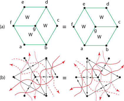
The integrability is defined by the famous Yang-Baxter equation. For the IRF model, the YBE is written as [19]

$$\begin{split}\sum_{g}W\left(\begin{array}[]{cc}f&g\\ a&b\\ \end{array}\right)W\left(\begin{array}[]{cc}e&d\\ f&g\\ \end{array}\right)W\left(\begin{array}[]{cc}d&c\\ g&b\\ \end{array}\right)=\sum_{g}W\left(\begin{array}[]{cc}e&g\\ f&a\\ \end{array}\right)W\left(\begin{array}[]{cc}g&c\\ a&b\\ \end{array}\right)W\left(\begin{array}[]{cc}e&d\\ g&c\\ \end{array}\right)\ ,\end{split}$$ (2.12)

which can be graphically represented as in Figure 7(a). The YBE implies the commutativity of the row-to-row transfer matrices, leading to an infinite number of conserved charges [19].

The YBE can also be written in terms of the original Boltzmann weights $\mathbb{S}^{v},\mathbb{W}^{e}$ (recall the relation (2.9)), which gives the relation in Figure 7(b). Most of the contributions from (2.11) cancel out, however some of them remain and appear in Figure 7(b) as extra arrows connecting two black vertices.

Figure 7: YBE for the IRF model (a) and for the rapidity lines (b).

Star-Star Relation

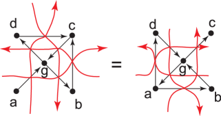
Instead of solving the YBE directly, we solve the the star-star (also called star-to-reversed-star) relation [15, 16]:

$$\begin{split}&\mathbb{W}_{2-\gamma-\delta}(d,c)\mathbb{W}_{2-\beta-\gamma}(b,c)\sum_{g}\mathbb{S}^{g}\,\mathbb{W}_{\alpha}(a,g)\mathbb{W}_{\beta}(g,b)\mathbb{W}_{\gamma}(c,g)\mathbb{W}_{\delta}(g,d)\\ &\quad=\mathbb{W}_{2-\alpha-\beta}(a,b)\mathbb{W}_{2-\alpha-\delta}(a,d)\sum_{g}\mathbb{S}^{g}\,\mathbb{W}_{\gamma}(g,a)\mathbb{W}_{\delta}(b,g)\mathbb{W}_{\alpha}(g,c)\mathbb{W}_{\beta}(d,g)\ .\end{split}$$ (2.14)

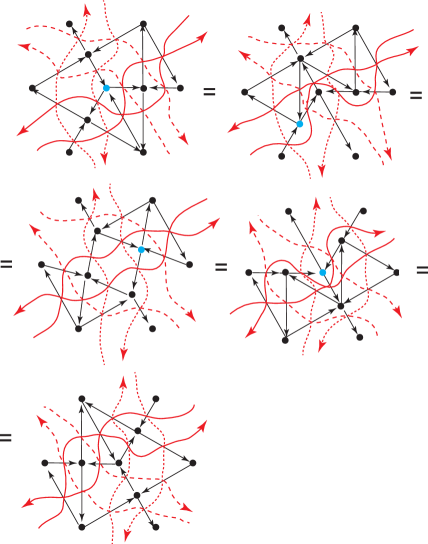
The graphical representations of this relation is given in Figure 8. We can directly verify that the YBE follows from the star-star relation, see Figure 9.

Figure 8: The graphical representation of the star-star relation.

Figure 9: YBE (Figure 7) follows from a sequence of star-star relations (Figure 8) [17]: in each step the star-star relation is taken around the blue vertex.

It would be desirable to mathematically prove the star-star relation. For the case with $r=1$ and general $N$, the star-star relation follows from the results of [20], as first pointed out by [21] (see also [22] for earlier work). In this paper the star-star relation will be derived from the considerations in supersymmetric gauge theory. This is be the topic of the next section.

3 Gauge Theory Origin

Let us now comment on the gauge-theoretic origin of our statistical mechanical model. Interestingly, each of the ingredients introduced in the previous section has a precise counterpart in 4d $\mathcal{N}=1$ supersymmetric gauge theories (see Table 1 in section 1). The gauge theory moreover gives generalization of the statistical mechanical model to spin lattices more general than the square lattices of the previous section. The discussion here will be brief since most of the ingredients here have been discussed in detail in [7, 8, 2].

3.1 Star-Star Relation as Seiberg Duality

The first step is to define a 4d $\mathcal{N}=1$ theory associated with the spin lattice.

The idea is to regard the spin lattice as the quiver diagram. Namely we associate an $SU(N)$ gauge group to a vertex $v\in V$, a bifundamental field to an edge $e\in E$, and a superpotential term (a trace of the product of bifundamentals) to a face of the spin lattice. Note that the orientation of the graph corresponds to the chirality of bifundamental multiplets.

It is believed in the literature that the resulting model flows in the IR to a non-trivial strongly-coupled fixed point. We assume in this paper that this is the case. Since the theory has many $U(1)$ global symmetries the $U(1)$ R-symmetry in the IR can be a mixture of UV $U(1)$ R-symmetry with other global $U(1)$ symmetries, leading to an ambiguity of the choice of the R-charge $R_{e}$ for a bifundamental at an edge $e\in E$. The ambiguities of the IR R-charges coming from the mixing with global symmetries can be parametrized as in (2.3) [27], where $R_{i}$ represents the global $U(1)$ symmetry associated with a rapidity line. The conditions (2.2) on the R-charges represent the vanishing of the beta-functions for the gauge couplings and superpotential couplings, respectively.

Now the crucial observation (which goes back to [14]) is that the star-star relation (2.14), when translated into the language of quiver gauge theories, is precisely the 4d $\mathcal{N}=1$ Seiberg duality [28]— in Figure 8 we have Seiberg duality for $N_{f}=2N$, where the global symmetry $SU(2N)$ is broken to $SU(N)\times SU(N)$ by a superpotential. The invariance of the partition function under star-star relation is then translated into the invariance of some quantity under 4d Seiberg duality.

There is one nice quantity which is indeed invariant under the Seiberg duality: the 4d lens index, the twisted partition function on $S^{1}\times S^{3}/\mathbb{Z}_{n}$. Here $S^{3}/\mathbb{Z}_{n}$ is the lens space, where $\mathbb{Z}_{n}$ acts on the Hopf fiber of $S^{3}$. Let us now discuss this quantity.

3.2 Partition Function from 4d Lens Index

The 4d lens index [1] is defined by

$$\mathcal{I}(p,q,u_{i})=\textrm{Tr}_{\,\mathcal{H}_{S^{3}/\mathbb{Z}_{r}}}\left[(-1)^{F}p^{\frac{E+j_{2}}{3}+j_{1}}q^{\frac{E+j_{2}}{3}-j_{1}}\right]\ ,$$ (3.1)

Here $\mathcal{H}_{S^{3}/\mathbb{Z}_{r}}$ is the Hilbert space on $\mathcal{H}_{S^{3}/\mathbb{Z}_{r}}$, $j_{1},j_{2}$ are the generators of $U(1)\times U(1)\in SU(2)\times SU(2)\sim SO(4)$ and $E$ the generator of translation along $S^{1}$. The fugacities for the global symmetries, which can be included in the definition of (3.1), is traded for the choice of R-charges. In other words the fugacity for the $i$-th global symmetry is given by $(pq)^{R_{i}}$.

The lens index is one of the most powerful quantities known in the literature for quantitative analysis of 4d $\mathcal{N}\geq 1$ supersymmetric gauge theories. It is more powerful than their $r=1$ counterparts (see [29, 30] for examples), and also reproduce many partition functions in lower dimensions, such as the 3d lens space partition function, the 3d superconformal index and the 2d sphere partition function ([31] and references therein).

Since the 4d lens index is an index, it is invariant under continuous deformations and is invariant under the RG flow, as long as we take into account the change of the R-charge under the RG flow (cf. [22]). This means that the index can be evaluated in the free field limit. The resulting expression coincides with expression found in section 2. For example, the spin variables $s_{v}=(z_{v},m_{v})$ are the Wilson lines for the $SU(N)$ gauge group at vertex $v\in V$. Since $\pi_{1}(S^{1}\times S^{3}/\mathbb{Z}_{r})=\mathbb{Z}\times\mathbb{Z}_{r}$, we have continuous Wilson lines $z_{v}=(z_{v,1},\ldots,z_{v,N})\in U(1)^{N}$, (with $\prod_{i}z_{v,i}=1$) along the $S^{1}$, or discrete Wilson lines $m_{v}=(m_{v,1},\ldots,m_{v,N})\in(\mathbb{Z}_{r})^{N}$ (with $\sum_{i}m_{v,i}=0$ modulo $r$) in the Hopf fiber direction of the manifold. This explains our choice of spin variables.

The Boltzmann weights $\mathbb{S}^{v},\mathbb{W}^{e}$ are the 1-loop determinants for vector and chiral multiplets (including the zero-point contributions $\mathcal{S}^{v}_{0},\mathcal{W}^{e}_{0}$), whose explicit expression can be found in [1, 31]. The chiral multiplet 1-loop determinant $\mathbb{W}^{e}$ corresponds to a nearest-neighbor interaction on the spin lattice since a bifundamental is charged only with respect to two $SU(N)$ gauge groups.

The star-star relation represents the Seiberg duality. The factors

$$\mathbb{W}_{2-\gamma-\delta}(d,c),\quad\mathbb{W}_{2-\beta-\gamma}(b,c),\quad\mathbb{W}_{2-\alpha-\beta}(a,b),\quad\mathbb{W}_{2-\alpha-\delta}(a,d)$$ (3.2)

in (2.14), which can be traced back to (2.11), represents the contributions from the mesons in the Seiberg duality. Since a meson $M$ couples to a quark $q$ and anti-quark $\tilde{q}$ by a superpotential term $W=\tilde{q}Mq$, and hence their R-charges should sum up to $2$. This is represented by the parametrizations of the rapidity parameters in (3.2) (in particular the numbers “2” there).

The statistical model of section 2.2 uses the square lattice (with periodic boundary conditions). However the gauge theory considerations apply to more general lattices determined from the rapidity lines, as long as the quiver defined from them is connected (more precisely this is the the admissibility conditions of [32, 7]). The vertex of the lattice can be of $2n$-valent ($n\geq 2$). The discussion of the star-star relation or equivalently the Seiberg duality works in exactly the same manner.

4 Further Comments

Several comments are now in order.

Specialization and Limits

Since the star-star relation is an equality, the limits and specializations of the model is still guaranteed to be integrable. We can for example take the fugacities $p,q$ to be at root of unity, or regard them as temperatures and take the high-temperature limit.

We can for example take $r=1$. The discrete spins $m_{v}$ are then frozen to be trivial values $m_{v}=0$, and the only non-trivial degrees of freedom are continuous $U(1)$ spins $z_{v,1},\ldots,z_{v,N}$. As discussed already in introduction, this coincides with the Bazhanov-Sergeev model [12] (up to the normalization constant of the partition function which is not essential for the discussion of integrability here). This model is known to reproduce a number of known integrable models [33, 11, 12], such as the Faddeev-Volkov model [34, 35], the chiral Potts model [36, 37] and the Kashiwara-Miwa model [38]. The last two models are different generalizations of the Fateev-Zamolodchikov model [39].

Interestingly, many of these models have discontinuous spins: the values of the continuous spins in the Bazhanov-Sergeev model are frozen to discrete values— this happens, for example, when we choose the temperature-like parameters $p,q$ to be at root of unity. It is interesting to ask whether the inverse procedure is possible, namely whether we can construct a model with all spins continuous such that our model is reproduced as a high-temperature limit. Such a model, if it exists, should be more powerful than the model discussed in this paper and could have some gauge theory implications, for example as an index of some 5d gauge theory.

Further Generalizations

There are several natural generalizations of our model. For example, we can take the rank of gauge groups (and hence the number of components of spins) to be $v$-dependent: the gauge group at $v$ is $SU(N_{v})$. It is straightforward to write down the corresponding statistical model. However, not all the possible values of $N_{v}$ are allowed since we have the ensure the absence of anomalies and the existence of the non-trivial IR fixed point. Moreover the ranks of the gauge groups will change under the Seiberg duality, and for this reason the corresponding YBE is more general than the one typically considered in integrable models. The same subtlety happens when we consider $S^{1}\times S^{2}$ index of 3d $\mathcal{N}=2$ quiver Chern-Simons-matter theories and the Giveon-Kutasov dualities [40] among them.

Comparison with Gauge/Bethe Correspondence

The Gauge/YBE correspondence (1.1) discussed in this paper is reminiscent of a similar correspondence in the literature, the Gauge/Bethe correspondence [41, 42]:

$$\mathcal{W}_{\rm eff}(\sigma)=Y(\sigma)\ .$$ (4.1)

On the left hand side of (4.1) we have the effective twisted super potential $\mathcal{W}_{\rm eff}(\sigma)$ of a 2d $\mathcal{N}=(2,2)$ theory as a function of the scalar in the twisted multiplet $\Sigma=\overline{D}_{+}D_{-}V$. On the right hand side we have the Yang-Yang function [43] $Y(\sigma)$. The derivative of this function gives the Bethe Ansatz equation, which coincides with the vacuum equation of the 2d $\mathcal{N}=(2,2)$ theory:

$$\exp\left(\frac{\partial\mathcal{W}_{\rm eff}}{\partial\sigma}\right)=\exp\left(\frac{\partial Y}{\partial\sigma}\right)=1\ .$$ (4.2)

While the two relations (1.1), (4.1) are similar, there are crucial differences between the two. One crucial difference is that in Gauge/YBE we have the partition function of an integrable model, whereas in Gauge/Bethe we have the Yang-Yang function. This is a huge difference when we want to find new integrable models from the correspondence.

In Gauge/Bethe correspondence it is in general rather hard to identify the corresponding integrable model for a given 2d $(2,2)$ theory—there is no general algorithm to recover the R-matrices from the Bethe Ansatz equation. In fact, it is not known in general whether such an integrable model really exists for a given 2d $\mathcal{N}=(2,2)$ theory.

This should be contrasted with the Gauge/YBE correspondence discussed in this paper. There the gauge theory answer directly gives precisely the R-matrix and the partition function of the integrable model, and the the reason why the model is integrable has a direct explanation from the 4d Seiberg duality. This direct relation was the reason that in this paper we could construct new integrable models from the correspondence.

Underlying Algebra

One of the systematic methods to construct solutions to YBE is to define the R-matrix as an intertwiner of the tensor product of representations. The relevant algebra for the $r=1$ case is the Sklyanin algebra [46] and their generalizations [47] (see e.g. [48]), which are 2-parameter deformations of the universal enveloping algebra $U(\mathfrak{gl}_{N})$. Such an algebra acts on the operators of a class of supersymmetric gauge theories, and plays the role similar to that of the Yangian in the Gauge/Bethe correspondence [41, 42].

Knot Invariants

It would be interesting to study the knots invariants associated with our solutions to the YBE (cf. [49]), see [50] for related discussion for the chiral Potts model.

5 Concluding Remarks

We proposed a 2d statistical spin lattice model with nearest-neighbor and self interactions. At each vertex we have a hybrid of continuous spins and discrete spins, each of which has $N$ components. The Boltzmann weights are given in (2.4), (2.6) and are written in terms of lens elliptic gamma functions (A.1). The model can be reformulated either as a vertex model or an IRF model.

The model is integrable (satisfy the star-star relation and hence the YBE) if we assume the invariance of the 4d lens index under the Seiberg duality. Alternatively, the mathematical proof of integrability can be thought of as another non-trivial test of the existence of non-trivial IR fixed points and the 4d Seiberg duality.

It is important to mathematically prove the integrability of the model. We can also study various properties of the model, such as free energies and correlation functions, and their gauge theory interpretations.

In this paper we have concentrated on the application of supersymmetric gauge theories to integrable models. We hope that our results are of interest to experts on integrable models. While this is interesting in its own right, experts on supersymmetric gauge theorists might be interested in a different question, namely if our results sheds any new light on our understanding of 4d $\mathcal{N}=1$ supersymmetric gauge theories.

In this respect, one fundamental question is whether the integrable structure discussed in this paper goes beyond the 4d lens index, and extends to the full physics of the IR fixed points.

We do not have the complete answer yet, however let us here point out that we have already identified dualities of quiver gauge theories corresponding to YBE: it is the sequence of four Seiberg dualities, and the quiver diagrams for the two theories are shown in Figure 7. This duality among supersymmetric gauge theories requires several $SU(N)$ gauge groups, which is probably the reason why it has not been paid much attention so far.

Recall that the R-matrix in integrable models is the linear map $R:V\otimes V\to V\otimes V$. This corresponds to a 4d $\mathcal{N}=1$ theory $\mathcal{T}[R]$, whose quiver diagram is a simply a “star” of Figure 6— if we un-gauge the gauge groups at the four black vertices, the theory is has global symmetry $SU(N)^{4}$, and the $SU(N)$ global symmetry plays the role similar to that of $V$. The counterpart of taking a product of R-matrices is to concatenate two quiver diagrams, by re-gauging the diagonal part of global $SU(N)\times SU(N)$ symmetries of the theories associated with the quivers. Finally, the counterpart of YBE is the following duality between two 4d $\mathcal{N}=1$ theories:

$$\mathcal{T}[R_{12}]\circ\mathcal{T}[R_{13}]\circ\mathcal{T}[R_{23}]\quad\textrm{is dual to}\quad\mathcal{T}[R_{23}]\circ\mathcal{T}[R_{13}]\circ\mathcal{T}[R_{12}]\ ,$$ (5.1)

where the symbol $\circ$ represents the gauging the diagonal subgroup of product global symmetries of two theories. The duality (5.1), which we call the Yang-Baxter duality, is more powerful than the equivalence of 4d lens indices. For example, the physical Hilbert spaces of the two theories should coincide in the IR, which can be thought of as a version of categorification of the Gauge/YBE correspondence.

The identification of the YBE with the duality (5.1) makes it clear that for the discussion of integrability we need to consider not a single theory, but a class of them related by gauging/un-gauging procedures: in the spirit of [53], what is relevant here is “integrability in theory space”.

It would be interesting to analyze the duality (5.1) further. The fact that the YBE is more general than the star-star relation in integrable model suggests that there should be generalizations of theory $\mathcal{T}[R]$ and dualities among them, which cannot be decomposed into Seiberg dualities. Such dualities will give an ultimate reason why gauge-theoretic quantities have integrable structures.

Appendix A Lens Elliptic Gamma Function

In this appendix we briefly summarize the definition and the properties of the lens elliptic gamma function used in the main text.

Let us choose a positive integer $r$ and an element $[\![m]\!]$ in $\mathbb{Z}_{r}$, where $[\![m]\!]$ represents the $m$ modulo $r$, i.e. $0\leq[\![m]\!]\leq r-1$ and $[\![m]\!]\equiv m$ modulo $r$. The lens elliptic gamma function elliptic gamma function $\Gamma_{r,[\![m]\!]}(x;p,q)$ is defined by

$$\Gamma_{r,[\![m]\!]}(x;p,q)=\frac{\displaystyle\prod_{n_{1},n_{2}\geq 0,\,n_{1}-n_{2}\equiv[\![-m]\!]\,(\textrm{mod }r)}\left(1-x^{-1}p^{n_{1}+1}q^{n_{2}+1}\right)}{\displaystyle\prod_{n_{1},n_{2}\geq 0,\,n_{1}-n_{2}\equiv[\![m]\!]\,(\textrm{mod }r)}\left(1-x\,p^{n_{1}}q^{n_{2}}\right)}\ .$$ (A.1)

We can rewrite this function as

$$\Gamma_{r,[\![m]\!]}(x;p,q)=\Gamma(xp^{[\![m]\!]};pq,p^{r})\,\Gamma(xq^{r-[\![m]\!]};pq,q^{r})\ ,$$ (A.2)

where $\Gamma(x;p,q)=\Gamma_{1,0}(x;p,q)$ is the ordinary elliptic gamma function found in the literature

$$\Gamma(x;p,q)=\prod_{n_{1},n_{2}\geq 0}\frac{1-x^{-1}p^{n_{1}+1}q^{n_{2}+1}}{1-x\,p^{n_{1}}q^{n_{2}}}\ .$$ (A.3)

For $m=0$ the lens elliptic gamma function simplifies to

$$\Gamma_{r,0}(x;p,q)=\Gamma(x;pq,p^{r})\,\Gamma(xq^{r};pq,q^{r})=\Gamma(x;p^{r},q^{r})\ .$$ (A.4)

We can easily prove the relations

$$\Gamma_{r,[\![-m]\!]}\left(\frac{pq}{x};p,q\right)=\Gamma_{r,[\![m]\!]}(x;p,q)^{-1}\ ,$$ (A.5)

References

- [1] F. Benini, T. Nishioka, and M. Yamazaki, 4d Index to 3d Index and 2d TQFT, Phys.Rev. D86 (2012) 065015, [arXiv:1109.0283].
- [2] D. Xie and M. Yamazaki, Network and Seiberg Duality, JHEP 1209 (2012) 036, [arXiv:1207.0811].
- [3] S. Franco, Bipartite Field Theories: from D-Brane Probes to Scattering Amplitudes, arXiv:1207.0807.
- [4] A. Hanany and A. Zaffaroni, On the realization of chiral four-dimensional gauge theories using branes, JHEP 9805 (1998) 001, [hep-th/9801134].
- [5] A. Hanany and A. M. Uranga, Brane boxes and branes on singularities, JHEP 9805 (1998) 013, [hep-th/9805139].
- [6] A. Hanany and K. D. Kennaway, Dimer models and toric diagrams, hep-th/0503149.
- [7] M. Yamazaki, Quivers, YBE and 3-manifolds, JHEP 1205 (2012) 147, [arXiv:1203.5784].
- [8] Y. Terashima and M. Yamazaki, Emergent 3-manifolds from 4d Superconformal Indices, Phys.Rev.Lett. 109 (2012) 091602, [arXiv:1203.5792].
- [9] J. Kinney, J. M. Maldacena, S. Minwalla, and S. Raju, An Index for 4 Dimensional Super Conformal Theories, Commun. Math. Phys. 275 (2007) 209–254, [hep-th/0510251].
- [10] C. Romelsberger, Counting chiral primaries in N = 1, d=4 superconformal field theories, Nucl.Phys. B747 (2006) 329–353, [hep-th/0510060].
- [11] V. V. Bazhanov and S. M. Sergeev, A Master solution of the quantum Yang-Baxter equation and classical discrete integrable equations, arXiv:1006.0651.
- [12] V. V. Bazhanov and S. M. Sergeev, Elliptic gamma-function and multi-spin solutions of the Yang-Baxter equation, Nucl.Phys. B856 (2012) 475–496, [arXiv:1106.5874].
- [13] V. V. Bazhanov, A. P. Kels, and S. M. Sergeev, Comment on star-star relations in statistical mechanics and elliptic gamma-function identities, arXiv:1301.5775.
- [14] V. Spiridonov, Elliptic beta integrals and solvable models of statistical mechanics, arXiv:1011.3798.
- [15] R. Baxter, The Yang-Baxter Equations and the Zamolodchikov Model, Physica D18 (1986) 321–347.
- [16] V. Bazhanov and R. Baxter, New solvable lattice models in three-dimensions, J.Statist.Phys. 69 (1992) 453–585.
- [17] R. Baxter, Star-triangle and star-star relations in statistical mechanics, Int.J.Mod.Phys. B11 (1997) 27–37.
- [18] R. Baxter, Solvable eight vertex model on an arbitrary planar lattice, Phil.Trans.Roy.Soc.Lond. 289 (1978) 315–346.
- [19] R. Baxter, Exactly solved models in statistical mechanics. Dover, 2007.
- [20] E. M. Rains, Transformations of elliptic hypergeometric integrals, Ann. of Math. (2) 171 (2010), no. 1 169–243.
- [21] F. Dolan and H. Osborn, Applications of the Superconformal Index for Protected Operators and q-Hypergeometric Identities to N=1 Dual Theories, Nucl.Phys. B818 (2009) 137–178, [arXiv:0801.4947].
- [22] C. Romelsberger, Calculating the Superconformal Index and Seiberg Duality, arXiv:0707.3702.
- [23] V. P. Spiridonov, On the elliptic beta function, Uspekhi Mat. Nauk 56 (2001), no. 1(337) 181–182.
- [24] K. D. Kennaway, Brane Tilings, Int.J.Mod.Phys. A22 (2007) 2977–3038, [arXiv:0706.1660].
- [25] M. Yamazaki, Brane Tilings and Their Applications, Fortsch.Phys. 56 (2008) 555–686, [arXiv:0803.4474]. Master’s Thesis.
- [26] J. J. Heckman, C. Vafa, D. Xie, and M. Yamazaki, String Theory Origin of Bipartite SCFTs, arXiv:1211.4587.
- [27] A. Hanany and D. Vegh, Quivers, tilings, branes and rhombi, JHEP 0710 (2007) 029, [hep-th/0511063].
- [28] N. Seiberg, Electric - magnetic duality in supersymmetric nonAbelian gauge theories, Nucl.Phys. B435 (1995) 129–146, [hep-th/9411149].
- [29] S. S. Razamat and M. Yamazaki, S-duality and the N=2 Lens Space Index, arXiv:1306.1543.
- [30] S. S. Razamat and B. Willett, Global properties of supersymmetric theories and the lens space, to appear.
- [31] M. Yamazaki, Four-dimensional superconformal index reloaded, Theor.Math.Phys. 174 (2013) 154–166.
- [32] K. Ueda and M. Yamazaki, A note on dimer models and McKay quivers, Commun.Math.Phys. 301 (2011) 723–747, [math/0605780].
- [33] V. V. Bazhanov, V. V. Mangazeev, and S. M. Sergeev, Faddeev-Volkov solution of the Yang-Baxter equation and discrete conformal symmetry, Nucl.Phys. B784 (2007) 234–258, [hep-th/0703041].
- [34] A. Volkov, Quantum Volterra model, Phys.Lett. A167 (1992) 345–355.
- [35] L. Faddeev and A. Y. Volkov, Abelian current algebra and the Virasoro algebra on the lattice, Phys. Lett. B 315 (1993), no. 3-4 311–318.
- [36] H. Au-Yang, B. M. McCoy, J. H. Perk, S. Tang, and M.-L. Yan, Commuting transfer matrices in the chiral Potts models: Solutions of Star triangle equations with genus 1, Phys.Lett. A123 (1987) 219–223.
- [37] R. Baxter, J. Perk, and H. Au-Yang, New solutions of the star triangle relations for the chiral Potts model, Phys.Lett. A128 (1988) 138–142.
- [38] M. Kashiwara and T. Miwa, A class of elliptic solutions to the star triangle relation, Nucl.Phys. B275 (1986) 121.
- [39] V. Fateev and A. Zamolodchikov, Selfdual solutions of the star triangle relations in Z(N) models, Phys.Lett. A92 (1982) 37–39.
- [40] A. Giveon and D. Kutasov, Seiberg Duality in Chern-Simons Theory, Nucl.Phys. B812 (2009) 1–11, [arXiv:0808.0360].
- [41] N. A. Nekrasov and S. L. Shatashvili, Supersymmetric vacua and Bethe ansatz, Nucl.Phys.Proc.Suppl. 192-193 (2009) 91–112, [arXiv:0901.4744].
- [42] N. A. Nekrasov and S. L. Shatashvili, Quantum integrability and supersymmetric vacua, Prog.Theor.Phys.Suppl. 177 (2009) 105–119, [arXiv:0901.4748].
- [43] C.-N. Yang and C. Yang, Thermodynamics of one-dimensional system of bosons with repulsive delta function interaction, J.Math.Phys. 10 (1969) 1115–1122.
- [44] N. A. Nekrasov, Seiberg-Witten Prepotential From Instanton Counting, Adv. Theor. Math. Phys. 7 (2004) 831–864, [hep-th/0206161].
- [45] N. A. Nekrasov and S. L. Shatashvili, Quantization of Integrable Systems and Four Dimensional Gauge Theories, arXiv:0908.4052.
- [46] E. Sklyanin, Some algebraic structures connected with the Yang-Baxter equation, Funct.Anal.Appl. 16 (1982) 263–270.
- [47] I. V. Cherednik, Some finite-dimensional representations of generalized Sklyanin algebras, Funktsional. Anal. i Prilozhen. 19 (1985), no. 1 89–90.
- [48] A. Zabrodin, Intertwining operators for Sklyanin algebra and elliptic hypergeometric series, J.Geom.Phys. 61 (2011) 1733–1754, [arXiv:1012.1228].
- [49] M. Wadati, T. Deguchi, and Y. Akutsu, Exactly Solvable Models and Knot Theory, Phys.Rept. 180 (1989) 247.
- [50] F. Y. Wu, P. Pant, and C. King, The chiral Potts model and its associated link invariant, J. Statist. Phys. 78 (1995), no. 5-6 1253–1276.
- [51] R. Kenyon, A. Okounkov, and S. Sheffield, Dimers and amoebae, Ann. of Math. (2) 163 (2006), no. 3 1019–1056.
- [52] H. Ooguri and M. Yamazaki, Emergent Calabi-Yau Geometry, Phys.Rev.Lett. 102 (2009) 161601, [arXiv:0902.3996].
- [53] M. Yamazaki, Entanglement in Theory Space, arXiv:1304.0762.