Finite-key analysis for measurement-device-independent quantum key distribution

Abstract

Quantum key distribution promises unconditionally secure communications. However, as practical devices tend to deviate from their specifications, the security of some practical systems is no longer valid. In particular, an adversary can exploit imperfect detectors to learn a large part of the secret key, even though the security proof claims otherwise. Recently, a practical approach—measurement-device-independent quantum key distribution—has been proposed to solve this problem. However, so far its security has only been fully proven under the assumption that the legitimate users of the system have unlimited resources. Here we fill this gap and provide a rigorous security proof against general attacks in the finite-key regime. This is obtained by applying large deviation theory, specifically the Chernoff bound, to perform parameter estimation. For the first time we demonstrate the feasibility of long-distance implementations of measurement-device-independent quantum key distribution within a reasonable time-frame of signal transmission.

I Introduction

It is unequivocal that quantum key distribution (QKD) QKDreview1 ; QKDreview2 needs to bridge the gap between theory and practice. In theory, QKD offers perfect security. In practice, however, it does not, as most practical devices behave differently from the theoretical models assumed in the security proofs. As a result, we face implementation loopholes, or so-called side-channels, which may be used by adversaries without being detected, as seen in recent attacks against certain commercial QKD systems sidechannelrefs2a ; sidechannelrefs1a ; sidechannelrefs2b ; sidechannelrefs2c ; sidechannelrefs1b ; sidechannelrefs1c ; sidechannelrefs2d ; sidechannelrefs2f ; sidechannelrefs2e .

There are two potential ways to guarantee security in the realisations of QKD. The first is to develop mathematical models that perfectly match the behaviour of physical apparatuses, and then incorporate this information into a new security proof. While this is plausible in theory, unfortunately it is very hard to realise in practice, if not impossible. The second alternative is to design new protocols and develop security proof techniques that are compatible with a wide class of device imperfections. This allows us to omit an accurate characterisation of real apparatuses. The most well-known example of such a solution is (full) device-independent QKD (diQKD) diqkdrefsa ; diqkdrefsb ; diqkdrefsc ; diqkdrefsd ; diqkdrefse . Here, the legitimate users of the system (typically called Alice and Bob) treat their devices as two quasi “black boxes”, i.e., they need to know which elements their boxes contain, but not how they fully function diqkdrefs2 . The security of diQKD relies on the violation of a Bell inequality bell1 ; bell2 , which certifies the presence of quantum correlations. Despite its beauty, however, this approach is highly impractical because it requires a loophole-free Bell test which at the moment is still unavailable Pearle1970 . Also, its secret key rate at practical distances is very limited Gisin2010a ; Gisin2010b .

Very recently, a novel approach has been introduced, which is fully practical and feasible to implement. This scheme is known as measurement-device-independent QKD (mdiQKD) mdiQKD and offers a clear avenue to bridge the gap between theory and practice. Its feasibility has been promptly demonstrated both in laboratories and via field-tests Rubenok2012a ; Rubenok2012b ; Rubenok2012c ; Rubenok2013a ; Zhiyuan:2013 . It successfully removes all (existing and yet to be discovered) detector side-channels sidechannelrefs2a ; sidechannelrefs2b ; sidechannelrefs2c ; sidechannelrefs2d ; sidechannelrefs2e ; sidechannelrefs2f , which, arguably, is the most critical part of most QKD implementations. Importantly, in contrast to diQKD this solution does not require that Alice and Bob perform a loophole-free Bell test; it is enough if they prove the presence of entanglement in a quantum state that is effectively distributed between them, just like in standard QKD schemes curty_prl2004 . In addition, now Alice and Bob may treat the measurement apparatus as a true “black box”, which may be fully controlled by the adversary. A slight drawback is that Alice and Bob need to characterise the quantum states [e.g., the polarisation degrees of freedom of phase-randomised weak coherent pulses (WCPs)] that they send through the channel. But, as this process can be verified in a protected environment outside the influence of the adversary, it is less likely to be a problem. For completeness, the readers can refer to charles2 where a characterisation of the prepared states is no longer required.

Nevertheless, so far the security of mdiQKD has only been proven in the asymptotic regime mdiQKD , which assumes that Alice and Bob have access to an unlimited amount of resources, or in the finite regime but only against particular types of attacks finitea ; finiteb . In summary, until now, a rigorous security proof of mdiQKD that takes full account of the finite size effects finite1 ; finite2 ; finite3 has appeared to be missing and, for this reason, the feasibility of long-distance implementations of mdiQKD within a reasonable time-frame of signal transmission has remained undemonstrated.

The main contributions of this work are twofold. First, in contrast to existing heuristic results on mdiQKD, we provide, for the first time, a security proof in the finite-key regime that is valid against general attacks, and satisfies the composability definition RennerThesis ; MullerQuadeRenner of QKD. Second, we apply large deviation theory, specifically a multiplicative form of the Chernoff bound cher , to perform the parameter estimation step. The latter is crucial to demonstrate that a long-distance implementation of mdiQKD (e.g., $150$ km of optical fiber with $0.2$ dB/km) is feasible within a reasonable time-frame. To obtain high secret key rates in this scenario, it is common to use decoy state techniques decoy1 ; decoy2 ; decoy3 , both for standard QKD protocols and mdiQKD. Here a key challenge is to estimate the transmittance and the quantum bit error rate (QBER) of the single-photon component of the signal at the presence of high losses (e.g., $30$ dB). We show that such an estimation problem can be solved using the Chernoff bound, as it provides good bounds for the parameters above even in the high-loss regime. We highlight that our results can be applied to other QKD protocols (e.g., the standard decoy state BB84 protocol decoy1 ; decoy2 ; decoy3 ) as well as to general experiments in quantum information.

II Security Definition

Prior to stating the protocol, let us quickly review the security framework RennerThesis ; MullerQuadeRenner that we are considering here. A general QKD protocol (executed by Alice and Bob) generates either a pair of bit strings $S_{\rm A}$ and $S_{\rm B}$, or a symbol $\perp$ to indicate the abort of the protocol. In general, the string of Alice, $S_{\rm A}$, can be quantum mechanically correlated with a quantum state that is held by the adversary. Mathematically, this situation is described by the classical-quantum state

$$\rho_{\rm AE}=\sum_{s}|s\rangle\langle s|\otimes\rho_{\rm E}^{s},$$

where $\{|s\rangle\}_{s}$ denotes an orthonormal basis for Alice’s system, and the subscript ${\rm E}$ indicates the system of the adversary.

Ideally, we say that a QKD protocol is secure if it satisfies two conditions, namely the correctness and the secrecy. The correctness condition is met if $S_{\rm A}=S_{\rm B}$, i.e., Alice’s and Bob’s bit strings are identical. The secrecy condition is met if $\rho_{\rm AE}=U_{\rm A}\otimes\rho_{\rm E}$, where $U_{\rm A}=\sum_{s}\frac{1}{|{\mathcal{S}}|}|s\rangle\langle s|$ is the uniform mixture of all possible values of the bit string $S_{\rm A}$. That is, the system of the adversary is completely decoupled from that of Alice.

Owing to the presence of errors, however, these two conditions can never be perfectly met. For example, in the finite-key regime it is impossible to guarantee $S_{\rm A}=S_{\rm B}$ with certainty. In practice, this implies that we need to allow for some minuscule errors. That is, we say that a QKD scheme is $\epsilon_{\textrm{cor}}$-correct if $\Pr[S_{\rm A}\not=S_{\rm B}]\leq\epsilon_{\textrm{cor}}$, i.e., the probability that Alice’s and Bob’s bit strings are not identical is not greater than $\epsilon_{\textrm{cor}}$. Similarly, we say that a protocol is $\epsilon_{\textrm{sec}}$-secret if

$$\frac{1}{2}\|\rho_{\rm AE}-U_{\rm A}\otimes\rho_{\rm E}\|_{1}\leq\epsilon_{\textrm{sec}},$$

where $\|\cdot\|_{1}$ denotes the trace norm. That is, the state $\rho_{\rm AE}$ is $\epsilon_{\textrm{sec}}$-close to the ideal situation described by $U_{\rm A}\otimes\rho_{\rm E}$. Thereby a QKD protocol is said to be $\epsilon$-secure if it is both $\epsilon_{\textrm{cor}}$-correct and $\epsilon_{\textrm{sec}}$-secret, with $\epsilon_{\textrm{cor}}+\epsilon_{\textrm{sec}}\leq\epsilon$.

With this security definition we are able to guarantee that the security of the protocol holds even when combined with other protocols, i.e., the protocol is secure in the so-called universally composable framework RennerThesis ; MullerQuadeRenner .

III Protocol definition

The setup is illustrated in Fig. 1. Alice and Bob use a laser source to generate quantum signals that are diagonal in the Fock basis. Instances of such sources include attenuated laser diodes emitting phase-randomised WCPs, triggered spontaneous parametric down-conversion sources, and practical single-photon sources. Each pulse is prepared in a different BB84 state bb84 , which is selected, for example, uniformly at random from two mutually unbiased bases, denoted as $\rm Z$ and $\rm X$. The signals are then sent to an untrusted relay Charles, who is supposed to perform a Bell state measurement that projects them into a Bell state. Also, Alice and Bob apply decoy state techniques decoy1 ; decoy2 ; decoy3 to estimate the gain (i.e., the probability that the relay outputs a successful result) and the QBER for various input photon-numbers.

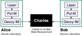
Figure 1: A schematic diagram of mdiQKD. Alice and Bob prepare quantum signals in different BB84 polarisation states bb84 with a polarisation modulator (Pol-M). Also, they use an intensity modulator (Decoy-IM) to generate decoy states. The signals are sent to an untrusted relay Charles, who is supposed to perform a Bell state measurement that projects the incoming signals into a Bell state. See the main text for details.

Next, Charles announces whether or not his measurements are successful, including the Bell states obtained. Alice and Bob keep the data that correspond to these instances and discard the rest. Also, they post-select the events where they employ the same basis. Finally, either Alice or Bob flips part of her/his bits to correctly correlate them with those of the other. See Table 1 for a detailed description of the different steps of the protocol.

1. State Preparation

Alice and Bob repeat the first four steps of the protocol for $i=1,\ldots,N$ till the conditions in the Sifting step are met. For each $i$, Alice chooses an intensity $a\in\{a_{\rm s},a_{\rm d_{1}},\ldots,a_{{\rm d}_{n}}\}$, a basis $\alpha\in\{{\rm Z,X}\}$, and a random bit $r\in\{0,1\}$ with probability $p_{a,\alpha}/2$. Here $a_{\rm s}$ ($a_{{\rm d}_{j}}$) is the intensity of the signal (decoy) states. Next, she generates a quantum signal (e.g., a phase-randomised WCP) of intensity $a$ prepared in the basis state of $\alpha$ given by $r$. Likewise, Bob does the same.

2. Distribution

Alice and Bob send their states to Charles via the quantum channel.

3. Measurement

If Charles is honest, he measures the signals received with a Bell state measurement. In any case, he informs Alice and Bob (via a public channel) of whether or not his measurement was successful. If successful, he reveals the Bell state obtained.

4. Sifting

If Charles reports a successful result, Alice and Bob broadcast (via an authenticated channel) their intensity and basis settings. For each Bell state $k$, we define two groups of sets: ${\mathcal{Z}}^{a,b}_{k}$ and ${\mathcal{X}}^{a,b}_{k}$. The first (second) one identifies signals where Charles declared the Bell state $k$ and Alice and Bob selected the intensities $a$ and $b$ and the basis $\rm Z$ ($\rm X$). The protocol repeats these steps until $|{\mathcal{Z}}^{a,b}_{k}|\geq N^{a,b}_{k}$ and $|{\mathcal{X}}^{a,b}_{k}|\geq M^{a,b}_{k}$ $\forall a,b,k$. Next, say Bob flips part of his bits to correctly correlate them with those of Alice (see Table 2). Afterwards, they execute the last steps of the protocol for each $k$.

5. Parameter Estimation

Alice and Bob use $n_{k}$ random bits from ${\mathcal{Z}}^{a_{\rm s},b_{\rm s}}_{k}$ to form the code bit strings $Z_{k}$ and $Z^{\prime}_{k}$, respectively. The remaining $R_{k}$ bits from ${\mathcal{Z}}^{a_{\rm s},b_{\rm s}}_{k}$ are used to compute the error rate $E^{a_{\rm s},b_{\rm s}}_{k}=\frac{1}{R_{k}}\sum_{l}r_{l}\oplus r^{\prime}_{l}$, where $r^{\prime}_{l}$ are Bob’s bits. If $E^{a_{\rm s},b_{\rm s}}_{k}>E_{\rm tol}$, Alice and Bob assign an empty string to $S_{k}$ and abort steps $6$ and $7$ for this $k$. The protocol only aborts if $E^{a_{\rm s},b_{\rm s}}_{k}>E_{\rm tol}$ $\forall k$. If $E^{a_{\rm s},b_{\rm s}}_{k}\leq{}E_{\rm tol}$, Alice and Bob use ${\mathcal{Z}}^{a,b}_{k}$ and ${\mathcal{X}}^{a,b}_{k}$ to estimate $n_{k,0}$, $n_{k,1}$ and $e_{k,1}$. The parameter $n_{k,0}$ ($n_{k,1}$) is a lower bound for the number of bits in $Z_{k}$ where Alice (Alice and Bob) sent a vacuum (single-photon) state. $e_{k,1}$ is an upper bound for the single-photon phase error rate. If $e_{k,1}>e_{{\rm tol}}$, an empty string is assigned to $S_{k}$ and steps $6$ and $7$ are aborted for this $k$, and the protocol only aborts if $e_{k,1}>e_{{\rm tol}}$ $\forall k$.

6. Error Correction

For those $k$ that passed the parameters estimation step, Bob obtains an estimate ${\hat{Z}}_{k}$ of $Z_{k}$ using an information reconciliation scheme. For this, Alice sends him ${\rm leak}_{{\rm EC},k}$ bits of error correction data. Next, Alice computes a hash of $Z_{k}$ of length $\lceil\log_{2}(4/\epsilon_{\rm cor})\rceil$ using a random universal₂ hash function, which she sends to Bob together with the hash RennerThesis . If ${\rm hash}({\hat{Z}}_{k})\neq{\rm hash}(Z_{k})$, Alice and Bob assign an empty string to $S_{k}$ and abort step $7$ for this $k$. The protocol only aborts if ${\rm hash}({\hat{Z}}_{k})\neq{\rm hash}(Z_{k})$ $\forall k$.

7. Privacy Amplification

If $k$ passed the error correction step, Alice and Bob apply a random universal₂ hash function to $Z_{k}$ and ${\hat{Z}}_{k}$ to extract two shorter strings of length $\ell_{k}$ RennerThesis . Alice obtains $S_{k}$ and Bob ${\hat{S}}_{k}$. The concatenation of $S_{k}$ (${\hat{S}}_{k}$) form the secret key $S_{\rm A}$ ($S_{\rm B}$).

Table 1: Protocol Definition.

	Bell state reported by Charles
Alice & Bob	$\quad|\psi^{-}\rangle$	$|\psi^{+}\rangle$	$|\phi^{-}\rangle$	$|\phi^{+}\rangle$
Z basis	Bit flip	Bit flip	-	-
X basis	Bit flip	-	Bit flip	-

Table 2: Post-processing of data in the sifting step. To guarantee that their bit strings are correctly correlated, say Bob applies a bit flip to part of his data, depending on the Bell state reported by Charles and the basis setting selected.

Since Charles’ measurement is basically used to post-select entanglement between Alice and Bob, the security of mdiQKD can be proven by using the idea of time reversal. Indeed, mdiQKD builds on the earlier proposals of time-reversed EPR protocols by Biham et al. biham and Inamori inamori , and combine them with the decoy state technique. The end result is the best of both worlds—high performance and high security. We note on passing that the idea of time reversal has also been previously used in other quantum information protocols including one-way quantum computation.

IV Security analysis

We now present one main result of our paper. It states that the protocol introduced above is both $\epsilon_{\textrm{cor}}$-correct and $\epsilon_{\textrm{sec}}$-secret, given that the length $\ell$ of the secret key $S_{\rm A}$ is selected appropriately for a given set of observed values. See Table 1 for the definition of the different parameters that we consider in this section.

The correctness of the protocol is guaranteed by its error correction step, where, for each possible Bell state $k$, Alice sends a hash of $Z_{k}$ to Bob, who compares it with the hash of ${\hat{Z}}_{k}$. If both hash values are equal, the protocol gives $S_{k}={\hat{S}}_{k}$ except with error probability $\epsilon_{\textrm{cor}}/4$. If ${\rm hash}({\hat{Z}}_{k})\neq{\rm hash}(Z_{k})$, it outputs the empty string (i.e., the protocol is trivially correct). Moreover, if the protocol aborts, the result is $\perp$, i.e., it is also correct. This guarantees that $S_{\rm A}=S_{\rm B}$ except with error probability less or equal than $\epsilon_{\textrm{cor}}$. Alternatively to this method, Alice and Bob may also guarantee the correctness of the protocol by exploiting properties of the error correcting code employed lut .

If the length $\ell_{k}$ of each bit string $S_{k}$, which forms the secret key $S_{\rm A}$, satisfies

$$\ell_{k}\leq n_{k,0}+n_{k,1}\left[1-h\left(e_{k,1}\right)\right]-{\rm leak}_{{\rm EC},k}-\log_{2}\frac{8}{\epsilon_{\rm cor}}-2\log_{2}\frac{2}{\varepsilon^{\prime}_{k}\hat{\varepsilon}_{k}}-2\log_{2}\frac{1}{2\varepsilon_{k,\textnormal{PA}}},$$ (1)

the protocol is $\epsilon_{\rm sec}$-secret, with $\epsilon_{\rm sec}=\sum_{k}\epsilon_{k,{\rm sec}}$ and $\epsilon_{k,{\rm sec}}=2(\varepsilon^{\prime}_{k}+2\varepsilon_{k,e}+\hat{\varepsilon}_{k})+\varepsilon_{k,\textnormal{b}}+\varepsilon_{k,0}+\varepsilon_{k,1}+\varepsilon_{k,\textnormal{PA}}$. In Eq. (1), $h(x)=-x\log_{2}{(x)}-(1-x)\log_{2}{(1-x)}$ is the binary Shannon entropy, and the parameters $\varepsilon_{k,0}$, $\varepsilon_{k,1}$, and $\varepsilon_{k,e}$ quantify, respectively, the probability that the estimation of the terms $n_{k,0}$, $n_{k,1}$ and $e_{k,1}$ is incorrect. A sketch of the proof of Eq. (1) can be found in Appendix A. There it is also explained the meaning of all the epsilons contained in the term $\epsilon_{k,{\rm sec}}$, which we omit here for simplicity. In the asymptotic limit of very large data blocks, the terms reducing the length of $S_{\rm A}$ due to statistical fluctuations may be neglected, and thus $\ell$ satisfies $\ell\leq\sum_{k}\max{\{n_{k,0}+n_{k,1}\left[1-h\left(e_{k,1}\right)\right]-{\rm leak}_{{\rm EC},k},0\}}$, as previously obtained in mdiQKD . That is, $n_{k,0}$ and $n_{k,1}$ provide a positive contribution to the secret key rate, while $n_{k,1}h\left(e_{k,1}\right)$ and ${\rm leak}_{{\rm EC},k}$ reduce it. The term $n_{k,1}h\left(e_{k,1}\right)$ corresponds to the information removed from $Z_{k}$ in the privacy amplification step of the protocol, while ${\rm leak}_{{\rm EC},k}$ is the information revealed by Alice in the error correction step.

The second main contribution of this work is an estimation method to obtain the relevant parameters $n_{k,0}$, $n_{k,1}$ and $e_{k,1}$ needed to evaluate the key rate formula above, when Alice and Bob send Charles a finite number $N$ of signals and use a finite number of decoy states. We solve this problem using techniques in large deviation theory. More specifically, we employ the Chernoff bound cher . It is important to note that standard techniques such as Azuma’s inequality azuma do not give very good bounds here. This is because this result does not consider the properties of the a priori distribution. Therefore, it is far from optimal for situations such as high loss or a highly bias coin flip, which are relevant in long-distance QKD. In contrast, the Chernoff bound takes advantage of the property of the distribution and provides good bounds even in a high-loss regime.

More precisely, we show that the estimation of $n_{k,0}$, $n_{k,1}$ and $e_{k,1}$ can be formulated as a linear program, which can be solved efficiently in polynomial time and gives the exact optimum even for large dimensions lpr . Importantly, this general method is valid for any finite number of decoy states used by Alice and Bob, and for any photon-number distribution of their signals. Also, for the typical scenario where Alice and Bob send phase-randomised WCPs together with two decoy states each, we solve analytically the linear program, and obtain analytical expressions for the parameters above, which can be used directly in an experiment. A sketch of the estimation method is given in Appendix B. For a detailed analysis of both estimation techniques we refer to the Appendices C and D.

V Discussion

In this section we analyse the behaviour of the secret key rate provided in Eq. (1). In our simulation, we consider that Alice and Bob encode their bits in the polarisation degrees of freedom of phase-randomised WCPs. Also, we assume that Charles uses the linear optics quantum relay illustrated in Fig. 2, which is able to identify two of the four Bell states. With this setup, a successful Bell state measurement corresponds to the observation of precisely two detectors (associated to orthogonal polarisations) being triggered. Note, however, that the results presented in this paper can be applied to other types of coding schemes like, for instance, phase or time-bin coding QKDreview1 ; QKDreview2 , and to any quantum operation that Charles may perform, as they solely depend on the measurement results that he announces.

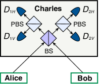
Figure 2: A schematic diagram of Charles’ measurement device. The signals from Alice and Bob interfere at a $50:50$ beam splitter (BS), which has on each end a polarising beam splitter (PBS) that projects the incoming photons into either horizontal ($H$) or vertical ($V$) polarisation states. A click in the single-photon detectors $D_{1H}$ and $D_{2V}$, or in $D_{1V}$ and $D_{2H}$, indicates a projection into the Bell state $|\psi^{-}\rangle=1/\sqrt{2}(|HV\rangle-|VH\rangle)$, while a click in $D_{1H}$ and $D_{1V}$, or in $D_{2H}$ and $D_{2V}$, implies a projection into the Bell state $|\psi^{+}\rangle=1/\sqrt{2}(|HV\rangle+|VH\rangle)$.

We use experimental parameters from param . But, whereas param considers a free-space channel, we assume a fiber-based channel with a loss of $0.2$ dB/km. The detection efficiency of the relay (i.e., the transmittance of its optical components together with the efficiency of its detectors) is $14.5\%$, and the background count rate is $6.02\times{}10^{-6}$. Moreover, we use a rather generic channel model that includes an intrinsic error rate which simulates the misalignment and instability of the optical system. This is done by placing a unitary rotation in both input arms of the $50:50$ beam splitter, and another unitary rotation in one of its output arms feihu . In addition, we fix the security bound to $\epsilon=10^{-10}$.

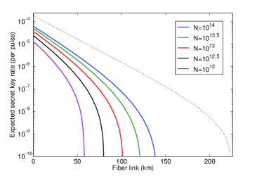
Figure 3: Expected key rate as function of the distance. Secret key rate $\ell/N$ in logarithmic scale for the protocol introduced in section III with phase-randomised WCPs as a function of the distance. The solid lines correspond to different values for the total number of signals $N$ sent by Alice and Bob. The overall misalignment in the channel is $1.5\%$, and the security bound $\epsilon=10^{-10}$. For simulation purposes we consider the following experimental parameters param : the loss coefficient of the channel is $0.2$ dB/km, the detection efficiency of the relay is $14.5\%$, and the background count rate is $6.02\times{}10^{-6}$. Our results show clearly that even with a realistic finite size of data, say $N=10^{12}$ to $10^{14}$, it is possible to achieve secure mdiQKD at long distances. In comparison, the dotted line represents a lower bound on the secret key rate for the asymptotic case where Alice and Bob send Charles infinite signals and use an infinite number of decoy settings.

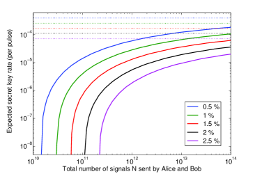
Figure 4: Expected key rate as function of the block size. The plot shows the secret key rate $\ell/N$ in logarithmic scale as a function of the total number of signals $N$ sent by Alice and Bob in the limit of zero distance. The security bound $\epsilon=10^{-10}$. The solid lines correspond to different values for the intrinsic error rate due to the misalignment and instability of the optical system. The horizontal dotted lines show the asymptotic rates. The experimental parameters are the ones described in the caption of Fig. 3. Our results show that, even for a finite size of signals sent by Alice and Bob, mdiQKD is robust to intrinsic errors due to basis misalignment and instability of the optical system.

The results are shown in Figs. 3-4 for the situation where Alice and Bob use two decoy states each. In this scenario, we obtain the parameters $n_{k,0}$, $n_{k,1}$ and $e_{k,1}$ using the analytical estimation procedure introduced above (see Appendix C for more details). The first figure illustrates the secret key rate (per pulse) $\ell/N$ as a function of the distance between Alice and Bob for different values of the total number of signals $N$ sent. We fix $\epsilon_{\rm cor}=10^{-15}$; this corresponds to a realistic hash tag size in practice RennerThesis . Also, we fix the intensity of the weakest decoy states to $a_{\rm d_{2}}=b_{\rm d_{2}}=5\times 10^{-4}$, since, in practice, is difficult to generate a vacuum state due to imperfect extinction. This value for $a_{\rm d_{2}}$ and $b_{\rm d_{2}}$ can be easily achieved with a standard intensity modulator. Moreover, for simplicity, we assume an error correction leakage that is a fixed fraction of the sifted key length $n_{k}$, i.e., ${\rm leak}_{{\rm EC},k}=n_{k}\zeta{}h(E_{k}^{a_{\rm s},b_{\rm s}})$, with $\zeta=1.16$ and where $h(\cdot)$ is again the binary Shannon entropy finite1 . In a realistic scenario, however, the value of $\zeta$ typically depends on the value of $n_{k}$, and when $n_{k}<10^{5}$ the parameter $\zeta$ may be bigger than $1.16$. For a given distance, we optimise numerically $\ell/N$ over all the free parameters of the protocol. This includes the intensities $a_{\rm s},a_{\rm d_{1}},b_{\rm s}$ and $b_{\rm d_{1}}$, the probability distributions $p_{a,\alpha}$ and $p_{b,\beta}$ in the state preparation step, the parameters $N_{k}^{a,b}$ and $M_{k}^{a,b}$ in the sifting step, the term $n_{k}$ in the parameter estimation step, and the different epsilons contained in $\epsilon_{\rm sec}$. Our simulation result shows clearly that mdiQKD is feasible with current technology and does not require high efficiency detectors for its implementation. If Alice and Bob use laser diodes operating at $1$ GHz repetition rate, and each of them sends $N=10^{13}$ signals, we find, for instance, that they can distribute a $1$ Mb secret key over a $75$ km fiber link in less than $3$ hours. This scenario corresponds to the red line shown in Fig. 3. Notice that, at telecom wavelengths, standard InGaAs detectors have modest detection efficiency of about $15\%$. Since mdiQKD requires two-fold coincidence rather than single-detection events, as is the case in the standard decoy state protocol, the key rate of mdiQKD is lower than that of the standard decoy state scheme. However, with high-efficiency detectors such as silicon detectors det1 in $800$nm or high-efficiency SSPDs det2 , the key rate of mdiQKD can be made comparable to that of the standard decoy state protocol.

The second figure illustrates $\ell/N$ as a function of $N$ for different values of the misalignment in the limit of zero distance. For comparison, this figure also includes the asymptotic secret key rate when Alice and Bob send an infinite number of signals and use an infinite number of decoy states mdiQKD . Our results show that significant secret key rates are already possible with $10^{11}$ signals, given that the error rate is not too large.

VI Conclusion

We have proved the security of mdiQKD in the finite-key regime against general attacks. This is the only known fully practical QKD protocol that offers an avenue to bridge the gap between theory and practice in QKD implementations. Importantly, our results clearly demonstrate that even with practical signals [e.g., phase-randomised weak coherent pulses (WCPs)] and a finite size of data (say $10^{12}$ to $10^{14}$ signals) it is possible to perform secure mdiQKD over long distances (up to about $150$ km).

To achieve high secret key rates in such high-loss regime, it is typical both for standard QKD schemes and mdiQKD to use decoy state techniques. A main challenge in this scenario is to obtain tight bounds for the gain and quantum bit error rate (QBER) of the single-photon components sent by Alice and Bob. We have shown that this estimation problem can be successfully solved using techniques in large deviation theory, more precisely, the Chernoff bound. This result takes advantage of the property of the distribution, and thus provides good bounds for the relevant parameters even in the presence of high losses, as is the case in QKD realisations.

Using the Chernoff bound we have rewritten the problem of estimating the gain and QBER of the single-photon signals as a linear program, which can be solved efficiently in polynomial time. This general method is valid for any finite number of decoy states, and for any photon-number distribution of the signals. It can be used, for instance, with laser diodes emitting phase-randomised WCPs, triggered spontaneous parametric down-conversion sources, and practical single-photon sources. Also, for the common scenario where Alice and Bob send phase-randomised WCPs together with two decoy states each, we have obtained tight analytical bounds for the quantities above. These results apply to different types of coding schemes like, for example, polarisation, phase or time-bin coding.

VII Acknowledgements

We thank Xiongfeng Ma and Johan Löfberg for valuable comments and stimulating discussions, and Lina M. Eriksson for comments on the writing and presentation of the paper. F. Xu. thanks the Paul Biringer Graduate Scholarship for financial support. We acknowledge support from the European Regional Development Fund (ERDF), the Galician Regional Government (projects CN2012/279 and CN 2012/260, “Consolidation of Research Units: AtlantTIC”), NSERC, the CRC program, the National Centre of Competence in Research QSIT, the Swiss NanoTera project QCRYPT, the FP7 Marie-Curie IAAP QCERT project, and CHIST-ERA project DIQIP. K.T. acknowledges support from the project “Secure photonic network technology” as part of “The project UQCC” by the National Institute of Information and Communications Technology (NICT) of Japan, and from the Japan Society for the Promotion of Science (JSPS) through its Funding Program for World-Leading Innovative R&D on Science and Technology (FIRST Program).

Appendix A Secrecy

Here, we briefly discuss on the secrecy of the protocol described in Table 1. To begin with, note that Alice and Bob obtain the error rate $E^{a_{\rm s},b_{\rm s}}_{k}$ using a random sample of ${\mathcal{Z}}_{k}^{a_{\rm s},b_{\rm s}}$ of size $R_{k}$. This means that when $E^{a_{\rm s},b_{\rm s}}_{k}$ satisfies the tolerated value $E_{\textnormal{tol}}$, the error rate between the strings $Z_{k}$ and $Z^{\prime}_{k}$, which we denote as $\xi^{a_{\rm s},b_{\rm s}}_{k}$, satisfies the following inequality written as conditional probability serf

$$\begin{aligned} \Pr\left[\xi^{a_{\rm s},b_{\rm s}}_{k}\geq E^{a_{\rm s},b_{\rm s}}_{k}+\chi(n_{k},R_{k},{\bar{\varepsilon}}_{k})|\Omega_{\textnormal{pass}}\right]\leq{\bar{\varepsilon}}_{k}^{2},\end{aligned}$$ (2)

where $\chi(x,y,z)=\sqrt{(y+x)(y+1)/(xy^{2})\ln{}z^{-1}}$. Here, the parameter $\Omega_{\textnormal{pass}}$ represents the event that all the tests performed during the realisation of the protocol satisfy the tolerated values.

Let $E^{\prime}_{k}$ denote the adversary’s information about $Z_{k}$ up to the error correction step in Table 1. By using a privacy amplification scheme based on two-universal hashing RennerThesis we can generate an $\epsilon_{k}$-secret string $S_{k}$ of length $\ell_{k}$, where $\varepsilon_{k}>0$, and

$$\begin{aligned} \epsilon_{k}\leq 8\varepsilon_{k}+2^{-\frac{1}{2}\left(H_{\min}^{4\varepsilon_{k}}\left(Z_{k}|E^{\prime}_{k}\right)-\ell_{k}\right)-1}.\end{aligned}$$ (3)

The function $H_{\min}^{4\varepsilon_{k}}\left(Z_{k}|E^{\prime}_{k}\right)$ denotes the smooth min-entropy RennerThesis ; minentr . It quantifies the average probability that the adversary guesses $Z_{k}$ correctly using the optimal strategy with access to $E^{\prime}_{k}$.

The term $E^{\prime}_{k}$ can be decomposed as $E^{\prime}_{k}=C_{k}E_{k}$, where $C_{k}$ is the information revealed by Alice and Bob during the error correction step, and $E_{k}$ is the adversary’s information prior to that step. Using a chain-rule for smooth entropies RennerThesis , we obtain

$$\begin{aligned} H_{\min}^{4\varepsilon_{k}}\left(Z_{k}|E^{\prime}_{k}\right)\geq H_{\min}^{4\varepsilon_{k}}\left(Z_{k}|E_{k}\right)-|C_{k}|,\end{aligned}$$ (4)

with $|C_{k}|\leq{\rm leak}_{{\rm EC},k}+\log_{2}(8/\epsilon_{\rm cor})$.

The bits of $Z_{k}$ can be distributed among three different strings: $Z_{k}^{0}$, $Z_{k}^{1}$ and $Z_{k}^{\rm rest}$. The first contains bits where Alice sent a vacuum state, the second where both Alice and Bob sent a single-photon state, and $Z_{k}^{\rm rest}$ includes the rest of bits. Using a result from Tomamichel , we have that

$$H_{\min}^{4\varepsilon_{k}}\left(Z_{k}|E_{k}\right)\geq H_{\min}^{\varepsilon^{\prime}_{k}+2\varepsilon^{\prime\prime}_{k}+(\hat{\varepsilon}_{k}+2\hat{\varepsilon}^{\prime}_{k}+\hat{\varepsilon}^{\prime\prime}_{k})}\left(Z_{k}^{0}Z_{k}^{1}Z_{k}^{\rm rest}|E_{k}\right)\geq n_{k,0}+H_{\min}^{\varepsilon^{\prime\prime}_{k}}\left(Z_{k}^{1}|Z_{k}^{0}Z_{k}^{\rm rest}E_{k}\right)-2\log_{2}\frac{2}{\varepsilon^{\prime}_{k}\hat{\varepsilon}_{k}},$$ (5)

where $4\varepsilon_{k}=\varepsilon^{\prime}_{k}+2\varepsilon^{\prime\prime}_{k}+(\hat{\varepsilon}_{k}+2\hat{\varepsilon}^{\prime}_{k}+\hat{\varepsilon}^{\prime\prime}_{k})$. Here, we have used the fact that $H_{\min}^{\hat{\varepsilon}^{\prime}_{k}}\left(Z_{k}^{\rm rest}|Z_{k}^{0}E_{k}\right)\geq 0$, and $H_{\min}^{\hat{\varepsilon}^{\prime\prime}_{k}}\left(Z_{k}^{0}|E_{k}\right)\geq H_{\min}^{0}\left(Z_{k}^{0}|E_{k}\right)=H_{\min}\left(Z_{k}^{0}\right)=n_{k,0}$. The latter arises because vacuum states contain no information about their bit values, which are uniformly distributed.

The next step is to obtain a lower bound for the term $H_{\min}^{\varepsilon^{\prime\prime}_{k}}\left(Z_{k}^{1}|Z_{k}^{0}Z_{k}^{\rm rest}E_{k}\right)$. Taking that Alice and Bob do the state preparation scheme perfectly in the $\rm Z$ and $\rm X$ bases (i.e., they prepare perfect BB84 states), we can re-write this quantity in terms of the smooth max-entropy between them, which is directly bounded by the strength of their correlations finite1 . More precisely, the entropic uncertainty relation gives us

$$H_{\min}^{\varepsilon^{\prime\prime}_{k}}\left(Z_{k}^{1}|Z_{k}^{0}Z_{k}^{\rm rest}E_{k}\right)\geq n_{k,1}-H_{\max}^{\varepsilon^{\prime\prime}_{k}}\left(X_{k}^{1}|X^{\prime}_{k}{}^{1}\right)\geq n_{k,1}-n_{k,1}h\left(e_{k,1}\right).$$ (6)

Combining Eqs. (3,4,5,6), we find that a secret key of length $\ell_{k}$ given by Eq. (1) gives an error of $\epsilon_{k}\leq 2(\varepsilon^{\prime}_{k}+2\varepsilon^{\prime\prime}_{k}+\hat{\varepsilon}_{k}+2\hat{\varepsilon}^{\prime}_{k}+\hat{\varepsilon}^{\prime\prime}_{k})+\varepsilon_{k,\textnormal{PA}}$. Finally, after composing the errors related with the estimation of $n_{k,0}$, $n_{k,1}$ and $e_{k,1}$, selecting $\hat{\varepsilon}^{\prime}_{k}$ and $\hat{\varepsilon}^{\prime\prime}_{k}$ equal to zero, and also removing the conditioning on $\Omega_{\textnormal{pass}}$, we obtain a security parameter $\epsilon_{k,{\rm sec}}$ given by

$$\epsilon_{k,{\rm sec}}=2(\varepsilon^{\prime}_{k}+2\varepsilon_{k,e}+\hat{\varepsilon}_{k})+\varepsilon_{k,\textnormal{b}}+\varepsilon_{k,0}+\varepsilon_{k,1}+\varepsilon_{k,\textnormal{PA}},$$ (7)

where $\varepsilon_{k,\textnormal{b}}={\bar{\varepsilon}}_{k}\sqrt{\Pr[\Omega_{\textnormal{pass}}]}$, and $\varepsilon_{k,0}$, $\varepsilon_{k,1}$ and $\varepsilon_{k,e}$ denote, respectively, the error probability in the estimation of $n_{k,0}$, $n_{k,1}$ and $e_{k,1}$.

Appendix B Sketch of the parameter estimation method

To simplify the discussion, let us consider the estimation of the parameter $n_{k,0}$. The method to obtain $n_{k,1}$ and $e_{k,1}$ follows similar arguments. The procedure can be divided into two steps. First, we calculate a lower bound for the number of indexes in ${\mathcal{Z}}^{a_{\rm s},b_{\rm s}}_{k}$ where Alice sent a vacuum state. This quantity is denoted as $m_{k,0}$. Second, we compute $n_{k,0}$ from $m_{k,0}$ using the Serfling inequality for random sampling without replacement serf .

In the first step we use a multiplicative form of the Chernoff bound cher for independent random variables, which does not require the prior knowledge on the population mean. More precisely, we use the following Claim.

Claim 1: Let $X_{1},X_{2},\ldots,X_{n}$, be a set of independent Bernoulli random variables that satisfy ${\rm Pr}(X_{i}=1)=p_{i}$, and let $X=\sum_{i=1}^{n}X_{i}$ and $\mu=E[X]=\sum_{i=1}^{n}p_{i}$, where $E[\cdot]$ denotes the mean value. Let $x$ be the observed outcome of $X$ for a given trial (i.e., $x\in{\mathbb{N}}^{+}$) and $\mu_{\rm L}=x-\sqrt{n/2\ln{(1/\epsilon)}}$ for certain $\epsilon>0$. When $(2\varepsilon^{-1})^{1/\mu_{\rm L}}\leq\exp{\left[3/(4\sqrt{2})\right]^{2}}$ and $({\hat{\varepsilon}}^{-1})^{1/\mu_{\rm L}}<\exp{(1/3)}$ for certain $\varepsilon,{\hat{\varepsilon}}>0$, we have that $x$ satisfies

$$x=\mu+\delta,$$ (8)

except with error probability $\gamma=\epsilon+\varepsilon+{\hat{\varepsilon}}$, where the parameter $\delta\in[-\Delta,{\hat{\Delta}}]$, with $\Delta=g(x,\varepsilon^{4}/16)$, ${\hat{\Delta}}=g(x,{\hat{\varepsilon}}^{3/2})$ and $g(x,y)=\sqrt{2x\ln{(y^{-1}})}$. Here $\varepsilon$ (${\hat{\varepsilon}}$) denotes the probability that $x<\mu-\Delta$ ($x>\mu+{\hat{\Delta}}$).

Importantly, the bounds ($-\Delta$ and ${\hat{\Delta}}$) on the fluctuation parameter $\delta$ that appears in Eq. (8) do not depend on the mean value $\mu$. A proof of Claim $1$ can be found in Appendix E. There, we introduce as well a generalised version of Claim $1$ for the cases where $(2\varepsilon^{-1})^{1/\mu_{\rm L}}>\exp{\left[3/(4\sqrt{2})\right]^{2}}$ and/or $({\hat{\varepsilon}}^{-1})^{1/\mu_{\rm L}}\geq\exp{(1/3)}$.

In order to apply this statement and be able to obtain the parameter $m_{k,0}$, we rephrase the protocol described in section III as follows. For each signal, we consider that Alice (Bob) first chooses a photon-number $n$ ($m$) and sends the signal to Charles, who declares whether his measurement is successful or not. After, Alice decides the intensity setting $a$, and Bob does the same. This virtual protocol is equivalent to the original one because the essence of decoy state QKD is precisely that Alice and Bob could have postponed the choice of which states are signals or decoys after Charles’ declaration of the successful events. This is possible because Alice’s and Bob’s observables commute with those of Charles. Note that for each specific combination of values $n$ and $m$, the observables that Alice and Bob use to determine whether a state is a signal or a decoy act on entirely different physical systems from those of Charles. This implies that Alice and Bob are free to postpone their measurement and thus their choice of signals and decoys. Also, this result shows that for each combination $n$ and $m$, the signal and decoy states provide a random sample of the population of all signals containing $n$ and $m$ photons respectively. Therefore, one can apply random sampling theory in classical statistics to the quantum problem.

Let ${\mathcal{S}}_{k,nm}$ denote the set that identifies those signals sent by Alice and Bob with $n$ and $m$ photons respectively, when they select the $\rm Z$ basis and Charles announces the Bell state $k$. And, let $|{\mathcal{S}}_{k,nm}|=S_{k,nm}$, and $p_{a,b|nm,{\rm Z}}$ be the conditional probability that Alice and Bob have selected the intensity settings $a$ and $b$, given that their signals contain, respectively, $n$ and $m$ photons prepared in the ${\rm Z}$ basis. Then, if we apply the above equivalence, independently of each other and for each signal Alice and Bob assign to each element in ${\mathcal{S}}_{k,nm}$ the intensity setting $a,b$, with probability $p_{a,b|nm,{\rm Z}}$.

Let $X_{i|k,nm}^{a,b}$ be $1$ if the $i$th element of ${\mathcal{S}}_{k,nm}$ is assigned to the intensity setting combination $a,b$, and otherwise $0$. And, let

$$X_{k}^{a,b}=\sum_{n,m}\sum_{i=1}^{S_{k,nm}}X_{i|k,nm}^{a,b},$$ (9)

with $\mu_{k}^{a,b}=E[X_{k}^{a,b}]=\sum_{n,m}p_{a,b|nm,{\rm Z}}S_{k,nm}$. Let $x_{k}^{a,b}=|{\mathcal{Z}}^{a,b}_{k}|$ denote the observed outcome of the random variable $X_{k}^{a,b}$ for a given trial. Then, if $(2\varepsilon_{a,b}^{-1})^{1/\mu_{k,{\rm L}}^{a,b}}\leq\exp{\left[3/(4\sqrt{2})\right]^{2}}$ and $({\hat{\varepsilon}}_{a,b}^{-1})^{1/\mu_{k,{\rm L}}^{a,b}}<\exp{(1/3)}$, with

$$\mu_{k,{\rm L}}^{a,b}=|{\mathcal{Z}}^{a,b}_{k}|-\sqrt{\sum_{a,b}|{\mathcal{Z}}_{k}^{a,b}|/2\ln{(1/\epsilon_{a,b})}},$$ (10)

the Claim above implies that

$$|{\mathcal{Z}}^{a,b}_{k}|=\sum_{n,m}p_{a,b|nm,{\rm Z}}S_{k,nm}+\delta_{a,b},$$ (11)

except with error probability $\gamma_{a,b}=\epsilon_{a,b}+\varepsilon_{a,b}+{\hat{\varepsilon}}_{a,b}$, where $\delta_{a,b}\in[-\Delta_{a,b},{\hat{\Delta}}_{a,b}]$, with $\Delta_{a,b}=g(|{\mathcal{Z}}^{a,b}_{k}|,\varepsilon_{a,b}^{4}/16)$ and ${\hat{\Delta}}_{a,b}=g(|{\mathcal{Z}}^{a,b}_{k}|,{\hat{\varepsilon}}_{a,b}^{3/2})$.

Using similar arguments, we find that the parameter $m_{k,0}$ can be written as

$$m_{k,0}={}\sum_{m}p_{a_{\rm s},b_{\rm s}|0m,{\rm Z}}S_{k,0m}-\Delta_{0},$$ (12)

except with error probability $\varepsilon_{0}$, where $\Delta_{0}=g(\sum_{m}p_{a_{\rm s},b_{\rm s}|0m,{\rm Z}}S_{k,0m},\varepsilon_{0})$.

Now, it is easy to find a lower bound for $m_{k,0}$. One only needs to minimise Eq. (12) given the linear constraints imposed by Eq. (11) for all $a,b$. This problem can be solved either using numerical tools as linear programming lpr or, for some particular cases, also analytical techniques. See the Appendices C and D for details.

The second step of the procedure is quite direct. Note that Alice forms her bit string $Z_{k}$ using $n_{k}$ random indexes from ${\mathcal{Z}}_{k}^{a_{\rm s},b_{\rm s}}$. Using serf we obtain

$$n_{k,0}=\max\bigg{\{}\bigg{\lfloor}{}n_{k}\frac{m_{k,0}}{|{\mathcal{Z}}^{a_{\rm s},b_{\rm s}}_{k}|}-n_{k}\Lambda(|{\mathcal{Z}}^{a_{\rm s},b_{\rm s}}_{k}|,n_{k},\varepsilon^{\prime\prime}_{k,0})\bigg{\rfloor},0\bigg{\}},$$ (13)

except with error probability

$$\varepsilon_{k,0}\leq\varepsilon^{\prime}_{k,0}+\varepsilon^{\prime\prime}_{k,0},$$ (14)

where $\varepsilon^{\prime}_{k,0}$ corresponds to the total error probability in the estimation of $m_{k,0}$, and the function $\Lambda(x,y,z)$ is defined as $\Lambda(x,y,z)=\sqrt{(x-y+1)\ln{(z^{-1})}/(2xy)}$.

Appendix C Analytical estimation of $n_{k,0}$, $n_{k,1}$ and $e_{k,1}$

This Appendix contains a general method to obtain an analytical expression for $n_{k,0}$, $n_{k,1}$ and $e_{k,1}$, when Alice and Bob use two decoy states each and the photon-number distribution of their signals is Poissonian.

That is, here we assume that $a\in{\mathcal{A}}=\{a_{\rm s},a_{{\rm d}_{1}},a_{{\rm d}_{2}}\}$, with $a_{\rm s}>a_{{\rm d}_{1}}>a_{{\rm d}_{2}}$, $b\in{\mathcal{B}}=\{b_{\rm s},b_{{\rm d}_{1}},b_{{\rm d}_{2}}\}$, with $b_{\rm s}>b_{{\rm d}_{1}}>b_{{\rm d}_{2}}$, and the probability that Alice (Bob) sends an $n$-photon ($m$-photon) signal when she (he) selects the intensity $a$ ($b$) is given by $p_{n|a}=e^{-a}a^{n}/n!$ ($p_{m|b}=e^{-b}b^{m}/m!$).

A similar estimation procedure has been recently introduced in Wang:2013 . Note, however, that Wang:2013 considers one of the two decoy signals a vacuum state, which is very hard to guarantee in practical QKD implementations, due to the finite extinction ratio of the intensity modulator decoy:2009 . Also, Wang:2013 analyses the asymptotic regime where Alice and Bob send an arbitrarily large number of signals. Below we introduce a general analytical method that overcomes both difficulties.

We begin by introducing some notations. Let $S_{k,nm}$ denote the number of signals sent by Alice and Bob with $n$ and $m$ photons respectively, when they select the basis ${\rm Z}$ and Charles declares the Bell state $k$. As noted in Appendix B, for each combination of values $n$ and $m$, the signal and decoy states provide a random sample of the population of all signals containing $n$ and $m$ photons respectively. Therefore, standard large deviation theory techniques such as the Chernoff bound apply [34]. In particular, when both

$$\left(2\varepsilon_{a,b}^{-1}\right)^{1/\mu_{k,{\rm L}}^{a,b}} \leq e^{\left[3/(4\sqrt{2})\right]^{2}},$$

$$\left({\hat{\varepsilon}}_{a,b}^{-1}\right)^{1/\mu_{k,{\rm L}}^{a,b}} < e^{1/3},$$ (15)

with the parameter $\mu_{k,{\rm L}}^{a,b}$ given by

$$\mu_{k,{\rm L}}^{a,b}=|{\mathcal{Z}}^{a,b}_{k}|-\sqrt{\sum_{a,b}|{\mathcal{Z}}_{k}^{a,b}|/2\ln{(1/\epsilon_{a,b})}},$$ (16)

we have that $|{\mathcal{Z}}^{a,b}_{k}|$ can be written as

$$|{\mathcal{Z}}^{a,b}_{k}|=\sum_{n,m}p_{a,b|nm,{\rm Z}}S_{k,nm}+\delta_{a,b},$$ (17)

except with error probability $\gamma_{a,b}=\epsilon_{a,b}+\varepsilon_{a,b}+{\hat{\varepsilon}}_{a,b}$, where $\varepsilon_{a,b}$ refers to the failure probability of one side, whereas ${\hat{\varepsilon}}_{a,b}$ refers to that of the other side. The total failure probability is thus the sum and is denoted by $\gamma_{a,b}$. The parameter $\delta_{a,b}\in[-\Delta_{a,b},{\hat{\Delta}}_{a,b}]$, with $\Delta_{a,b}=g(|{\mathcal{Z}}^{a,b}_{k}|,\varepsilon_{a,b}^{4}/16)$ and ${\hat{\Delta}}_{a,b}=g(|{\mathcal{Z}}^{a,b}_{k}|,{\hat{\varepsilon}}_{a,b}^{3/2})$, and the function $g(x,y)=\sqrt{2x\ln{(y^{-1}})}$. A proof of Eq. (17) can be found in Appendix B (see also Appendix E), where we introduce as well a generalised version of it for the cases where Eq. (C) is not satisfied.

C.1 Estimation of $n_{k,0}$

The procedure to obtain $n_{k,0}$ can be decomposed into two steps. First, we calculate a lower bound for the number of indexes in ${\mathcal{Z}}^{a_{\rm s},b_{\rm s}}_{k}$ where Alice sent a vacuum state. This quantity is denoted as $m_{k,0}$, and can be written as

$$m_{k,0}={}\sum_{m}p_{a_{\rm s},b_{\rm s}|0m,{\rm Z}}S_{k,0m}-\Delta_{0},$$ (18)

except with error probability $\varepsilon_{0}$, where $\Delta_{0}=g(\sum_{m}p_{a_{\rm s},b_{\rm s}|0m,{\rm Z}}S_{k,0m},\varepsilon_{0})$. The proof of Eq. (18) follows similar lines as the proof of Eq. (17) [34]. Second, we use the Serfling inequality for random sampling without replacement [49] to compute $n_{k,0}$ from $m_{k,0}$.

Let us begin with the first step. According to Eq. (18), to compute $m_{k,0}$ we need to search for a lower bound for

$$\sum_{m}p_{a_{\rm s},b_{\rm s}|0m,{\rm Z}}S_{k,0m}.$$ (19)

The probability $p_{a,b|nm,{\rm Z}}$ can be written as

$$p_{a,b|nm,{\rm Z}}=\frac{p_{n|a}p_{m|b}p_{a,b,{\rm Z}}}{\sum_{a,b}p_{n|a}p_{m|b}p_{a,b,{\rm Z}}},$$ (20)

where $p_{a,b,{\rm Z}}$ denotes the probability that Alice and Bob send signals in the $\rm Z$ basis with intensity $a$ and $b$ respectively. Using the fact that $p_{n|a}=e^{-a}a^{n}/n!$ and $p_{m|b}=e^{-b}b^{m}/m!$ we obtain

$$p_{a,b|nm,{\rm Z}}=\frac{1}{n!m!\tau_{nm}}e^{-(a+b)}a^{n}b^{m}p_{a,b,{\rm Z}},$$ (21)

with the term $\tau_{nm}$ given by

$$\tau_{nm}=\frac{1}{n!m!}\sum_{a,b}e^{-(a+b)}a^{n}b^{m}p_{a,b,{\rm Z}}.$$ (22)

Hence, we have that Eq. (19) can be expressed as

$$p_{a_{\rm s},b_{\rm s},{\rm Z}}e^{-(a_{\rm s}+b_{\rm s})}T_{k,0m},$$ (23)

with the parameter $T_{k,0m}$ given by

$$T_{k,0m}=\sum_{m}\frac{b_{\rm s}^{m}}{m!}{\tilde{S}}_{k,0m},$$ (24)

where ${\tilde{S}}_{k,nm}=S_{k,nm}/\tau_{nm}$. In so doing, we reduce the problem of finding $m_{k,0}$ to that of calculating a lower bound for $T_{k,0m}$. This is what we do next.

Our starting point is Eq. (17), which now can be rewritten as

$$|{\tilde{\mathcal{Z}}}^{a,b}_{k}|=\sum_{n,m}\frac{a^{n}b^{m}}{n!m!}{\tilde{S}}_{k,nm}+{\tilde{\delta}}_{a,b},$$ (25)

with $|{\tilde{\mathcal{Z}}}^{a,b}_{k}|=e^{a+b}|{\mathcal{Z}}^{a,b}_{k}|/p_{a,b,{\rm Z}}$ and ${\tilde{\delta}}_{a,b}=e^{a+b}\delta_{a,b}/p_{a,b,{\rm Z}}$. Next, we combine the quantities given by Eq. (25) in such a way that we can cancel out the terms of the form ${\tilde{S}}_{k,1m}$. For this, we define the parameter $L_{k,a_{0},a_{1}}$ as

$$L_{k,a_{0},a_{1}}=a_{0}|{\tilde{\mathcal{Z}}}^{a_{1},b_{\rm s}}_{k}|-a_{1}|{\tilde{\mathcal{Z}}}^{a_{0},b_{\rm s}}_{k}|=(a_{0}-a_{1})T_{k,0m}+\sum_{\begin{subarray}{c}m=0\\ n\geq 2\end{subarray}}\frac{a_{0}a_{1}^{n}-a_{1}a_{0}^{n}}{n!m!}b_{\rm s}^{m}{\tilde{S}}_{k,nm}+a_{0}{\tilde{\delta}}_{a_{1},b_{\rm s}}-a_{1}{\tilde{\delta}}_{a_{0},b_{\rm s}},$$ (26)

with $a_{0},a_{1}\in{\mathcal{A}}$. Note that when $a_{0}>a_{1}$ the second term on the r.h.s. of Eq. (26) is always less or equal to zero. This means, in particular, that $L_{k,a_{0},a_{1}}\leq(a_{0}-a_{1})T_{k,0m}+a_{0}{\hat{\Gamma}}_{a_{1},b_{\rm s}}+a_{1}{\Gamma}_{a_{0},b_{\rm s}}$. Here, for the fluctuation terms ${\tilde{\delta}}_{a,b}$, we have used the fact that they lay in the interval $[-\Gamma_{a,b},{\hat{\Gamma}}_{a,b}]$, with $\Gamma_{a,b}=e^{a+b}\Delta_{a,b}/p_{a,b,{\rm Z}}$ and ${\hat{\Gamma}}_{a,b}=e^{a+b}{\hat{\Delta}}_{a,b}/p_{a,b,{\rm Z}}$, except with error probability $\gamma_{a,b}$.

As a result we find, therefore, that

$$T_{k,0m}\geq\max_{\begin{subarray}{c}a_{0},a_{1}\in{\mathcal{A}}\\ a_{0}>a_{1}\end{subarray}}\left\{\frac{L_{k,a_{0},a_{1}}-a_{0}{\hat{\Gamma}}_{a_{1},b_{\rm s}}-a_{1}{\Gamma}_{a_{0},b_{\rm s}}}{a_{0}-a_{1}},0\right\},$$ (27)

except with error probability $\sum_{a}\gamma_{a,b_{\rm s}}$.

Moving to the second step, we use the Serfling inequality [49] to compute $n_{k,0}$ from $m_{k,0}$. This is so because Alice forms her bit string $Z_{k}$ using $n_{k}$ random indexes from ${\mathcal{Z}}_{k}^{a_{\rm s},b_{\rm s}}$. We obtain

$$n_{k,0}=\max\left\{\bigg{\lfloor}{}n_{k}\frac{m_{k,0}}{|{\mathcal{Z}}^{a_{\rm s},b_{\rm s}}_{k}|}-n_{k}\Lambda(|{\mathcal{Z}}^{a_{\rm s},b_{\rm s}}_{k}|,n_{k},\varepsilon^{\prime\prime}_{k,0})\bigg{\rfloor},0\right\},$$ (28)

except with error probability

$$\varepsilon_{k,0}\leq\varepsilon^{\prime}_{k,0}+\varepsilon^{\prime\prime}_{k,0},$$ (29)

where the function $\Lambda(x,y,z)$ is defined as $\Lambda(x,y,z)=\sqrt{(x-y+1)\ln{(z^{-1})}/(2xy)}$, and $\varepsilon^{\prime}_{k,0}\leq\varepsilon_{0}+\sum_{a}\gamma_{a,b_{\rm s}}$.

C.2 Estimation of $n_{k,1}$

To estimate $n_{k,1}$ we employ the same two-step method that we used to obtain $n_{k,0}$. That is, we first compute a lower bound for the number of indexes in ${\mathcal{Z}}^{a_{\rm s},b_{\rm s}}_{k}$ where both Alice and Bob sent a single-photon. We shall denote this quantity as $m_{k,1}$, which can be written as

$$m_{k,1}={}p_{a_{\rm s},b_{\rm s}|11,{\rm Z}}S_{k,11}-\Delta_{1},$$ (30)

except with error probability $\varepsilon_{1}$, where the parameter $\Delta_{1}=g(p_{a_{\rm s},b_{\rm s}|11,{\rm Z}}S_{k,11},\varepsilon_{1})$. Again, this statement can be proven with similar arguments to those used to prove Eq. (17). Second, we calculate $n_{k,1}$ from $m_{k,1}$ using the Serfling inequality [49].

According to Eq. (30), to compute $m_{k,1}$ we need to search for a lower bound for $S_{k,11}$. This is what we do next. Our starting point is Eq. (25). The estimation method is then divided into two steps. First, we cancel the terms ${\tilde{S}}_{k,0m}$ and ${\tilde{S}}_{k,n0}$ using Gaussian elimination. Second, we cancel either the parameter ${\tilde{S}}_{k,12}$ or ${\tilde{S}}_{k,21}$, depending on the combination of intensities that are used in the first step; this will become clear below.

Let us begin with the first step. For this, we introduce a vector of intensities $v=[a_{0},a_{1},b_{0},b_{1}]$ that satisfies $a_{0}>a_{1}$ and $b_{0}>b_{1}$, with $a_{i}\in{\mathcal{A}}$ and $b_{i}\in{\mathcal{B}}$. Then, we find that the parameters $G_{k,v}$ defined below do not contain any term of the form ${\tilde{S}}_{k,0m}$ or ${\tilde{S}}_{k,n0}$, with

$$G_{k,v}=|{\tilde{\mathcal{Z}}}^{a_{0},b_{0}}_{k}|+|{\tilde{\mathcal{Z}}}^{a_{1},b_{1}}_{k}|-|{\tilde{\mathcal{Z}}}^{a_{0},b_{1}}_{k}|-|{\tilde{\mathcal{Z}}}^{a_{1},b_{0}}_{k}|.\quad\quad$$ (31)

Next, we move to the second step. Here, we select another vector $v^{\prime}=[a^{\prime}_{0},a^{\prime}_{1},b^{\prime}_{0},b^{\prime}_{1}]$ that fulfils the same conditions as $v$, and, moreover, satisfies the following constraints: $a_{i}=a^{\prime}_{j}$, $a_{i\oplus 1}>a^{\prime}_{j\oplus 1}$, $b_{i^{\prime}}=b^{\prime}_{j^{\prime}}$ and $b_{i^{\prime}\oplus 1}>b^{\prime}_{j^{\prime}\oplus 1}$ for certain $i,j,i^{\prime},j^{\prime}=0,1$, and where the symbol $\oplus$ denotes the modulo-$2$ addition. Then, we need to consider two cases.

Case $1$: If $(a_{0}+a_{1})/(a^{\prime}_{0}+a^{\prime}_{1})>(b_{0}+b_{1})/(b^{\prime}_{0}+b^{\prime}_{1})$, we define the parameter $J_{k,v,v^{\prime}}$ as

$$J_{k,v,v^{\prime}}=(b_{0}^{2}-b_{1}^{2})(a_{0}-a_{1})G_{k,v^{\prime}}-(b_{0}^{\prime 2}-b_{1}^{\prime 2})(a^{\prime}_{0}-a^{\prime}_{1})G_{k,v}.$$ (32)

Using Eqs. (25)-(31), we can rewrite $J_{k,v,v^{\prime}}$ as

$$J_{k,v,v^{\prime}} = \sum_{n,m=1}^{\infty}\frac{c_{nm}}{n!m!}{\tilde{S}}_{k,nm}+\delta_{k,v,v^{\prime}},$$ (33)

where the coefficients $c_{nm}$ and $\delta_{k,v,v^{\prime}}$ are given by

$$c_{nm} = (b_{0}^{2}-b_{1}^{2})(a_{0}-a_{1})(a_{0}^{\prime n}-a_{1}^{\prime n})(b_{0}^{\prime m}-b_{1}^{\prime m})-(b_{0}^{\prime 2}-b_{1}^{\prime 2})(a^{\prime}_{0}-a^{\prime}_{1})(a_{0}^{n}-a_{1}^{n})(b_{0}^{m}-b_{1}^{m}),$$ (34)

$$\delta_{k,v,v^{\prime}} = (b_{0}^{2}-b_{1}^{2})(a_{0}-a_{1})\delta_{k,v^{\prime}}-(b_{0}^{\prime 2}-b_{1}^{\prime 2})(a^{\prime}_{0}-a^{\prime}_{1})\delta_{k,v},$$

and the parameters $\delta_{k}^{v}$ and $\delta_{k}^{v^{\prime}}$ have the form

$$\delta_{k}^{v} = {\tilde{\delta}}_{a_{0},b_{0}}+{\tilde{\delta}}_{a_{1},b_{1}}-{\tilde{\delta}}_{a_{0},b_{1}}-{\tilde{\delta}}_{a_{1},b_{0}},$$

$$\delta_{k}^{v^{\prime}} = {\tilde{\delta}}_{a^{\prime}_{0},b^{\prime}_{0}}+{\tilde{\delta}}_{a^{\prime}_{1},b^{\prime}_{1}}-{\tilde{\delta}}_{a^{\prime}_{0},b^{\prime}_{1}}-{\tilde{\delta}}_{a^{\prime}_{1},b^{\prime}_{0}}.$$ (35)

From the conditions above, it is easy to show that $c_{11}\geq{}0$ and $c_{nm}\leq{}0$ when $n+m\geq 3$. For simplicity, however, we de not include such proofs here. Combining these results with Eq. (33), we obtain

$${\tilde{S}}_{k,11}\geq\frac{1}{c_{11}}\left(J_{k,v,v^{\prime}}-\delta_{k,v,v^{\prime}}\right).$$ (36)

Now, we need to compute an upper bound for $\delta_{k,v,v^{\prime}}$. Using the fact that ${\tilde{\delta}}_{a,b}\in[-\Gamma_{a,b},{\hat{\Gamma}}_{a,b}]$ except with error probability $\gamma_{a,b}$, we obtain that $\delta_{k,v,v^{\prime}}\leq\Gamma_{k,v,v^{\prime}}$ with

$$\Gamma_{k,v,v^{\prime}} = (b_{0}^{2}-b_{1}^{2})(a_{0}-a_{1})({\hat{\Gamma}}_{a^{\prime}_{0},b^{\prime}_{0}}+{\hat{\Gamma}}_{a^{\prime}_{1},b^{\prime}_{1}}+{\hat{\Gamma}}_{a^{\prime}_{0},b^{\prime}_{1}}+{\hat{\Gamma}}_{a^{\prime}_{1},b^{\prime}_{0}})+(b_{0}^{\prime 2}-b_{1}^{\prime 2})(a^{\prime}_{0}-a^{\prime}_{1})(\Gamma_{a_{0},b_{0}}+\Gamma_{a_{1},b_{1}}$$ (37)

$$+ \Gamma_{a_{0},b_{1}}+\Gamma_{a_{1},b_{0}}).$$

We find, therefore, that

$$S_{k,11}\geq s_{k,{\mathcal{V}}}=\max_{v,v^{\prime}\in{\mathcal{V}}}\frac{\tau_{11}}{c_{11}}\left(J_{k,v,v^{\prime}}-\Gamma_{k,v,v^{\prime}}\right),$$ (38)

expect with error probability

$$\sum_{a,b}\gamma_{a,b},$$ (39)

where ${\mathcal{V}}$ denotes the set of pairs of vectors $v$, $v^{\prime}$, which satisfy the conditions required in Case $1$.

Case $2$: If $(a_{0}+a_{1})/(a^{\prime}_{0}+a^{\prime}_{1})\leq(b_{0}+b_{1})/(b^{\prime}_{0}+b^{\prime}_{1})$, we define the parameter $J_{k,v,v^{\prime}}$ as

$$J_{k,v,v^{\prime}}=(a_{0}^{2}-a_{1}^{2})(b_{0}-b_{1})G^{v^{\prime}}_{k}-(a_{0}^{\prime 2}-a_{1}^{\prime 2})(b^{\prime}_{0}-b^{\prime}_{1})G^{v}_{k},$$ (40)

and we proceed as in Case $1$. We obtain

$$S_{k,11}\geq s_{k,{\mathcal{V}^{\prime}}}=\max_{v,v^{\prime}\in{\mathcal{V}^{\prime}}}\frac{\tau_{11}}{c_{11}}\left(J_{k,v,v^{\prime}}-\Gamma_{k,v,v^{\prime}}\right),$$ (41)

expect with error probability given by Eq. (39), where ${\mathcal{V}^{\prime}}$ contains vectors $v$, $v^{\prime}$, which satisfy the conditions required in Case $2$. Now, the coefficient $c_{11}=(a_{0}-a_{1})(b_{0}-b_{1})(a^{\prime}_{0}-a^{\prime}_{1})(b^{\prime}_{0}-b^{\prime}_{1})(a_{0}+a_{1}-a^{\prime}_{0}-a^{\prime}_{1})$, and

$$\Gamma_{k,v,v^{\prime}} = (a_{0}^{2}-a_{1}^{2})(b_{0}-b_{1})({\hat{\Gamma}}_{a^{\prime}_{0},b^{\prime}_{0}}+{\hat{\Gamma}}_{a^{\prime}_{1},b^{\prime}_{1}}+{\hat{\Gamma}}_{a^{\prime}_{0},b^{\prime}_{1}}+{\hat{\Gamma}}_{a^{\prime}_{1},b^{\prime}_{0}})+(a_{0}^{\prime 2}-a_{1}^{\prime 2})(b^{\prime}_{0}-b^{\prime}_{1})(\Gamma_{a_{0},b_{0}}+\Gamma_{a_{1},b_{1}}$$ (42)

$$+ \Gamma_{a_{0},b_{1}}+\Gamma_{a_{1},b_{0}}).$$

As a result, we obtain that $S_{k,11}$ is lower bounded by

$$S_{k,11}\geq\max\left\{s_{k,{\mathcal{V}}},s_{k,{\mathcal{V}^{\prime}}},0\right\},$$ (43)

except with error probability given by Eq. (39).

Finally, we use the Serfling inequality [49] and find that

$$n_{k,1}=\max\left\{\bigg{\lfloor}{}n_{k}\frac{m_{k,1}}{|{\mathcal{Z}}^{a_{\rm s},b_{\rm s}}_{k}|}-n_{k}\Lambda(|{\mathcal{Z}}^{a_{\rm s},b_{\rm s}}_{k}|,n_{k},\varepsilon^{\prime\prime}_{k,1})\bigg{\rfloor},0\right\},$$ (44)

except with error probability note_pa2

$$\varepsilon_{k,1}\leq\varepsilon^{\prime}_{k,1}+\varepsilon^{\prime\prime}_{k,1},$$ (45)

where $\epsilon^{\prime}_{k,1}\leq\varepsilon_{1}+\sum_{a,b}\gamma_{a,b}$.

C.3 Estimation of $e_{k,1}$

The procedure to estimate $e_{k,1}$ can be decomposed into three steps. First, we calculate a lower bound for the number of signals where Alice and Bob send a single-photon state prepared in the basis $\rm X$, and where Charles declares the Bell state $k$. We will denote this quantity as ${\bar{n}}_{k,1}$. Second, we obtain an upper bound for the total number of errors in these signals. We shall denote this parameter as ${\bar{e}}_{k,1}$. And, third, we use the Serfling result [49] to compute $e_{k,1}$ from $n_{k,1}$, ${\bar{n}}_{k,1}$ and ${\bar{e}}_{k,1}$.

Suppose that we already completed the first two steps and we obtained ${\bar{n}}_{k,1}$ and ${\bar{e}}_{k,1}$. Then, the number of signals where Alice and Bob send a single-photon state, and Charles declares the Bell state $k$, is lower bounded by $n_{k,1}+{\bar{n}}_{k,1}$, with $n_{k,1}$ given by Eq. (44). Now, since these single-photon signals (when averaged over Alice’s and Bob’s key bit values) are basis independent, the Serfling inequality tells us that

$$e_{k,1}=\min\Bigg{\{}\bigg{\lceil}n_{k,1}\bigg{(}\frac{{\bar{e}}_{k,1}}{{\bar{n}}_{k,1}}\bigg{)}+(n_{k,1}+{\bar{n}}_{k,1})\Upsilon(n_{k,1},{\bar{n}}_{k,1},\varepsilon^{\prime\prime\prime}_{k,e})\bigg{\rceil},n_{k,1}\Bigg{\}},$$ (46)

except with error probability

$$\varepsilon_{k,e}\leq\varepsilon^{\prime}_{k,e}+\varepsilon^{\prime\prime}_{k,e}+\varepsilon^{\prime\prime\prime}_{k,e},$$ (47)

where the function $\Upsilon(x,y,y)$ is defined as $\Upsilon(x,y,z)=\sqrt{(x+1)\ln{(z^{-1})}/(2y(x+y))}$.

Next, we calculate ${\bar{n}}_{k,1}$ and ${\bar{e}}_{k,1}$, together with their associated error probabilities $\varepsilon^{\prime}_{k,e}$ and $\varepsilon^{\prime\prime}_{k,e}$. To obtain ${\bar{n}}_{k,1}$ we use the same strategy presented in Appendix C.2 to calculate a lower bound for $S_{k,11}$. We only need to replace the basis $\rm Z$ with the basis $\rm X$ in all the mathematical expressions that appear in that Appendix. Thereby we find that ${\bar{n}}_{k,1}$ has a similar expression to that given by Eq. (43), except with error probability $\varepsilon^{\prime}_{k,e}\leq\sum_{a,b}\gamma_{a,b}$.

Below we obtain ${\bar{e}}_{k,1}$. For this, we need, however, to introduce a new group of index sets, whose elements we will denote by ${\mathcal{E}}_{k}^{a,b}$. These sets identify signals where Charles declared the Bell state $k$, Alice and Bob selected the intensity settings $a$ and $b$ and the basis $\rm X$, and, after applying the bit flip operation in the sifting step of the protocol, their bits differ. That is, $\{{\mathcal{E}}_{k}^{a,b}\}_{a,b}$ points to errors in the basis $\rm X$.

Also, let $E_{k,nm}$ denote the number of signals sent by Alice and Bob with $n$ and $m$ photons respectively, when they select the basis ${\rm X}$, Charles declares the Bell state $k$, and, after applying the bit flip operation in the sifting step, Alice’s and Bob’s bits differ. That is, ${\bar{e}}_{k,1}$ represents an upper bound for $E_{k,11}$.

Our starting point is the size of the sets ${\mathcal{E}}_{k}^{a,b}$, i.e.,

$$|{\mathcal{E}}_{k}^{a,b}|=\sum_{n,m}p_{a,b|nm,{\rm X}}E_{k,nm}+\delta_{a,b}.$$ (48)

This equation can be rewritten as

$$|{\tilde{\mathcal{E}}}^{a,b}_{k}|=\sum_{n,m}\frac{a^{n}b^{m}}{n!m!}{\tilde{E}}_{k,nm}+{\tilde{\delta}}_{a,b},$$ (49)

where $|{\tilde{\mathcal{E}}}^{a,b}_{k}|=e^{a+b}|{\mathcal{E}}^{a,b}_{k}|/p_{a,b,{\rm X}}$, ${\tilde{E}}_{k,nm}=E_{k,nm}/\tau_{nm}$ with $\tau_{nm}$ having the form of Eq. (22) but with $p_{a,b,{\rm X}}$ instead of $p_{a,b,{\rm Z}}$, and ${\tilde{\delta}}_{a,b}=e^{a+b}\delta_{a,b}/p_{a,b,{\rm X}}$.

Next, we follow a similar procedure to that used in Appendix C.2. Now, however, we try to cancel out only the terms ${\tilde{E}}_{k,0m}$ and ${\tilde{E}}_{k,n0}$. For this, we introduce a vector $v=[a_{0},a_{1},b_{0},b_{1}]$ that satisfies $a_{0}>a_{1}$ and $b_{0}>b_{1}$, with $a_{i}\in{\mathcal{A}}$ and $b_{i}\in{\mathcal{B}}$, and we define the parameters $F_{k,v}$ as

$$F_{k,v} = |{\tilde{\mathcal{E}}}^{a_{0},b_{0}}_{k}|+|{\tilde{\mathcal{E}}}^{a_{1},b_{1}}_{k}|-|{\tilde{\mathcal{E}}}^{a_{0},b_{1}}_{k}|-|{\tilde{\mathcal{E}}}^{a_{1},b_{0}}_{k}|=(a_{0}-a_{1})(b_{0}-b_{1}){\tilde{E}}_{k,11}+\delta_{k}^{v}$$ (50)

$$+ \sum_{\begin{subarray}{c}n,m=1\\ (n,m)\neq(1,1)\end{subarray}}^{\infty}\frac{(a_{0}^{n}-a_{1}^{n})(b_{0}^{m}-b_{1}^{m})}{n!m!}{\tilde{E}}_{k,nm},\quad\quad$$

where $\delta_{k}^{v}={\tilde{\delta}}_{a_{0},b_{0}}+{\tilde{\delta}}_{a_{1},b_{1}}-{\tilde{\delta}}_{a_{0},b_{1}}-{\tilde{\delta}}_{a_{1},b_{0}}$. The third term on the r.h.s of Eq. (50) is always greater or equal than zero. This means, in particular, that $F_{k,v}$ is lower bounded by

$$F_{k,v}\geq(a_{0}-a_{1})(b_{0}-b_{1}){\tilde{E}}_{k,11}+\delta_{k}^{v}.$$ (51)

Now, we need to compute a lower bound for $\delta_{k}^{v}$. We have that each parameter ${\tilde{\delta}}_{a,b}\in[-\Gamma_{a,b},{\hat{\Gamma}}_{a,b}]$, with $\Gamma_{a,b}=e^{a+b}\Delta_{a,b}/p_{a,b,{\rm X}}$, ${\hat{\Gamma}}_{a,b}=e^{a+b}{\hat{\Delta}}_{a,b}/p_{a,b,{\rm X}}$, $\Delta_{a,b}=g(|{\mathcal{E}}^{a,b}_{k}|,\varepsilon_{a,b}^{4}/16)$ and ${\hat{\Delta}}_{a,b}=g(|{\mathcal{E}}^{a,b}_{k}|,{\hat{\varepsilon}}_{a,b}^{3/2})$, except with error probability $\gamma_{a,b}=\epsilon_{a,b}+\varepsilon_{a,b}+{\hat{\varepsilon}}_{a,b}$. We obtain, therefore, that

$$\delta_{k}^{v}\geq\Gamma_{k,v}=-\Gamma_{a_{0},b_{0}}-\Gamma_{a_{1},b_{1}}-{\hat{\Gamma}}_{a_{0},b_{1}}-{\hat{\Gamma}}_{a_{1},b_{0}}.$$ (52)

Finally, if we combine Eqs. (51)-(52), we find that $E_{k,11}$ is upper bounded by

$$E_{k,11}\leq\min_{v}\frac{(F_{k,v}-\Gamma_{k,v})\tau_{11}}{(a_{0}-a_{1})(b_{0}-b_{1})}={\bar{e}}_{k,1},$$ (53)

except with error probability $\varepsilon^{\prime\prime}_{k,e}\leq\sum_{a,b}\gamma_{a,b}$.

Appendix D Numerical estimation of $n_{k,0}$, $n_{k,1}$ and $e_{k,1}$

In this Appendix we present a numerical method to calculate $n_{k,0}$, $n_{k,1}$ and $e_{k,1}$ that is valid for any number of decoy states used by Alice and Bob, and for any photon-number distribution of their signals. It may be used, for instance, with sources emitting phase-randomised weak coherent pulses, triggered spontaneous parametric down-conversion sources, and also with practical single-photon sources. More precisely, we show that the estimation of these parameters can be written as a linear program, which can be solved efficiently in polynomial time, and gives the optimum even for large dimensions [43].

Let us introduce first some notations. In particular, let $N_{nm}$ denote the number of signals sent by Alice and Bob with $n$ and $m$ photons respectively, when they select the ${\rm Z}$ basis. And, let $N=\sum_{n,m}N_{nm}$ be the number of signals sent in the ${\rm Z}$ basis. Using the Chernoff-Hoeffding inequality for i.i.d. random variables [34]-hoef , we have that

$$N_{nm}=N(p_{nm|{\rm Z}}+\delta_{nm}),$$ (54)

except with error probability $\gamma_{nm}=\varepsilon_{nm}+{\hat{\varepsilon}}_{nm}$. The term $p_{nm|{\rm Z}}$ is a parameter that characterises the sources. It represents the conditional probability that Alice and Bob send a signal with $n$ and $m$ photons respectively, given that they selected the basis ${\rm Z}$. The parameter $\delta_{nm}$ lies in the interval $[-\Delta_{nm},{\hat{\Delta}}_{nm}]$, with

$$\Delta_{nm} = \min\left\{g(p_{nm|{\rm Z}}/N,\varepsilon_{nm}),p_{nm|{\rm Z}}\right\},$$ (55)

$${\hat{\Delta}}_{nm} = \min\left\{k(N,p_{nm|{\rm Z}},{\hat{\varepsilon}}_{nm}),1-p_{nm|{\rm Z}}\right\}.$$ (56)

Here, the function $k(x,y,z)=\ln{(z^{-2})}(1+\sqrt{1+4xy/\ln{(z^{-2})}})/2x$, and the second term on the r.h.s. of Eqs. (55)-(56) is due to the fact that $N\geq N_{nm}$ $\forall n,m$. Also, we have that $\sum_{n,m}N(p_{nm|{\rm Z}}+\delta_{nm})$ is by definition equal to $N$, i.e., the terms $\delta_{nm}$ satisfy $\sum_{n,m}\delta_{nm}=0$.

D.1 Estimation of $n_{k,0}$

The procedure to calculate $n_{k,0}$ is similar to that used in the analytical approach presented in Appendix C.1. First, we obtain the parameter $m_{k,0}$ and then we apply Eq. (28).

Next, we show that the search for $m_{k,0}$ can be formulated as a linear program. To do so, however, we need to reduce the number of unknown parameters $S_{k,nm}$ and $\delta_{nm}$ to a finite set. For this, we first derive a lower and upper bound for the quantities $|{\mathcal{Z}}^{a,b}_{k}|$.

In particular, since $p_{a,b|nm,{\rm Z}}S_{k,nm}\geq{}0$ for all $n,m$, from Eq. (17) we have that

$$|{\mathcal{Z}}^{a,b}_{k}|\geq\sum_{n,m\in{\mathcal{S}}_{\rm cut}}p_{a,b|nm,{\rm Z}}S_{k,nm}+\delta_{a,b}.$$ (57)

Here, ${\mathcal{S}}_{\rm cut}$ denotes a finite set of indexes $n,m$, which includes the case $n=m=1$. For instance, one may select ${\mathcal{S}}_{\rm cut}=\{n,m\in{\mathbb{N}}\ {\rm with}\ n+m\leq{}M_{\rm cut}\}$, for a prefixed value $M_{\rm cut}\geq{}2$. In this case, ${\mathcal{S}}_{\rm cut}$ has $N_{\rm cut}=(M_{\rm cut}+1)(M_{\rm cut}+2)/2$ elements.

Similarly, we also have that

$$\sum_{n,m\notin{\mathcal{S}}_{\rm cut}}p_{a,b|nm,{\rm Z}}S_{k,nm} \leq \sum_{n,m\notin{\mathcal{S}}_{\rm cut}}p_{a,b|nm,{\rm Z}}N_{nm}\leq\max_{kl\notin{\mathcal{S}}_{\rm cut}}p_{a,b|kl,{\rm Z}}\sum_{n,m\notin{\mathcal{S}}_{\rm cut}}N\big{(}p_{nm|{\rm Z}}+\delta_{nm}\big{)}$$ (58)

$$=\max_{kl\notin{\mathcal{S}}_{\rm cut}}p_{a,b|kl,{\rm Z}}\ N\Bigg{[}1-\sum_{n,m\in{\mathcal{S}}_{\rm cut}}(p_{nm|{\rm Z}}+\delta_{nm})\Bigg{]}.\quad\quad$$

In the first two inequalities of Eq. (58) we use $N_{nm}\geq S_{k,nm}\geq{}0$, together with Eq. (54). The last equality uses $\sum_{n,m\notin{\mathcal{S}}_{\rm cut}}p_{nm|{\rm Z}}=1-\sum_{n,m\in{\mathcal{S}}_{\rm cut}}p_{nm|{\rm Z}}$ and $\sum_{n,m\notin{\mathcal{S}}_{\rm cut}}\delta_{nm}=-\sum_{n,m\in{\mathcal{S}}_{\rm cut}}\delta_{nm}$. If we now combine Eqs. (17)-(58) we obtain that

$$|{\mathcal{Z}}^{a,b}_{k}|\leq\sum_{n,m\in{\mathcal{S}}_{\rm cut}}p_{a,b|nm,{\rm Z}}S_{k,nm}+\max_{kl\notin{\mathcal{S}}_{\rm cut}}p_{a,b|kl,{\rm Z}}N\Bigg{[}1-\sum_{n,m\in{\mathcal{S}}_{\rm cut}}(p_{nm|{\rm Z}}+\delta_{nm})\Bigg{]}+\delta_{a,b}.\quad\quad$$ (59)

Moroever, using the Chernoff-Hoeffding inequality [34]-hoef , it is straightforward to show that the term $\sum_{n,m\in{\mathcal{S}}_{\rm cut}}\delta_{nm}$ lies in the interval $[-\Delta,{\hat{\Delta}}]$, with

$$\Delta = \min\big{\{}g(p_{{\mathcal{S}}_{\rm cut}|{\rm Z}}/N,\varepsilon),p_{{\mathcal{S}}_{\rm cut}|{\rm Z}}\big{\}},$$ (60)

$${\hat{\Delta}} = \min\big{\{}k(N,p_{{\mathcal{S}}_{\rm cut}|{\rm Z}},{\hat{\varepsilon}}),1-p_{{\mathcal{S}}_{\rm cut}|{\rm Z}}\big{\}},$$ (61)

except with error probability $\gamma=\varepsilon+{\hat{\varepsilon}}$, where $p_{{\mathcal{S}}_{\rm cut}|{\rm Z}}=\sum_{n,m\in{\mathcal{S}}_{\rm cut}}p_{nm|{\rm Z}}$.

Based on the foregoing, we find that $m_{k,0}$ can be calculated using the following linear program

$$\min\quad \sum_{m=0}^{M_{\rm cut}}p_{a_{\rm s},b_{\rm s}|0m,{\rm Z}}S_{k,0m}$$

$${\rm s.t.}\quad |{\mathcal{Z}}^{a,b}_{k}|\geq\sum_{n,m\in{\mathcal{S}}_{\rm cut}}p_{a,b|nm,{\rm Z}}S_{k,nm}+\delta_{a,b},\forall a,b$$ (62)

$$|{\mathcal{Z}}^{a,b}_{k}|\leq\sum_{n,m\in{\mathcal{S}}_{\rm cut}}p_{a,b|nm,{\rm Z}}S_{k,nm}+\max_{kl\notin{\mathcal{S}}_{\rm cut}}p_{a,b|kl,{\rm Z}}\ N\Bigg{[}1-\sum_{n,m\in{\mathcal{S}}_{\rm cut}}(p_{nm|{\rm Z}}+\delta_{nm})\Bigg{]}+\delta_{a,b},\forall a,b$$

$$\sum_{a,b}\delta_{a,b}=0,\quad{\hat{\Delta}}_{a,b}\geq\delta_{a,b}\geq-\Delta_{a,b},\forall a,b$$

$$N\left(p_{nm|{\rm Z}}+\delta_{nm}\right)\geq S_{k,nm}\geq 0,\forall n,m\in{\mathcal{S}}_{\rm cut}$$

$${\hat{\Delta}}_{nm}\geq\delta_{nm}\geq-\Delta_{nm},\forall n,m\in{\mathcal{S}}_{\rm cut}$$

$${\hat{\Delta}}\geq{}\sum_{n,m\in{\mathcal{S}}_{\rm cut}}\delta_{nm}\geq-\Delta.$$

The constraint $\sum_{a,b}\delta_{a,b}=0$ is due to the fact that $\sum_{a,b}|{\mathcal{Z}}^{a,b}_{k}|$ is by definition equal to $\sum_{n,m}S_{k,nm}$.

The linear program given by Eq. (D.1) has $2N_{\rm cut}+(d_{\rm A}+1)(d_{\rm B}+1)$ unknown parameters $S_{k,nm}$, $\delta_{nm}$ and $\delta_{a,b}$. Here, $d_{\rm A}$ ($d_{\rm B}$) denotes the number of decoy intensity settings used by Alice (Bob). The number of known elements is $(d_{\rm A}+1)(d_{\rm B}+1)N_{\rm cut}+(d_{\rm A}+1)(d_{\rm B}+1)+1+N_{\rm cut}$. These are the terms $p_{a,b|nm,{\rm Z}}$, $|{\mathcal{Z}}^{a,b}_{k}|$, $\max_{kl\notin{\mathcal{S}}_{\rm cut}}p_{a,b|kl,{\rm Z}}$ and $p_{nm|{\rm Z}}$. Finally, given the tolerated failure probabilities $\varepsilon_{a,b}$, ${\hat{\varepsilon}}_{a,b}$, $\varepsilon_{nm}$, ${\hat{\varepsilon}}_{nm}$, $\varepsilon$ and ${\hat{\varepsilon}}$, the value of ${\hat{\Delta}}_{a,b}$, $\Delta_{a,b}$, ${\hat{\Delta}}_{nm}$, $\Delta_{nm}$, ${\hat{\Delta}}$ and $\Delta$ is also known.

If we denote the solution to the optimisation problem given by Eq. (D.1) as $n_{\rm sol}$, then from Eq. (18) we have that

$$m_{k,0}=\max\big{\{}\lfloor n_{\rm sol}-g(n_{\rm sol},\varepsilon_{0})\rfloor,0\big{\}},$$ (63)

except with error probability $\varepsilon^{\prime}_{k,0}$ given by

$$\varepsilon^{\prime}_{k,0}\leq\varepsilon_{0}+\gamma+\sum_{a,b}\gamma_{a,b}+\sum_{n,m\in{\mathcal{S}}_{\rm cut}}\gamma_{nm}.$$ (64)

D.2 Estimation of $n_{k,1}$

To obtain $n_{k,1}$ we use again the same two-step technique introduced in Appendix C.2. That is, we first calculate $m_{k,1}$, and then we use Eq. (44). To estimate $m_{k,1}$, we first obtain a lower bound for $S_{k,11}$, and then we apply Eq. (30). In so doing, we reduce the problem of calculating $n_{k,1}$ to that of finding a lower bound for $S_{k,11}$. This is what we do below.

For this, we reuse the linear program given by Eq. (D.1), only substituting its linear objective function with $S_{k,11}$. If we denote the solution to this program as $n_{\rm sol}$, then from Eq. (30) we have that

$$m_{k,1}=\max\big{\{}\lfloor p_{a_{\rm s},b_{\rm s}|11,{\rm Z}}n_{\rm sol}-g(p_{a_{\rm s},b_{\rm s}|11,{\rm Z}}n_{\rm sol},\varepsilon_{1})\rfloor,0\big{\}},\quad\quad$$ (65)

except with error probability $\varepsilon^{\prime}_{k,1}$ given by

$$\varepsilon^{\prime}_{k,1}\leq\varepsilon_{1}+\gamma+\sum_{a,b}\gamma_{a,b}+\sum_{n,m\in{\mathcal{S}}_{\rm cut}}\gamma_{nm}.$$ (66)

D.3 Estimation of $e_{k,1}$

Again, to estimate $e_{k,1}$ we follow the same steps introduced in Appendix C.3. That is, we calculate the parameters ${\bar{n}}_{k,1}$ and ${\bar{e}}_{k,1}$, and then we apply Eq. (46).

D.3.1 Estimation of ${\bar{n}}_{k,1}$

To obtain ${\bar{n}}_{k,1}$ we once more reuse the linear program given by Eq. (D.1), only making the following three changes. First, all the parameters now refer to the $\rm X$ basis rather than the $\rm Z$ basis. For example, $S_{k,nm}$ will denote the number of signals sent by Alice and Bob with $n$ and $m$ photons respectively, when they select the $\rm X$ basis and Charles announces the Bell state $k$. And, likewise for the other parameters. Second, we substitute the probabilities $p_{a,b|nm,{\rm Z}}$ and $p_{nm|{\rm Z}}$ with $p_{a,b|nm,{\rm X}}$ and $p_{nm|{\rm X}}$ respectively, and the sets ${\mathcal{Z}}_{k}^{a,b}$ with ${\mathcal{X}}_{k}^{a,b}$. Third, we replace the linear objective function by $S_{k,11}$.

Then, if $n_{\rm sol}$ denotes the solution to this program, we have that

$${\bar{n}}_{k,1}=\max\big{\{}\lfloor n_{\rm sol}\rfloor,0\big{\}},$$ (67)

except with error probability $\varepsilon^{\prime}_{k,e}$ given by

$$\varepsilon^{\prime}_{k,e}\leq\gamma+\sum_{a,b}\gamma_{a,b}+\sum_{n,m\in{\mathcal{S}}_{\rm cut}}\gamma_{nm}.$$ (68)

D.3.2 Estimation of ${\bar{e}}_{k,1}$

By using the same line of reasoning as in the previous sections, it is easy to show that ${\bar{e}}_{k,1}$ can be calculated with the following linear program

$$\max\quad E_{k,11}$$

$${\rm s.t.}\quad |{\mathcal{E}}^{a,b}_{k}|\geq\sum_{n,m\in{\mathcal{S}}_{\rm cut}}p_{a,b|nm,{\rm X}}E_{k,nm}+\delta_{a,b},\forall a,b$$ (69)

$$|{\mathcal{E}}^{a,b}_{k}|\leq\sum_{n,m\in{\mathcal{S}}_{\rm cut}}p_{a,b|nm,{\rm X}}E_{k,nm}+\max_{kl\notin{\mathcal{S}}_{\rm cut}}p_{a,b|kl,{\rm X}}\ N\Bigg{[}1-\sum_{n,m\in{\mathcal{S}}_{\rm cut}}(p_{nm|{\rm X}}+\delta_{nm})\Bigg{]}+\delta_{a,b},\forall a,b$$

$$\sum_{a,b}\delta_{a,b}=0,\quad{\hat{\Delta}}_{a,b}\geq\delta_{a,b}\geq-\Delta_{a,b},\forall a,b$$

$$N\left(p_{nm|{\rm X}}+\delta_{nm}\right)\geq E_{k,nm}\geq 0,\forall n,m\in{\mathcal{S}}_{\rm cut}$$

$${\hat{\Delta}}_{nm}\geq\delta_{nm}\geq-\Delta_{nm},\forall n,m\in{\mathcal{S}}_{\rm cut}$$

$${\hat{\Delta}}\geq{}\sum_{n,m\in{\mathcal{S}}_{\rm cut}}\delta_{nm}\geq-\Delta,$$

where the definition of the different parameters is analogous to that of the previous sections, only substituting ${\mathcal{Z}}^{a,b}_{k}$ with ${\mathcal{E}}^{a,b}_{k}$, $p_{nm|{\rm Z}}$ with $p_{nm|{\rm X}}$, $p_{{\mathcal{S}}_{\rm cut}|{\rm Z}}$ with $p_{{\mathcal{S}}_{\rm cut}|{\rm X}}$, and $N$ with the number of signals sent by Alice and Bob in the $\rm X$ basis. If $n_{\rm sol}$ denotes the solution to this program then

$${\bar{e}}_{k,1}=\min\{\lceil n_{\rm sol}\rceil,{\bar{n}}_{k,1}\},$$ (70)

except with error probability $\varepsilon^{\prime\prime}_{k,e}$ given by

$$\varepsilon^{\prime\prime}_{k,e}\leq\gamma+\sum_{a,b}\gamma_{a,b}+\sum_{n,m\in{\mathcal{S}}_{\rm cut}}\gamma_{nm}.$$ (71)

Appendix E Chernoff bound

Here we present the proof for Claim $1$ introduced in Appendix B. Also, we demonstrate a generalised version of it that can be applied when the conditions required in the Claim are not fulfilled. For simplicity, we divide this section into three parts. First, we introduce and demonstrate Claim $2$ below, which assumes that the mean value $\mu$ is known. Second, we use this result to prove Claim $1$, which considers that $\mu$ is unknown. Third, we present a generalised version of Claim $1$ (see Claim $3$ below) that can be employed when $(2\varepsilon^{-1})^{1/\mu_{\rm L}}>\exp{\left[3/(4\sqrt{2})\right]^{2}}$ and/or $({\hat{\varepsilon}}^{-1})^{1/\mu_{\rm L}}\geq\exp{(1/3)}$.

Claim 2. Let $X_{1},X_{2},\ldots,X_{n}$, be a set of independent Bernoulli random variables that satisfy ${\rm Pr}(X_{i}=1)=p_{i}$, and let $X=\sum_{i=1}^{n}X_{i}$ and $\mu=E[X]=\sum_{i=1}^{n}p_{i}$, where $E[\cdot]$ denotes the mean value. Let $x$ be the observed outcome of $X$ for a given trial (i.e., $x\in{\mathbb{N}}^{+}$). When $(2\varepsilon^{-1})^{1/\mu}\leq\exp{\left[3/(4\sqrt{2})\right]^{2}}$ and $({\hat{\varepsilon}}^{-1})^{1/\mu}<\exp{(1/3)}$ for certain $\varepsilon,{\hat{\varepsilon}}>0$, we have that $x$ satisfies

$$x=\mu+\delta,$$ (72)

except with error probability $\gamma=\varepsilon+{\hat{\varepsilon}}$, where the parameter $\delta\in[-\Delta,{\hat{\Delta}}]$, with $\Delta=g(x,\varepsilon^{4}/16)$, ${\hat{\Delta}}=g(x,{\hat{\varepsilon}}^{3/2})$ and $g(x,y)=\sqrt{2x\ln{(y^{-1}})}$. Here $\varepsilon$ (${\hat{\varepsilon}}$) denotes the probability that $x<\mu-\Delta$ ($x>\mu+{\hat{\Delta}}$).

That is, Claim $2$ implies that the observed outcome $x$ of $X$ for a given trial satisfies

$$\mu+\sqrt{2x\ln{({\hat{\varepsilon}}^{-{3/2}}})}\geq x\geq\mu-\sqrt{2x\ln{(16\varepsilon^{-4}})},$$ (73)

except with error probability $\gamma=\varepsilon+{\hat{\varepsilon}}$, given that both $(2\varepsilon^{-1})^{1/\mu}\leq\exp{\left[3/(4\sqrt{2})\right]^{2}}$ and $({\hat{\varepsilon}}^{-1})^{1/\mu}<\exp{(1/3)}$. To simplify the notation in the proof below, we will denote these last two conditions as $C_{1}$ and $C_{2}$, respectively.

Proof. Claim $2$ can be equivalently written as

$${\rm Pr}\big{[}\mu+\sqrt{2X\ln{({\hat{\varepsilon}}^{-3/2}})}\geq X\geq\mu-\sqrt{2X\ln{(16\varepsilon^{-4})}}|\ C_{1}\land C_{2}\big{]}\geq 1-\varepsilon-{\hat{\varepsilon}}.$$ (74)

To prove this statement, it is sufficient to show that

$${\rm Pr}\left[X-\mu>\sqrt{2X\ln{({\hat{\varepsilon}}^{-3/2})}}\ |\ C_{2}\right]\leq{\hat{\varepsilon}},$$ (75)

$${\rm Pr}\left[\mu-X>\sqrt{2X\ln{(16\varepsilon^{-4})}}\ |\ C_{1}\right]\leq\varepsilon.$$ (76)

Let us begin by demonstrating Eq. (75). Our starting point is a multiplicative form of the Chernoff bound for independent random variablesbound1 ; bound2 ; bound3 . In particular, we have that

$${\rm Pr}\left[X>(1+\epsilon)\mu\right] \leq e^{-\frac{\mu\epsilon^{2}}{3}},$$ (77)

for $0<\epsilon<1$. This equation can be equivalently written as

$${\rm Pr}\left[X-\mu>\sqrt{2\mu\ln{(\xi^{-3/2})}}\right] \leq \xi,$$ (78)

for $(\xi^{-1})^{1/\mu}<\exp{(1/3)}$. Now, to prove the first equation in Eq. (75) we consider two cases: $X\leq\mu$ and $X>\mu$. More precisely, we have that

$${\rm Pr}\big{[}X-\mu>\sqrt{2X\ln{({\hat{\varepsilon}}^{-3/2})}}\land X\leq\mu\ |\ C_{2}\big{]}=0,\quad$$ (79)

since both events are mutually exclusive. For the second case, we have that

$${\rm Pr}\big{[}X-\mu>\sqrt{2X\ln{({\hat{\varepsilon}}^{-3/2})}}\land X>\mu\ |\ C_{2}\big{]} \leq {\rm Pr}\big{[}X-\mu>\sqrt{2\mu\ln{({\hat{\varepsilon}}^{-3/2})}}\land X>\mu\ |\ C_{2}\big{]}$$ (80)

$$\leq {\rm Pr}\big{[}X-\mu>\sqrt{2\mu\ln{({\hat{\varepsilon}}^{-3/2})}}\ |\ C_{2}\big{]}\leq{\hat{\varepsilon}},$$

where in the first inequality we have used the fact that $\sqrt{2X\ln{({\hat{\varepsilon}}^{-3/2})}}>\sqrt{2\mu\ln{({\hat{\varepsilon}}^{-3/2})}}$ when $X>\mu$, in the second inequality we have used ${\rm Pr}[A\land B|C]\leq{\rm Pr}[A|C]$, and in the last inequality we have used Eq. (78).

Let us now prove Eq. (76). Again, our starting point is a multiplicative form of the Chernoff bound for independent random variablesbound1 ; bound2 ; bound3 . More precisely,

$${\rm Pr}\left[X<(1-\epsilon)\mu\right] \leq e^{-\frac{\mu\epsilon^{2}}{2}},$$ (81)

with $0<\epsilon<1$. This statement can be rewritten as

$${\rm Pr}\left[\mu-X>\sqrt{2\mu\ln{(2\xi^{-1})}}\right] \leq \xi/2,$$ (82)

for $(2\xi^{-1})^{1/\mu}<\exp{(1/2)}$. That is, Eq. (82) is also valid when $(2\xi^{-1})^{1/\mu}\leq\exp{[3/(4\sqrt{2})]^{2}}$ since $\exp{[3/(4\sqrt{2})]^{2}}<\exp{(1/2)}$. Now, we evaluate three cases: $X\geq\mu$, $\mu/k\leq X<\mu$ and $X<\mu/k$ with $4\geq k>1$. The first case corresponds to

$${\rm Pr}\left[\mu-X>\sqrt{2X\ln{(16\varepsilon^{-4})}}\land X\geq\mu\ |\ C_{1}\right]=0,\quad$$ (83)

since both events are mutually exclusive. Let us now consider the second case, i.e.,

$${\rm Pr}\left[\mu-X>\sqrt{2X\ln{(16\varepsilon^{-4})}}\land\mu/k\leq X<\mu\ |\ C_{1}\right] \leq {\rm Pr}\left[\mu-X>\frac{2}{\sqrt{k}}\sqrt{2\mu\ln{(2\varepsilon^{-1})}}\land\mu/k\leq X<\mu\ |\ C_{1}\right]$$ (84)

$$\leq {\rm Pr}\left[\mu-X>\sqrt{2\mu\ln{(2\varepsilon^{-1})}}\land\mu/k\leq X<\mu\ |\ C_{1}\right]$$

$$\leq {\rm Pr}\left[\mu-X>\sqrt{2\mu\ln{(2\varepsilon^{-1})}}\ |\ C_{1}\right]\leq\varepsilon/2.$$

In the first inequality we have used the fact that $X\geq\mu/k$ and $\ln{(16\varepsilon^{-4})}=4\ln{(2\varepsilon^{-1})}$, in the second inequality we have used $2/\sqrt{k}\geq 1$ when $4\geq k>1$, in the third inequality we have used again ${\rm Pr}[A\land B|C]\leq{\rm Pr}[A|C]$, and in the last inequality we have used Eq. (82). Let us now consider the third case, i.e.,

$${\rm Pr}\left[\mu-X>\sqrt{2X\ln{(16\varepsilon^{-4})}}\land X<\mu/k\ |\ C_{1}\right]\leq{\rm Pr}\left[X<\mu/k\ |\ C_{1}]={\rm Pr}[\mu-X>\chi\mu\ |\ C_{1}\right],$$ (85)

with $\chi=(k-1)/k$. When $(2\varepsilon^{-1})^{1/\mu}\leq\exp{\left[(k-1)/(\sqrt{2}k)\right]^{2}}$ (i.e, when $\chi\mu\geq\sqrt{2\mu\ln{(2\varepsilon^{-1})}}$) we have that

$${\rm Pr}\left[\mu-X>\chi\mu\ |\ (2\varepsilon^{-1})^{1/\mu}\leq e^{\left[(k-1)/(\sqrt{2}k)\right]^{2}}\right]\leq{\rm Pr}\bigg{[}\mu-X>\sqrt{2\mu\ln{(2\varepsilon^{-1})}}|\ (2\varepsilon^{-1})^{1/\mu}\leq e^{\left[(k-1)/(\sqrt{2}k)\right]^{2}}\bigg{]}\leq\varepsilon/2,$$ (86)

where in the last inequality we have used Eq. (82). That is, if we select $k=4$, then from Eqs. (85)-(86) we have that

$${\rm Pr}\left[\mu-X>\sqrt{2X\ln{(16\varepsilon^{-4})}}\land X<\mu/4\ |\ C_{1}\right]\leq\varepsilon/2.$$ (87)

Combining the results above we find that

$${\rm Pr}\Big{[}\mu-X>\sqrt{2X\ln{(16\varepsilon^{-4})}}\ |\ C_{1}\Big{]}\leq\varepsilon.\quad\blacksquare$$ (88)

Next, we will use the Claim $2$ above to prove the Claim $1$ introduced in Appendix B. For this, we only need to derive a lower bound for the mean value $\mu$, which we will denote as $\mu_{\rm L}$, as a function of the observed outcome $x$ of $X$. This can be done using the Hoeffding inequality hoef . It states that

$${\rm Pr}\left[\mu\leq X-t\right]\leq e^{-\frac{2t^{2}}{n}},$$ (89)

for $t>0$. This condition can be equivalently written as

$${\rm Pr}\left[\mu\leq X-\sqrt{n/2\ln{(1/\epsilon)}}\right]\leq\epsilon$$ (90)

That is, with probability $1-\epsilon$ we have that

$$\mu>\mu_{\rm L}=x-\sqrt{n/2\ln{(1/\epsilon)}}.$$ (91)

Then, if $(2\varepsilon^{-1})^{1/\mu_{\rm L}}\leq\exp{\left[3/(4\sqrt{2})\right]^{2}}$ and $({\hat{\varepsilon}}^{-1})^{1/\mu_{\rm L}}<\exp{(1/3)}$ we have that the conditions $(2\varepsilon^{-1})^{1/\mu}\leq\exp{\left[3/(4\sqrt{2})\right]^{2}}$ and $({\hat{\varepsilon}}^{-1})^{1/\mu}<\exp{(1/3)}$ are also satisfied except with probability $\epsilon$. This is so because $(2\varepsilon^{-1})^{1/\mu}\leq(2\varepsilon^{-1})^{1/\mu_{\rm L}}$ and $({\hat{\varepsilon}}^{-1})^{1/\mu}\leq({\hat{\varepsilon}}^{-1})^{1/\mu_{\rm L}}$. If the random variable $X$ satisfies the two conditions above, then from Claim $2$ we have that any observed outcome ${\bar{x}}$ of $X$ can be written as ${\bar{x}}=\mu+\delta$, except with error probability $\gamma=\varepsilon+{\hat{\varepsilon}}$, where the parameter $\delta\in[-\Delta,{\hat{\Delta}}]$, with $\Delta=g({\bar{x}},\varepsilon^{4}/16)$ and ${\hat{\Delta}}=g({\bar{x}},{\hat{\varepsilon}}^{3/2})$. Since this result applies to any observed outcome ${\bar{x}}$ of $X$ it applies, in particular, to the outcome $x$. This concludes the proof of Claim $1$.

To finish this section, we introduce now a generalised version of Claim $1$ (see Claim $3$ below). It can be applied when the conditions $(2\varepsilon^{-1})^{1/\mu_{\rm L}}\leq\exp{\left[3/(4\sqrt{2})\right]^{2}}$ and/or $({\hat{\varepsilon}}^{-1})^{1/\mu_{\rm L}}<\exp{(1/3)}$ are not fulfilled.

Claim 3. Let $X_{1},X_{2},\ldots,X_{n}$, be a set of independent Bernoulli random variables that satisfy ${\rm Pr}(X_{i}=1)=p_{i}$, and let $X=\sum_{i=1}^{n}X_{i}$ and $\mu=E[X]=\sum_{i=1}^{n}p_{i}$, where $E[\cdot]$ denotes the mean value. Let $x$ be the observed outcome of $X$ for a given trial (i.e., $x\in{\mathbb{N}}^{+}$) and $\mu_{\rm L}=x-\sqrt{n/2\ln{(1/\epsilon)}}$ for certain $\epsilon>0$. Then, we have that $x$ satisfies

$$x=\mu+\delta,$$ (92)

except with error probability $\gamma$, where the parameter $\delta\in[-\Delta,{\hat{\Delta}}]$. Let $test_{1}$, $test_{2}$ and $test_{3}$ denote, respectively, the following three conditions: $(2\varepsilon^{-1})^{1/\mu_{\rm L}}\leq\exp{\left[3/(4\sqrt{2})\right]^{2}}$, $({\hat{\varepsilon}}^{-1})^{1/\mu_{\rm L}}<\exp{(1/3)}$ and $({\hat{\varepsilon}}^{-1})^{1/\mu_{\rm L}}<\exp{[(2e-1)/2]^{2}}$ for certain $\varepsilon,{\hat{\varepsilon}}>0$, and let $g(x,y)=\sqrt{2x\ln{(y^{-1}})}$. Now:

1. When $test_{1}$ and $test_{2}$ are fulfilled, we have that $\gamma=\epsilon+\varepsilon+{\hat{\varepsilon}}$, $\Delta=g(x,\varepsilon^{4}/16)$ and ${\hat{\Delta}}=g(x,{\hat{\varepsilon}}^{3/2})$.

2. When $test_{1}$ and $test_{3}$ are fulfilled (and $test_{2}$ is not fulfilled), we have that $\gamma=\epsilon+\varepsilon+{\hat{\varepsilon}}$, $\Delta=g(x,\varepsilon^{4}/16)$ and ${\hat{\Delta}}=g(x,{\hat{\varepsilon}}^{2})$.

3. When $test_{1}$ is fulfilled and $test_{3}$ is not fulfilled, we have that $\gamma=\epsilon+\varepsilon+{\hat{\varepsilon}}$, $\Delta=g(x,\varepsilon^{4}/16)$ and ${\hat{\Delta}}=\sqrt{(n/2)\log{(1/\varepsilon)}}$.

4. When $test_{1}$ is not fulfilled and $test_{2}$ is fulfilled, we have that $\gamma=\epsilon+\varepsilon+{\hat{\varepsilon}}$, $\Delta=\sqrt{(n/2)\log{(1/\varepsilon)}}$ and ${\hat{\Delta}}=g(x,{\hat{\varepsilon}}^{3/2})$.

5. When $test_{1}$ and $test_{2}$ are not fulfilled, and $test_{3}$ is fulfilled, we have that $\gamma=\epsilon+\varepsilon+{\hat{\varepsilon}}$, $\Delta=\sqrt{(n/2)\log{(1/\varepsilon)}}$ and ${\hat{\Delta}}=g(x,{\hat{\varepsilon}}^{2})$.

6. When $test_{1}$, $test_{2}$ and $test_{3}$ are not fulfilled, we have that $\gamma=\varepsilon+{\hat{\varepsilon}}$, $\Delta={\hat{\Delta}}=\sqrt{(n/2)\log{(1/\varepsilon)}}$.

Proof. Item $1$ is the Claim $1$. The proof for item $2$ is basically the same as that used to prove item $1$, only substituting Eq. (77) by

$${\rm Pr}\left[X>(1+\epsilon)\mu\right] \leq e^{-\frac{\mu\epsilon^{2}}{4}},$$ (93)

for $0<\epsilon<2e-1$. For item $3$ we combine the proof of item $1$ for the lower tail with the Hoeffding inequality for the upper tail hoef . Item $4$ combines the proof of item $1$ for the upper tail with the Hoeffding inequality for the lower tail. Item $5$ combines the proof of item $2$ for the upper tail with the Hoeffding inequality for the lower tail. Finally, item $6$ uses the Hoeffding inequality for both the upper and lower tails.

References

- (1) Gisin, N. et al. Quantum cryptography. Rev. Mod. Phys. 74, 145–195, (2002).
- (2) Scarani, V. et al. The security of practical quantum key distribution. Rev. Mod. Phys. 81, 1301–1350, (2009).
- (3) Qi, B. et al. Time-shift attack in practical quantum cryptosystems. Quantum Inf. Comput. 7, 73–82 (2007).
- (4) Fung, C.-H. F. et al. Phase-remapping attack in practical quantum-key-distribution systems. Phys. Rev. A 75, 032314 (2007).
- (5) Lamas-Linares, A. & Kurtsiefer, C. Breaking a quantum key distribution system through a timing side channel. Opt. Express 15, 9388–9393 (2007).
- (6) Zhao, Y. et al. Quantum hacking: Experimental demonstration of time-shift attack against practical quantum-key-distribution systems. Phys. Rev. A 78, 042333 (2008).
- (7) Nauerth, S. et al. Information leakage via side channels in freespace BB84 quantum cryptography. New J. Phys. 11, 065001 (2009).
- (8) Xu, F., Qi, B. & Lo, H.-K. Experimental demonstration of phase-remapping attack in a practical quantum key distribution system. New J. Phys. 12, 113026 (2010).
- (9) Lydersen, L. et al. Hacking commercial quantum cryptography systems by tailored bright illumination. Nature Photon. 4, 686–689 (2010).
- (10) Gerhardt, I. et al. Full-field implementation of a perfect eavesdropper on a quantum cryptography system. Nature Commun. 2, 349 (2011).
- (11) Weier, H. et al. Quantum eavesdropping without interception: an attack exploiting the dead time of single-photon detectors. New J. Phys. 13, 073024 (2011).
- (12) Mayers, D. & Yao, A. C.-C. in Proc. of the 39th Annual Symposium on Foundations of Computer Science (FOCS98) 503–509 (IEEE Computer Society, Washington, DC, USA, 1998).
- (13) Acín, A. et al. Device-Independent Security of Quantum Cryptography against Collective Attacks. Phys. Rev. Lett. 98, 230501 (2007).
- (14) Pironio, S. et al. Device-independent quantum key distribution secure against collective attacks. New J. Phys. 11, 045021 (2009).
- (15) McKague, M. Device independent quantum key distribution secure against coherent attacks with memoryless measurement devices. New J. Phys. 11, 103037 (2009).
- (16) Masanes, L., Pironio, S. & Acín, A. Secure device-independent quantum key distribution with causally independent measurement devices. Nature. Commun. 2, 238 (2011).
- (17) Barrett, J., Colbeck, R. & Kent, A. Memory Attacks on Device-Independent Quantum Cryptography. Phys. Rev. Lett. 110, 010503 (2013).
- (18) Bell, J. S. On the Einstein-Podolsky-Rosen paradox. Physics 1, 195–200 (1964).
- (19) Clauser, J. F. et al. Proposed Experiment to Test Local Hidden-Variable Theories. Phys. Rev. Lett. 23, 880–884 (1969).
- (20) Pearle, P. Hidden-Variable Example Based upon Data Rejection. Phys. Rev. D 2, 1418–1425 (1970).
- (21) Gisin, N., Pironio, S. & Sangouard, N. Proposal for Implementing Device-Independent Quantum Key Distribution Based on a Heralded Qubit Amplifier. Phys. Rev. Lett. 105, 070501 (2010).
- (22) Curty, M. & Moroder, T. Heralded-qubit amplifiers for practical device-independent quantum key distribution. Phys. Rev. A. 84, 010304(R), (2011).
- (23) Lo, H.-K., Curty, M. & Qi, B. Measurement-Device-Independent Quantum Key Distribution. Phys. Rev. Lett. 108, 130503 (2012).
- (24) Rubenok, A. et al. Modeling a measurement-device-independent quantum key distribution system. Opt. Express 22, 12716-12736 (2014).
- (25) Ferreira da Silva, T. et al. Proof-of-principle demonstration of measurement device independent QKD using polarization qubits. Phys. Rev. A 88, 052303 (2013).
- (26) Liu, Y. et al. Experimental measurement-device-independent quantum key distribution. Phys. Rev. Lett. 111, 130502 (2013).
- (27) Rubenok, A. et al. Real-world two-photon interference and proof-of-principle quantum key distribution immune to detector attacks. Phys. Rev. Lett. 111, 130501 (2013).
- (28) Tang, Z. et al. Experimental demonstration of polarization encoding measurement-device-independent quantum key distribution. Phys. Rev. Lett. 112, 190503 (2014).
- (29) Curty, M., Lewenstein, M. & Lütkenhaus, N. Entanglement as a Precondition for Secure Quantum Key Distribution. Phys. Rev. Lett. 92, 217903 (2004).
- (30) Lim, C. C. W. et al. Device-Independent Quantum Key Distribution with Local Bell Test. Phys. Rev. X 3, 031006 (2013).
- (31) Song, T.-T. et al. Finite-key analysis for measurement-device-independent quantum key distribution. Phys. Rev. A 86, 022332 (2012).
- (32) Ma, X., Fung, C.-H. F. & Razavi, M. Statistical fluctuation analysis for measurement-device-independent quantum key distribution. Phys. Rev. A 86, 052305 (2012).
- (33) Tomamichel, M., Lim, C. C. W., Gisin, N. & Renner, R. Tight finite-key analysis for quantum cryptography. Nat. Commun. 3, 634 (2012).
- (34) Bacco, D., Canale, M., Laurenti, N., Vallone, G. & Villoresi, P. Experimental quantum key distribution with finite-key security analysis for noisy channels. Nat. Commun. 4, 2363 (2013).
- (35) Lim, C. C. W., Curty, M., Walenta, N., Xu, F. & Zbinden, H. Concise security bounds for practical decoy-state quantum key distribution. Phys. Rev. A 89, 022307 (2014).
- (36) Renner, R. Security of Quantum Key Distribution. PhD thesis, ETH Zurich. Preprint arXiv:0512258 (2005).
- (37) Müller-Quade, J. & Renner, R. Composability in quantum cryptography. New J. Phys. 11, 085006 (2009).
- (38) Chernoff, H. A Measure of Asymptotic Efficiency for Tests of a Hypothesis Based on the sum of Observations. Ann. Math. Statist. 23 (4): 493–507 (1952).
- (39) Hwang, W.-Y. Quantum Key Distribution with High Loss: Toward Global Secure Communication. Phys. Rev. Lett. 91, 057901 (2003).
- (40) Lo, H.-K., Ma, X. & Chen, K. Decoy State Quantum Key Distribution. Phys. Rev. Lett. 94, 230504 (2005).
- (41) Wang, X.-B. Beating the Photon-Number-Splitting Attack in Practical Quantum Cryptography. Phys. Rev. Lett. 94, 230503 (2005).
- (42) Bennett, C. H. & Brassard, G. in Proc. IEEE Int. Conf. on Comp. Sys. and Signal Processing 175–179 (Bangalore, India, 1984).
- (43) Biham, E., Huttner, B. & Mor, T. Quantum cryptographic network based on quantum memories. Phys. Rev. A 54, 2651-2658 (1996).
- (44) Inamori, H. Security of Practical Time-Reversed EPR Quantum Key Distribution. Algorithmica 34, 340-365 (2002).
- (45) Lütkenhaus, N. Estimates for practical quantum cryptography. Phys. Rev. A 59, 3301-3319 (1999).
- (46) Azuma, K. Weighted sums of certain dependent random variables. Tôhoku Math. J. 19 (3), 357-367 (1967).
- (47) Vanderbei, R. J. Linear Programming: Foundations and Extensions (3rd ed., International Series in Operations Research and Management Science, Springer Verlag, 2008).
- (48) Ursin, R. et al. Entanglement-based quantum communication over 144 km. Nature Phys. 3, 481–486 (2007).
- (49) Xu, F. et al. Practical measurement device independent quantum key distribution. New J. Phys. 15, 113007 (2013).
- (50) Hadfield, R. H. Single-photon detectors for optical quantum information applications. Nature Photonics 3, 696–705 (2009).
- (51) Marsili, F. et al. Detecting single infrared photons with system efficiency. Nature Photonics 7, 210–214 (2013).
- (52) Serfling, R. J. Probability inequalities for the sum in sampling without replacement Ann. Statist. 2 (1), 39–48 (1974).
- (53) Tomamichel, M., Colbeck, R. & Renner, R. Duality between smooth min- and max-entropies. IEEE Trans. Inf. Theory 54, 4674–4681 (2010).
- (54) Vitanov, A., Dupuis, F., Tomamichel, M. & Renner, R. Chain Rules for Smooth Min- and Max-Entropies. IEEE Trans. Inf. Theory 59, 2603–2612 (2013).
- (55) Wang, X. Three-intensity decoy-state method for device-independent quantum key distribution with basis-dependent errors. Phys. Rev. A 87, 012320 (2013).
- (56) Rosenberg, D. et al. Practical long-distance quantum key distribution system using decoy levels. New J. Phys. 11, 045009 (2009).
- (57) To compute the security parameter , the common terms of and can be considered just one time, i.e., .
- (58) Hoeffding, W. Probability Inequalities for Sums of Bounded Random Variables. J. Amer. Statist. Assoc. 58 (301), 13–30 (1963).
- (59) Alon, N., Spencer, J. & Erdös, P. The Probabilistic Method. Wiley-Interscience Series, John Wiley & Sons, Inc., New York, (1992).
- (60) Angluin, D. & Valiant, L. G. Fast probabilistic algorithms for Hamiltonian circuits and matchings. J. of Computer and System Sciences 18, 155–193 (1979).
- (61) Raghavan, P. Lecture notes on randomized algorithms. Technical Report RC 15340 (#68237), IBM T. J. Watson Research Center, January 1990. Also available as CS661 Lecture Notes, Technical report YALE/DCS/RR-757, Department of Computer Science, Yale University, January 1990.