Resonant exchange interaction in semiconductors

Abstract

We present a non-perturbative calculation of indirect exchange interaction between two paramagnetic impurities via 2D free carriers gas separated by a tunnel barrier. The new method accounts for the impurity attractive potential producing a bound state. The calculations show that for if the bound impurity state energy lies within the energy range occupied by the free 2D carriers the indirect exchange interaction is strongly enhanced due to resonant tunneling and exceeds by a few orders of magnitude what one would expect from the conventional RKKY approach.

Semiconductor heterostructures with paramagnetic impurities spatially separated from the free charge carriers are coming into focus of the semiconductor-based spintronics. A number of recent experiments show that paramagnetic ions located at a tunnel distance from the quantum well (QW) induce substantial spin polarization of the 2D carriers in the QW while preserving their high mobilityKorenev et al. (2012); Zaitsev et al. (2010). Charge carriers tunneling between the bound impurity states and the continuum of delocalized states might also play a most important role in the interaction between the paramagnetic ions themselves. The indirect exchange interaction between Mn ions mediated by the holes is believed to be the key mechanism underlying the ferromagnetic ordering in the InGaAs-based semiconductors doped with MnJungwirth et al. (2006); Tripathi et al. (2011). The indirect exchange interaction is usually described on the basis of RKKY theory which utilizes the second-order perturbation calculation with account for the Pauli exclusion principleRuderman and Kittel (1954). The RKKY theory while perfectly applicable in many cases ignores the fact that attracting potential of the ion may have a bound state so that the scattering of the free carriers can be of a resonant character, at that the perturbation theory fails. In this Letter we report on a new approach to the indirect exchange pair interaction which takes into account the resonance case in a non-perturbative way. The exactly solvable Fano-Anderson model is exploited to describe the tunnel coupling of the bound state with the continuumFano (1961); Rozhansky et al. (2012) with the spin configuration of the impurities being a parameter.

In order to rely on a certain model we consider a heterostructure containing a QW and $\delta$ layer of paramagnetic ions separated from the QW by a tunnel barrier. A paramagnetic ion is assumed to have a bound state characterized by its energy $\varepsilon_{0}$ while the QW has a continuum of 2D states starting from the single size quantization level and filled up to the Fermi level $E_{F}$. The resonant condition implies that $\varepsilon_{0}$ lies within the energy range of the continuum. Let us consider two parmagnetic ions located far enough from each other so that the bound state wavefunctions do not overlap. Both ions are located close to the QW so that the weak tunneling is allowed. The exchange interaction is described by:

$$H_{J}={J\widehat{\bf{S}}\left[{\delta\left({{\bf{r}}-{\bf{R}}_{1}}\right)\widehat{\bf{I}}_{1}+\delta\left({{\bf{r}}-{\bf{R}}_{2}}\right)\widehat{\bf{I}}_{2}}\right]}.$$ (1)

where $\bf{R}_{1,2}$ – the ions positions, $\widehat{\bf{I}}_{1,2},\widehat{\bf{S}}$ – the spin operators for the ion and the free carrier respectively, $J$ – the exchange constant. The RKKY theoryRuderman and Kittel (1954) gives the interaction energy proportional to $J^{2}<\widehat{\bf{I}}_{1}\widehat{\bf{I}}_{2}>$. Since our theory also does not produce any terms linear in $J$ we can from the very beginning replace the ions spin operators by the classical moments $I_{1}$,$I_{2}$ and treat them as parameters. The indirect exchange energy can be then evaluated as the energy difference between parallel and antiparallel spin configurations of the two impurity ions. For the (anti)parallel ion spin configuration $H_{J}$ (1) does not mix the free carrier spin projections so we can replace $\widehat{\mathbf{S}}$ with a parameter $s=\pm|s|$. The total Hamiltonian consists of three terms:

$$H=H_{0}+H_{T}+H_{J},$$ (2)

where $H_{0}$ – the Hamiltonian of the system without tunnel coupling and spin-spin interaction, $H_{T}$ – the Bardeen’s tunnel termBardeen (1961), $H_{J}$ – the exchange interaction term (1). In the second quantization representation:

$$H_{0} =\varepsilon_{0}a_{1}^{+}a_{1}+\varepsilon_{0}a_{2}^{+}a_{2}+\int{\varepsilon_{\lambda}c_{\lambda}^{+}c_{\lambda}}d\lambda,$$

$$H_{T} =\int{\left({t_{1\lambda}c_{\lambda}^{+}a_{1}+t_{2\lambda}c_{\lambda}^{+}a_{2}+h.c.}\right)d\lambda},$$

$$H_{J} =JA\left({I_{1}sa_{1}^{+}a_{1}+I_{2}sa_{2}^{+}a_{2}}\right),$$ (3)

where $a^{+}_{1,2},a_{1,2}$ – the creation and annihilation operators for the bound states at the impurity ions $1,2$, characterized by the same energy $\varepsilon_{0}$ and localized wavefunctions $\psi_{1}$, $\psi_{2}$. $c^{+}_{\lambda},c_{\lambda}$ – the creation and annihilation operators for a continuum state characterized by the quantum number(s) $\lambda$, having the energy $\varepsilon_{\lambda}$ and the wavefunction $\varphi_{\lambda}$, energy is measured from the QW size quantization level,

$$A=\left|{\psi_{1}\left({{\bf{R}}_{\bf{1}}}\right)}\right|^{2}=\left|{\psi_{2}\left({{\bf{R}}_{2}}\right)}\right|^{2}.$$ (4)

The tunnel parameters are given byBardeen (1961); Rozhansky et al. (2012):

$$t_{1,2}\left(\lambda\right)=-\frac{{\hbar^{2}}}{{2m_{\perp}}}\int_{\Omega_{S}}{dS}\left({\varphi_{{}_{\lambda}}^{*}\frac{d}{{dz}}\psi_{1,2}-\psi_{1,2}\frac{d}{{dz}}\varphi_{\lambda}}\right),$$ (5)

where integration is over the plane $\Omega_{S}$, parallel to the QW plane and passing through the ions centers, $m_{\perp}$ is the effective mass in the direction perpendicular to the QW plane. The hybridized eigenfunctions $\Psi$ of the whole system can be expanded over the bound states and the delocalized states in the form:

$$\Psi=\nu_{1}\psi_{1}+\nu_{2}\psi_{2}+\Phi,\,\,\,\,\;\Phi=\int{\nu_{{}_{\lambda}}}\varphi_{\lambda}d\lambda.$$ (6)

Plugging (6) into the stationary Schrodinger equation $H\Psi=E\Psi$ with Hamiltonian (2) yields:

$$\nu_{1}\left({\varepsilon_{0}-E+JAI_{1}s}\right)+\int{t_{1\lambda}\nu_{\lambda}d\lambda}=0$$

$$\nu_{2}\left({\varepsilon_{0}-E+JAI_{2}s}\right)+\int{t_{2\lambda}\nu_{\lambda}d\lambda}=0$$

$$\nu_{\lambda}\left({\varepsilon-E}\right)+\nu_{1}t_{1\lambda}^{*}+\nu_{2}t_{2\lambda}^{*}=0$$ . (7)

According to the Fano methodFano (1961) $\nu_{\lambda}$ is expressed from the last equation of (Resonant exchange interaction in semiconductors) as follows:

$$\nu_{\lambda}=P\frac{{\nu_{1}t_{1\lambda}^{*}+\nu_{2}t_{2\lambda}^{*}}}{{E-\varepsilon}}+Z\left({\nu_{1}t_{1\lambda}^{*}+\nu_{2}t_{2\lambda}^{*}}\right)\delta\left({E-\varepsilon}\right),$$ (8)

where $P$ denotes principal value and $Z(E)$ is to be determined. Plugging (8) into (Resonant exchange interaction in semiconductors) yields:

$$\nu_{1}\left({JAI_{1}s+F_{11}+ZT_{11}-E^{\prime}}\right)+\nu_{2}\left({F_{21}+ZT_{21}}\right)=0$$

$$\nu_{1}\left({F_{12}+ZT_{12}}\right)+\nu_{2}\left({JAI_{2}s+F_{22}+ZT_{22}-E^{\prime}}\right)=0,$$ (9)

where

$$F_{\alpha\beta}=P\int{\frac{{t_{\alpha\lambda}^{*}t_{\beta\lambda}}}{{E-\varepsilon}}d\lambda},\;\;\;T_{\alpha\beta}=\int{t_{\alpha\lambda}^{*}t_{\beta\lambda}\delta\left({\varepsilon-E}\right)d\lambda},$$

$$E^{\prime}=E-\varepsilon_{0},\;\;\;\alpha,\beta=1,2.$$ (10)

For non-trivial solution of (Resonant exchange interaction in semiconductors) one gets a dispersion equation for $Z$, which determines the energy-dependent phase shift due to the scattering at the bound stateFano (1961). The phase shifts affect the density of the delocalized states and, in this way, the whole energy of the system with the fixed number of the free carriers. Since the phase shifts are different for the parallel and antiparallel ions spins configurations so is the total energy. This difference is interpreted as the indirect exchange interaction energy.

To proceed to the specific case let us consider two ions located at the same distance $d$ from the QW having the distance $R$ between them. The z-axis is normal to the QW plane ($z=0$ corresponds to the QW boundary), x-axis passes through the ions centers with $x=0$ in the middle of them. Thus, the coordinates of the ions are:

$${\bf{R}}_{1}=\left({-R/2,0,d}\right);\,\,\,{\bf{R}}_{2}=\left({R/2,0,d}\right).$$

Because it is assumed $R>>d$ and the localized wavefunctions $\psi_{1},\psi_{2}$ do not overlap, their particular form is not important. It is convenient to take the localized wavefunctions in the form:

$$\psi_{1,2}=\left({\frac{2}{{\pi r_{0}^{2}}}}\right)^{3/4}e^{-\left({\frac{{x\pm R/2}}{{r_{0}}}}\right)^{2}}e^{-\left({\frac{y}{{r_{0}}}}\right)^{2}}e^{-\left({\frac{{z-d}}{{r_{0}}}}\right)^{2}},$$ (11)

where $r_{0}$ is the localization radius. The continuum wavefunctions are taken as follows:

$${\varphi_{\bf{k}}}=\eta\left(z\right){e^{i{\bf{k\rho}}}}$$ (12)

Here $\mathbf{k}$ is the in-plane wavevector, $\mathbf{\rho}$ – 2D in-plane radius-vector, $\eta\left(z\right)$ is the envelope function of size quantization along $z$. Outside of the QW:

$$\eta\left(z\right)=\zeta{{}}{a^{-1/2}e^{-qz}},$$ (13)

where $q=\sqrt{{{2m_{\perp}{E_{0}}}}}/{{{\hbar^{2}}}}$, $E_{0}$ is the binding energy of the bound state, which at the same time determines the height of the potential barrier between impurities and the QWRozhansky et al. (2013), $a$ is the QW width, $\zeta$ is a dimensionless parameter weakly depending on $q$ and $a$. For a realistic rectangular QW $\zeta\approx 0.5$. The calculation of (5) using (11) (assuming $r_{0}\ll k^{-1}$) and (12) yields :

$$t_{1,2}\left(k\right)=\sqrt{\frac{{\hbar^{2}T}}{{2\pi m}}}e^{-i{\bf{kR}}_{{\bf{1,2}}}},$$ (14)

where $T$ – the energy parameter for the tunneling:

$$T={\left({2\pi}\right)^{3/2}\zeta^{2}\frac{{r_{0}m}}{{am_{\bot}}}}E_{0}e^{-2qd},$$ (15)

$m$ – the effective mass along the QW plane. Plugging (14) into (Resonant exchange interaction in semiconductors) we get:

$$\begin{array}[]{l}T_{11}=T_{12}=T,\;\;T_{12}=T_{21}\equiv t=TJ_{0}\left({kR}\right),\\ F_{11}=F_{22}\equiv F,\;\;F_{12}=F_{21}\equiv f=\pi TY_{0}\left({kR}\right),\end{array}$$ (16)

where $J_{0},Y_{0}$ – Bessel and Neumann functions of zeroth order, $k=\sqrt{2mE}/\hbar$. The quantity $F$ represents the shift of the resonance position with respect to $\varepsilon_{0}$, its explicit calculation requires more accurate expression than (14) taking into account $k\sim r_{0}^{-1}$ to avoid the divergence. However, it will be not needed since $F$ is of the order of $T$ and does not depend on R. From (Resonant exchange interaction in semiconductors) follows the dispersion equation for $Z$:

$$\left({ZT+F-E^{\prime}+JAI_{1}s}\right)\left({ZT+F-E^{\prime}+JAI_{2}s}\right)=$$

$$=\left({f+Zt}\right)^{2}.$$ (17)

For the parallel spin configuration $I_{1}=I_{2}=I$ the two roots are:

$$Z_{\pm}=-\frac{{JAIs+F\pm f-E^{\prime}}}{{T\pm t}}.$$ (18)

$Z_{\pm}$ corresponds to $\nu_{1}=\pm\nu_{2}$ so that the hybridized wavefunction (6) is either symmetric or antisymmetric with respect to $x\rightarrow-x$. This is due to the symmetry of the spin-spin interaction which holds only for the parallel spin configuration. With use of (6) and (8) the delocalized part of the hybridized wavefunction is given by:

$$\Phi_{\pm}=C_{\pm}\left[\begin{array}[]{l}J_{0}\left({k\rho_{1}}\right)\cos\Delta_{\pm}-H_{0}\left({k\rho_{1}}\right)\sin\Delta_{\pm}\\ \pm J_{0}\left({k\rho_{2}}\right)\cos\Delta_{\pm}\mp H_{0}\left({k\rho_{2}}\right)\sin\Delta_{\pm}\\ \end{array}\right],$$ (21)

where $J_{0}$ and $H_{0}$ are Bessel and Struve functions of the zeroth order, $\rho_{1,2}=|\mathbf{\rho}-\bf{R_{1,2}}|$,

$$\tan\Delta_{\pm}\left(E\right)=-\frac{\pi}{{Z_{\pm}\left(E\right)}},\,\,\,\,\,C_{\pm}=-\frac{{\pi T\nu_{1}\eta\left(d\right)}}{{\sin\Delta_{\pm}}}.$$

The general solution is an arbitrary linear combination:

$$\Phi\left({\bf{\rho}}\right)=A\Phi_{+}\left({\bf{\rho}}\right)+B\Phi_{-}\left({\bf{\rho}}\right).$$

Let us put the system in a big cylindrical box of radius $L$ and apply the boundary conditions $\Phi(\rho=L)=0$ (and independent on the polar angle). Using the asymptotic forms of $\Phi_{+}$,$\Phi_{-}$ for large $L$ we obtain the two solutions:

$$B=0,\,\Phi_{+}\left(L\right)=0\,\to\,\cot\left({kL-\pi/4}\right)=\tan\Delta_{+},$$

$$A=0,\,\Phi_{-}\left(L\right)=0\,\to\,\tan\left({kL-\pi/4}\right)=-\tan\Delta_{-}.$$ (22)

This gives the following quantization condition for k:

$$k_{\pm}={k_{L}}-\frac{{{{\widetilde{\Delta}_{\pm}}}}}{L},$$ (23)

where

$$\widetilde{\Delta}_{+} =-\operatorname{arccot}\left[{\frac{{\pi\left({T+t}\right)}}{{JAIs+F-E^{\prime}+f}}}\right],$$

$$\widetilde{\Delta}_{-} =\arctan\left[{\frac{{\pi\left({T-t}\right)}}{{JAIs+F-E^{\prime}-f}}}\right],$$ (24)

$k_{L}=\pi n/L,\;n=1,2,3,...$ – the quantized wavenumber in the abscence of the tunnel coupling with the localzied states. For the discrete energy levels in a box we haveMueller (2002):

$$\varepsilon_{\pm}={\varepsilon_{L}}-\frac{{{\hbar^{2}}{k_{L}}{\widetilde{\Delta}_{\pm}}\left({{\varepsilon_{L}}}\right)}}{{mL}}+O\left({\frac{1}{{{L^{2}}}}}\right),$$ (25)

where ${\varepsilon_{L}}=\hbar^{2}k_{L}^{2}/2m$.

Let us now consider the antiparallel configuration of the ions spins $I_{1}=-I_{2}=I$. The dispersion equation (Resonant exchange interaction in semiconductors) again has two roots $Z_{1}$, $Z_{2}$, but unlike the previous case the corresponding wavefunctions $\Phi_{1,2}$ are neither symmetric nor antisymmetric, they can be represented as a superposition of symmetric and antisymmetric parts:

$$\Phi_{1,2}=c_{+}\left({Z_{1,2}}\right)\Phi_{+}\left({Z_{1,2}}\right)+c_{-}\left({Z_{1,2}}\right)\Phi_{-}\left({Z_{1,2}}\right),$$ (26)

where

$$\frac{{c_{+}}(Z)}{{c_{-}}(Z)}=\frac{{F-E^{\prime}-f+Z\left({T-t}\right)+JAIs}}{{F-E^{\prime}+f+Z\left({T+t}\right)+JAIs}},$$

and $\Phi_{+}$, $\Phi_{-}$ are given by (21). The general solution is a linear combination of $\Phi_{1}$ and $\Phi_{2}$. The quantization in a finite size box results in:

$$k_{1,2}={k_{L}}-\frac{{{{\Delta}_{1,2}}}}{L},$$

$${{\Delta}_{1}}=\arctan\left[{\frac{{\pi\left({F-E^{\prime}+f}\right)\left({{T}-{t}}\right)}}{{{{\left({{F}-E^{\prime}}\right)}^{2}}-{f}^{2}-{{\left({JAIs}\right)}^{2}}}}}\right],$$

$${{\Delta}_{2}}=-\operatorname{arccot}\left[{\frac{{\pi\left({F-E^{\prime}-f}\right)\left({{T}+{t}}\right)}}{{{{\left({{F}-E^{\prime}}\right)}^{2}}-{f}^{2}-{{\left({JAIs}\right)}^{2}}}}}\right].$$ (27)

Given the discrete energy levels for the parallel and antiparallel ions spin configurations the indirect exchange energy can be calculated by summing the energy difference over all free carriers. Using (25) we have:

$$E_{exc}=-\frac{1}{\pi}\sum\limits_{s}{\int\limits_{0}^{E_{F}}{\left[{\left({\widetilde{\Delta}_{+}+\widetilde{\Delta}_{-}}\right)-\left({\Delta_{1}+\Delta_{2}}\right)}\right]dE}}.$$

The evaluation neglecting terms of the order higher than $T^{2}$ yields:

$$E_{exc}=\frac{1}{\pi}\int\limits_{0}^{E_{F}}{\arctan\left[{\frac{{8\pi^{2}T^{2}j^{2}J_{0}\left({kR}\right)Y_{0}\left({kR}\right)}}{{\left({\left({\varepsilon-\varepsilon_{0}}\right)^{2}-j^{2}}\right)^{2}}}}\right]d\varepsilon},$$ (28)

where $k=\sqrt{2m\varepsilon}/\hbar$, $j=|JAIs|$. As seen from (28) the interaction energy $E_{exc}$ oscillates with the distance between the impurities $R$. The argument of arctangent in (28) has poles at $\varepsilon=\varepsilon_{0}\pm j$ and the result strongly depends on whether these resonances are within the range of integration $\varepsilon\in\left[0,E_{F}\right]$. If they are, from the width of the resonances the amplitude of the exchange interaction energy is estimated as:

$$E_{res}\sim\sqrt{Tj},$$ (29)

while the period of the oscillations is $\hbar/\sqrt{2m\varepsilon_{0}}$. The non-resonant case occurs if $\varepsilon_{0}\gg E_{F}$, $j\ll E_{F}$. The integration (28) then results in:

$$E_{nr}=\frac{{8\pi T^{2}j^{2}E_{F}}}{{\varepsilon_{0}^{4}}}\chi\left(R\right),$$

$$\chi\left(R\right)=J_{0}\left({k_{F}R}\right)Y_{0}\left({k_{F}R}\right)+J_{1}\left({k_{F}R}\right)Y_{1}\left({k_{F}R}\right).$$ (30)

The condition $j\ll E_{F}$ allows for the perturbation theory thus the expression (Resonant exchange interaction in semiconductors) is what one would expect from the conventional RKKY approach. The functional dependence on R $\chi(R)$ is exactly the same as for 2D RKKY interaction without tunnelingAristov (1997) and the prefactor accounts for the particular model we have used to describe the tunneling and the bound impurity state. The interaction energy amplitude for the resonance case appears to be substantially higher than for the non-resonant one. Assuming for both cases $\varepsilon_{0}\sim E_{F}$ we can very roughly estimate the amplification as:

$$\gamma\equiv\frac{{E_{res}}}{{E_{nr}}}\sim\frac{{\varepsilon_{0}^{4}}}{{8\pi T^{3/2}j^{3/2}E_{F}}}.$$ (31)

For $T\sim 0.01E_{F}$, $j\sim 0.1E_{F}$ $\gamma$ can be as high as 3 orders of magnitude. Fig.1 shows the results of the numerical calculation according to (28). We take $m=0.1m_{0}$ ($m_{0}$ – free electron mass), $E_{F}=10$ meV, $\varepsilon_{0}=0.8E_{F}$ so for $j=0.1E_{F}$ both integrand resonances are within the range $[0,E_{F}]$, for $j=0.3E_{F}$ only one resonance is within the range and the interaction energy is decreased. The case $j=0.2$ is an intermediate one – one of the resonances appears exactly at $E_{F}$. The non-resonant case is shown in Fig.2. Here for all the curves both resonances $\varepsilon=\varepsilon_{0}\pm j$ are above $E_{F}$. This strongly lowers the amplitude of the interaction energy by at least two orders of magnitude compared to the resonant case in Fig.1. A very different non-resonant limiting case arises from (28) for $j\gg E_{F},j\gg\varepsilon_{0}$:

$$E_{nrj}=\frac{{8\pi T^{2}E_{F}}}{{j^{2}}}\chi\left(R\right).$$ (32)

While (32) has the same dependence on R as (Resonant exchange interaction in semiconductors), this it cannot be derived using the perturbation theory in $j$ and describes the weakening of the interaction at large $j$ due to the finite energy range of the free carriers available for the indirect exchange. This case along with the resonant case may be of importance for the diluted magnetic semiconductors. For GaAs heterostructures doped with Mn $j$ (unlike in metals) is commonly assumed to be comparable or even substantially exceeding $E_{F}$Jungwirth et al. (2006).

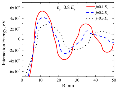
Figure 1: (Color online) Indirect exchange interaction energy vs distance between ions in the resonant case

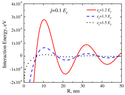
Figure 2: (Color online) Indirect exchange interaction energy vs distance between ions in the non-resonant case

In our calculation we have obtained the interaction energy by analyzing the phase shift for scattering at the impurity potential and its effect on the density of states for the standing waves in a box. This approach, which has been never applied to the indirect exchange problem before, allowed us to analyze the resonant case. For the bound state energy being within the energy range occupied by the free carriers the indirect exchange interaction appears to be much stronger than expected from the RKKY approach. We believe that the new results may shed the light on ferromagnetic coupling in Mn layers in InGaAs-based heterostructures and other nanostructures with paramagnetic impurities.

The work has been supported by RFBR (grants no 11-02-00348, 11-02-00146, 12-02-00815, 12-02-00141), RF President Grant NSh-5442.2012.2, Dynasty Foundation.

References

Korenev et al. (2012)
V. Korenev,
I. Akimov,
S. Zaitsev,
V. Sapega,
L. Langer,
D. Yakovlev,
Y. A. Danilov,
and M. Bayer,
Nat. Commun. 3,
959 (2012).
Zaitsev et al. (2010)
S. Zaitsev,
M. Dorokhin,
A. Brichkin,
O. Vikhrova,
Y. Danilov,
B. Zvonkov, and
V. Kulakovskii,
JETP Letters 90,
658 (2010).
Jungwirth et al. (2006)
T. Jungwirth,
J. Sinova,
J. Mašek,
J. Kučera, and A. H.
MacDonald, Rev. Mod. Phys.
78, 809 (2006).
Tripathi et al. (2011)
V. Tripathi,
K. Dhochak,
B. A. Aronzon,
V. V. Rylkov,
A. B. Davydov,
B. Raquet,
M. Goiran, and
K. I. Kugel,
Phys. Rev. B 84,
075305 (2011).
Ruderman and Kittel (1954)
M. A. Ruderman and
C. Kittel,
Phys. Rev. 96,
99 (1954).
Fano (1961)
U. Fano, Phys.
Rev. 124, 1866
(1961).
Rozhansky et al. (2012)
I. V. Rozhansky,
N. S. Averkiev,
and
E. Lähderanta,
Phys. Rev. B 85,
075315 (2012).
Bardeen (1961)
J. Bardeen,
Phys. Rev. Lett. 6,
57 (1961).
Rozhansky et al. (2013)
I. V. Rozhansky,
N. S. Averkiev,
and
E. Lähderanta,
Low Temperature Physics 39,
28 (2013).