Error Analysis of Semidiscrete Finite Element Methods for Inhomogeneous Time-Fractional Diffusion

Abstract.

We consider the initial boundary value problem for the inhomogeneous time-fractional diffusion equation with a homogeneous Dirichlet boundary condition and a nonsmooth right hand side data in a bounded convex polyhedral domain. We analyze two semidiscrete schemes based on the standard Galerkin and lumped mass finite element methods. Almost optimal error estimates are obtained for right hand side data $f(x,t)\in L^{\infty}(0,T;\dot{H}^{q}(\Omega))$, $-1<q\leq 1$, for both semidiscrete schemes. For lumped mass method, the optimal $L^{2}(\Omega)$-norm error estimate requires symmetric meshes. Finally, numerical experiments for one- and two-dimensional examples are presented to verify our theoretical results.

1. Introduction

We consider the model initial-boundary value problem for the fractional-order parabolic differential equation (FPDE) for $u(x,t)$:

$${\partial^{\alpha}_{t}}u-\Delta u =f, \quad\text{in }\Omega \quad T\geq t>0,$$

(1.1) $$u =0, \quad\text{on}\ \partial\Omega \quad T\geq t>0,$$

$$u(0) =v, \quad\text{in }\Omega,$$

where $\Omega$ is a bounded convex polygonal domain in $\mathbb{R}^{d}\,(d=1,2,3)$ with a boundary $\partial\Omega$, $v$ and $f$ are given functions and $T>0$ is a fixed value. In the model (1), ${\partial^{\alpha}_{t}}u$ refers to the Caputo fractional derivative of order $\alpha$ ($0<\alpha<1$) of the function $u(t)$, and it is defined by [12, pp. 91, eq. (2.4.1)]

$${\partial^{\alpha}_{t}}u(t)=\frac{1}{\Gamma(1-\alpha)}\int_{0}^{t}\frac{1}{(t-s)^{\alpha}}u^{\prime}(s)ds.$$

It is known that for the fractional order $\alpha=1$, the fractional derivative ${\partial^{\alpha}_{t}}u$ recovers the canonical first-order derivative $u^{\prime}(t)$ [12, pp. 92, eq. (2.4.14)], and accordingly the model (1) reduces to the classical time-dependent diffusion problem. Therefore, the model (1) can be regarded as a fractional counterpart of the standard diffusion problem.

The interest in (1) is mainly motivated by anomalous diffusion processes, known as subdiffusion, in which the mean square variance grows slower than that in a Gaussian process. At a microscopic level, the diffusion process results from random motion of particles. In a subdiffusion process, the waiting time between consecutive random particle motion can be very large, and thus the mean waiting time diverges. Thus, the underlying stochastic process deviates significantly from the Brownian motion, and instead it can only be more adequately described by the continuous time random walk (CTRW) [17]. This microscopic explanation has been frequently exploited in applications. For example, Adams and Gelhar [1] observed that field data show anomalous diffusion in a highly heterogeneous aquifer, and Hatano and Hatano [7] applied the CTRW to model anomalous diffusion in an underground environmental problem. The macroscopic counterpart of the CTRW is a diffusion equation with a time fractional derivative ${\partial^{\alpha}_{t}}u(t)$, i.e. model (1). It has been successfully applied to many practical problems, including diffusion in media with fractal geometry [19], the dynamics of viscoelastic materials [6], and contaminant transport within underground water flow [3].

The modeling capabilities of FPDEs have generated considerable interest in deriving, analyzing, and testing numerical methods for such problems. As a result, a number of numerical techniques were developed, and their stability and convergence properties were investigated. Yuste and Acedo [25] presented a numerical scheme by combining the forward time centered space method for the ordinary diffusion equation and Grunwald-Letnikov discretization of the (Riemann-Liouville type) fractional-derivative and provided a von Neumann type stability analysis. Lin and Xu [14] proposed a numerical method based a finite difference scheme in time and Legendre spectral method in space, showed its unconditional stability, and provided error estimates. Li and Xu [13] developed a spectral method in both temporal and spatial variables and established various a priori error estimates. Mustapha [18] studied semidiscrete in time and fully discrete schemes and derived error bounds for smooth initial data [18, Theorem 4.3]. In all these useful studies, the error analysis was carried out under the assumption that the solution is sufficiently smooth. The optimality of the estimates with respect to the solution smoothness expressed through the problem data, i.e., the right hand side $f$ and the initial data $v$, was not considered.

Thus, these useful studies do not cover the interesting case of solutions with limited regularity due to low regularity of the data, a typical case for related inverse problems; see, e.g., [5] and also [11] and [24] for its parabolic counterpart. In our earlier work [9], we have analyzed the semidiscrete Galerkin finite element method (FEM) and lumped mass method for problem (1) with a zero right hand side. In particular, almost optimal error estimates were established for both smooth and nonsmooth initial data, i.e., $v\in\dot{H}^{q}(\Omega)$, $0\leq q\leq 1$. (See section 2.2 for the definitions of the space $\dot{H}^{q}(\Omega)$.) More recently in [8], the results were generalized to the case of very weak initial data, i.e., $v\in\dot{H}^{q}(\Omega)$, $-1<q<0$ . We also refer interested readers to [15, 16] for related studies on FPDEs with a Riemann-Liouville fractional derivative and non-smooth initial data.

In this work, we analyze the case of a non-smooth right hand side, i.e., $f\in L^{r}(0,T;\dot{H}^{q}(\Omega))$, $-1<q\leq 1$, $r>1$. Such problems occur in many practical applications, e.g., optimal control problems and inverse problems [10]. Thus, it is of immense interest to develop and to analyze related numerical schemes. However, with such weak data it might be difficult to define a proper weak solution. In Remark 2.2 below, we note that a function $u(x,t)$ expressed by the representation (2.4) satisfies the differential equation for $1<r$, but it satisfies (in generalized sense) the initial condition $u(x,0)=0$ for $r>1/\alpha$ only. Therefore, the natural class of weak data would be $f\in L^{r}(0,T;\dot{H}^{q}(\Omega))$, $-1<q\leq 1$, $r>1/\alpha$. In fact, all results (upon minor modifications) in this paper are valid for problem (1) with such data. However, for the ease of exposition, we shall assume that $f\in L^{\infty}(0,T;\dot{H}^{q}(\Omega))$, $-1<q\leq 1$, which guarantees that the representation formula (2.4) does give a legitimate solution weak solution $u(x,t)$ for all $0<\alpha<1$.

The goal of this paper is to develop an error analysis with optimal with respect to the regularity of the right hand side estimates for the semidiscrete Galerkin and the lumped mass Galerkin FEM for problem (1) on convex polygonal domains. Now we describe the numerical schemes, using the standard notation from [23]. Let $\{\mathcal{T}_{h}\}$, $0<h<1$, be a family of shape regular and quasi-uniform partitions of the domain $\Omega$ into $d$-simplices, called finite elements, with $h$ denoting the maximum diameter. The approximate solution $u_{h}$ will be sought in the finite element space $X_{h}=X_{h}(\Omega)$ of continuous piecewise linear functions over the triangulation $\mathcal{T}_{h}$

$$X_{h}=\{\chi\in H_{0}^{1}(\Omega):\chi\mbox{ is a linear function over }\tau\quad\forall\tau\in\mathcal{T}_{h}\}.$$

The semidiscrete Galerkin FEM for problem (1) reads: find $u_{h}(t)\in X_{h}$ such that

$$({\partial^{\alpha}_{t}}u_{h}(t),\chi)+a(u_{h},\chi)=(f,\chi),\quad\forall\chi\in X_{h},\ \ t>0,$$

with $u_{h}(0)=0$, and $a(u,w)=(\nabla u,\nabla w)$ for $u,w\in H_{0}^{1}(\Omega)$. We shall study the convergence of the semidiscrete Galerkin FEM for the case of a right hand side $f\in L^{\infty}(0,T;\dot{H}^{q}(\Omega))$, $-1<q\leq 1$.

The main difficulty in the analysis stems from limited smoothing properties of the solution operator, cf. Lemma 2.2. This difficulty is overcome by exploiting the mapping property of discrete solution operators established in Lemma 3.2. Our main results are as follows. First in Theorem 3.1, we derive an optimal $L^{2}(0,T;\dot{H}^{p}(\Omega))$-norm, $p=0,1$, error bound:

$$\|u_{h}-u\|_{L^{2}(0,T;L^{2}(\Omega))}+h\|\nabla(u_{h}-u)\|_{L^{2}(0,T;L^{2}(\Omega))}\leq Ch^{2+\min(q,0)}\|f\|_{L^{2}(0,T;\dot{H}^{q}(\Omega))},$$

for $-1<q\leq 1$. Second, we derive an almost optimal $L^{\infty}(0,T;\dot{H}^{p}(\Omega))$-norm estimate of the error with an additional log-factor $\ell_{h}:=|\ln h|$ for $f\in L^{\infty}(0,T;\dot{H}^{q}(\Omega))$, $-1<q\leq 1$ (cf. Theorem 3.2):

$$\|u_{h}(t)-u(t)\|_{L^{2}(\Omega)}+h\|\nabla(u_{h}(t)-u(t))\|_{L^{2}(\Omega)}\leq Ch^{2+\min(q,0)}\,\ell_{h}^{2}\|f\|_{L^{\infty}(0,t;\dot{H}^{q}(\Omega))}.$$

Further, we study the more practical lumped mass scheme, and show the same convergence rates for the gradient. For right hand side $f\in L^{\infty}(0,T;\dot{H}^{q}(\Omega))$, $-1<q<1$, on general quasi-uniform meshes, we are only able to establish a suboptimal $L^{2}$-error bound of order $O(h^{1+q}\ell_{h}^{2})$. For a class of special triangulations satisfying condition (4.11), (almost) optimal estimates of order $O(h^{2+\min(q,0)})$ and $O(h^{2+\min(q,0)}\ell_{h}^{2})$ hold in $L^{2}(0,T;L^{2}(\Omega))$- and $L^{\infty}(0,T;L^{2}(\Omega))$-norm, respectively, cf. Theorems 4.2 and 4.4. These results extend related results for nonsmooth initial data obtained in our earlier works [8, 9].

The rest of the paper is organized as follows. In Section 2, we recall some preliminaries for the convergence analysis, including basic properties of the Mittag-Leffler function, the smoothing property of (1), and basic estimates for finite element projection operators. In Sections 3 and 4, we derive error estimates for the standard Galerkin FEM and lumped mass FEM, respectively. Finally, in Section 5 we present numerical results for both one- and two-dimensional examples, including non-smooth and very weak data, which confirm our theoretical study. Throughout, we shall denote by $C$ a generic constant, which may differ at different occurrences and may depend on $T$, but it is always independent of the solution $u$ and the mesh size $h$.

2. preliminaries

In this part, we recall preliminaries for the convergence analysis, including the Mittag-Leffler function, solution representation, stability estimates, and basic properties of the finite element projection operators.

2.1. Mittag-Leffler function

The Mittag-Leffler function $E_{\alpha,\beta}(z)$ is defined by

$$E_{\alpha,\beta}(z)=\sum_{k=0}^{\infty}\frac{z^{k}}{\Gamma(k\alpha+\beta)}\quad z\in\mathbb{C}\quad\mbox{with}\quad\Gamma(z)=\int_{0}^{\infty}t^{z-1}e^{-t}dt\,\quad~{}~{}\Re(z)>0.$$

The function $E_{\alpha,\beta}(z)$ generalizes the exponential function in that $E_{1,1}(z)=e^{z}$. The variant $E_{\alpha,\alpha}(z)$, appears in the kernel of the solution representation of problem (1); see (2.3) and (2.4) below. The following properties are essential in our analysis.

Lemma 2.1.

Let $0<\alpha<2$ and $\beta\in\mathbb{R}$ be arbitrary, and $\frac{\alpha\pi}{2}<\mu<\min(\pi,\alpha\pi)$. Then there exists a constant $C=C(\alpha,\beta,\mu)>0$ such that for $\mu\leq|\mathrm{arg}(z)|\leq\pi$

(2.1) $$|E_{\alpha,\beta}(z)|\leq\left\{\begin{aligned} \frac{C}{1+|z|^{2}},&\quad\beta-\alpha\in\mathbb{Z}^{-}\cup\{0\},\\ \frac{C}{1+|z|},&\quad\mbox{otherwise}.\end{aligned}\right.$$

Moreover, for $\lambda>0$, $\alpha>0$, and $t>0$ we have

(2.2) $${\partial^{\alpha}_{t}}E_{\alpha,1}(-\lambda t^{\alpha}) =-\lambda E_{\alpha,1}(-\lambda t^{\alpha})\quad\mbox{and}\quad\frac{d}{dt}E_{\alpha,1}(-\lambda t^{\alpha})=-\lambda t^{\alpha-1}E_{\alpha.\alpha}(-\lambda t^{\alpha}).$$

Proof.

The estimate (2.1) can be found in [12, pp. 43, equation (1.8.28)] or [20, Theorem 1.4], while (2.2) is discussed in [12, Lemma 2.33, equations (2.4.58) and (1.10.7)]. ∎

2.2. Solution representation

For the solution representation to problem (1), we first introduce some notation. For $s\geq-1$, we denote by $\dot{H}^{s}(\Omega)\subset H^{-1}(\Omega)$ the Hilbert space induced by the norm:

$$\|v\|_{\dot{H}^{s}(\Omega)}^{2}=\sum_{j=1}^{\infty}\lambda_{j}^{s}\langle v,\varphi_{j}\rangle^{2}$$

with $\{\lambda_{j}\}_{j=1}^{\infty}$ and $\{\varphi_{j}\}_{j=1}^{\infty}$ being respectively the eigenvalues and the $L^{2}(\Omega)$-orthonormal eigenfunctions of the Laplace operator $-\Delta$ on the domain $\Omega$ with a homogeneous Dirichlet boundary condition. As usual, we identify a function $f$ in $L^{2}(\Omega)$ with the functional $F$ in $H^{-1}(\Omega)$ defined by $\langle F,\phi\rangle=(f,\phi)$, for all $\phi\in H^{1}_{0}(\Omega)$. Then $\{\varphi_{j}\}_{j=1}^{\infty}$ and $\{\lambda_{j}^{1/2}\varphi_{j}\}_{j=1}^{\infty}$, form orthonormal basis in $L^{2}(\Omega)$ and $H^{-1}(\Omega)$, respectively. Further, $\|v\|_{\dot{H}^{0}(\Omega)}=\|v\|_{L^{2}(\Omega)}=(v,v)^{1/2}$ is the norm in $L^{2}(\Omega)$ and $\|v\|_{\dot{H}^{-1}(\Omega)}=\|v\|_{H^{-1}(\Omega)}$ is the norm in $H^{-1}(\Omega)$. Besides, it is easy to verify that $\|v\|_{\dot{H}^{1}(\Omega)}=\|\nabla v\|_{L^{2}(\Omega)}$ is also the norm in $H_{0}^{1}(\Omega)$ and $\|v\|_{\dot{H}^{2}(\Omega)}=\|\Delta v\|_{L^{2}(\Omega)}$ is equivalent to the norm in $H^{2}(\Omega)\cap H^{1}_{0}(\Omega)$ (cf. the proof of Lemma 3.1 of [23]). Note that $\dot{H}^{s}(\Omega)$, $s\geq-1$ form a Hilbert scale of interpolation spaces. Motivated by this, we denote $\|\cdot\|_{H^{s}(\Omega)}$ to be the norm on the interpolation scale between $H^{1}_{0}(\Omega)$ and $L^{2}(\Omega)$ when $s$ is in $[0,1]$ and $\|\cdot\|_{H^{s}(\Omega)}$ to be the norm on the interpolation scale between $L^{2}(\Omega)$ and $H^{-1}(\Omega)$ when $s$ is in $[-1,0]$. Then, $\|\cdot\|_{H^{s}(\Omega)}$ and $\|\cdot\|_{\dot{H}^{s}(\Omega)}$ are equivalent for $s\in[-1,1]$ by interpolation.

For a Banach space $B$, we define the space

$$L^{r}(0,T;B)=\{u(t)\in B\mbox{ for a.e. }t\in(0,T)\mbox{ and }\|u\|_{L^{r}(0,T;B)}<\infty\},$$

for any $r\geq 1$, and the norm $\|\cdot\|_{L^{r}(0,T;B)}$ is defined by

$$\|u\|_{L^{r}(0,T;B)}=\left\{\begin{aligned} \left(\int_{0}^{T}\|u(t)\|_{B}^{r}dt\right)^{1/r},&\quad r\in[1,\infty),\\ \mathrm{esssup}_{t\in(0,T)}\|u(t)\|_{B},&\quad r=\infty.\end{aligned}\right.$$

Now we give a representation of the solution to problem (1) using the eigenpairs $\{(\lambda_{j},\varphi_{j})\}_{j=1}^{\infty}$. We define an operator $\bar{E}(t)$ for $\chi\in L^{2}(\Omega)$ by

(2.3) $${\bar{E}}(t)\chi=\sum_{j=1}^{\infty}t^{\alpha-1}{E_{\alpha,\alpha}}(-\lambda_{j}t^{\alpha})\,(\chi,\varphi_{j})\,\varphi_{j}(x).$$

Then by separation of variables we get the following representation of the solution $u(x,t)$ to problem (1) for initial data $v=0$:

(2.4) $$u(x,t)=\int_{0}^{t}{\bar{E}}(t-s)f(s)ds.$$

Our first task is to find the weakest class of right hand side data $f(x,t)$ so that (2.4) is indeed a solution to the problem (1). As we see below, for any $f\in L^{2}(0,T;\dot{H}^{s}(\Omega))$, $-1<s\leq 1$ the function $u(x,t)$ from (2.4) satisfies the differential equation as an element in the space $L^{2}(0,T;\dot{H}^{s+2}(\Omega))$. However, it may not satisfy the homogeneous initial condition $u(x,0)=0$. In Remark 2.2 we argue that the weakest class of source term that produces a legitimate weak solution of (1) is $f\in L^{r}(0,T;\dot{H}^{s}(\Omega))$ with $r>1/\alpha$ and $-1<s\leq 1$. Obviously, for $1/2<\alpha<1$, the representation (2.4) does give a solution $u(x,t)\in L^{2}(0,T;\dot{H}^{s+2}(\Omega))$.

We begin with the following important smoothing property of the solution operator $\bar{E}$.

Lemma 2.2.

For any $t>0$, we have for $0\leq p-q\leq 4$

$$\|\bar{E}(t)\chi\|_{\dot{H}^{p}(\Omega)}\leq Ct^{-1+\alpha(1+(q-p)/2)}\|\chi\|_{\dot{H}^{q}(\Omega)}.$$

Proof.

The definition of $\bar{E}$ in (2.3) and Lemma 2.1 yield

$$\begin{split}\|\bar{E}(t)\chi\|_{\dot{H}^{p}(\Omega)}^{2}&=\sum_{j=1}^{\infty}\lambda_{j}^{p}|t^{\alpha-1}{E_{\alpha,\alpha}}(-\lambda_{j}t^{\alpha})|^{2}|(\chi,\varphi_{j})|^{2}\\ &=t^{-2+(2+q-p)\alpha}\sum_{j=1}^{\infty}(\lambda_{j}t^{\alpha})^{p-q}|{E_{\alpha,\alpha}}(-\lambda_{j}t^{\alpha})|^{2}\lambda_{j}^{q}|(\chi,\varphi_{j})|^{2}\\ &\leq Ct^{-2+(2+q-p)\alpha}\sum_{j=1}^{\infty}\frac{(\lambda_{j}t^{\alpha})^{p-q}}{(1+(\lambda_{j}t^{\alpha})^{2})^{2}}\lambda_{j}^{q}|(\chi,\varphi_{j})|^{2}\\ &\leq Ct^{-2+(2+q-p)\alpha}\sum_{j=1}^{\infty}\lambda_{j}^{q}|(\chi,\varphi_{j})|^{2}\leq Ct^{-2+(2+q-p)\alpha}\|\chi\|_{\dot{H}^{q}(\Omega)},\end{split}$$

where in the last line we have used the inequality $\sup_{j}\frac{(\lambda_{j}t^{\alpha})^{p-q}}{(1+(\lambda_{j}t^{\alpha})^{2})^{2}}\leq C$ for $0\leq p-q\leq 4$. From this inequality the desired estimate follows immediately. ∎

Next we state some stability estimates for the solution $u$ to problem (1) for $f\in L^{\infty}(0,T;\dot{H}^{q}(\Omega))$, $-1<q\leq 1$. These estimates will be essential for the convergence analysis of the standard Galerkin FEM in Section 3. The first estimate in Theorem 2.1 in the case $q=0$ was already established in [21, Theorem 2.1, part (i)]. Below it is extended for the whole range of $q$.

Theorem 2.1.

Assume that $f\in L^{2}(0,T;\dot{H}^{q}(\Omega))$, $-1<q\leq 1$. Then the expression (2.4) represents a function $u\in L^{2}(0,T;\dot{H}^{q+2}(\Omega))$ which satisfies the differential equation in (1) and the estimate:

(2.5) $$\|u\|_{L^{2}(0,T;\dot{H}^{q+2}(\Omega))}+\|\partial_{t}^{\alpha}u\|_{L^{2}(0,T;\dot{H}^{q}(\Omega))}\leq C\|f\|_{L^{2}(0,T;\dot{H}^{q}(\Omega))}.$$

If $f\in L^{\infty}(0,T;\dot{H}^{q}(\Omega))$, $-1<q\leq 1$, then the function $u(x,t)$ belongs to $L^{\infty}(0,T;\dot{H}^{q+2-\epsilon}(\Omega))$ and satisfies

(2.6) $$\|u(\cdot,t)\|_{\dot{H}^{q+2-\epsilon}(\Omega)}\leq C\epsilon^{-1}t^{\epsilon\alpha/2}\|f\|_{L^{\infty}(0,t;\dot{H}^{q}(\Omega))}\quad\mbox{ for any}\quad\epsilon>0.$$

Hence, (2.4) is a solution to the initial value problem (1) with a homogeneous initial data $v=0$.

Proof.

By the complete monotonicity of the function $E_{\alpha,1}(-t^{\alpha})$ (with $\alpha\in(0,1)$) [21, Lemma 3.3], i.e.,

$$(-1)^{n}\frac{d^{n}}{dt^{n}}E_{\alpha,1}(-t^{\alpha})\geq 0\quad\mbox{ for all }t>0,\ \ n=0,1,\ldots,$$

and the differentiation formula in Lemma 2.1, we deduce $E_{\alpha,\alpha}(-\eta)\geq 0$, $\eta\geq 0$. Therefore, for $t>0$

(2.7) $$\int_{0}^{t}|t^{\alpha-1}E_{\alpha,\alpha}(-\lambda_{n}t^{\alpha})|dt =\int_{0}^{t}t^{\alpha-1}E_{\alpha,\alpha}(-\lambda_{n}t^{\alpha})dt$$

$$=-\frac{1}{\lambda_{n}}\int_{0}^{t}\frac{d}{dt}E_{\alpha,1}(-\lambda_{n}t^{\alpha})dt$$

$$=\frac{1}{\lambda_{n}}(1-E_{\alpha,1}(-\lambda_{n}t^{\alpha}))\leq\frac{1}{\lambda_{n}}.$$

Meanwhile, by the differentiation formula [12, pp. 140-141], we get

$$A_{n}:= \partial_{t}^{\alpha}\int_{0}^{t}(f(\cdot,\tau),\varphi_{n})(t-\tau)^{\alpha-1}E_{\alpha,\alpha}(-\lambda_{n}(t-\tau)^{\alpha})d\tau$$

$$= (f(\cdot,t),\varphi_{n})-\lambda_{n}\int_{0}^{t}(f(\cdot,\tau),\varphi_{n})(t-\tau)^{\alpha-1}E_{\alpha,\alpha}(-\lambda_{n}(t-\tau)^{\alpha})d\tau.$$

Now by means of Young’s inequality for convolution, we deduce

$$\|A_{n}\|_{L^{2}(0,T)}^{2} \leq C_{1}\int_{0}^{T}|(f(\cdot,t),\varphi_{n})|^{2}dt+C_{2}\int_{0}^{T}|(f(\cdot,t),\varphi_{n})|^{2}dt\left(\int_{0}^{T}|\lambda_{n}t^{\alpha-1}E_{\alpha,\alpha}(-\lambda_{n}t^{\alpha})|dt\right)^{2}$$

$$\leq C\int_{0}^{T}|(f(\cdot,t),\varphi_{n})|^{2}\,dt.$$

Thus there holds

$$\|\partial_{t}^{\alpha}u\|_{L^{2}(0,T;\dot{H}^{q}(\Omega))}^{2} =\sum_{n=1}^{\infty}\int_{0}^{T}\lambda_{n}^{q}|\partial_{t}^{\alpha}\int_{0}^{t}(f(\cdot,\tau),\varphi_{n})(t-\tau)^{\alpha-1}E_{\alpha,\alpha}(-\lambda_{n}(t-\tau)^{\alpha})d\tau|^{2}dt$$

$$\leq C\sum_{n=1}^{\infty}\int_{0}^{T}\lambda_{n}^{q}|(f(\cdot,t),\phi_{n})|^{2}dt=C\|f\|_{L^{2}(0,T;\dot{H}^{q}(\Omega))}^{2}.$$

Now using equation (1) and the triangle inequality, we also get $\|\Delta u\|_{L^{2}(0,T;\dot{H}^{q}(\Omega))}\leq C\|f\|_{L^{2}(0,T;\dot{H}^{q}(\Omega))}$. This shows the first assertion. By Lemma 2.2 we have

$$\|u(\cdot,t)\|_{\dot{H}^{q+2-\epsilon}(\Omega)} =\|\int_{0}^{t}\bar{E}(t-s)f(s)ds\|_{\dot{H}^{q+2-\epsilon}(\Omega)}\leq\int_{0}^{t}\|\bar{E}(t-s)f(s)\|_{\dot{H}^{q+2-\epsilon}(\Omega)}ds$$

$$\leq C\int_{0}^{t}(t-s)^{\epsilon\alpha/2-1}\|f(s)\|_{\dot{H}^{q}(\Omega)}ds\leq C\epsilon^{-1}t^{\epsilon\alpha/2}\|f\|_{L^{\infty}(0,t;\dot{H}^{q}(\Omega))}$$

which shows estimate (2.6). Finally, it is follows directly from this that the representation $u$ satisfies also the initial condition $u(0)=0$, i.e., for any $\epsilon>0$, $\lim_{t\to 0}\|u(\cdot,t)\|_{\dot{H}^{q+2-\epsilon}(\Omega)}=0$, and thus it is indeed a solution of the initial value problem (1). ∎

Remark 2.1.

The first estimate in Theorem 2.1 can be improved to

$$\|u\|_{L^{r}(0,T;\dot{H}^{q+2}(\Omega))}+\|\partial_{t}^{\alpha}u\|_{L^{r}(0,T;\dot{H}^{q})}\leq C\|f\|_{L^{r}(0,T;\dot{H}^{q}(\Omega))}$$

for any $r\in(1,\infty)$. The proof is essentially identical. The $\epsilon$ factor in the second estimate reflects the limited smoothing property of the fractional differential operator, resulting from the slow decay of the Mittag-Leffler function $E_{\alpha,\alpha}(-z)$.

Remark 2.2.

The condition $f\in L^{\infty}(0,T;\dot{H}^{q}(\Omega))$ can be weakened to $f\in L^{r}(0,T;\dot{H}^{q}(\Omega))$ with $r>1/\alpha$. This follows from Lemma 2.2 and the Cauchy-Schwarz inequality with $r^{\prime}$, $1/r^{\prime}+1/r=1$

$$\|u(\cdot,t)\|_{\dot{H}^{q}(\Omega)} \leq\int_{0}^{t}\|\bar{E}(t-s)f(s)\|_{\dot{H}^{q}(\Omega)}ds\leq\int_{0}^{t}(t-s)^{\alpha-1}\|f(s)\|_{\dot{H}^{q}(\Omega)}ds$$

$$\leq\tfrac{C}{1+r^{\prime}(\alpha-1)}t^{1+r^{\prime}(\alpha-1)}\|f\|_{L^{r}(0,t;\dot{H}^{q}(\Omega))},$$

where $1+r^{\prime}(\alpha-1)>0$ by the condition $r>1/\alpha$. It follows from this that the initial condition $u(x,0)=0$ holds in the following sense: $\lim_{t\to 0^{+}}\|u(t)\|_{\dot{H}^{q}(\Omega)}=0$. Hence for any $\alpha\in(1/2,1)$ the representation formula (2.4) remains a legitimate solution under the weaker condition $f\in L^{2}(0,T;\dot{H}^{q}(\Omega))$.

Remark 2.3.

For the ease of exposition, in the error analysis we shall restrict our discussion to the case $f\in L^{\infty}(0,T;\dot{H}^{q}(\Omega))$. Nonetheless, we note that for $p=0,1$ the $L^{2}(0,T;\dot{H}^{p}(\Omega))$-norm estimate of the error below remain valid under the weakened regularity condition on the source term $f$.

2.3. Ritz and $L^{2}$-orthogonal projections

In our analysis we shall also use the $L^{2}$-orthogonal projection $P_{h}:L^{2}(\Omega)\to X_{h}$ and the Ritz projection $R_{h}:H^{1}_{0}(\Omega)\to X_{h}$, respectively, defined by

$$(P_{h}\psi,\chi) =(\psi,\chi)\quad\forall\chi\in X_{h},$$

$$(\nabla R_{h}\psi,\nabla\chi) =(\nabla\psi,\nabla\chi)\quad\forall\chi\in X_{h}.$$

We shall need some properties of the Ritz projection $R_{h}$ and the $L^{2}$-projection $P_{h}$ [8].

Lemma 2.3.

Let the mesh be quasi-uniform. Then the operator $R_{h}$ satisfies:

$$\|R_{h}\psi-\psi\|_{L^{2}(\Omega)}+h\|\nabla(R_{h}\psi-\psi)\|_{L^{2}(\Omega)}\leq Ch^{q}\|\psi\|_{\dot{H}^{q}(\Omega)}\quad{\mbox{for}}\quad\psi\in\dot{H}^{q}(\Omega),\ q=1,2.$$

Further, for $s\in[0,1]$ we have

$$\|(I-P_{h})\psi\|_{H^{s}(\Omega)} \leq Ch^{2-s}\|\psi\|_{\dot{H}^{2}(\Omega)}\quad{\mbox{for}}\quad\psi\in H^{2}(\Omega)\cap H^{1}_{0}(\Omega),$$

$$\|(I-P_{h})\psi\|_{H^{s}(\Omega)} \leq Ch^{1-s}\|\psi\|_{\dot{H}^{1}(\Omega)}\quad{\mbox{for}}\quad\psi\in H^{1}_{0}(\Omega).$$

In addition, by duality $P_{h}$ is stable on $\dot{H}^{s}(\Omega)$ for $s\in[-1,0]$.

3. Semidiscrete Galerkin FEM

3.1. Finite element method

The semidiscrete Galerkin FEM for problem (1) with $v=0$ is: find $u_{h}\in X_{h}$ such that

(3.1) $$\begin{split}{({\partial^{\alpha}_{t}}u_{h},\chi)}+a(u_{h},\chi)&={(f,\chi)},\quad\forall\chi\in X_{h},\ T\geq t>0\quad\mbox{and}\quad u_{h}(0)=0.\end{split}$$

Upon introducing the discrete Laplace operator $\Delta_{h}:X_{h}\to X_{h}$

(3.2) $$-(\Delta_{h}\psi,\chi)=(\nabla\psi,\nabla\chi)\quad\forall\psi,\,\chi\in X_{h},$$

the spatial discrete problem can be written as

(3.3) $${\partial^{\alpha}_{t}}u_{h}(t)-\Delta_{h}u_{h}(t)=f_{h}(t)\quad{\mbox{for}}\quad t\geq 0\quad\mbox{with}\quad u_{h}(0)=0,$$

where the discrete source term $f_{h}=P_{h}f$. Then the solution of (3.3) can be represented by the eigenpairs $\{(\lambda^{h}_{j},\varphi_{j}^{h})\}_{j=1}^{{N}}$ of the discrete Laplacian $-\Delta_{h}$. Now we introduce the discrete analogue $\bar{E}_{h}$ of the solution operator $\bar{E}$ defined in (2.3) for $t>0$:

(3.4) $${\bar{E}_{h}}(t)f_{h}=\sum_{j=1}^{N}t^{\alpha-1}{E_{\alpha,\alpha}}(-\lambda^{h}_{j}t^{\alpha})\,(f_{h},\varphi^{h}_{j})\,\varphi_{j}^{h}.$$

Then the solution $u_{h}(x,t)$ of the discrete problem (3.3) can be expressed by:

(3.5) $$u_{h}(x,t)=\int_{0}^{t}{\bar{E}_{h}}(t-s)f_{h}(s)\,ds.$$

Now we define the discrete norm $|\thickspace\!\!|\thickspace\!\!|\cdot|\thickspace\!\!|\thickspace\!\!|_{\dot{H}^{p}(\Omega)}$ on $X_{h}$ for any $p\in\mathbb{R}$

(3.6) $$|\thickspace\!\!|\thickspace\!\!|\psi|\thickspace\!\!|\thickspace\!\!|_{\dot{H}^{p}(\Omega)}^{2}=\sum_{j=1}^{N}(\lambda_{j}^{h})^{p}(\psi,\varphi_{j}^{h})^{2}\quad\psi\in X_{h}.$$

Analogously, we introduce the associated spaces $|\thickspace\!\!|\thickspace\!\!|\cdot|\thickspace\!\!|\thickspace\!\!|_{L^{r}(0,T;\dot{H}^{p}(\Omega))}$, $r\in[1,\infty]$, on the space $X_{h}$.

We have the following norm equivalence and inverse inequality.

Lemma 3.1.

For all $\psi\in X_{h}$ and any real $l>s$

$$|\thickspace\!\!|\thickspace\!\!|\psi|\thickspace\!\!|\thickspace\!\!|_{\dot{H}^{l}(\Omega)}\leq Ch^{s-l}|\thickspace\!\!|\thickspace\!\!|\psi|\thickspace\!\!|\thickspace\!\!|_{\dot{H}^{s}(\Omega)}.$$

For any $s\in[-1,1]$, the norms $|\thickspace\!\!|\thickspace\!\!|\cdot|\thickspace\!\!|\thickspace\!\!|_{\dot{H}^{s}(\Omega)}$ and $\|\cdot\|_{\dot{H}^{s}(\Omega)}$ are equivalent on $X_{h}$.

Proof.

The inverse estimate was shown in [9, Lemma 3.3]. By the definition of the $|\thickspace\!\!|\thickspace\!\!|\cdot|\thickspace\!\!|\thickspace\!\!|_{\dot{H}^{s}(\Omega)}$-norm and the discrete Laplace operator, it is easy to show $|\thickspace\!\!|\thickspace\!\!|\cdot|\thickspace\!\!|\thickspace\!\!|_{\dot{H}^{s}(\Omega)}$ is equivalent to $\|\cdot\|_{\dot{H}^{s}(\Omega)}$ with $s=0,1$. Then the assertion for $0\leq s\leq 1$ follows by interpolation, and by duality it is also equivalent to $\|\cdot\|_{\dot{H}^{s}(\Omega)}$ for $-1\leq s\leq 0$. ∎

3.2. Properties of the discrete solution

Next, analogous to Lemma 2.2, we introduce some smoothing properties of ${\bar{E}_{h}}(t)$. The proof is identical with that for Lemma 2.2, and hence omitted.

Lemma 3.2.

Let ${\bar{E}_{h}}$ be defined by (3.4) and $\psi\in X_{h}$. Then we have for all $t>0$,

$$|\thickspace\!\!|\thickspace\!\!|{\bar{E}_{h}}(t)\psi|\thickspace\!\!|\thickspace\!\!|_{\dot{H}^{p}(\Omega)}\leq\left\{\begin{array}[]{ll}Ct^{-1+\alpha(1+(q-p)/2)}|\thickspace\!\!|\thickspace\!\!|\psi|\thickspace\!\!|\thickspace\!\!|_{\dot{H}^{q}(\Omega)},&\quad p-4\leq q\leq p,\\[5.59721pt] Ct^{-1+\alpha}|\thickspace\!\!|\thickspace\!\!|\psi|\thickspace\!\!|\thickspace\!\!|_{\dot{H}^{q}(\Omega)},&\quad p<q.\end{array}\right.$$

The following estimate is the discrete analogue of Theorem 2.1. It is essential for the analysis of the lumped mass method in Section 4.

Lemma 3.3.

Let $u_{h}$ be the solution of (3.3). Then for arbitrary $p>-1$

(3.7) $$\int_{0}^{T}|\thickspace\!\!|\thickspace\!\!|{\partial^{\alpha}_{t}}u_{h}(t)|\thickspace\!\!|\thickspace\!\!|_{\dot{H}^{p}(\Omega)}^{2}+|\thickspace\!\!|\thickspace\!\!|u_{h}(t)|\thickspace\!\!|\thickspace\!\!|_{\dot{H}^{p+2}(\Omega)}^{2}\,dt \leq\int_{0}^{T}|\thickspace\!\!|\thickspace\!\!|f_{h}(t)|\thickspace\!\!|\thickspace\!\!|_{\dot{H}^{p}(\Omega)}^{2}dt,$$

and

(3.8) $$|\thickspace\!\!|\thickspace\!\!|u_{h}(t)|\thickspace\!\!|\thickspace\!\!|_{\dot{H}^{p+2-\epsilon}(\Omega)} \leq C\epsilon^{-1}t^{\epsilon\alpha/2}|\thickspace\!\!|\thickspace\!\!|f_{h}|\thickspace\!\!|\thickspace\!\!|_{L^{\infty}(0,t;\dot{H}^{p}(\Omega))}.$$

Proof.

The solution $u_{h}(t)$ of (3.3) can be represented by (3.5), and hence

$$\begin{split}|\thickspace\!\!|\thickspace\!\!|u_{h}(t)|\thickspace\!\!|\thickspace\!\!|_{\dot{H}^{p+2}(\Omega)}^{2}=&\sum_{j=1}^{N}(\lambda_{j}^{h})^{p+2}\Big{|}\int_{0}^{t}(t-\tau)^{\alpha-1}{E_{\alpha,\alpha}}(-\lambda^{h}_{j}(t-\tau)^{\alpha})(f_{h}(\cdot,\tau),\varphi_{j}^{h})\,d\tau\Big{|}^{2}\\ =&\sum_{j=1}^{N}(\lambda_{j}^{h})^{p}\Big{|}\int_{0}^{t}\lambda_{j}^{h}(t-\tau)^{\alpha-1}{E_{\alpha,\alpha}}(-\lambda^{h}_{j}(t-\tau)^{\alpha})(f_{h}(\cdot,\tau),\varphi_{j}^{h})\,d\tau\Big{|}^{2}.\end{split}$$

Then by Young’s inequality for convolution, we deduce

$$\begin{split}\int_{0}^{T}|\thickspace\!\!|\thickspace\!\!|u_{h}(t)|\thickspace\!\!|\thickspace\!\!|_{\dot{H}^{p+2}(\Omega)}^{2}\,dt&\leq\sum_{j=1}^{N}(\lambda_{j}^{h})^{p}\int_{0}^{T}|(f_{h}(\cdot,t),\varphi_{j}^{h})|^{2}\,dt\left(\int_{0}^{T}\lambda_{j}^{h}t^{\alpha-1}{E_{\alpha,\alpha}}(-\lambda^{h}_{j}t^{\alpha})\,dt\right)^{2}\\ &\leq C\int_{0}^{T}|\thickspace\!\!|\thickspace\!\!|f_{h}(t)|\thickspace\!\!|\thickspace\!\!|_{\dot{H}^{p}(\Omega)}^{2}dt,\end{split}$$

where the last line follows from the identity $\int_{0}^{T}\lambda_{j}^{h}t^{\alpha-1}{E_{\alpha,\alpha}}(-\lambda^{h}_{j}t^{\alpha})dt=1-E_{\alpha,1}(-\lambda^{h}_{j}t^{\alpha})\in(0,1)$, cf. (2.7). Now the first estimate follows from this and the triangle inequality and equation (3.3).

The second estimate follows from Lemma 3.2

$$|\thickspace\!\!|\thickspace\!\!|u_{h}(\cdot,t)|\thickspace\!\!|\thickspace\!\!|_{\dot{H}^{p+2-\epsilon}(\Omega)} =|\thickspace\!\!|\thickspace\!\!|\int_{0}^{t}\bar{E}_{h}(t-s)f_{h}(s)ds|\thickspace\!\!|\thickspace\!\!|_{\dot{H}^{p}(\Omega)}\leq\int_{0}^{t}|\thickspace\!\!|\thickspace\!\!|\bar{E}_{h}(t-s)f_{h}(s)|\thickspace\!\!|\thickspace\!\!|_{\dot{H}^{p+2-\epsilon}(\Omega)}ds$$

$$\leq\int_{0}^{t}(t-s)^{\epsilon\alpha/2-1}|\thickspace\!\!|\thickspace\!\!|f_{h}|\thickspace\!\!|\thickspace\!\!|_{\dot{H}^{p}(\Omega)}\leq C\epsilon^{-1}t^{\epsilon\alpha/2}|\thickspace\!\!|\thickspace\!\!|f_{h}|\thickspace\!\!|\thickspace\!\!|_{L^{\infty}(0,t;H^{p}(\Omega))}.$$

This completes the proof of the lemma. ∎

The rest of this part is devoted to the error analysis for the semi-discrete Galerkin scheme for a nonsmooth source term $f\in L^{\infty}(0,T;\dot{H}^{q}(\Omega))$, $-1<q\leq 1$. To this end, we employ the $L^{2}$-projection $P_{h}u$, and split the error $u_{h}-u$ into two terms as:

(3.9) $$u_{h}-u=(u_{h}-P_{h}u)+(P_{h}u-u):={\widetilde{\vartheta}}+{\widetilde{\varrho}}.$$

Obviously, $P_{h}{\partial^{\alpha}_{t}}{\widetilde{\varrho}}={\partial^{\alpha}_{t}}P_{h}(P_{h}u-u)=0$ and using the identity $\Delta_{h}R_{h}=P_{h}\Delta$, we get the following equation for ${\widetilde{\vartheta}}$:

(3.10) $${\partial^{\alpha}_{t}}{\widetilde{\vartheta}}(t)-\Delta_{h}{\widetilde{\vartheta}}(t)=-\Delta_{h}(R_{h}u-P_{h}u)(t),\quad t>0,\quad{\widetilde{\vartheta}}(0)=0.$$

Then in view of the representation formula (3.5), ${\widetilde{\vartheta}}(t)$ can be represented by

(3.11) $${\widetilde{\vartheta}}(t)=-\int_{0}^{t}{\bar{E}_{h}}(t-s)\Delta_{h}(R_{h}u-P_{h}u)(s)\,ds.$$

Next we shall treat the $L^{2}$- and $L^{\infty}$- in time error estimates separately, due to the different stability estimates in the two cases, cf. Theorem 2.1.

3.3. Error estimates for solutions in $L^{2}(0,T;\dot{H}^{p}(\Omega))$

In this part, we establish error estimates in $L^{2}$-norm in time. The case $-1<q\leq 0$ is stated in the next theorem, while the case $0<q\leq 1$ follows directly and is commented in Remark 3.1 below.

Theorem 3.1.

Let $f\in L^{\infty}(0,T;\dot{H}^{q}(\Omega))$, $-1<q\leq 0$, and $u$ and $u_{h}$ be the solutions of (1) and (3.3) with $f_{h}=P_{h}f$, respectively. Then

$$\|u_{h}-u\|_{L^{2}(0,T;L^{2}(\Omega))}+h\|\nabla(u_{h}-u)\|_{L^{2}(0,T;L^{2}(\Omega))}\leq Ch^{2+q}\|f\|_{L^{2}(0,T;\dot{H}^{q}(\Omega))}.$$

Proof.

We use the splitting (3.9). By Theorem 2.1 and Lemma 2.3

$$\begin{split}\|{\widetilde{\varrho}}\|_{L^{2}(0,T;L^{2}(\Omega))}+h\|\nabla{\widetilde{\varrho}}\|_{L^{2}(0,T;L^{2}(\Omega))}&\leq Ch^{2+q}\|u\|_{L^{2}(0,T;\dot{H}^{2+q}(\Omega))}\leq Ch^{2+q}\|f\|_{L^{2}(0,T;\dot{H}^{q}(\Omega))}.\end{split}$$

By (3.5), (3.10) and Lemmas 3.3 and 2.3, we have for $p=0,\,1$:

$$\begin{split}\int_{0}^{T}\|{\widetilde{\vartheta}}(t)\|^{2}_{p}dt&\leq C\int_{0}^{T}|\thickspace\!\!|\thickspace\!\!|\Delta_{h}(R_{h}u-P_{h}u)(t)|\thickspace\!\!|\thickspace\!\!|_{\dot{H}^{p-2}(\Omega)}^{2}dt\\ &\leq C\int_{0}^{T}|\thickspace\!\!|\thickspace\!\!|(R_{h}u-P_{h}u)(t)|\thickspace\!\!|\thickspace\!\!|_{\dot{H}^{p}(\Omega)}^{2}dt\\ &\leq Ch^{4+2q-2p}\|u(t)\|_{L^{2}(0,T;\dot{H}^{2+q}(\Omega))}^{2}\leq Ch^{4+2q-2p}\|f(t)\|_{L^{2}(0,T;\dot{H}^{q}(\Omega))}^{2}.\end{split}$$

Combing the preceding two estimates yields the desired assertion. ∎

Remark 3.1.

Theorem 2.1 implies that for $0<q\leq 1$, there holds

$$\|u_{h}-u\|_{L^{2}(0,T;L^{2}(\Omega))}+h\|\nabla(u_{h}-u)\|_{L^{2}(0,T;L^{2}(\Omega))}\leq Ch^{2}\|f\|_{L^{2}(0,T;\dot{H}^{q}(\Omega))}.$$

3.4. Error estimates for solutions in $L^{\infty}(0,T;\dot{H}^{p}(\Omega))$

Now we turn to error estimates in $L^{\infty}$-norm in time. Like before, we first consider the case $-1<q\leq 0$. By Theorem 2.1 and Lemma 2.3, the following estimate holds for ${\widetilde{\varrho}}$:

$$\begin{split}\|{\widetilde{\varrho}}(t)\|_{L^{2}(\Omega)}+h\|\nabla{\widetilde{\varrho}}(t)\|_{L^{2}(\Omega)}&\leq Ch^{2+q-\epsilon}\|u(t)\|_{\dot{H}^{2+q-\epsilon}(\Omega)}\leq C\epsilon^{-1}h^{2+q-\epsilon}\|f\|_{L^{\infty}(0,t;\dot{H}^{q}(\Omega))}.\end{split}$$

Now the choice $\ell_{h}=|\ln h|,\,\epsilon=1/\ell_{h}$ yields

(3.12) $$\|{\widetilde{\varrho}}(t)\|_{L^{2}(\Omega)}+h\|\nabla{\widetilde{\varrho}}(t)\|_{L^{2}(\Omega)}\leq C\ell_{h}h^{2+q}\|f\|_{L^{\infty}(0,t;\dot{H}^{q}(\Omega))}.$$

Thus, it suffices to bound the term ${\widetilde{\vartheta}}$, which is shown in the following lemma.

Lemma 3.4.

Let ${\widetilde{\vartheta}}(t)$ be defined by (3.11). Then for $f\in L^{\infty}(0,T;\dot{H}^{q}(\Omega))$, $-1<q\leq 0$, we have

$$\|{\widetilde{\vartheta}}(t)\|_{L^{2}(\Omega)}+h\|\nabla{\widetilde{\vartheta}}(t)\|_{L^{2}(\Omega)}\leq Ch^{2+q}\ell_{h}^{2}\|f\|_{L^{\infty}(0,t;\dot{H}^{q}(\Omega))}\quad\mbox{with }\quad\ell_{h}=|\ln h|.$$

Proof.

By (3.5) and Lemmas 3.1 and 3.2, we deduce that for $p=0,1$

$$\|{\widetilde{\vartheta}}(t)\|_{\dot{H}^{p}(\Omega)} \leq\int_{0}^{t}\|{\bar{E}_{h}}(t-s)\Delta_{h}(R_{h}u-P_{h}u)(s)\|_{\dot{H}^{p}(\Omega)}ds$$

$$\leq C\int_{0}^{t}(t-s)^{\epsilon\alpha/2-1}|\thickspace\!\!|\thickspace\!\!|\Delta_{h}(R_{h}u-P_{h}u)(s)|\thickspace\!\!|\thickspace\!\!|_{\dot{H}^{p-2+\epsilon}(\Omega)}ds$$

$$\leq C\int_{0}^{t}(t-s)^{\epsilon\alpha/2-1}|\thickspace\!\!|\thickspace\!\!|R_{h}u(s)-P_{h}u(s)|\thickspace\!\!|\thickspace\!\!|_{\dot{H}^{p+\epsilon}(\Omega)}ds:=A.$$

Further, we apply the inverse estimate from Lemma 3.1 for $R_{h}u-P_{h}u$ and the bounds in Lemma 2.3, for $P_{h}u-u$ and $R_{h}u-u$, respectively, to deduce

$$A \leq Ch^{-\epsilon}\int_{0}^{t}(t-s)^{\epsilon\alpha/2-1}\|R_{h}u(s)-P_{h}u(s)\|_{\dot{H}^{p}(\Omega)}ds$$

$$\leq Ch^{2+q-p-2\epsilon}\int_{0}^{t}(t-s)^{\epsilon\alpha/2-1}\|u(s)\|_{\dot{H}^{2+q-\epsilon}(\Omega)}ds.$$

Further, by applying estimate (2.6) and choosing $\epsilon=1/\ell_{h}$ we get

$$A \leq C\epsilon^{-1}h^{2+q-p-2\epsilon}\|f\|_{L^{\infty}(0,t;\dot{H}^{q}(\Omega))}\int_{0}^{t}(t-s)^{\epsilon\alpha/2-1}t^{\epsilon\alpha/2}ds\leq Ch^{2+q-p}\ell_{h}^{2}\|f\|_{L^{\infty}(0,t;\dot{H}^{q}(\Omega))}.$$

This completes the proof of the lemma. ∎

Now we can state the main result of this part, namely, an almost optimal error estimate of the Galerkin approximation $u_{h}$ for solutions $u\in L^{\infty}(0,T;\dot{H}^{p}(\Omega))$.

Theorem 3.2.

Let $f\in L^{\infty}(0,T;\dot{H}^{q}(\Omega))$, $-1<q\leq 0$, and $u$ and $u_{h}$ be the solutions of (1) and (3.3) with $f_{h}=P_{h}f$, respectively. Then with $\ell_{h}=|\ln h|$, there holds

$$\|u_{h}(t)-u(t)\|_{L^{2}(\Omega)}+h\|\nabla(u_{h}(t)-u(t))\|_{L^{2}(\Omega)}\leq Ch^{2+q}\ell_{h}^{2}\|f\|_{L^{\infty}(0,t;\dot{H}^{q}(\Omega))}.$$

Remark 3.2.

In comparison with the $L^{2}(0,T;\dot{H}^{p}(\Omega))$-norm estimates, the $L^{\infty}(0,T;\dot{H}^{p}(\Omega))$-norm estimates suffer from the factor $\ell_{h}^{2}$. This is due to Lemma 3.2 and the regularity estimate in Theorem 2.1 (in turn this goes back to Lemma 2.2), which is attributed to the limited smoothing property of the time-fractional differential operator.

Remark 3.3.

An inspection of the proof of Lemma 3.4 indicates that for $0<q\leq 1$, one can get rid of one factor $\ell_{h}$, and hence there holds

$$\|u_{h}(t)-u(t)\|_{L^{2}(\Omega)}+h\|\nabla(u_{h}(t)-u(t))\|_{L^{2}(\Omega)}\leq Ch^{2}\ell_{h}\|f\|_{L^{\infty}(0,t;\dot{H}^{q}(\Omega))}.$$

3.5. Problems with more general elliptic operators

We can study problem (3.1) with a more general bilinear form $a(\cdot,\cdot):V\times V\mapsto\mathbb{R}$ of the form:

(3.13) $$a(u,\chi)=\int_{\Omega}(k(x)\nabla u\cdot\nabla\chi+q(x)u\chi)\,dx,$$

where $k(x)$ is a symmetric $d\times d$ matrix-valued measurable function on the domain $\Omega$ with smooth entries and $q(x)$ is an $L^{\infty}(\Omega)$-function. We assume that

$$c_{0}|\xi|^{2}\leq\xi^{T}k(x)\xi\leq c_{1}|\xi|^{2},\ \quad{\mbox{for}}\quad\xi\in{\mathbb{R}}^{d},\ x\in\Omega,$$

where $c_{0},c_{1}>0$ are constants, and the bilinear form $a(\cdot,\cdot)$ is coercive on $V\equiv H_{0}^{1}(\Omega)$. Further, we assume that the problem $a(u,\chi)=(f,\chi),\,\forall\chi\in V$ has a unique solution $u\in V$, with the fully regularity $\|u\|_{H^{2}(\Omega)}\leq C\|f\|_{L^{2}(\Omega)}$.

Under these conditions we can define a positive definite operator ${\mathcal{A}}:H^{1}_{0}(\Omega)\to H^{-1}(\Omega),$ which has a complete set of eigenfunctions $\varphi_{j}(x)$ and respective eigenvalues $\lambda_{j}({\mathcal{A}})>0$. Then we can define the spaces $\dot{H}^{q}(\Omega)$ as in Section 2.2 and all the equivalent properties are satisfied. Further, we define the discrete operator ${\mathcal{A}}_{h}:X_{h}\to X_{h}$ by

$$({\mathcal{A}}_{h}\psi,\chi)=a(\psi,\chi),~{}~{}\forall\psi,\chi\in X_{h}.$$

Then all results for problem (1) can be easily extended to fractional-order problems with an elliptic part of this more general form.

4. Lumped mass method

In this section, we consider the semidiscrete scheme based on the more practical lumped mass FEM (see, e.g. [23, Chapter 15, pp. 239–244]) and derive related error estimates.

4.1. Lumped mass FEM

For completeness we shall first introduce this approximation. Let $z_{j}^{\tau}$, $j=1,\dots,d+1$ be the vertices of the $d$-simplex $\tau\in\mathcal{T}_{h}$. Consider the quadrature formula

(4.1) $$Q_{\tau,h}(f)=\frac{|\tau|}{d+1}\sum_{j=1}^{d+1}f(z^{\tau}_{j})\approx\int_{\tau}fdx.$$

We then define an approximation of the $L^{2}(\Omega)$-inner product in $X_{h}$ by

(4.2) $$(w,\chi)_{h}=\sum_{\tau\in{\mathcal{T}}_{h}}Q_{\tau,h}(w\chi).$$

Then the lumped mass Galerkin FEM is: find ${\bar{u}}_{h}(t)\in X_{h}$ such that

(4.3) $${({\partial^{\alpha}_{t}}{\bar{u}}_{h},\chi)_{h}}+a({\bar{u}}_{h},\chi)=(f,\chi)\quad\forall\chi\in X_{h},\ t>0,\quad{\bar{u}}_{h}(0)=0.$$

The lumped mass method leads to a diagonal mass matrix, and thus enhances the computational efficiency.

We now introduce the discrete Laplace operator $-{\bar{\Delta}_{h}}:X_{h}\rightarrow X_{h}$, corresponding to the approximate $L^{2}(\Omega)$-inner product $(\cdot,\cdot)_{h}$, defined by

(4.4) $$-({\bar{\Delta}_{h}}\psi,\chi)_{h}=(\nabla\psi,\nabla\chi)\quad\forall\psi,\chi\in X_{h}.$$

Also, we introduce a projection operator $\bar{P}_{h}:L^{2}(\Omega)\rightarrow X_{h}$ by

$$(\bar{P}_{h}f,\chi)_{h}=(f,\chi),\quad\forall\chi\in X_{h}.$$

Similarly as in Section 3, we introduce the discrete solution operator $\bar{F}_{h}$ by

(4.5) $$\bar{F}_{h}f_{h}(t)=\sum_{j=1}^{N}t^{\alpha-1}E_{\alpha,\alpha}(-\bar{\lambda}_{j}^{h}t^{\alpha})(f_{h},\bar{\varphi}_{j}^{h})_{h}\bar{\varphi}_{j}^{h},$$

where $\{\bar{\lambda}_{j}^{h}\}_{j=1}^{N}$ and $\{\bar{\varphi}_{j}^{h}\}_{j=1}^{N}$ are respectively the eigenvalues and the eigenfunctions of $-{\bar{\Delta}_{h}}$ with respect to $(\cdot,\cdot)_{h}$. Then with $f_{h}=\bar{P}_{h}f$, the solution $\bar{u}_{h}$ to problem (4.3) can be represented by

(4.6) $$\bar{u}_{h}(t)=\int_{0}^{t}\bar{F}_{h}(t-s)f_{h}(s)ds.$$

We need the following modification of the discrete norm (3.6), still denoted by $|\thickspace\!\!|\thickspace\!\!|\cdot|\thickspace\!\!|\thickspace\!\!|_{\dot{H}^{p}(\Omega)}$, on the space $X_{h}$

(4.7) $$|\thickspace\!\!|\thickspace\!\!|\psi|\thickspace\!\!|\thickspace\!\!|_{\dot{H}^{p}(\Omega)}^{2}=\sum_{j=1}^{N}(\bar{\lambda}_{j}^{h})^{p}(\psi,\bar{\varphi}_{j}^{h})_{h}^{2}\quad\forall p\in\mathbb{R}.$$

The following norm equivalence result and inverse estimate are useful for our analysis

Lemma 4.1.

The norm $|\thickspace\!\!|\thickspace\!\!|\cdot|\thickspace\!\!|\thickspace\!\!|_{\dot{H}^{p}(\Omega)}$ defined in (4.7) is equivalent to the norm $\|\cdot\|_{\dot{H}^{p}(\Omega)}$ on the space $X_{h}$ for $-1\leq p\leq 1$. Further for all $\psi\in X_{h}$ we have for any real $l>s$

(4.8) $$|\thickspace\!\!|\thickspace\!\!|\psi|\thickspace\!\!|\thickspace\!\!|_{\dot{H}^{l}(\Omega)}\leq Ch^{s-l}|\thickspace\!\!|\thickspace\!\!|\psi|\thickspace\!\!|\thickspace\!\!|_{\dot{H}^{s}(\Omega)}.$$

Proof.

The norm equivalence for $q=0,1$ is well known. The interpolation and duality arguments show $|\thickspace\!\!|\thickspace\!\!|\cdot|\thickspace\!\!|\thickspace\!\!|_{\dot{H}^{p}(\Omega)}$ defined in (4.7) is equivalent to $\|\cdot\|_{\dot{H}^{p}(\Omega)}$ on the space $X_{h}$ for $-1\leq p\leq 1$. ∎

Lemma 4.2.

Let $\bar{F}_{h}$ be defined by (4.5). Then we have for $\psi\in X_{h}$ and all $t>0$,

$$|\thickspace\!\!|\thickspace\!\!|\bar{F}_{h}(t)\psi|\thickspace\!\!|\thickspace\!\!|_{\dot{H}^{p}(\Omega)}\leq\left\{\begin{array}[]{ll}Ct^{-1+\alpha(1+(q-p)/2)}|\thickspace\!\!|\thickspace\!\!|\psi|\thickspace\!\!|\thickspace\!\!|_{\dot{H}^{q}(\Omega)},&p-4\leq q\leq p,\\[5.59721pt] Ct^{-1+\alpha}|\thickspace\!\!|\thickspace\!\!|\psi|\thickspace\!\!|\thickspace\!\!|_{\dot{H}^{q}(\Omega)},&p<q.\end{array}\right.$$

We also need the quadrature error operator $Q_{h}:X_{h}\rightarrow X_{h}$ defined by

(4.9) $$(\nabla Q_{h}\chi,\nabla\psi)=\epsilon_{h}(\chi,\psi):=(\chi,\psi)_{h}-(\chi,\psi)\quad\forall\chi,\psi\in X_{h}.$$

The operator $Q_{h}$, introduced in [4], represents the quadrature error (due to mass lumping) in a special way. It satisfies the following error estimate [4, Lemma 2.4].

Lemma 4.3.

Let ${\bar{\Delta}_{h}}$ and $Q_{h}$ be defined by (4.4) and (4.9), respectively. Then

$$\|\nabla Q_{h}\chi\|_{L^{2}(\Omega)}+h\|{\bar{\Delta}_{h}}Q_{h}\chi\|_{L^{2}(\Omega)}\leq Ch^{p+1}\|\nabla^{p}\chi\|_{L^{2}(\Omega)}\quad\forall\chi\in X_{h},~{}~{}~{}p=0,1.$$

The rest of this section is devoted to the error analysis of the lumped mass method for the case $f\in L^{\infty}(0,T;\dot{H}^{q}(\Omega))$, $-1<q\leq 1$. The error ${\bar{u}}_{h}(t)-u(t)$ can be split as ${\bar{u}}_{h}(t)-u(t)=u_{h}(t)-u(t)+\delta(t)$ with $\delta(t)={\bar{u}}_{h}(t)-u_{h}(t)$ and $u_{h}(t)$ being the standard Galerkin approximation, i.e., the solution of (3.3). Thus it suffices to establish proper error bounds for $\delta(t)$. By the definitions of $u_{h}(t)$, ${\bar{u}}_{h}(t)$, and $Q_{h}$ the function $\delta(t)$ satisfies

$${\partial^{\alpha}_{t}}\delta(t)-{\bar{\Delta}_{h}}\delta(t)={\bar{\Delta}_{h}}Q_{h}{\partial^{\alpha}_{t}}u_{h}(t)\quad\mbox{ for }\quad T\geq t>0\quad\mbox{and}\quad\delta(0)=0.$$

By Duhamel’s principle (4.6), $\delta(t)$ can be expressed as

(4.10) $$\delta(t)=\int_{0}^{t}\bar{F}_{h}(t-s){\bar{\Delta}_{h}}Q_{h}{\partial^{\alpha}_{t}}u_{h}(s)ds.$$

Like before, now we discuss the $L^{2}$- and $L^{\infty}$-norm in time error estimates separately. In the error analysis, the quadrature error operator $Q_{h}$ and the inverse estimate play essential role.

4.2. Error estimates for solutions in $L^{2}(0,T;\dot{H}^{p}(\Omega))$

In this part, we derive an $L^{2}(0,T;\dot{H}^{p}(\Omega))$-error estimate, $p=0,1$, for the lumped mass method. The main result is stated in the following theorem.

Theorem 4.1.

Let $f\in L^{\infty}(0,T;\dot{H}^{q}(\Omega))$, $-1<q\leq 1$, and $u$ and $u_{h}$ be the solutions of (1) and (4.3) with $f_{h}=\bar{P}_{h}f$, respectively. Then there holds

$$\|\nabla({\bar{u}}_{h}-u)\|_{L^{2}(0,T;L^{2}(\Omega))} \leq Ch^{1+\min(q,0)}\|f\|_{L^{2}(0,T;\dot{H}^{q}(\Omega))},$$

$$\|{\bar{u}}_{h}-u\|_{L^{2}(0,T;L^{2}(\Omega))} \leq Ch^{1+q}\|f\|_{L^{2}(0,T;\dot{H}^{q}(\Omega))}.$$

Proof.

By repeating the proof of Lemma 3.3, we deduce from (4.10) and Lemmas 4.1 and 4.3 that

$$\begin{split}\int_{0}^{T}\|\nabla\delta(t)\|^{2}_{L^{2}(\Omega)}dt&\leq C\int_{0}^{T}|\thickspace\!\!|\thickspace\!\!|{\bar{\Delta}_{h}}Q_{h}{\partial^{\alpha}_{t}}u_{h}(t)|\thickspace\!\!|\thickspace\!\!|_{\dot{H}^{-1}(\Omega)}^{2}dt\leq C\int_{0}^{T}|\thickspace\!\!|\thickspace\!\!|Q_{h}{\partial^{\alpha}_{t}}u_{h}(t)|\thickspace\!\!|\thickspace\!\!|_{\dot{H}^{1}(\Omega)}^{2}dt\\ &\leq C\int_{0}^{T}\|\nabla Q_{h}{\partial^{\alpha}_{t}}u_{h}(t)\|_{L^{2}(\Omega)}^{2}dt\leq Ch^{2}\int_{0}^{T}\|{\partial^{\alpha}_{t}}u_{h}(t)\|_{L^{2}(\Omega)}^{2}dt.\end{split}$$

The desired assertion for the case $q\geq 0$ now follows immediately from Lemma 3.3.

For $-1<q<0$ we use the inverse estimate of Lemma 3.1, the stability of the Galerkin solution $u_{h}$ established in Lemma 3.3 and the stability of $P_{h}$ from Lemma 2.3 to get

$$\int_{0}^{T}\|\nabla\delta(t)\|^{2}_{L^{2}(\Omega)}dt =Ch^{2+2q}\int_{0}^{T}|\thickspace\!\!|\thickspace\!\!|{\partial^{\alpha}_{t}}u_{h}(t)|\thickspace\!\!|\thickspace\!\!|_{\dot{H}^{q}(\Omega)}^{2}dt$$

$$\leq Ch^{2+2q}\int_{0}^{T}|\thickspace\!\!|\thickspace\!\!|f_{h}(t)|\thickspace\!\!|\thickspace\!\!|_{\dot{H}^{q}(\Omega)}^{2}dt\leq Ch^{2+2q}\|f\|_{L^{2}(0,T;\dot{H}^{q}(\Omega))}^{2}.$$

Now we turn to the $L^{2}$-estimate. By repeating the preceding arguments, we arrive at

$$\begin{split}\int_{0}^{T}\|\delta(t)\|^{2}_{L^{2}(\Omega)}dt&\leq C\int_{0}^{T}|\thickspace\!\!|\thickspace\!\!|{\bar{\Delta}_{h}}Q_{h}{\partial^{\alpha}_{t}}u_{h}(t)|\thickspace\!\!|\thickspace\!\!|_{\dot{H}^{-2}(\Omega)}^{2}dt=C\int_{0}^{T}|\thickspace\!\!|\thickspace\!\!|{Q_{h}{\partial^{\alpha}_{t}}u_{h}(t)}|\thickspace\!\!|\thickspace\!\!|_{L^{2}(\Omega)}^{2}dt\\ &\leq C\int_{0}^{T}\|\nabla Q_{h}{\partial^{\alpha}_{t}}u_{h}(t)\|_{L^{2}(\Omega)}^{2}dt\leq Ch^{4}\int_{0}^{T}\|{\partial^{\alpha}_{t}}u_{h}(t)\|_{\dot{H}^{1}(\Omega)}^{2}dt\\ &\leq Ch^{2+2q}\int_{0}^{T}|\thickspace\!\!|\thickspace\!\!|{\partial^{\alpha}_{t}}u_{h}(t)|\thickspace\!\!|\thickspace\!\!|_{\dot{H}^{q}(\Omega)}^{2}dt.\end{split}$$

where the second line follows from the trivial inequality $\|\chi\|_{L^{2}(\Omega)}\leq C\|\nabla\chi\|_{L^{2}(\Omega)}$ for $\chi\in X_{h}$ and the norm equivalence in Lemma 4.1. The rest of the proof is identical with that in the preceding part, and hence omitted. ∎

The estimate in $L^{2}(0,T;L^{2}(\Omega))$-norm of Theorem 4.1 is suboptimal for any $q<1$. An optimal estimate can be obtained under an additional condition on the mesh.

Theorem 4.2.

Let the assumptions in Theorem 4.1 be fulfilled and the operator $Q_{h}$ satisfy

(4.11) $$\|Q_{h}\chi\|_{L^{2}(\Omega)}\leq Ch^{2}\|\chi\|_{L^{2}(\Omega)}\quad\forall\chi\in X_{h}.$$

Then

$$\|{\bar{u}}_{h}-u\|_{L^{2}(0,T;L^{2}(\Omega))}\leq Ch^{2+\min(q,0)}\|f\|_{L^{2}(0,T;\dot{H}^{q}(\Omega))}.$$

Proof.

It follows from the condition on the operator $Q_{h}$ that

$$\begin{split}\int_{0}^{T}\|\delta(t)\|^{2}_{L^{2}(\Omega)}dt&\leq C\int_{0}^{T}|\thickspace\!\!|\thickspace\!\!|{\bar{\Delta}_{h}}Q_{h}{\partial^{\alpha}_{t}}u_{h}|\thickspace\!\!|\thickspace\!\!|_{\dot{H}^{-2}(\Omega)}^{2}dt\leq C\int_{0}^{T}|\thickspace\!\!|\thickspace\!\!|Q_{h}{\partial^{\alpha}_{t}}u_{h}(t)|\thickspace\!\!|\thickspace\!\!|^{2}_{L^{2}(\Omega)}dt\\ &\leq Ch^{4}\int_{0}^{T}\|{\partial^{\alpha}_{t}}u_{h}(t)\|_{L^{2}(\Omega)}^{2}dt\leq Ch^{4+2\min(q,0)}\int_{0}^{T}|\thickspace\!\!|\thickspace\!\!|{\partial^{\alpha}_{t}}u_{h}(t)|\thickspace\!\!|\thickspace\!\!|_{\dot{H}^{q}(\Omega)}^{2}dt.\end{split}$$

The rest of the proof is identical with that of Theorem 4.1, and this completes the proof. ∎

Remark 4.1.

The condition (4.11) on the operator $Q_{h}$ is satisfied for symmetric meshes [4, section 5]. In one dimension, the symmetry requirement can be relaxed to almost symmetry [4, section 6]. In case (4.11) does not hold, we were able to show only a suboptimal $O(h^{1+q})$-convergence rate for the $L^{2}$-norm of the error, which is reminiscent of that for the initial value problem for the classical parabolic equation [4, Theorem 4.4] and time-fractional diffusion problem [9, Theorem 4.5].

4.3. Error estimates for solutions in $L^{\infty}(0,T;\dot{H}^{p}(\Omega))$

Now we derive an estimate in $L^{\infty}(0,T;\dot{H}^{p}(\Omega))$-norm for the lumped mass approximation ${\bar{u}}_{h}$.

Theorem 4.3.

Let $f\in L^{\infty}(0,T;\dot{H}^{q}(\Omega))$, $-1<q\leq 1$, and $u$ and ${\bar{u}}_{h}$ be the solutions of (1) and (4.3), respectively, with $\bar{f}_{h}=\bar{P}_{h}f$. Then with $\ell_{h}=|\ln h|$, the following estimates are valid for $t>0$:

(4.12) $$\|\nabla({\bar{u}}_{h}(t)-u(t))\|_{L^{2}(\Omega)} \leq Ch^{1+q}\ell_{h}^{2}\|f\|_{L^{\infty}(0,t;\dot{H}^{q}(\Omega))}\quad\mbox{for}\quad-1<q\leq 0.$$

Moreover, for $-1<q\leq 1$ we have

(4.13) $$\|{\bar{u}}_{h}(t)-u(t)\|_{L^{2}(\Omega)} \leq Ch^{1+q}\ell_{h}^{2}\|f\|_{L^{\infty}(0,t;\dot{H}^{q}(\Omega))}.$$

Proof.

We first note that by the smoothing property of $\bar{F}_{h}$ in Lemma 4.2 and the inverse inequality (4.8), we have for $\chi\in X_{h}$, $\epsilon>0$, and $p=0,1$

(4.14) $$|\thickspace\!\!|\thickspace\!\!|\bar{F}_{h}(t){\bar{\Delta}_{h}}Q_{h}\chi|\thickspace\!\!|\thickspace\!\!|_{\dot{H}^{p}(\Omega)} \leq Ct^{\epsilon\alpha/2-1}|\thickspace\!\!|\thickspace\!\!|{\bar{\Delta}_{h}}Q_{h}\chi|\thickspace\!\!|\thickspace\!\!|_{\dot{H}^{p-2+\epsilon}(\Omega)}=Ct^{\epsilon\alpha/2-1}|\thickspace\!\!|\thickspace\!\!|Q_{h}\chi|\thickspace\!\!|\thickspace\!\!|_{\dot{H}^{p+\epsilon}(\Omega)}$$

$$\leq Ct^{\epsilon\alpha/2-1}h^{-\epsilon}|\thickspace\!\!|\thickspace\!\!|Q_{h}\chi|\thickspace\!\!|\thickspace\!\!|_{\dot{H}^{p}(\Omega)}.$$

We first prove estimate (4.12). Setting $\chi={\partial^{\alpha}_{t}}u_{h}(t)$ in (4.14) and Lemma 4.3 yield

(4.15) $$|\thickspace\!\!|\thickspace\!\!|\bar{F}_{h}(t-s){\bar{\Delta}_{h}}Q_{h}{\partial^{\alpha}_{t}}u_{h}(s)|\thickspace\!\!|\thickspace\!\!|_{\dot{H}^{1}(\Omega)} \leq C(t-s)^{\epsilon\alpha/2-1}h^{-\epsilon}\|Q_{h}{\partial^{\alpha}_{t}}u_{h}(s)\|_{\dot{H}^{1}(\Omega)}$$

$$\leq Ch^{1-\epsilon}(t-s)^{\epsilon\alpha/2-1}\|{\partial^{\alpha}_{t}}u_{h}(s)\|_{L^{2}(\Omega)}.$$

Then it follows from relation (3.1) of Galerkin approximation $u_{h}$ and the triangle and inverse inequalities that

$$\|\nabla\delta(t)\|_{L^{2}(\Omega)} \leq Ch^{1-\epsilon}\int_{0}^{t}(t-s)^{\epsilon\alpha/2-1}\|{\partial^{\alpha}_{t}}u_{h}(s)\|_{L^{2}(\Omega)}ds$$

$$\leq Ch^{1-\epsilon}\int_{0}^{t}(t-s)^{\epsilon\alpha/2-1}(\|\Delta_{h}u_{h}(s)\|_{L^{2}(\Omega)}+\|f_{h}(s)\|_{L^{2}(\Omega)})ds$$

$$\leq Ch^{1-\epsilon}\int_{0}^{t}(t-s)^{\epsilon\alpha/2-1}(h^{-\epsilon}|\thickspace\!\!|\thickspace\!\!|\Delta_{h}u_{h}(s)|\thickspace\!\!|\thickspace\!\!|_{\dot{H}^{-\epsilon}(\Omega)}+\|f_{h}(s)\|_{L^{2}(\Omega)})ds.$$

Further, using the discrete stability estimate in Lemma 3.3 and the estimate of $P_{h}$ in Lemma 2.3 we further get for $-1<q\leq 0$

$$\|\nabla\delta(t)\|_{L^{2}(\Omega)} \leq Ch^{1+q-\epsilon}\int_{0}^{t}(t-s)^{\epsilon\alpha/2-1}(h^{-\epsilon}|\thickspace\!\!|\thickspace\!\!|\Delta_{h}u_{h}(s)|\thickspace\!\!|\thickspace\!\!|_{\dot{H}^{q-\epsilon}(\Omega)}+|\thickspace\!\!|\thickspace\!\!|f_{h}(s)|\thickspace\!\!|\thickspace\!\!|_{\dot{H}^{q}(\Omega)})ds$$

$$\leq Ch^{1+q-2\epsilon}\int_{0}^{t}(t-s)^{\epsilon\alpha/2-1}(\epsilon^{-1}s^{\epsilon\alpha/2}|\thickspace\!\!|\thickspace\!\!|f_{h}|\thickspace\!\!|\thickspace\!\!|_{L^{\infty}(0,s;\dot{H}^{q}(\Omega))}+|\thickspace\!\!|\thickspace\!\!|f_{h}(s)|\thickspace\!\!|\thickspace\!\!|_{\dot{H}^{q}(\Omega)})ds$$

$$\leq C\epsilon^{-1}h^{1+q-2\epsilon}|\thickspace\!\!|\thickspace\!\!|f_{h}|\thickspace\!\!|\thickspace\!\!|_{L^{\infty}(0,t;\dot{H}^{q}(\Omega))}\int_{0}^{t}(t-s)^{\epsilon\alpha/2-1}s^{\epsilon\alpha/2}ds$$

$$\leq C\epsilon^{-2}h^{1+q-2\epsilon}|\thickspace\!\!|\thickspace\!\!|f_{h}|\thickspace\!\!|\thickspace\!\!|_{L^{\infty}(0,t;\dot{H}^{q}(\Omega))}\leq Ch^{1+q}\ell_{h}^{2}\|f\|_{L^{\infty}(0,t;\dot{H}^{q}(\Omega))},$$

where in the last inequality we have chosen $\epsilon=1/\ell_{h}$. Now (4.12) follows from this and Theorem 3.2.

Next we derive the $L^{2}$-error estimate. Similar to the derivation of (4.14), we get

$$\|\bar{F}_{h}(t-s){\bar{\Delta}_{h}}Q_{h}{\partial^{\alpha}_{t}}u_{h}(s)\|_{L^{2}(\Omega)} \leq C(t-s)^{\alpha/2-1}\|\nabla Q_{h}{\partial^{\alpha}_{t}}u_{h}(s)\|_{L^{2}(\Omega)}$$

$$\leq Ch^{2}(t-s)^{\alpha/2-1}\|{\partial^{\alpha}_{t}}u_{h}(s)\|_{\dot{H}^{1}(\Omega)}.$$

Consequently, by the triangle inequality, inverse estimate in Lemma 3.1 and the discrete stability estimate in Lemma 3.3, there holds

$$\|\delta(t)\|_{L^{2}(\Omega)} \leq Ch^{2}\int_{0}^{t}(t-s)^{\alpha/2-1}(\|\Delta u_{h}(s)\|_{\dot{H}^{1}(\Omega)}+\|P_{h}f(s)\|_{\dot{H}^{1}(\Omega)})ds$$

$$\leq Ch^{2}\int_{0}^{t}(t-s)^{\alpha/2-1}(h^{-\epsilon}|\thickspace\!\!|\thickspace\!\!|\Delta u_{h}(s)|\thickspace\!\!|\thickspace\!\!|_{\dot{H}^{1-\epsilon}(\Omega)}+|\thickspace\!\!|\thickspace\!\!|f_{h}(s)|\thickspace\!\!|\thickspace\!\!|_{\dot{H}^{1}(\Omega)})ds$$

$$\leq Ch^{1+q}\int_{0}^{t}(t-s)^{\alpha/2-1}(h^{-\epsilon}|\thickspace\!\!|\thickspace\!\!|\Delta u_{h}(s)|\thickspace\!\!|\thickspace\!\!|_{\dot{H}^{q-\epsilon}(\Omega)}+|\thickspace\!\!|\thickspace\!\!|f_{h}(s)|\thickspace\!\!|\thickspace\!\!|_{\dot{H}^{q}(\Omega)})d\tau$$

$$\leq Ch^{1+q}\int_{0}^{t}(t-s)^{\alpha/2-1}(\epsilon^{-1}h^{-\epsilon}s^{\epsilon\alpha/2}|\thickspace\!\!|\thickspace\!\!|f_{h}|\thickspace\!\!|\thickspace\!\!|_{L^{\infty}(0,s;\dot{H}^{q}(\Omega))}+|\thickspace\!\!|\thickspace\!\!|f_{h}(s)|\thickspace\!\!|\thickspace\!\!|_{\dot{H}^{q}(\Omega)})ds.$$

The $L^{2}$-estimate follows directly from Theorem 3.2 and setting $\epsilon=1/\ell_{h}$ in the above inequality. ∎

Remark 4.2.

For $q>0$, we have $\|\nabla({\bar{u}}_{h}(t)-u(t))\|_{L^{2}(\Omega)}\leq Ch\ell_{h}^{2}$ and the error cannot be improved even if the function $f$ is smoother. In view of Remark 3.3, for $0<q\leq 1$, the following slightly improved estimate holds

$$\|{\bar{u}}_{h}(t)-u(t)\|_{L^{2}(\Omega)}\leq Ch^{1+q}\ell_{h}\|f\|_{L^{\infty}(0,t;\dot{H}^{q}(\Omega))}.$$

In the case of $f\in L^{\infty}(0,T;\dot{H}^{q}(\Omega))$, $0<q\leq 1$, we can obtain an improved estimate of $\|\nabla\delta(t)\|_{L^{2}(\Omega)}$:

$$\|\nabla\delta(t)\|_{L^{2}(\Omega)} \leq Ch^{2-\epsilon}\int_{0}^{t}(t-s)^{\epsilon\alpha/2-1}\|{\partial^{\alpha}_{t}}u_{h}(s)\|_{\dot{H}^{1}(\Omega)}ds$$

$$\leq Ch^{1+q-\epsilon}\int_{0}^{t}(t-s)^{\epsilon\alpha/2-1}(h^{-\epsilon}|\thickspace\!\!|\thickspace\!\!|\Delta_{h}u_{h}(s)|\thickspace\!\!|\thickspace\!\!|_{\dot{H}^{q-\epsilon}(\Omega)}+|\thickspace\!\!|\thickspace\!\!|f_{h}(s)|\thickspace\!\!|\thickspace\!\!|_{\dot{H}^{q}(\Omega)})ds$$

$$\leq Ch^{1+q-2\epsilon}\int_{0}^{t}(t-s)^{\epsilon\alpha/2-1}(\epsilon^{-1}s^{\epsilon\alpha/2}|\thickspace\!\!|\thickspace\!\!|f_{h}|\thickspace\!\!|\thickspace\!\!|_{L^{\infty}(0,s;\dot{H}^{q}(\Omega))}+|\thickspace\!\!|\thickspace\!\!|f_{h}(s)|\thickspace\!\!|\thickspace\!\!|_{\dot{H}^{q}(\Omega)})ds$$

$$\leq C\epsilon^{-2}h^{1+q-2\epsilon}\|f\|_{L^{\infty}(0,t;\dot{H}^{q}(\Omega))}\leq Ch^{1+q}\ell_{h}^{2}\|f\|_{L^{\infty}(0,t;\dot{H}^{q}(\Omega))}.$$

We record this observation in a remark.

Remark 4.3.

In the case of a right hand side of intermediate smoothness, i.e., $f\in L^{\infty}(0,T;\dot{H}^{q}(\Omega))$, $0<q\leq 1$, the gradient estimate $\|\nabla\delta(t)\|_{L^{2}(\Omega)}$ can be improved to $(1+q)$th-order at the expense of an extra factor $\ell_{h}$:

$$\|\nabla\delta(t)\|_{L^{2}(\Omega)}\leq Ch^{1+q}\ell_{h}^{2}\|f\|_{L^{\infty}(0,t;\dot{H}^{q}(\Omega))}.$$

Like in the case of $L^{2}(0,T;L^{2}(\Omega))$-estimate, the $L^{\infty}(0,T;L^{2}(\Omega))$ estimate is suboptimal for any $q\in(-1,1)$, and can be improved to an almost optimal one by imposing condition (4.11).

Theorem 4.4.

Let the conditions in Theorem 4.3 be fulfilled and the operator $Q_{h}$ satisfy (4.11), i.e., $\|Q_{h}\chi\|_{L^{2}(\Omega)}\leq Ch^{2}\|\chi\|_{L^{2}(\Omega)}$ for all $\chi\in X_{h}$. Then there holds (with $\ell_{h}=|\ln h|$)

$$\|{\bar{u}}_{h}(t)-u(t)\|_{L^{2}(\Omega)}\leq Ch^{2+\min(q,0)}\ell_{h}^{2}\|f\|_{L^{\infty}(0,t;\dot{H}^{q}(\Omega))},\quad-1<q\leq 1.$$

Proof.

If (4.11) holds, then applying (4.14) with $p=0$ we get

$$\|\bar{F}_{h}(t-s){\bar{\Delta}_{h}}Q_{h}{\partial^{\alpha}_{t}}u_{h}(s)\|_{L^{2}(\Omega)} \leq C(t-s)^{\epsilon\alpha/2-1}h^{-\epsilon}\|Q_{h}{\partial^{\alpha}_{t}}u_{h}(s)\|_{L^{2}(\Omega)}$$

$$\leq Ch^{2-\epsilon}(t-s)^{\epsilon\alpha/2-1}\|{\partial^{\alpha}_{t}}u_{h}(s)\|_{L^{2}(\Omega)}.$$

Consequently, this together with the inverse estimate from Lemma 3.1, the discrete stability estimate in Lemma 3.3, and the stability of $P_{h}$ in Lemma 2.3, yields

$$\|\delta(t)\|_{L^{2}(\Omega)} \leq Ch^{2-\epsilon}\int_{0}^{t}(t-s)^{\epsilon\alpha/2-1}(\|\Delta_{h}u_{h}(s)\|_{L^{2}(\Omega)}+\|f_{h}(s)\|_{L^{2}(\Omega)})ds$$

$$\leq Ch^{2+\min(q,0)-\epsilon}\int_{0}^{t}(t-s)^{\epsilon\alpha/2-1}(h^{-\epsilon}|\thickspace\!\!|\thickspace\!\!|\Delta_{h}u_{h}(s)|\thickspace\!\!|\thickspace\!\!|_{\dot{H}^{-\epsilon+q}(\Omega)}+|\thickspace\!\!|\thickspace\!\!|f_{h}(s)|\thickspace\!\!|\thickspace\!\!|_{\dot{H}^{q}(\Omega)})ds$$

$$\leq Ch^{2+\min(q,0)-\epsilon}\int_{0}^{t}(t-s)^{\epsilon\alpha/2-1}(h^{-\epsilon}\epsilon^{-1}s^{\epsilon\alpha/2}|\thickspace\!\!|\thickspace\!\!|f_{h}|\thickspace\!\!|\thickspace\!\!|_{L^{\infty}(0,s;\dot{H}^{q}(\Omega))}+|\thickspace\!\!|\thickspace\!\!|f_{h}(s)|\thickspace\!\!|\thickspace\!\!|_{\dot{H}^{q}(\Omega)})ds$$

$$\leq C\epsilon^{-2}h^{2+\min(q,0)-2\epsilon}\|f\|_{L^{\infty}(0,t;\dot{H}^{q}(\Omega))}\leq Ch^{2+\min(q,0)}\ell_{h}^{2}\|f\|_{L^{\infty}(0,t;\dot{H}^{q}(\Omega))},$$

where the last line follows from the choice $\epsilon=1/\ell_{h}$. Now the desired assertion follows immediately from this and Theorem 3.2. ∎

5. Numerical results

In this section, we present numerical results to verify the theoretical error estimates in Sections 3 and 4. We present the errors $\|u-{\bar{u}}_{h}\|_{L^{\infty}(0,T;L^{2}(\Omega))}$ and $\|\nabla(u-{\bar{u}}_{h})\|_{L^{\infty}(0,T;L^{2}(\Omega))}$ for the lumped mass method only, since the errors for the Galerkin FEM are almost identical. In the tables and figures below, we use the following notation convention: $\|u(t)-{\bar{u}}_{h}(t)\|_{\dot{H}^{p}(\Omega)}$ for $p=0$ and $p=1$ is simply referred to as $L^{2}$-norm and $H^{1}$-norm error, respectively.

5.1. 1-d examples

First, we consider (1) for $d=1$ on the unit interval $\Omega=(0,1)$ and perform numerical tests on the following three data sets:

1. Nonsmooth data: $f(x,t)=(\chi_{[1/2,1]}(t)+1)\chi_{[0,{1/2}]}(x)$, where $\chi_{S}$ is the characteristic function of the set $S$. The jump at $x=1/2$ leads to $f(t,\cdot)\notin\dot{H}^{1}(\Omega)$; nonetheless, for any $\epsilon>0$, $f(x,t)\in L^{\infty}(0,T;H^{{1/2}-\epsilon}(\Omega))$.

2. Very weak data: $f(x,t)=(\chi_{[1/2,1]}(t)+1)\delta_{1/2}(x)$ where $f(x,t)$ involves a Dirac $\delta_{1/2}(x)$-function concentrated at $x=0.5$.

3. Variable coefficients: in (3.13) we take $k(x)=3+\sin(2\pi x)$, $f(x,t)=(\chi_{[1/2,1]}(t)+1)\chi_{[0,1/2]}(x)$, and $q(x)=0$.

The exact solution for examples (1a) and (1b) can be explicitly expressed by an infinite series involving the Mittag-Leffler function $E_{\alpha,\alpha}(z)$ as (2.4). To accurately evaluate the Mittag-Leffler functions, we employ the algorithm developed in [22], which is based on three different approximations of the function, i.e., Taylor series, integral representations and exponential asymptotics, in different regions of the domain.

In our computation, we divide the unit interval $(0,1)$ into $N+1$ equally spaced subintervals, with a mesh size $h=1/(N+1)$. The finite element space $X_{h}$ consists of continuous piecewise linear functions. The eigenpairs $(\lambda^{h}_{j},\varphi^{h}_{j}(x))$ and $(\bar{\lambda}^{h}_{j},\bar{\varphi}^{h}_{j}(x))$ of the one-dimensional discrete Laplacian $-\Delta_{h}$ and $-\bar{\Delta}_{h}$, defined by (3.2) and (4.4), respectively, satisfy

$$(-\Delta_{h}\varphi^{h}_{j},v)=\lambda^{h}_{j}(\varphi^{h}_{j},v)\quad\mbox{ and }\quad(-\bar{\Delta}_{h}\bar{\varphi}^{h}_{j},v)_{h}=\bar{\lambda}^{h}_{j}(\bar{\varphi}^{h}_{j},v)_{h}\quad\forall v\in X_{h}.$$

Here $(w,v)$ and $(w,v)_{h}$ refer to the standard $L^{2}$-inner product and the approximate $L^{2}$-inner product (cf. eq. (4.2)) on the space $X_{h}$, respectively. Then for $j=1,\dots,N$, there hold

$$\lambda^{h}_{j}=\bar{\lambda}_{j}^{h}/(1-\tfrac{h^{2}}{6}\bar{\lambda}_{j}^{h}),~{}~{}\bar{\lambda}_{j}^{h}=\frac{4}{h^{2}}\sin^{2}\frac{\pi j}{2(N+1)},~{}~{}\mbox{and}~{}~{}\varphi^{h}_{j}(x_{k})=\bar{\varphi}^{h}_{j}(x_{k})=\sqrt{2}\sin(j\pi x_{k})$$

for $x_{k}$ being a mesh point and $\varphi^{h}_{j}$ and $\bar{\varphi}^{h}_{j}$ linear over the finite elements. Then the solutions of the standard Galerkin method and lumped mass method can be computed by (3.5) and (4.6), respectively.

In the case of (1c), there is no convenient solution representation. To compute the semidiscrete solution, we have used a direct numerical technique by first discretizing the time interval, $t_{n}=n\tau$, $n=0,1,\dots$, with $\tau$ being the time step size, and then using a weighted finite difference approximation of the fractional derivative ${\partial^{\alpha}_{t}}u(x,t_{n})$ developed in [14]:

$${\partial^{\alpha}_{t}}u(x,t_{n}) =\frac{1}{\Gamma(1-\alpha)}\sum^{n-1}_{j=0}\int^{t_{j+1}}_{t_{j}}\frac{\partial u(x,s)}{\partial s}(t_{n}-s)^{-\alpha}\,ds\approx\frac{1}{\Gamma(2-\alpha)}\sum_{j=0}^{n-1}b_{j}\frac{u(x,t_{n-j})-u(x,t_{n-j-1})}{\tau^{\alpha}},$$

where the weights $\{b_{j}\}$ are given by $b_{j}=(j+1)^{1-\alpha}-j^{1-\alpha}$, $j=0,1,\ldots,n-1$. If the solution $u(x,t)$ is sufficiently smooth, then the local truncation error of the finite difference approximation is bounded by $C\tau^{2-\alpha}$ for some $C$ depending only on $u$ [14, equation (3.3)]. Hence with a small $\tau$, the fully discrete solution can approximate the semidiscrete solution well.

5.1.1. Numerical results for example (1a)

In Tables 1 and 2 we show the errors $\|u-{\bar{u}}_{h}\|_{L^{2}(0,T;\dot{H}^{p}(\Omega))}$ and $\|u-{\bar{u}}_{h}\|_{L^{\infty}(0,T;\dot{H}^{p}(\Omega))}$ for $p=0,1$. The convergence rates are almost identical for the $L^{2}$- and $L^{\infty}$- in time estimates since both the $L^{2}(\Omega)$-norm of the error $e=u-{\bar{u}}_{h}$ and its gradient are bounded independent of the time. Thus in what follows, we only present the errors $\|u(t)-{\bar{u}}_{h}(t)\|_{L^{2}(\Omega)}$ and $\|\nabla(u(t)-{\bar{u}}_{h}(t))\|_{L^{2}(\Omega)}$. In Figure 1, we show the plot of the results from Table 2 in a log-log scale. The errors are almost independent of the fractional order $\alpha$, and hence the three curves nearly coincide with each other. The numerical results fully confirm our theoretical predictions, i.e., $O(h^{2})$ and $O(h)$ convergence rates for the $L^{2}(\Omega)$- and $H^{1}(\Omega)$-norms of the error, respectively.

Table 1. Numerical results, i.e., errors $\|u-{\bar{u}}_{h}\|_{L^{2}(0,1;L^{2}(\Omega))}$ ($L^{2}$-norm) and $\|u-{\bar{u}}_{h}\|_{L^{2}(0,1;\dot{H}^{1}(\Omega))}$ ($H^{1}$-norm), for example (1a) (nonsmooth data) with mesh sizes $h=1/2^{k}$.

$\alpha$	$k$	$3$	$4$	$5$	$6$	$7$	rate
$\alpha=0.1$	$L^{2}$-norm	9.96e-4	2.49e-4	6.23e-5	1.55e-5	3.89e-6	$O(h^{2.00})$
	$H^{1}$-norm	2.45e-2	1.23e-2	6.13e-3	3.07e-3	1.53e-3	$O(h^{1.00})$
$\alpha=0.5$	$L^{2}$-norm	9.97e-4	2.50e-4	6.24e-5	1.56e-5	3.90e-6	$O(h^{2.00})$
	$H^{1}$-norm	2.46e-2	1.23e-2	6.14e-3	3.08e-3	1.54e-3	$O(h^{1.00})$
$\alpha=0.95$	$L^{2}$-norm	1.01e-3	2.51e-4	6.28e-5	1.57e-5	3.93e-6	$O(h^{2.00})$
	$H^{1}$-norm	2.48e-2	1.24e-2	6.20e-3	3.10e-3	1.55e-3	$O(h^{1.00})$

Table 2. Numerical results, i.e., errors $\|u(t)-{\bar{u}}_{h}(t)\|_{\dot{H}^{p}(\Omega)}$, $p=0,1$ at $t=1$, for example (1a) (nonsmooth data) with mesh sizes $h=1/2^{k}$.

$\alpha$	$k$	$3$	$4$	$5$	$6$	$7$	rate
$\alpha=0.1$	$L^{2}$-norm	9.98e-4	2.50e-4	6.24e-5	1.56e-5	3.90e-6	$O(h^{2.00})$
	$H^{1}$-norm	2.47e-2	1.23e-2	6.17e-3	3.09e-3	1.54e-3	$O(h^{1.00})$
$\alpha=0.5$	$L^{2}$-norm	1.01e-3	2.51e-4	6.29e-5	1.57e-5	3.93e-6	$O(h^{2.00})$
	$H^{1}$-norm	2.53e-2	1.27e-2	6.33e-3	3.17e-3	1.58e-3	$O(h^{1.00})$
$\alpha=0.95$	$L^{2}$-norm	1.04e-3	2.59e-4	6.49e-5	1.62e-5	4.06e-6	$O(h^{2.00})$
	$H^{1}$-norm	2.58e-2	1.29e-2	6.46e-3	3.23e-3	1.62e-3	$O(h^{1.00})$

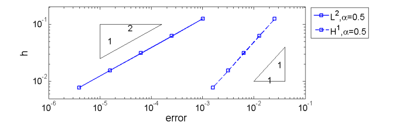
Figure 1. Numerical results, i.e., errors $\|u(t)-{\bar{u}}_{h}(t)\|_{\dot{H}^{p}(\Omega)}$, $p=0,1$ at $t=1$, for example (1a) (nonsmooth data) with $\alpha=0.5$.

5.1.2. Numerical results for example (1b)

In this example, we consider the case of very weak data, which involves the Dirac $\delta$-function. Since the Dirac $\delta$-function $\delta_{1/2}(x)$ is a bounded linear functional on $C_{0}(0,1)$. and $H_{0}^{1/2+\epsilon}(0,1)$ with $\epsilon>0$ embeds continuously into $C_{0}(0,1)$, we have $\delta_{1/2}(x)\in H^{-1/2-\epsilon}(\Omega)$. Thus, the source term $f(x,t)=(\chi_{[1/2,1]}(t)+1)\delta_{1/2}(x)\in L^{\infty}(0,T;H^{-1/2-\epsilon}(\Omega))$. In Table 3 we show the error and convergence rates for the lumped mass method for three different $\alpha$ values. Here the mesh size is chosen to be $h=1/(2^{k}+1)$, and thus the Dirac $\delta$ function is not aligned with the grid. The results indicate an $O(h^{1/2})$ and $O(h^{3/2})$ convergence rate for the $H^{1}(\Omega)$- and $L^{2}(\Omega)$-norm of the error, respectively, which agrees well with the theoretical prediction. In Table 4, we report the results for the case that the $\delta$-function is supported at a grid point. We observe that the method converges at the expected rate in $H^{1}(\Omega)$-norm, while the convergence rate in the $L^{2}(\Omega)$-norm is $O(h^{2})$, i.e., the method exhibits a superconvergence of one half order, which theoretically remains to be established. The plots of the results for $\alpha=0.5$ in Tables 3 and 4 are shown respectively in Figures 2 and 3 in a log-log scale.

Table 3. Numerical results, i.e., errors $\|u(t)-{\bar{u}}_{h}(t)\|_{\dot{H}^{p}(\Omega)}$, $p=0,1$ at $t=1$, for example (1b) (Dirac $\delta$-function) with mesh sizes $h=1/(2^{k}+1)$.

$\alpha$	$k$	$3$	$4$	$5$	$6$	$7$	rate
$\alpha=0.1$	$L^{2}$-norm	5.35e-3	2.07e-3	7.67e-4	2.78e-4	9.94e-5	$O(h^{1.44})$
	$H^{1}$-norm	1.56e-1	1.14e-1	8.23e-2	5.88e-2	4.17e-2	$O(h^{0.48})$
$\alpha=0.5$	$L^{2}$-norm	5.38e-3	2.08e-3	7.68e-4	2.78e-4	9.95e-5	$O(h^{1.44})$
	$H^{1}$-norm	1.57e-1	1.15e-1	8.25e-2	5.89e-2	4.17e-2	$O(h^{0.48})$
$\alpha=0.95$	$L^{2}$-norm	5.39e-3	2.08e-3	7.69e-4	2.79e-4	9.95e-5	$O(h^{1.44})$
	$H^{1}$-norm	1.58e-1	1.15e-1	8.26e-2	5.89e-2	4.18e-2	$O(h^{0.48})$

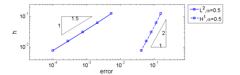
Figure 2. Numerical results, i.e., errors $\|u(t)-{\bar{u}}_{h}(t)\|_{\dot{H}^{p}(\Omega)}$, $p=0,1$ at $t=1$, for example (1b) (Dirac $\delta$-function) with $\alpha=0.5$. The Dirac $\delta$-function is not aligned with grid points.

Table 4. Numerical results, errors $\|u(t)-{\bar{u}}_{h}(t)\|_{\dot{H}^{p}(\Omega)}$, $p=0,1$ at $t=1$, for example (1b) (Dirac $\delta$ function) with mesh sizes $h=1/2^{k}$.

$\alpha$	$k$	$3$	$4$	$5$	$6$	$7$	rate
$\alpha=0.1$	$L^{2}$-norm	1.59e-4	3.93e-5	9.80e-6	2.45e-6	6.15e-7	$O(h^{2.00})$
	$H^{1}$-norm	5.46e-2	3.91e-2	2.78e-2	1.97e-3	1.39e-3	$O(h^{0.49})$
$\alpha=0.5$	$L^{2}$-norm	7.12e-5	1.76e-5	4.37e-6	1.10e-6	2.76e-7	$O(h^{2.00})$
	$H^{1}$-norm	5.53e-2	3.93e-2	2.79e-2	1.97e-3	1.40e-3	$O(h^{0.50})$
$\alpha=0.95$	$L^{2}$-norm	4.91e-5	1.21e-5	3.03e-6	7.66e-7	1.96e-7	$O(h^{2.02})$
	$H^{1}$-norm	5.60e-2	3.96e-2	2.80e-2	1.98e-3	1.40e-3	$O(h^{0.50})$

Figure 3. Numerical results, i.e., errors $\|u(t)-{\bar{u}}_{h}(t)\|_{\dot{H}^{p}(\Omega)}$, $p=0,1$, $t=1$, for example (1b) (Dirac $\delta$-function) with $\alpha=0.5$. The Dirac $\delta$-function is aligned with grid points.

5.1.3. Numerical results for example (1c)

Here the coefficient is variable, and the discrete solution ${\bar{u}}_{h}$ does not have a convenient explicit representation. Hence, we apply the fully discrete scheme with finite difference discretization on time by (5.1). The benchmark solution $u$ is computed on a very fine mesh, i.e., with a spacial mesh size $h=1/512$ and a time step size $\tau=1.0\times 10^{-5}$. The $L^{2}(\Omega)$- and $H^{1}(\Omega)$-norms of the error are reported in Table 5 at $t=1$ for $\alpha=0.5$. The results confirm the discussions in Section 3.5.

Table 5. Numerical results, i.e., errors $\|u(t)-{\bar{u}}_{h}(t)\|_{\dot{H}^{p}(\Omega)}$, $p=0,1$, at $t=1$, for example (1c) (variable coefficients) with $\alpha=0.5$ and mesh sizes $1/2^{k}$.

$h$	$1/8$	$1/16$	$1/32$	$1/64$	$1/128$	rate
$L^{2}$-error	8.42e-4	2.14e-4	5.38e-5	1.34e-5	3.30e-6	$O(h^{2.00})$
$H^{1}$-error	1.76e-2	8.89e-3	4.45e-3	2.21e-3	1.08e-3	$O(h^{1.01})$

5.2. 2-d Examples

Now we consider (1) for $d=2$ on the unit square $\Omega=[0,1]^{2}$ for the following data:

1. Nonsmooth data: $f(x,t)=(\chi_{[1/2,1]}(t)+1)\chi_{[1/4,3/4]\times[1/4,3/4]}$.

2. Very weak data: $f(x,t)=(\chi_{[1/2,1]}(t)+1)\delta_{\Gamma}$ with $\Gamma$ being the boundary of the square $[1/4,3/4]\times[1/4,3/4]$ with $\langle\delta_{\Gamma},\phi\rangle=\int_{\Gamma}\phi(s)ds$. One may view $(v,\chi)$ for $\chi\in X_{h}\subset\dot{H}^{1/2+\epsilon}(\Omega)$ as duality pairing between the spaces $H^{-1/2-\epsilon}(\Omega)$ and $\dot{H}^{1/2+\epsilon}(\Omega)$ for any $\epsilon>0$ so that $\delta_{\Gamma}\in H^{-1/2-\epsilon}(\Omega)$. Indeed, it follows from Hölder’s inequality and the continuity of the trace operator from $\dot{H}^{{1/2}+\epsilon}(\Omega)$ to $L^{2}(\Gamma)$ [2] that

   $$\|\delta_{\Gamma}\|_{H^{-1/2-\epsilon}(\Omega)} =\sup_{\phi\in\dot{H}^{1/2+\epsilon}(\Omega)}\frac{|\int_{\Gamma}\phi(s)ds|}{\|\phi\|_{\dot{H}^{1/2+\epsilon}(\Omega)}}\leq|\Gamma|^{1/2}\sup_{\phi\in\dot{H}^{1/2+\epsilon}(\Omega)}\frac{\|\phi\|_{L^{2}(\Gamma)}}{\|\phi\|_{\dot{H}^{1/2+\epsilon}(\Omega)}}\leq C.$$

To discretize the problem, we divide $(0,1)$ into $N=2^{k}$ equally spaced subintervals with a mesh size $h=1/N$ so that unit square $(0,1)^{2}$ is divided into $N^{2}$ small squares. We get a symmetric triangulation of the domain $(0,1)^{2}$ by connecting the diagonal of each small square. Therefore, the lumped mass method and standard Galerkin method have the same convergence rates. On these meshes, $\bar{\lambda}^{h}_{n,m}$ and $\bar{\varphi}^{h}_{n,m}$, $1\leq n,m\leq N-1$, i.e., eigenvalues and eigenvectors of the discrete Laplacian $\bar{\Delta}_{h}$, are explicitly given by:

$$\bar{\lambda}^{h}_{n,m}=\frac{4}{h^{2}}\left(\sin^{2}\frac{n\pi h}{2}+\sin^{2}\frac{m\pi h}{2}\right),\quad\bar{\varphi}^{h}_{n,m}(x_{i},y_{j})=2\sin(n\pi x_{i})\sin(m\pi y_{j}).$$

respectively, where $(x_{i},y_{j})$, $i,j=1,\ldots,N-1$, is a mesh point. Then the semidiscrete approximation can be computed via the explicit representation (4.6).

5.2.1. Numerical results for example (2a)

In this example the right hand side data $f(x,t)$ is in the space $L^{\infty}(0,1;\dot{H}^{1/2-\epsilon}(\Omega))$ with $\epsilon>0$, and the numerical results were computed at $t=1$ for $\alpha=0.1,0.5$ and $0.95$; see Table 6 and Figure 4. The slopes of the error curves in a log-log scale are $2$ and $1$, respectively, for $L^{2}(\Omega)$- and $H^{1}(\Omega)$-norm of the errors, which agrees well with the theoretical results for the nonsmooth case.

Table 6. Numerical results, i.e., errors $\|u(t)-{\bar{u}}_{h}(t)\|_{\dot{H}^{p}(\Omega)}$, $p=0,1$ at $t=1$, for example (2a) (nonsmooth data) with mesh sizes $h=1/2^{k}$ in either direction.

$\alpha$	$k$	$3$	$4$	$5$	$6$	$7$	rate
$\alpha=0.1$	$L^{2}$-norm	9.66e-4	2.48-4	6.26e-5	1.57e-5	3.93e-6	$O(h^{1.99})$
	$H^{1}$-norm	2.06e-2	1.04e-2	5.24e-3	2.63e-3	1.31e-3	$O(h^{0.99})$
$\alpha=0.5$	$L^{2}$-norm	9.82e-4	2.52-4	6.36e-5	1.59e-5	3.99e-6	$O(h^{1.99})$
	$H^{1}$-norm	2.10e-2	1.07e-2	5.35e-3	2.68e-3	1.34e-3	$O(h^{0.99})$
$\alpha=0.95$	$L^{2}$-norm	9.82e-4	2.52-4	6.36e-5	1.61e-5	4.02e-6	$O(h^{1.99})$
	$H^{1}$-norm	2.13e-2	1.08e-2	5.42e-3	2.71e-3	1.36e-3	$O(h^{0.99})$

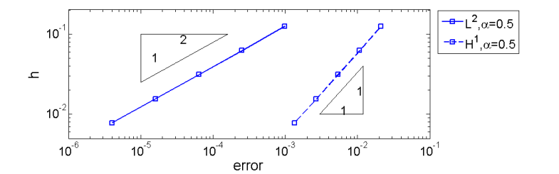
Figure 4. Numerical results, i.e., errors $\|u(t)-{\bar{u}}_{h}(t)\|_{\dot{H}^{p}(\Omega)}$, $p=0,1$, at $t=1$, for example (2a) (nonsmooth data) with $\alpha=0.5$.

5.2.2. Numerical results for example (2b)

In Table 7, we present the $L^{2}(\Omega)$- and $H^{1}(\Omega)$-norms of the error for this example. The $H^{1}(\Omega)$-norm of the error decays at the theoretical rate, however the $L^{2}(\Omega)$-norm of the error exhibits superconvergence. This is attributed to the fact that the boundary $\Gamma$ is fully aligned with element edges. In contrast, if we choose $P_{h}f$ as the discrete right hand side for the lumped mass semidiscrete problem instead of $\bar{P}_{h}f$, then the $L^{2}(\Omega)$-norm of the error converges only at the standard order; see Table 8.

Table 7. Numerical results, i.e., errors $\|u(t)-{\bar{u}}_{h}(t)\|_{\dot{H}^{p}(\Omega)}$, $p=0,1$ at $t=1$, for example (2b) (Dirac $\delta$-function) with mesh sizes $h=1/2^{k}$ in either direction.

$\alpha$	$k$	$3$	$4$	$5$	$6$	$7$	rate
$\alpha=0.1$	$L^{2}$-norm	4.61e-3	1.25e-3	3.31e-4	8.68e-5	2.39e-5	$O(h^{1.90})$
	$H^{1}$-norm	1.60e-1	9.92e-2	6.43e-2	4.43e-2	3.16e-2	$O(h^{0.58})$
$\alpha=0.5$	$L^{2}$-norm	4.67e-3	1.26e-3	3.34e-4	8.76e-5	2.40e-5	$O(h^{1.91})$
	$H^{1}$-norm	1.60e-1	9.92e-2	6.44e-2	4.50e-2	3.17e-2	$O(h^{0.58})$
$\alpha=0.95$	$L^{2}$-norm	4.70e-3	1.27e-3	3.36e-4	8.81e-5	2.42e-5	$O(h^{1.91})$
	$H^{1}$-norm	1.61e-1	9.98e-2	6.46e-2	4.50e-2	3.17e-2	$O(h^{0.58})$

Table 8. Numerical results, i.e., errors $\|u(t)-{\bar{u}}_{h}(t)\|_{\dot{H}^{p}(\Omega)}$, $p=0,1$, at $t=1$, for example (2b) (Dirac $\delta$-function) with $f_{h}=P_{h}f$ and mesh sizes $h=1/2^{k}$ in either direction.

$\alpha$	$k$	$3$	$4$	$5$	$6$	$7$	rate
$\alpha=0.5$	$L^{2}$-norm	1.19e-2	4.55e-3	1.69e-3	6.15e-4	2.22e-4	$O(h^{1.44})$
	$H^{1}$-norm	3.28e-1	2.32e-1	1.67e-1	1.13e-1	8.21e-2	$O(h^{0.50})$

6. conclusion

In this paper, we have studied two semidiscrete finite element schemes, i.e., the semidiscrete Galerkin method and the lumped mass method, for the time-fractional diffusion problem with a nonsmooth right hand side $f\in L^{\infty}(0,T;\dot{H}^{q}(\Omega))$, with $-1<q\leq 1$. We derived almost optimal estimates of the error and its gradient for the Galerkin method, and also almost optimal estimates of the gradient of the error for the lumped mass method. Optimal estimates for the $L^{2}(\Omega)$-norm of the error can only be shown under certain restrictions on the mesh such that condition (4.11) is fulfilled. There are several possible extensions of the work. First, the error estimates are expected to be useful for analyzing relevant inverse problems, which will be studied in a future work. Second, it is natural to study the fully discrete scheme, e.g., with finite difference or discontinuous Galerkin method in time.

References

- [1] E. E. Adams and L. W. Gelhar. Field study of dispersion in a heterogeneous aquifer: 2. spatial moments analysis. Water Res. Research, 28(12):3293 –3307, 1992.
- [2] R. A. Adams and J. J. F. Fournier. Sobolev Spaces. Elsevier/Academic Press, Amsterdam, second edition, 2003.
- [3] B. Berkowitz, J. Klafter, R. Metzler, and H. Scher. Physical pictures of transport in heterogeneous media: Advection-dispersion, random-walk, and fractional derivative formulations. Water Res. Research, 38(10):9–1–9–12, 2002.
- [4] P. Chatzipantelidis, R. Lazarov, and V. Thomée. Some error estimates for the lumped mass finite element method for a parabolic problem. Math. Comp., 81(277):1–20, 2012.
- [5] J. Cheng, J. Nakagawa, M. Yamamoto, and T. Yamazaki. Uniqueness in an inverse problem for a one-dimensional fractional diffusion equation. Inverse Problems, 25(11):115002, 1–16, 2009.
- [6] M. Giona, S. Cerbelli, and H. E. Roman. Fractional diffusion equation and relaxation in complex viscoelastic materials. Phys. A, 191(1–4):449–453, 1992.
- [7] Y. Hatano and N. Hatano. Dispersive transport of ions in column experiments: An explanation of long-tailed profiles. Water Res. Research, 34(5):1027–1033, 1998.
- [8] B. Jin, R. Lazarov, J. Pasciak, and Z. Zhou. Galerkin fem for fractional order parabolic equations with initial data in . Proc. 5th Conf. Numer. Anal. Appl. (June 15-20, 2012), Springer, in press, 2013.
- [9] B. Jin, R. Lazarov, and Z. Zhou. Error estimates for a semidiscrete finite element method for fractional order parabolic equations. SIAM J. Numer. Anal., 51(1):445–466, 2013.
- [10] B. Jin and W. Rundell. An inverse problem for a one-dimensional time-fractional diffusion equation. Inverse Problems, 28(7):075010, 19 pp., 2012.
- [11] Y. L. Keung and J. Zou. Numerical identifications of parameters in parabolic systems. Inverse Problems, 14(1):83–100, 1998.
- [12] A. Kilbas, H. Srivastava, and J. Trujillo. Theory and Applications of Fractional Differential Equations. Elsevier, Amsterdam, 2006.
- [13] X. Li and C. Xu. A space-time spectral method for the time fractional diffusion equation. SIAM J. Numer. Anal., 47(3):2108–2131, 2009.
- [14] Y. Lin and C. Xu. Finite difference/spectral approximations for the time-fractional diffusion equation. J. Comput. Phys., 225(2):1533–1552, 2007.
- [15] W. McLean and V. Thomée. Maximum-norm error analysis of a numerical solution via Laplace transformation and quadrature of a fractional-order evolution equation. IMA J. Numer. Anal., 30(1):208–230, 2010.
- [16] W. McLean and V. Thomée. Numerical solution via Laplace transforms of a fractional order evolution equation. J. Int. Eq. Appl., 22(1):57–94, 2010.
- [17] E. W. Montroll and G. H. Weiss. Random walks on lattices. II. J. Math. Phys., 6(2):167–181, 1965.
- [18] K. Mustapha. An implicit finite-difference time-stepping method for a sub-diffusion equation, with spatial discretization by finite elements. IMA J. Numer. Anal., 31(2):719–739, 2011.
- [19] R. Nigmatulin. The realization of the generalized transfer equation in a medium with fractal geometry. Phys. Stat. Sol. B, 133:425–430, 1986.
- [20] I. Podlubny. Fractional Differential Equations. Academic Press, San Diego, CA, 1999.
- [21] K. Sakamoto and M. Yamamoto. Initial value/boundary value problems for fractional diffusion-wave equations and applications to some inverse problems. J. Math. Anal. Appl., 382(1):426–447, 2011.
- [22] H. Seybold and R. Hilfer. Numerical algorithm for calculating the generalized Mittag-Leffler function. SIAM J. Numer. Anal., 47(1):69–88, 2008/09.
- [23] V. Thomée. Galerkin Finite Element Methods for Parabolic Problems, volume 25 of Springer Series in Computational Mathematics. Springer-Verlag, Berlin, 1997.
- [24] J. Xie and J. Zou. Numerical reconstruction of heat fluxes. SIAM J. Numer. Anal., 43(4):1504–1535, 2006.
- [25] S. Yuste and L. Acedo. An explicit finite difference method and a new von Neumann-type stability analysis for fractional diffusion equations. SIAM J. Numer. Anal., 42(5):1862–1874, 2005.