Exotic matter influence on the polar quasi-normal modes of neutron stars with equations of state satisfying the $2M_{\odot}$ constraint.

Abstract

In this paper we analyze the quasi-normal mode spectrum of realistic neutron stars by studying the polar modes. In particular we study the spatial wI mode, the f mode, and the fundamental p mode. The study has been done for 15 different equations of state containing exotic matter and satisfying the $2M_{\odot}$ constraint. Since f and p modes couple to matter perturbations, the influence of the presence of hyperons and quarks in the core of the neutron stars is more significant than for the axial component. We present phenomenological relations for the frequency and damping time with the compactness of the neutron star. We also consider new phenomenological relations between the frequency and damping time of the w mode and the f mode. These new relations are independent of the equation of state, and could be used to estimate the central pressure, mass or radius, and eventually constrain the equation of state of neutron stars. To obtain these results we have developed a new method based on the Exterior Complex Scaling technique with variable angle.

I Introduction

Neutron stars can be used as probes to gain insight into the structure of matter at high densities ($10^{15}g/cm^{3}$ at their core). Knowledge on mass, radius, and any other global property of the neutron star can give us important information on the state and composition of matter at those extreme physical conditions. But, although the mass can be determined with quite good precision, a direct measurement of the radius is currently very difficult using astrophysical observations.

Nevertheless, the detection of gravitational waves originated in the neutron stars could be used to obtain estimations, or at least constrains, on the value of the gravitational radius of the star. With knowledge on the mass and radius, we would be able to have a better understanding of the behavior of matter at high density and pressure. So the study of these gravitational waves are crucial in the understanding of the physics of matter at extreme densities.

Neutron stars present a layer structure which can be essentially described by two very different regions: a core (where exotic matter could be found) enveloped by a crust (with a solid crystalline structure similar to a metal). The relativistic fluid that compose the neutron star can be described as a perfect fluid, for which the equation of state is needed. Because not so much information is available beyond the nuclear densities, the EOS is very model dependent, since different particle populations may appear at those energies Haensel and Yakovlev (2007); Glendenning (2000). Another interesting feature is that along the core of the star and specially in the core-crust interface, first order phase transitions could be found in realistic equations of state. These phase transitions result in small discontinuities in the energy density of the star matter Haensel and Yakovlev (2007); Heiselberg and Hjorth-Jensen (2000).

Very interesting information can be obtained from the recent measurement of the mass of PSR J1614-2230, of $1.97M_{\odot}$, which impose constraints on equations of state for exotic matter that could be found on neutron stars Prakash and Lattimer (2011). Several equations of state that are able to produce neutron star configurations with $2M_{\odot}$ and exotic matter in their cores have been proposed Bednarek, I. et al. (2012); Bonanno, Luca and Sedrakian, Armen (2012); Weissenborn et al. (2012, 2011). If other global parameters could be measured, more important constraints could be imposed to the equation of state.

If an internal or external event perturbate a neutron star, it may oscillate non radially, emitting gravitational waves to the space Sathyaprakash and Schutz (2009). Large-scale interferometric gravitational wave detectors LIGO, GEO, TAMA and VIRGO, have reached the original design sensitivity, and the detection of the first gravitational waves could happen in the next years Pitkin et al. (2011). These detections will provide useful information about the composition of the astrophysical objects that generate them, like neutron stars Sathyaprakash and Schutz (2009).

The gravitational waves emitted by a neutron star present dominant frequencies which can be studied using the quasi-normal mode formalism Kokkotas and Schmidt (1999); Nollert (1999); Rezzolla (2003). These eigen-frequencies are given by a complex number. The real part gives us the oscillation frequency of the mode, while the imaginary part gives us the inverse of the damping time. The quasi-normal mode spectrum is quite dependent on the properties of the star, i.e. the equation of state.

Hence, the detection of gravitational radiation from neutron stars combined with a complete theoretical study of the possible spectrums that can be obtained with different equations of state can be very useful in the determination of the matter behavior beyond nuclear matter Benhar et al. (1999a); Kokkotas et al. (2001); Benhar et al. (2004); Benhar (2005); Ferrari and Gualtieri (2008); Chatterjee and Bandyopadhyay (2009); Wen et al. (2009).

The formalism necessary to study quasi-normal modes were first developed for black holes by Regge and Wheeler Regge and Wheeler (1957) and by Zerilli Zerilli (1970). Quasi-normal modes can be differentiated into polar and axial modes. The equation describing the quasi-normal mode perturbation of the Schwarzschild metric is essentially a Schrodinger like equation: the Regge-Wheeler equation for axial perturbations and the Zerilli equation for polar ones. For black holes, both types of modes are space-time modes. The formalism was studied in the context of neutron stars first by Thorne Thorne and Campolattaro (1967); Price and Thorne (1969); Thorne (1969a, b); Campolattaro and Thorne (1970), Lindblom Lindblom and Detweiler (1983); Detweiler and Lindblom (1985), and then reformulated by Chandrasekhar and Ferrari Chandrasekhar and Ferrari (1991a); Chandrasekhar et al. (1991); Chandrasekhar and Ferrari (1991b), Ipser and Price Ipser and Price (1991), and Kojima Kojima (1992). In neutron stars, axial modes are purely space-time modes of oscillation (w-modes), while polar modes can be coupled to fluid oscillations (fundamental f-modes, pressure p-modes, and also a branch of spatial w-modes). In this paper we will consider only polar modes of oscillation. The corresponding study of axial modes can be in found Blázquez-Salcedo et al. (2013).

Although the perturbation equations for neutron stars can be simplified into a Regge-Wheeler equation or a Zerilli equation for the vacuum part of the problem, it is complicated to obtain the quasi-normal modes spectrum of neutron stars. The equations must be solved numerically and no analytical solution is known for physically acceptable configurations. The main difficulty is found on the diverging and oscillatory nature of the quasi-normal modes. These functions are not well handled numerically.

Several methods have been developed to deal with these and other difficulties. For a complete review on the methods see the review by Kokkotas and Schmidt Kokkotas and Schmidt (1999).

The axial part of the spectrum has been extensively studied for simplified constant density models and polytropes (Kokkotas and Schutz (1992); Andersson et al. (1995); Kokkotas (1994)). Important results for the polar spectrum have been obtained using several methods, for example the continued fraction method, which have been used to study realistic equations of state Benhar et al. (1999a, 2004); Wen et al. (2009). More recently, Samuelsson et al Samuelsson et al. (2007) used a complex-radius approach for a constant density configuration to study axial quasi-normal modes.

In order to use the results for future observations, Andersson and Kokkotas, first for polytropes Andersson and Kokkotas (1996) and later for some realistic equations of state Andersson and Kokkotas (1998), proposed some empirical relations between the modes and the mass and the radius of the neutron star that could be used together with observations to constrain the equation of state. In later works Benhar, Ferrari and Gualtieri Benhar et al. (2004, 2007); Ferrari and Gualtieri (2008) reexamined those relations for other realistic equations of state. Recently the authors studied these relations for axial modes, using new equations of state satisfying the 2 $M_{\odot}$ condition Blázquez-Salcedo et al. (2013).

In this work we study similar relations for the polar modes that could be used to estimate global parameters of the star, constraining the equation of state of the core of the neutron star. We present a new approach to calculate quasi-normal modes of realistic neutron stars. Essentially it is the implementation of the method used previously for axial modes in Blázquez-Salcedo et al. (2013) to polar modes. We make use of several well-known techniques, like the use of the phase for the exterior solution and the use of a complexified coordinate to deal with the divergence of the outgoing wave. We also introduce some new techniques not used before in this context: freedom in the angle of the exterior complex path of integration, use of Colsys package to integrate all the system of equations at once with proper boundary and junction conditions and possibility of implementation of phase transition discontinuities. These new techniques allow us to enhance precision, to obtain more modes in shorter times, and also to study several realistic equations of state, comparing results for different compositions.

In Section II we present a brief review on the quasi-normal mode formalism in order to fix notation. In section III we present the numerical method, which has been implemented in Fortran based double-precision programs. In Section IV we present the numerical results used from the application of the method to the study of realistic equations of state. We finish in Section V by presenting a summary of the main points of the paper.

II Overview of the Formalism

In this section we will give a brief review of the formalism used to describe polar quasi-normal modes and the method used to calculate them. We will use geometrized units $(c=1,G=1)$.

We consider polar perturbations on the static spherical space-time describing the star: $ds^{2}=e^{2\nu}dt^{2}-e^{2\lambda}dr^{2}-r^{2}(d\theta^{2}+\sin^{2}\theta d\varphi^{2})$. The matter is considered as a perfect fluid with barotropic equation of state. As it can be demonstrated, only polar modes do couple to the matter perturbations of the star Thorne and Campolattaro (1967)-Kojima (1992), i.e., first order perturbations of the energy density and pressure. Axial modes, which were studied in Blázquez-Salcedo et al. (2013), are only coupled to the Lagrangian displacement of the matter. So the spectrum of polar modes is much more dependent of the matter content of the star than the axial modes.

Up to first order in perturbation theory, and once the gauge is fixed (Regge-Wheeler gauge Nollert (1999)) , the number of functions needed to describe the polar perturbations is eight, which are, following Lindblom notation Lindblom and Detweiler (1983); Detweiler and Lindblom (1985): $(H^{0}_{lm},H^{1}_{lm},H^{2}_{lm},K_{lm},W_{lm},X_{lm},\Pi_{lm},E_{lm})$. Once the Einstein equation is solved, together with the conservation of energy and barion number, we obtain four first order differential equations for $(H^{1}_{lm},K_{lm},W_{lm},X_{lm})$. There is also four algebraic relations for $(H^{0}_{lm},H^{2}_{lm},\Pi_{lm},E_{lm})$.

The angular dependence of the functions is known from the tensor expansion and we will only consider in this work the $l=2$ case. We can extract the time dependence from the functions by making a Laplace transformation resulting in equations explicitly dependent on the eigen-value $\omega$.

Inside of the star we will need to solve the well known zero order system of equations for hydrostatic equilibrium of an spherical star. We need to specify the equation of state for the matter. Once we have an static solution we can solve the system of four differential equations for the perturbations.

Outside the star (no matter), it can be seen that the system of equations can be rewritten and it is reduced to a single second order differential equation (Zerilli equation):

$$\frac{d^{2}Z_{lm}}{dy^{2}}+\left[\omega^{2}-V(r)\right]Z_{lm}=0,$$ (1)

where $y$ is the tortoise coordinate,

$$y=\int_{0}^{r}e^{\lambda-\nu}dr,$$ (2)

and the eigen-frequency of the polar mode is a complex number $\omega=\omega_{\Re}+i\omega_{\Im}$. The potential can be written as:

$$V(r)=2(r-2M)\tfrac{n^{2}(n+1)r^{3}+3Mn^{2}r^{2}+9M^{2}nr+9M^{3}}{r^{4}(nr+3M)^{2}},$$ (3)

where $n=(l+2)(l-1)/2$ and $l=2$ in this work.

III Numerical Method

Note that in general the perturbation functions are complex functions. So numerically we will have to integrate eight real first order differential equations for the perturbation functions inside the star. These also translates into a set of two real second order differential equations outside the star.

The perturbation has to satisfy a set of boundary conditions that can be obtained from the following two requirements Chandrasekhar and Ferrari (1991a): i) the perturbation must be regular at the center of the star, and ii) the resulting quasi-normal mode must be a pure outgoing wave.

In general a quasi-normal mode will be a composition of incoming and outgoing waves, i.e.

$$\lim_{r_{*}\to\infty}Z^{in}\sim e^{i\omega r_{*}},\lim_{r_{*}\to\infty}Z^{out}\sim e^{-i\omega r_{*}}.$$ (4)

Note that, while the real part of $\omega$ determines the oscillation frequency of the wave, the imaginary part of the eigen-value determines the asymptotic behavior of the quasi-normal mode. Outgoing quasi-normal modes are divergent at radial infinity, while ingoing ones tends exponentially to zero as the radius grows. We should impose the solution to behave as a purely outgoing quasi-normal mode at a very distant point. This has the inconvenience that any small contamination of the outgoing signal gives rise to an important incoming wave component.

We have adapted a method based on Exterior Complex Scaling method, that we will describe briefly in the following paragraphs. It is an adaptation to polar modes of the method previously employed for axial quasi-normal modes Blázquez-Salcedo et al. (2013).

Outside the star, and following Andersson (1992)-Samuelsson et al. (2007), we study the phase function (logarithmic derivative of the Z function), which does not oscillate towards asymptotic infinity. Although the phase allows us to eliminate the oscillation, we can not distinguish between the mixed incoming and outgoing waves and the purely outgoing ones. To do so we can study an analytical extension of the phase function, rotating the radial coordinate into the complex plane. This technique of complexification of the integration variable is called Exterior Complex Scaling Aguilar and Combes (1971); Balslev and Combes (1971); Simon (1972).

In our method, the angle of the integration path is treated as a free parameter of the solution. This angle can be adjusted appropriately to enhance precision and reduce integration time.

The use of the phase and Exterior Complex Scaling with variable angle allows us to compactify, so we can impose the outgoing quasi-normal mode behavior as a boundary condition at infinity without using any cutoff for the radial coordinate.

The interior part is integrated satisfying the regularity condition at the origin. We integrate together the zero order and the Zerilli equation. In this way, we can automatically generate more points in the zero order functions if we require a more precise result in our quasi-normal modes.

Because we are interested in realistic equations of state, the implementation of the EOS is a fundamental step of the procedure. We use two possibilities. The first one, a piece-wise polytrope approximation, done by Read et al Read et al. (2009) for 34 different equations of state, where the EOS is approximated by a polytrope in different density-pressure intervals. For densities below the nuclear density, the SLy equation of state is considered. The second kind of implementation for the equation of state, more general, is a piecewise monotone cubic Hermite interpolation satisfying local thermodynamic conditions Fritsch and Carlson (1980).

We implement this method into different Fortran programs and routines, making use of the Colsys package Ascher et al. (1979) to solve numerically the differential equations. The advantage of this package is that it allows the utilization of quite flexible multi-boundary conditions and an adaptative mesh that increases precision

The full solution is generated using two independent solutions of the perturbation equations for the same static configuration and value of $\omega$. The proper matching of a combination of these two interior solutions with the exterior phase will give us an outgoing quasi-normal mode. After a careful study of the matching conditions it can be demonstrated that the junction can be written in terms of a determinant of a $2\times 2$ matrix. The determinant is zero only if the junction conditions are satisfied. That is, a combination of the interior solutions can be matched to the exterior phase, an outgoing wave. The determinant of this matrix, once the static configuration is fixed, only depends on the values $(\omega_{\Re},\omega_{\Im})$. So if for a fixed configuration, a value of the eigen-frequency makes the determinant null, that couple of values $(\omega_{\Re},\omega_{\Im})$ corresponds to a quasi-normal mode of the static configuration. Then, the behavior of the perturbation functions can be analyzed to deduce if the quasi-normal mode is a w-mode, a p-mode or a f-mode.

In figures 1 we show a particular solution for the interior of a neutron star of $1.4M_{\odot}$, equation of state GNH3. They correspond to the f-mode and the fundamental p-mode.

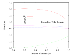
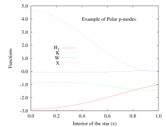
Figure 1: Typical form of the functions integrated inside of the star for f-modes and p-modes.

IV Results

In this section we present our results for the polar quasi-normal modes of neutron stars with realistic equations of state. We consider a wide range of equations of state in order to study the influence of exotic matter on the polar quasi-normal modes. For a similar study performed on the axial component of the spectra see Blázquez-Salcedo et al. (2013).

We start presenting the equations of state used in the study:

Using the parametrization presented by Read et all Read et al. (2009), we have considered SLy, GNH3, H4, ALF2, ALF4.

After the recent measurement of the $1.97M_{\odot}$ for the pulsar PSR J164-2230, several new equations of state have been proposed. These EOS take into account the presence of exotic matter in the core of the neutron star, and they have a maximum mass stable configuration over $1.97M_{\odot}$. We have considered the following ones: two equations of state presented by Weissenborn et al with hyperons in Weissenborn et al. (2012), we call them WCS1 and WCS2; three EOS presented by Weissenborn et al with quark matter in Weissenborn et al. (2011), we call them WSPHS1, WSPHS2, WSPHS3; four equations of state presented by L. Bonanno and A. Sedrakian in Bonanno, Luca and Sedrakian, Armen (2012); we call them BS1, BS2, BS3, BS4; and one EOS presented by Bednarek et al in Bednarek, I. et al. (2012), we call it BHZBM.

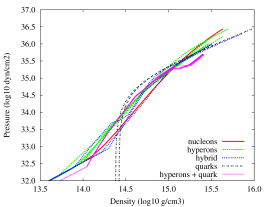
Figure 2: Pressure versus density in logarithmic scale for the 15 equations of state considered, in the high density region.

In Figure 2 we plot all the 15 equations of state we have studied in order to give an idea of the range considered.

We follow the notation previously used in Blázquez-Salcedo et al. (2013). We discuss their characteristics in the following paragraph.

For plain $npe\mu$ nuclear matter we use:

• SLy F. Douchin and P. Haensel (2001) with $npe\mu$ using a potential-method to obtain the EOS.

For mixed hyperon-nuclear matter we use:

• GNH3 Glendenning (1985), a relativistic mean-field theory EOS containing hyperons.

• H4 Lackey et al. (2006), a variant of the GNH3 equation of state.

• WCS1 and WCS2 Weissenborn et al. (2012), two equations of state with hyperon matter, using “model $\sigma\omega\rho\phi$”, and considering ideal mixing, SU(6) quark model, and the symmetric-antisymmetric couplings ratio $\alpha_{v}=1$ and $\alpha_{v}=0.2$ respectively.

• BHZBM Bednarek, I. et al. (2012), a non-linear relativistic mean field model involving baryon octet coupled to meson fields.

For Hybrid stars we use:

• ALF2 and ALF4 Alford et al. (2005), two hybrid EOS with mixed APR nuclear matter and color-flavor-locked quark matter.

• WSPHS3 Weissenborn et al. (2011), a hybrid star calculated using bag model, mixed with NL3 RMF hadronic EOS. The parameters employed are: $B_{eff}^{1/4}=140MeV$, $a_{4}=0.5$, and a Gibbs phase transition.

For Hybrid stars with hyperons and quark color-superconductivity we use:

• BS1, BS2, BS3, and BS4, Bonanno, Luca and Sedrakian, Armen (2012), four equations of state calculated using a combination of phenomenological relativistic hyper-nuclear density functional and an effective NJL model of quantum chromodynamics. The parameters considered are: vector coupling $G_{V}/G_{S}=0.6$ and quark-hadron transition density $\rho_{tr}/\rho_{0}$ equal to $2$, $3$, $3.5$ and $4$ respectively, where $\rho_{0}$ is the density of nuclear saturation.

For quark stars we use:

• WSPHS1 and WSPHS2 Weissenborn et al. (2011). The first equation of state is for unpaired quark matter, and we have considered the parameters $B_{eff}^{1/4}=123.7MeV$,$a_{4}=0.53$. The second equation of state considers quark matter in the CFL phase (paired). The parameters considered are $B_{eff}^{1/4}=130.5MeV$,$a_{4}=0.66$,$\Delta=50MeV$

In Figure 3 we plot the frequencies of all the f-modes, p-modes an wI0-modes obtained for the equations of state considered, in order to present the range in which each modes are found. In the next subsection we will explain the features of each class of modes depending on the equation of state composition: hyperon matter or quark matter.

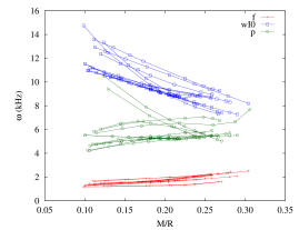
Figure 3: Frequency vs compactness for all the modes studied in this work.

IV.1 Hyperon matter

Fundamental wI mode: At the maximum mass configuration of each EOS (around $2M_{\odot}$), all the equations of state yields frequencies near $8.5Khz$. This is found for stars containing hyperon matter or only nuclear matter. The only exception is the interesting case of the WCS2 (maximum mass of $2.4M_{\odot}$) with the smallest frequency ($7.5Khz$). In general, for one solar mass configurations, the frequency of stars containing hyperon matter is much smaller ($11Khz$) than the frequencies for plain nuclear matter stars ($14Khz$).

In order to use future observations of gravitational waves to estimate the mass and the gravitational radius of the neutron star, as well as to discriminate between different families of equations of state, we obtain empirical relations between the frequency and damping time of quasi-normal modes and the compactness of the star, following Benhar et al. (1999a), Kokkotas et al. (2001), Andersson and Kokkotas (1996) and Andersson and Kokkotas (1998). In Figure 4 we present the frequency of the fundamental mode scaled to the radius of each configuration. The range of the plot is between $1M_{\odot}$ and the maximum mass configuration, so we consider only stable stars. It is interesting to note that even for the softest equations of state with hyperon matter, the scaling relation is very well satisfied. Since the w modes do not couple to matter oscillations, it is not a surprise that this scaled relations are universal.

A linear fit can be made for each equation of state. We fit to the following phenomenological relation:

$$\omega(Khz)=\frac{1}{R(Km)}\left(A\frac{M}{R}+B\right).$$ (5)

In Table 1 we present the fitting parameters $A$,$B$ for each one of the equations of state studied. For all the EOS very similar results are obtained. The empirical parameters are compatible with the empirical relation obtained by Benhar et al Benhar et al. (1999b) for six equations of state.

A similar study can be done to the damping time of the wI0 modes. In Figure 5 we present the damping time of the fundamental mode scaled to the mass of each configuration. In this case, the results can be fitted to a empirical quadratic relation on $M/R$, as follows:

$$\frac{1}{\tau(\mu s)}=\frac{1}{M(M_{\odot})}\left[a\left(\frac{M}{R}\right)^{2}+b\frac{M}{R}+c\right].$$ (6)

In Table 1 we present the fitting parameters a,b and c. Note that they are quite similar for all the equations of state, and also in accordance with the results obtained in Benhar et al. (1999b).

In this relations, as well as in the rest of empirical relations studied in the paper, we have used $G=c=1$, so both mass and radius must be given in units of length (Km), unless otherwise specified.

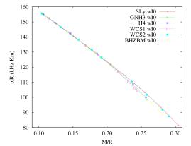
Figure 4: Scaled frequency of the fundamental wI mode vs M/R for hyperon matter EOS. The phenomenological relation is quite independent of the matter composition, as expected from spatial modes

Figure 5: Scaled damping time of the fundamental wI mode vs M/R for hyperon matter EOS.

For a similar study of the axial wI modes using these equations of state see Blázquez-Salcedo et al. (2013).

f mode: Now we will present the results for the f-modes of these configurations. For these modes, the frequency of the SLy stars are always above the hyperon stars considered. The Sly configurations range from $1.6kHz$ for $1M_{\odot}$ to $2.5kHz$ for the maximum mass configuration. Hyperon stars range from $1.3kHz$ for $1M_{\odot}$ to $2.2kHz$, with again the exception of WCS2, that reaches only $2.1kHz$.

In this case one can also study some empirical relations. It is interesting to study the dependence of the frequency with the square root of the mean density. The empirical relations considered for the f modes are the following. For the frequency:

$$\omega(Khz)=U+V\sqrt{\frac{M}{R^{3}}}.$$ (7)

For the damping time:

$$\tau(s)=\frac{R^{4}}{cM^{3}}\left[u+v\frac{M}{R}\right]^{-1}.$$ (8)

In figures 6 and 7 we plot these relations. In Figure 6 it can be seen that (7) is quite different depending on the EOS. Again WCS2 present a very different behavior close to the maximum mass configurations. For the damping time, relation (8) is very well satisfied for every EOS along all the range.

In Table 2 we present the fitting parameters U and V for the frequency, and u and v for the damping time.

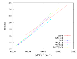
Figure 6: Scaled frequency of the fundamental f mode vs M/R for hyperon matter. Although the frequency is linear with the square root of the mean density, each equation of state has its own particular phenomenological parameters, and so the empirical relation is less useful.

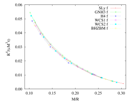
Figure 7: Scaled damping time of the fundamental f mode vs M/R for hyperon matter. In this case, the scaled damping time is quite independent of the equation of state.

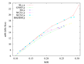
Figure 8: Scaled frequency of the fundamental p mode vs M/R. At high compactness the scaled frequency is more sensible to the presence of hyperon matter, with the exception of WCS2.

Fundamental p mode: The frequency of the fundamental p mode is the most sensitive to the EOS of the configuration. For SLy EOS, the frequency ranges from $5.7kHz$ for $1M_{\odot}$ to $7.8kHz$ for the maximum mass configuration. In the presence of hyperon matter, the range of frequencies is much shorter, variating from $4.6kHz$ for $1M_{\odot}$ to $5.5kHz$ for the maximum mass configuration.

In principle, an interesting empirical relation now could be

$$\omega(Khz)=\frac{1}{M(Km)}\left(K\frac{M}{R}+K_{0}\right).$$ (9)

In figure 8, we present the frequency scaled to the mass, versus the compactness. There is an important resemblance between the Sly EOS and the WCS2, which present a similar behavior for high compact stars. The relation is quite different with respect the rest of hyperon matter EOS. This effect could be used to constraint the value of $\alpha_{v}$ for compact enough stars.

In Table 3 we present the fitting parameters K and K0 for the frequency.

IV.2 Quark matter

Fundamental wI mode: The frequencies for the hybrid EOS ALF4 gives almost the same results as the SLy EOS. The four BS1-4 EOS are essentially similar, with a quite low frequency: $8.8kHz$ for the maximum mass configuration ($2M_{\odot}$). Nevertheless is the WSPHS3 the EOS with lowest frequency: $8kHz$ for the maximum mass configuration ($2.2M_{\odot}$). For pure quark stars WSPHS1-2, even lower frequencies ($7.2kHz$) are obtained at the maximum mass configuration ($2.5M_{\odot}$).

We study the empirical relations (5) and (6) for these equations of state. We present them in figures 9 and 10 for frequency and damping time respectively. It can be seen that the empirical relation is again very well satisfied for all the hybrid equations of state. For the pure quark stars, a similar relation with different parameters is found. The fits can be found in table 4.

Note that, although the empirical relation is also satisfied for pure quark stars, it is slightly different. This is due to the different layer structure of these pure quark stars. These stars are essentially naked quark cores, where the pressure quickly drops to zero in the outer layers, although the density is almost constant.

The study of the axial wI modes using these equations of state can be found in Blázquez-Salcedo et al. (2013).

f mode: The lowest frequency is around $1.2kHz$ for $1M_{\odot}$ stars composed only of quark matter (WSPHS1-2). The higher frequencies are reached at $2.2kHz$ for hybrid stars beyond $2M_{\odot}$. For ALF2-4 frequencies, they approach those of pure nuclear matter. The configurations with EOS WSPH3 and BS1-4 have always lower frequencies than the rest of hybrid stars, but are larger than the pure quark stars. In the case of the damping time there is essentially no difference between the EOS ($0.3s$ for maximum mass configurations), except for WSPHS1-2, which have slightly larger damping times for the most compact ones ($0.4s$ for maximum mass configurations).

We study the dependence of the frequency with square root of the mean density as we did before for hyperon matter. The empirical relations to consider are again (7) and (8). In Figures 11 and 12 we plot these relations. In Figure 11 it can be seen that (7) is quite different depending on the EOS. ALF4 is almost identical to SLy, while the other hybrid equations are in-between these ones and the pure quark EOS. Regarding the damping time (Figure 12), relation (8) is very well satisfied for every hybrid EOS considered along all the range. In table 5 we present the fits to (7) and (8) of these results.

Fundamental p mode: At high compactness, ALF4 has higher frequencies (near $7khz$) than the rest of hybrid EOS (for example BS1-4 and WSPHS1-2 have similar frequencies around $5.2kHz$). The highest frequencies are reached for pure quark stars at $1M_{\odot}$, with $10kHz$.

In Figure 13 we present the empirical relations (9). It can be seen that all hybrid equations lay in the same range although the linear relation is not very well satisfied for higher compactness. In the case of pure quark stars, the situation is much worse. In table 6 we present the fits to (9) for each equation of state.

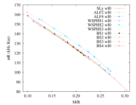
Figure 9: Scaled frequency of the fundamental wI mode vs M/R for EOS containing quarks. Note that the pure quark configurations of EOS WSPHS1-2 present a different set of phenomenological parameters.

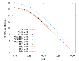
Figure 10: Scaled damping time of the fundamental wI mode vs M/R for EOS containing quarks. Hybrid and quark stars has different parameters in the empirical relations.

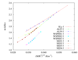
Figure 11: Scaled frequency of the fundamental f mode vs M/R for EOS containing quarks. In this case, the empirical relation is dependent of the equation of state considered, and so is less useful.

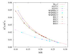
Figure 12: Scaled damping time of the fundamental f mode vs M/R for hybrid and quark stars. The empirical relation is almost insensitive of the EOS, except for the pure quark stars.

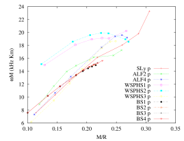
Figure 13: Scaled frequency of the fundamental p mode vs M/R. Once again a general tendency is seen, but the particular phenomenological relation of each EOS is different from the rest. As expected the p mode is very sensitive to the equation of state.

Table 1: Fitting for the wI0 modes. Parameters $A$ and $B$ correspond to the linear empirical relation for the frequency (5). Parameters $a$,$b$ and $c$ correspond to the quadratic empirical relation for the damping time (6).

wI0	SLy	GNH3	H4	WCS1	WCS2	BHZBM
$A$	$-365.3\pm 8.2$	$-371.0\pm 8.6$	$-364.4\pm 1.6$	$-374.4\pm 8.2$	$-365.2\pm 7.2$	$-384.2\pm 8.2$
$B$	$195.3\pm 1.8$	$195.9\pm 1.6$	$194.9\pm 1.6$	$196.7\pm 1.6$	$195.3\pm 1.5$	$198.0\pm 1.8$
$\chi^{2}$	2.523	1.547	1.479	1.06	1.84	2.03
$a$	$-155\pm 31$	$-339\pm 31$	$-330\pm 35$	$-401\pm 16$	$-217\pm 30$	$-253\pm 41$
$b$	$-11\pm 13$	$49\pm 11$	$48\pm 13$	$70\pm 6$	$13\pm 12$	$21\pm 17$
$c$	$19.7\pm 1.3$	$15.1\pm 1.0$	$15.1\pm 1.1$	$13.34\pm 0.51$	$17.6\pm 1.2$	$17.2\pm 1.6$
$\chi^{2}$	$0.10$	$0.041$	$0.0308$	$0.005$	$0.0827$	$0.0968$

Table 2: Fitting for the f modes. Parameters $U$ and $V$ correspond to the linear empirical relation for the frequency (7). Parameters $u$ and $v$ correspond to the linear empirical relation for the damping time (8).

f	SLy	GNH3	H4	WCS1	WCS2	BHZBM
$U$	$0.7041\pm 0.0063$	$0.338\pm 0.018$	$0.337\pm 0.055$	$0.257\pm 0.055$	$0.5330\pm 0.0083$	$0.328\pm 0.026$
$V$	$32.44\pm 0.15$	$43.07\pm 0.55$	$41.5\pm 1.1$	$44.5\pm 1.6$	$34.52\pm 0.24$	$41.93\pm 0.68$
$\chi^{2}$	$1.58\cdot 10^{-5}$	$1.82\cdot 10^{-4}$	$3.75\cdot 10^{-4}$	$7.41\cdot 10^{-4}$	$2.77\cdot 10^{-5}$	$3.14\cdot 10^{-4}$
$u$	$0.065\pm 0.005$	$0.079\pm 0.004$	$0.071\pm 0.006$	$0.070\pm 0.004$	$0.067\pm 0.006$	$0.063\pm 0.005$
$v$	$-0.221\pm 0.023$	$-0.295\pm 0.021$	$-0.255\pm 0.030$	$-0.251\pm 0.022$	$-0.231\pm 0.021$	$-0.213\pm 0.021$
$\chi^{2}$	$1.98\cdot 10^{-5}$	$1.32\cdot 10^{-5}$	$1.72\cdot 10^{-5}$	$7.18\cdot 10^{-6}$	$2.42\cdot 10^{-5}$	$1.33\cdot 10^{-5}$

Table 3: Fitting for the p modes. Parameters $K$ and $K_{0}$ correspond to the linear empirical relation for the frequency (9).

p	SLy	GNH3	H4	WCS1	WCS2	BHZBM
$K$	$74.9\pm 4.5$	$62.2\pm 3.3$	$61.8\pm 3.3$	$59.8\pm 4.8$	$66.8\pm 2.7$	$54.4\pm 4.5$
$K_{0}$	$-0.68\pm 1.0$	$0.368\pm 0.634$	$0.74\pm 0.64$	$1.54\pm 0.90$	$0.616\pm 0.553$	$2.33\pm 0.96$
$\chi^{2}$	$0.65$	$0.218$	$0.249$	$0.401$	$0.260$	$0.590$

Table 4: Fitting for the wI0 modes. Parameters $A$ and $B$ correspond to the linear empirical relation for the frequency (5). Parameters $a$,$b$ and $c$ correspond to the quadratic empirical relation for the damping time (6).

wI0	ALF2	ALF4	WSPHS1	WSPHS2	WSPHS3	BS1	BS2	BS3	BS4
$A$	$-365.3\pm 11.9$	$-368.9\pm 6.7$	$-351.9\pm 12.3$	$-365.5\pm 10.3$	$-342.1\pm 6.7$	$-351.4\pm 4.7$	$-350.0\pm 0.30$	$349.6\pm 2.7$	$353.2\pm 3.2$
$B$	$197.1\pm 2.3$	$193.3\pm 1.4$	$199.0\pm 2.5$	$202.0\pm 2.2$	$191.8\pm 1.3$	$194.2\pm 0.8$	$194.0\pm 0.5$	$193.9\pm 0.5$	$194.4\pm 0.6$
$\chi^{2}$	2.227	1.164	3.326	2.039	0.687	0.251	0.11	0.086	0.149
$a$	$-347\pm 18$	$-281\pm 19$	$-333.9\pm 8.7$	$-332\pm 24$	$-339\pm 21$	$-339\pm 21$	$-473\pm 21$	$-492\pm 29$	$-432\pm 34$
$b$	$56.1\pm 6.9$	$35.9\pm 7.4$	$52.6\pm 3.2$	$53.1\pm 9.6$	$56.3\pm 7.6$	$92.3\pm 6.6$	$99.0\pm 9.2$	$80\pm 11$	$79.9\pm 8.0$
$c$	$14.66\pm 0.63$	$15.93\pm 0.67$	$16.10\pm 0.27$	$16.03\pm 0.92$	$13.97\pm 0.65$	$11.98\pm 0.51$	$11.46\pm 0.71$	$12.79\pm 0.85$	$12.82\pm 0.63$
$\chi^{2}$	$0.0079$	$0.013$	$0.0037$	$0.0204$	$0.0133$	$0.0049$	$0.0096$	$0.0148$	$0.0102$

Table 5: Fitting for the f modes. Parameters $U$ and $V$ correspond to the linear empirical relation for the frequency (7). Parameters $u$ and $v$ correspond to the linear empirical relation for the damping time (8).

f	ALF2	ALF4	WSPHS1	WSPHS2	WSPHS3	BS1	BS2	BS3	BS4
$U$	$0.38\pm 0.06$	$0.79\pm 0.04$	$-0.24\pm 0.07$	$-0.28\pm 0.07$	$0.71\pm 0.06$	$0.37\pm 0.04$	$0.36\pm 0.04$	$0.38\pm 0.04$	$0.36\pm 0.03$
$V$	$38.7\pm 1.6$	$30.0\pm 1.1$	$48.9\pm 2.1$	$49.4\pm 2.1$	$29.2\pm 1.9$	$98.3\pm 1.2$	$38.6\pm 1.3$	$37.9\pm 1.1$	$38.8\pm 1.1$
$\chi^{2}$	$6.03\cdot 10^{-4}$	$4.66\cdot 10^{-4}$	$2.15\cdot 10^{-4}$	$1.67\cdot 10^{-4}$	$5.58\cdot 10^{-4}$	$1.69\cdot 10^{-4}$	$2.04\cdot 10^{-4}$	$1.58\cdot 10^{-4}$	$1.77\cdot 10^{-5}$
$10u$	$0.59\pm 0.04$	$0.70\pm 0.05$	$0.32\pm 0.01$	$0.31\pm 0.02$	$0.79\pm 0.08$	$0.72\pm 0.04$	$0.73\pm 0.04$	$0.73\pm 0.04$	$0.71\pm 0.04$
$v$	$0.21\pm 0.02$	$0.25\pm 0.02$	$0.10\pm 0.01$	$0.09\pm 0.01$	$0.30\pm 0.04$	$0.28\pm 0.03$	$0.29\pm 0.02$	$0.28\pm 0.02$	$0.27\pm 0.02$
$\chi^{2}$	$6.91\cdot 10^{-6}$	$1.45\cdot 10^{-5}$	$7.74\cdot 10^{-7}$	$6.69\cdot 10^{-7}$	$2.48\cdot 10^{-5}$	$7.55\cdot 10^{-6}$	$6.58\cdot 10^{-6}$	$6.84\cdot 10^{-6}$	$7.03\cdot 10^{-6}$

Table 6: Fitting for the p modes. Parameters $K$ and $K_{0}$ correspond to the linear empirical relation for the frequency (9).

p	ALF2	ALF4	WSPHS1	WSPHS2	WSPHS3	BS1	BS2	BS3	BS4
$K$	$54.5\pm 8.9$	$79.9\pm 5.0$	$36.1\pm 5.3$	$22.8\pm 10.1$	$92.1\pm 3.0$	$64.1\pm 2.4$	$65.0\pm 2.2$	$65.1\pm 2.0$	$63.7\pm 2.2$
$K_{0}$	$3.86\pm 1.73$	$-1.0\pm 1.1$	$10.9\pm 1.1$	$13.8\pm 2.2$	$-3.56\pm 0.60$	$1.5\pm 0.4$	$1.38\pm 0.40$	$1.36\pm 0.35$	$1.58\pm 0.41$
$\chi^{2}$	$1.24$	$0.556$	$0.322$	$1.66$	$0.153$	$0.067$	$0.059$	$0.047$	$0.072$

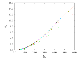
Figure 14: All fundamental wI modes normalized to the square root of the central pressure (equation 10). This scaling make all the wI0 modes lie in the same curve, and could be used to estimate the central pressure as explained in the text.

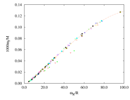
Figure 15: All fundamental f modes scaled as explained in the text. The real part of the eigen-value is scaled to the inverse of the radius. The imaginary part to the inverse of the mass. Since here we choose $c=G=1$, $\omega_{R}/R$ and $\omega_{I}/M$ have units of $cm^{-2}$. This universal relation can be very useful to estimate the radius or mass of a neutron star. Note that all the equations of state, with the exception of the pure quark stars, are found to satisfy the empirical relation 12.

IV.3 Universal Phenomenological Relations

In order to use wave detections coming from neutron stars to estimate global properties like radius or mass, we would like to have empirical relations as much independent from the matter content of the configuration as possible. The empirical relations for the w modes are quite universal, and hence are useful for asteroseismology. On the other hand, the scaled relations for the f mode are still EOS dependent, specially for the frequency. Here we propose some new phenomenological relations that we think could be useful for asteroseismology.

First we present a new empirical relation for the wI fundamental mode. A similar empirical relation for the axial wI modes were first studied in Blázquez-Salcedo et al. (2013).

As it can be seen in figure 14, if the real and the imaginary part are scaled in the following way:

$$\bar{\omega}_{R} = 2\pi\frac{1}{\sqrt{p_{c}(cm^{-2})}}\frac{10^{3}}{c}\omega(Khz),$$

$$\bar{\omega}_{I} = \frac{1}{\sqrt{p_{c}(cm^{-2})}}\frac{10^{6}}{c}\frac{1}{\tau(\mu s)},$$ (10)

that is, normalized in units of the central pressure, taking $c=G=1$, then we obtain the following relation between real and imaginary part of the eigen-value for all the EOS (except WCSHS1-2):

$$\bar{\omega}_{I}=(6.146\pm 0.039)10^{-3}\bar{\omega}_{R}^{2}+$$

$$(-5.57\pm 0.18)10^{-7}\bar{\omega}_{R}^{4},$$ (11)

with $\chi^{2}=0.0214$. The relation is very well satisfied independently of the equation of state, in particular for high density stars. This could be used to approximate the central pressure of the star.

Note that although the empirical relation between $\bar{\omega}_{R}$ and $\bar{\omega}_{I}$ is quite independent of the EOS, the parametrization of the curve in terms of the central pressure is EOS dependent. So if the frequency $\omega(Khz)$ and the damping time $\tau(\mu s)$ are known, we can parametrize a line defining $\bar{\omega}_{R}$ and $\bar{\omega}_{I}$, with parameter $p_{c}$, using the observed frequency and damping time. The observed values will give us the slope of the line. The crossing point of this line with the empirical relation presented in Figure 14 give us an estimation of the central pressure $p_{c}$ independent of the EOS. Now, we can check which EOS is compatible with this $p_{c}$, i.e., which one have the measured wI0 mode near the crossing point for the estimated central pressure. Hence, this method could be used to constrain the equation of state. Note that if mass and radius are already measured, we would have another filter to impose to the EOS.

Concerning the f mode, an analogous relation can be obtained. In this case, by rescaling the real part and the imaginary part in units of the radius and mass respectively. The empirical relation obtained is EOS independent (excluding again WSPHS1-2). It is:

$$(\omega_{I}/M)=(-5.16\pm 0.24)10^{-3}+$$

$$(164.63\pm 0.83)10^{-5}(\omega_{R}/R)+$$

$$(-3.14\pm 0.12)10^{-10}(\omega_{R}/R)^{4},$$ (12)

with $\chi^{2}=1.42\cdot 10^{-6}$. Note that in the formula we have chosen $c=G=1$, so that $\omega_{R}$, $\omega_{I}$, $R$ and $M$ are all given in units of length ($cm$). It is an almost linear relation, although the $(\omega_{R}/R)^{4}$ plays an important role at low compactness configurations. This relation is very well satisfied for every configuration independently of the equation of state, as it can be seen in 15. For pure quark stars the relation is similar but with different parameters, due to the different density-pressure distribution at lower densities. But if only nuclear, hyperon matter and hybrid stars are considered, the empirical relation is universal for these families of equations of state. If the mass of the star emitting the gravitational wave is known by other measurement, this relation could be used to obtain the radius of the star emitting the gravitational wave. Following a procedure similar to the one explained previously for the wI modes, a detection of frequency a damping time of a neutron star emission, whose mass is already known by other measurements, would draw a horizontal line in 15. The intersection of this line with the empirical relation (12) would provide a estimation of the radius of the star.

Combining the two empirical relations (11) and (12), the particular equation of state of the source of the detected emission could be constrained.

V Conclusions

In this paper we have considered the polar quasi-normal modes for realistic neutron stars. In particular, we have obtained results for the fundamental wI mode, the f mode, and the fundamental p mode. The study has been realized for 15 realistic equations of state, all of them satisfying the $2M_{\odot}$ condition, and various compositions: plain nuclear matter, hyperon matter, hybrid and pure quark matter. The numerical procedure developed to obtain the quasi-normal modes is based on Exterior Complex Scaling. A similar study for the axial part of the spectrum can be found in Blázquez-Salcedo et al. (2013).

We have considered empirical relations between the scaled frequencies and damping times of the modes with the compactness and mean density. We have studied in which cases the obtained relations are more independent of the equation of state, and hence, more useful for asteroseismology. We have found that the frequencies of the fundamental p mode and f mode are quite sensitive to the matter composition of the star, so these empirical relations are less useful.

New phenomenological relations have been studied, for the fundamental wI mode and f mode, between the real part and the imaginary part of the fundamental modes. We have found universal empirical relations, independent of the particular equation of state. These relations can be useful in neutron star asteroseismology, allowing to constrain the equation of state, and so providing insight into the state of matter at high densities.