Scalar conservation laws on moving hypersurfaces

Abstract.

We consider conservation laws on moving hypersurfaces. In this work the velocity of the surface is prescribed. But one may think of the velocity to be given by PDEs in the bulk phase. We prove existence and uniqueness for a scalar conservation law on the moving surface. This is done via a parabolic regularization of the hyperbolic PDE. We then prove suitable estimates for the solution of the regularized PDE, that are independent of the regularization parameter. We introduce the concept of an entropy solution for a scalar conservation law on a moving hypersurface. We also present some numerical experiments. As in the Euclidean case we expect discontinuous solutions, in particular shocks. It turns out that in addition to the ”Euclidean shocks” geometrically induced shocks may appear.

1. Introduction

The theoretical and numerical solution of partial differential equations on stationary or moving surfaces has become quite important during the last decade. In many applications PDEs in bulk phases are coupled to PDEs on interfaces between these phases. There is a satisfactory analysis and numerical analysis for elliptic and parabolic equations on stationary or moving surfaces. For references we refer to [11], [12], [14]. Several phenomena like shallow water equations on the earth, relativistic flows, transport processes on surfaces, transport of oil on the waves of the ocean or the transport on moving interfaces between two fluid are modeled by transport equations, and thus hyperbolic PDEs, on fixed or moving surfaces. These equations often are highly nonlinear.

In this work we study scalar conservation laws on moving hypersurfaces without boundary in $\mathbb{R}^{n+1}$. The motion of the surface is prescribed. Assume that $\Gamma(t)$ is a family of smooth and compact hypersurfaces which moves smoothly with time $t\in[0,T]$. When the scalar material quantity $u=u(x,t)$, $x\in\Gamma(t)$, $t\in[0,T]$, is propagated with the surface and simultaneously transported via a given flux $f=f((x,t),u)$ on the surface, then its evolution with respect to prescribed initial values $u_{0}$ is governed by the initial value problem

(1) $$\dot{u}+u\nabla_{\Gamma}\cdot v+\nabla_{\Gamma}\cdot f(\cdot,u)=0\,\,\,\,\,\,\,\mbox{on}\,\,G_{T},\qquad u(\cdot,0)=u_{0}\,\,\mbox{on}\,\,\Gamma_{0}.$$

Here $v$ denotes the velocity of the surface $\Gamma$, and $\nabla_{\Gamma}$ is the surface gradient. The dot stands for a material derivative. $f$ is the given flux function which we assume to be tangentially divergence free on $\Gamma$ and which is a tangent vector to the surface. By $G_{T}$ we denote the space time surface

(2) $$G_{T}=\bigcup_{t\in(0,T)}\Gamma(t)\times\{t\}.$$

The quantities appearing in the PDE (1) are well defined for $u:G_{T}\to\mathbb{R}$ and do not depend on the ambient space.

Let us briefly summarize the published results related to this topic. Total variation estimates for time independent Riemannian manifolds can be found in [20]. The existence proof of entropy solutions on time independent Riemannian manifolds is considered in [7] by viscous approximation. The ideas are based on Kruzkov’s and DiPerna’s theories for the Euclidean case. In a forthcoming paper Lengeler and one of the authors [26] are generalizing the results which we are going to prove in this contribution to the case of time dependent Riemannian manifolds. They show existence and uniqueness (in the space of measure-valued entropy solutions) of entropy solutions for initial values in $L^{\infty}$ and derive total variation estimates if the initial values are in $\operatorname{BV}$. Convergence of finite volume schemes on time independent Riemannian manifolds can be found in [1]. In the paper [25] LeFloch, Okutmustur and Neves prove an error estimate of the form $||u-u_{h}||_{L^{1}}\leq ch^{\frac{1}{4}}$ for the scheme in [1]. The proof generalizes the ideas of the Euclidian case and the convergence rate is the same. This result was generalized to the time dependent case by Giesselmann [16] under the assumption that an entropy solution exists, which we are going to prove in this paper. In [2] an error estimate for hyperbolic conservation laws on an $(N+1)$ dimensional manifold (spacetime), whose flux is a field of differential forms of degree $N$, is shown. The matter Einstein equation for perfect fluids on spacetimes in the context of general relativity is considered in [24]. A wave propagation algorithm for hyperbolic systems on curved manifolds with application in relativistic hydrodynamics and magnetohydrodynamics have been developed and tested in [30], [4], [5], and finite volume scheme on spherical domains, partially with adaptive grid refinement in [8], [5].

This paper is organized as follows. In Section 2 we will summarize the notations and basic relations for moving hypersurfaces which we need to show existence for (1). The PDE in (1) will be derived in Section 3. Since the weak solution of (1) is in general not unique we will define entropy solutions in Section 4. The idea for the existence proof is based on the approximation of the solution of (1) by the solution of a parabolic regularization, which will be presented in Section 5. In Section 6 and 7 we prove uniform estimates in the $H^{1,1}$-norm of the solution of the parabolic regularization. This implies compactness in $L^{1}$ and therefore existence for (1), which is the main subject of Section 8. Since this existence result depends on the special regularization, defined in Section 5, we have to prove uniqueness of (1) in Section 9. With the numerical algorithm described in Section 10 we have performed some numerical experiments. The results are shown in Section 11.

2. Notations and basic relations for moving hypersurfaces

In this Section we present the description of the moving geometry. We use the notion of tangential or surface gradients.

Assumptions 2.1.

Let $\Gamma_{t}=\Gamma(t)\subset\mathbb{R}^{n+1}$ for $t\in[0,T]$ be a time dependent, closed, smooth hypersurface. The initial surface $\Gamma_{0}$ is transported by the smooth function

(3) $$\Phi:\Gamma_{0}\times[0,T]\rightarrow\mathbb{R}^{n+1}$$

with $\Phi(\Gamma_{0},t)=\Gamma_{t}$ and $\Phi(\cdot,0)=Id$. We assume that $\Phi(\cdot,t):\Gamma_{0}\rightarrow\Gamma(t)$ is a diffeomorphism for every $t\in[0,T]$. The velocity of the material points is denoted by $v:=\partial_{t}\Phi\circ\Phi^{-1}$. The tangential flow of a conservative material quantity $u$ with $u(\cdot,t):\Gamma_{t}\rightarrow\mathbb{R}$ is described by a flux function $f=f((x,t),u)$ which is a family of vector fields such that $f((x,t),u)$ is a tangent vector at the surface $\Gamma_{t}$ for $x\in\Gamma_{t}$, $t\in[0,T]$ and $u\in\mathbb{R}$. We assume that all derivatives of f are bounded and that $\nabla_{\Gamma}\cdot f((\cdot,t),s)=0$ for all fixed $t\in\mathbb{R}^{+},s\in\mathbb{R}$. The definition of $\nabla_{\Gamma}\cdot$ is given below.

2.1. Tangential derivatives and geometry

Let us assume that $\Gamma$ is a compact $C^{2}$-hypersurface in $\mathbb{R}^{n+1}$ with normal vector field $\nu$.

Definition 2.2.

For a differentiable function $g:\Gamma\to\mathbb{R}$ we define its tangential gradient as

(4) $$\nabla_{\Gamma}g=\nabla\overline{g}-\nabla\overline{g}\cdot\nu\,\nu,$$

where $\overline{g}$ is an extension of $g$ to a neighbourhood of $\Gamma$. We denote the components of the gradient by

$$\nabla_{\Gamma}g=\left(\underline{D}_{1}g,\dots,\underline{D}_{n+1}g\right).$$

The Laplace-Beltrami operator then is given by

$$\Delta_{\Gamma}g=\nabla_{\Gamma}\cdot\nabla_{\Gamma}g=\sum_{j=1}^{n+1}\underline{D}_{j}\underline{D}_{j}g.$$

It is well known that the tangential gradient only depends on the values of $g$ on $\Gamma$. For more informations about this concept we refer to [10]. With the help of tangential gradients we can describe the geometric properties of $\Gamma$. The matrix

$$\mathcal{H}=\nabla_{\Gamma}\nu,\quad\mathcal{H}_{ij}=\left(\nabla_{\Gamma}\nu\right)_{ij}=\underline{D}_{i}\nu_{j}=\underline{D}_{j}\nu_{i}\quad(i,j=1,\dots,n+1)$$

has a zero eigenvalue in normal direction: $\mathcal{H}\nu=0$. The remaining eigenvalues $\kappa_{1},\dots,\kappa_{n}$ are the principal curvatures of $\Gamma$. We can view the matrix $\mathcal{H}$ as an extended Weingarten map. The mean curvature $H$ of $\Gamma$ is given as the trace of $\mathcal{H}$,

$$H=\sum_{j=1}^{n+1}\mathcal{H}_{jj}=\sum_{j=1}^{n}\kappa_{j},$$

where we note, that this definition of the mean curvature differs from the common definition by a factor $\frac{1}{n}$. Integration by parts on a hypersurface $\Gamma$ is given by the following formula. A proof for surfaces without boundary can be found in [17]. The extension to surfaces with boundary is easily obtained. By $\mu$ we denote the conormal to $\partial\Gamma$.

Lemma 2.3.

(5) $$\int_{\Gamma}\nabla_{\Gamma}g\,=\int_{\Gamma}gH\nu\,+\int_{\partial\Gamma}g\mu\,.$$

Higher order tangential derivatives do not commute. But we have the following law for second derivatives. Here and in the following we use the summation convention that we sum over doubly appearing indices.

Lemma 2.4.

For a function $g\in C^{2}(\Gamma)$ we have for $i,k=1,\dots,n+1$, that

(6) $$\underline{D}_{i}\underline{D}_{k}g=\underline{D}_{k}\underline{D}_{i}g+\mathcal{H}_{kl}\underline{D}_{l}g\nu_{i}-\mathcal{H}_{il}\underline{D}_{l}g\nu_{k}.$$

For the convenience of the reader we give a short proof for this relation.

Proof.

We use the definition (4) of the tangential gradient and extend $g$ constantly in normal direction to obtain $\overline{g}$. Then

$$\underline{D}_{i}\underline{D}_{k}g-\underline{D}_{k}\underline{D}_{i}g=\underline{D}_{i}\left(\overline{g}_{x_{k}}-\overline{g}_{x_{l}}\nu_{l}\nu_{k}\right)-\underline{D}_{k}\left(\overline{g}_{x_{i}}-\overline{g}_{x_{m}}\nu_{m}\nu_{i}\right)$$

$$=\overline{g}_{x_{k}x_{i}}-\overline{g}_{x_{k}x_{r}}\nu_{r}\nu_{i}-\left(\overline{g}_{x_{l}x_{i}}-\overline{g}_{x_{l}x_{s}}\nu_{s}\nu_{i}\right)\nu_{l}\nu_{k}-\overline{g}_{x_{l}}\left(\mathcal{H}_{il}\nu_{k}+\nu_{l}\mathcal{H}_{ik}\right)$$

$$-\overline{g}_{x_{i}x_{k}}+\overline{g}_{x_{i}x_{r}}\nu_{r}\nu_{k}+\left(\overline{g}_{x_{m}x_{k}}-\overline{g}_{x_{m}x_{s}}\nu_{s}\nu_{k}\right)\nu_{m}\nu_{i}+\overline{g}_{x_{m}}\left(\mathcal{H}_{mk}\nu_{i}+\nu_{m}\mathcal{H}_{ik}\right)$$

$$=\overline{g}_{x_{m}}\mathcal{H}_{mk}\nu_{i}-\overline{g}_{x_{l}}\mathcal{H}_{il}\nu_{k}=\mathcal{H}_{kl}\nu_{i}\underline{D}_{l}g-\mathcal{H}_{il}\nu_{k}\underline{D}_{l}g.$$

In the last step we have used that $\mathcal{H}\nu=0$. ∎

2.2. Material derivatives

In this Section we work with moving surfaces.

Definition 2.5.

For a differentiable function $g:G_{T}\to\mathbb{R}$ we define the material derivative

(7) $$\dot{g}=\frac{\partial g}{\partial t}+v\cdot\nabla g.$$

Note that the material derivative only depends on the values of $g$ on the space-time surface $G_{T}$. In our proofs we will frequently use the following formula for the commutation of spatial (tangential) derivatives and (material) time derivatives. A proof is given in the Appendix.

Lemma 2.6.

For $g\in C^{2}(G_{T})$ we have that

(8) $$(\underline{D}_{l}g)\dot{\leavevmode}\nobreak\ =\underline{D}_{l}\dot{g}-A_{lr}(v)\underline{D}_{r}g$$

with the matrix

$$A_{lr}(v)=\underline{D}_{l}v_{r}-\nu_{s}\nu_{l}\underline{D}_{r}v_{s}\quad(l,r=1,\dots,n+1).$$

3. Derivation of the PDE

We derive the conservation law, which we are going to solve in this paper. For this we need the following transport theorem on moving surfaces. A proof can be found in [11].

Lemma 3.1.

(9) $$\frac{d}{dt}\int_{\Gamma}g\,=\int_{\Gamma}\dot{g}+g\nabla_{\Gamma}\cdot v\,.$$

Let $u(\cdot,t)$ be a scalar quantity, defined on $\Gamma(t)$, which is conserved. The conservation law which we are going to solve is given in integral form by

(10) $$\frac{d}{dt}\int_{\gamma(t)}u\,=\int_{\partial\gamma(t)}Q\cdot\mu\,.$$

Here $\gamma(t)$ is a portion of $\Gamma(t)$ which moves in time according to the prescribed velocity $v$. $Q$ is a flux, which we will parametrize later. Obviously normal parts of $Q$ do not enter the conservation law, because the conormal $\mu$ on $\partial\gamma$ is a tangent vector. Thus we may assume that $Q$ is a tangent vector to $\Gamma$. But note, that even if we choose $Q$ as a vector with a normal part, then $Q\cdot\mu=PQ\cdot\mu$ with the projection $P_{ij}=\delta_{ij}-\nu_{i}\nu_{j}$ ($i,j=1,\dots,n+1$).

We apply integration by parts (5) to the right hand side of (10),

$$\int_{\partial\gamma(t)}Q\cdot\mu\,=\int_{\gamma(t)}\nabla_{\Gamma}\cdot Q\,-\int_{\gamma(t)}HQ\cdot\nu\,=\int_{\gamma(t)}\nabla_{\Gamma}\cdot Q\,.$$

To the left hand side of (10) we apply the transport theorem from Lemma 3.1. This leads to

$$\frac{d}{dt}\int_{\gamma(t)}u\,=\int_{\gamma(t)}\dot{u}+u\nabla_{\Gamma}\cdot v\,.$$

Thus the equation (10) is equivalent to

$$\int_{\gamma(t)}\dot{u}+u\nabla_{\Gamma}\cdot v-\nabla_{\Gamma}\cdot Q\,=0,$$

and since $\gamma$ is an arbitrary subregion of $\Gamma$, we arrive at the PDE

$$\dot{u}+u\nabla_{\Gamma}\cdot v-\nabla_{\Gamma}\cdot Q=0.$$

Throughout this paper we assume, that $Q$ has the form

$$Q=-f((x,t),u)\quad(x\in\Gamma(t)),$$

where we assume that

(11) $$f(\cdot,u)\cdot\nu=0\$$

for all $u\in\mathbb{R}$ on $\Gamma$. With this parametrization of the flux the PDE (3) reads

(12) $$\dot{u}+u\nabla_{\Gamma}\cdot v+\nabla_{\Gamma}\cdot(f(\cdot,u))=0\quad\mbox{ on }G_{T}.$$

By the divergence of $f$ we mean the ‘total’ divergence

$$\nabla_{\Gamma}\cdot(f(\cdot,u)) = \sum_{j=1}^{n+1}\underline{D}_{j}f_{j}(\cdot,u)+\sum_{j=1}^{n+1}\frac{\partial f_{j}}{\partial u}(\cdot,u)\underline{D}_{j}u$$

$$= \nabla_{\Gamma}\cdot f(\cdot,u)+f_{u}(\cdot,u)\cdot\nabla_{\Gamma}u.$$

Remark 3.2.

Note, that because of the condition (11) it is in general not possible to choose the flux $f$ independently of $x$ and $t$. If we start with a flux of the form $Q=\tilde{f}(u)$ in the law (10), then the PDE changes to

$$\dot{u}+u\nabla_{\Gamma}\cdot v+\nabla_{\Gamma}\cdot P\tilde{f}(u)=0$$

and we have $f((x,t),u)=P(x,t)\tilde{f}(u)$ in (12).

4. Definition of entropy solutions

As in the Euclidean case classical solutions of (1) do not exist globally in time in general. Therefore we have to introduce the notion of a weak solution.

Definition 4.1.

A function $u\in L^{\infty}(G_{T})$ is called a weak solution of (1) if

(13) $$\int_{0}^{T}\int_{\Gamma}u\dot{\varphi}+f(\cdot,u)\cdot\nabla_{\Gamma}\varphi\,+\int_{\Gamma_{0}}u_{0}\varphi(\cdot,0)\,=0$$

for all test functions $\varphi\in C^{1}(\overline{G_{T}})$ with $\varphi(\cdot,T)=0$.

In general weak solutions are not unique. Therefore we select the entropy solution which will be introduced in Definition 4.3. For the motivation of the entropy condition given in (16), let us consider the following Lemma.

Here and in the following we assume that $u_{0\varepsilon}\in H^{2,1}\cap L^{\infty}$ and

(14) $$\|u_{0\varepsilon}\|_{L^{\infty}(\Gamma_{0})}+\|\nabla_{\Gamma_{0}}u_{0\varepsilon}\|_{L^{1}(\Gamma_{0})}+\varepsilon\|\nabla_{\Gamma_{0}}^{2}u_{0\varepsilon}\|_{L^{1}(\Gamma_{0})}\leq c_{0}$$

with a constant $c_{0}$ which is independent of the parameter $0<\varepsilon\leq 1$.

Lemma 4.2.

Let $f=(f_{1},\dots,f_{n+1})$, $q=(q_{1},\dots,q_{n+1})$, $\eta\in C^{2}(\mathbb{R})$, $\eta^{\prime\prime}\geq 0$. Define $q_{l}(\cdot,s):=\int_{s_{0}}^{s}\eta^{\prime}(\tau)f_{lu}(\cdot,\tau)d\tau$ for $l=1,\dots,n+1$ and let $u_{0}\in L^{\infty}(\Gamma_{0})$. Assume that $u_{\varepsilon}$ is a smooth solution of

(15) $${\dot{u}}_{\varepsilon}+u_{\varepsilon}\nabla_{\Gamma}\cdot v+\nabla_{\Gamma}\cdot f(\cdot,u_{\varepsilon})-\varepsilon\Delta_{\Gamma}u_{\varepsilon}=0\,\,\mbox{on}\,\,G_{T},\quad u_{\varepsilon}(\cdot,0)=u_{0\varepsilon}\,\,\mbox{on}\,\,\Gamma_{0}.$$

If $u_{\varepsilon}\to u$ a.e. on $G_{T}$ and $u_{0\varepsilon}\to u_{0}$ a.e. on $\Gamma_{0}$ for $\varepsilon\to 0$ and $u\in L^{1}(G_{T})$, then $u$ satisfies the entropy condition

(16) $$-\int_{\Gamma_{0}}\eta(u_{0})\phi(\cdot,0)+\int_{0}^{T}\int_{\Gamma_{t}}\big{(}-\eta(u)\dot{\phi}(\cdot,t)-q(\cdot,u)\cdot\nabla_{\Gamma}\phi+\nabla_{\Gamma}\cdot v(u\eta^{\prime}(u)-\eta(u))\phi\big{)}\leq 0$$

for all test functions $\phi\in H^{1}(G_{T})$ with $\phi\geq 0$ and $\phi(\cdot,T)=0$.

Proof.

Let $\eta$ and $q$ be defined as above. We multiply (1) by $\eta^{\prime}(u_{\varepsilon})$ and obtain

(17) $$\dot{u}_{\varepsilon}\eta^{\prime}(u_{\varepsilon})+u_{\varepsilon}\nabla_{\Gamma}\cdot v\eta^{\prime}(u_{\varepsilon})+\nabla_{\Gamma}\cdot f(\cdot,u_{\varepsilon})\eta^{\prime}(u_{\varepsilon})-\varepsilon\Delta_{\Gamma}u_{\varepsilon}\eta^{\prime}(u_{\varepsilon})=0\,\,\,\mbox{on}\,\,G_{T}.$$

This implies

$$\dot{\eta(u_{\varepsilon})}+u_{\varepsilon}\nabla_{\Gamma}\cdot v\eta^{\prime}(u_{\varepsilon})+f_{l}^{\prime}(\cdot,u_{\varepsilon})D_{l}u_{\varepsilon}\eta^{\prime}(u_{\varepsilon})-\varepsilon\Delta_{\Gamma}\eta(u_{\varepsilon})+\varepsilon\eta^{\prime\prime}(u_{\varepsilon})(D_{l}u_{\varepsilon})^{2}=0\,\,\,\,\,\,\,\mbox{on}\,\,G_{T}.$$

We multiply by a smooth test function $\phi$ such that $\phi\geq 0,\,\phi(\cdot,T)=0$ and integrate. This gives

(18) $$\int_{0}^{T}\int_{\Gamma_{t}}\dot{\eta(u_{\varepsilon})}\phi+u_{\varepsilon}\nabla_{\Gamma}\cdot v\eta^{\prime}(u_{\varepsilon})\phi+f_{l}^{\prime}D_{l}u\eta^{\prime}(u_{\varepsilon})\phi-\varepsilon\Delta_{\Gamma}\eta(u_{\varepsilon})\phi+\varepsilon\eta^{\prime\prime}(u_{\varepsilon})(D_{l}u_{\varepsilon})^{2}\phi=0.$$

Since

$$R := -\int_{\Gamma_{0}}\eta(u_{\varepsilon}(\cdot,0))\phi(\cdot,0)=\int_{0}^{T}\frac{d}{dt}\int_{\Gamma_{t}}\eta(u_{\varepsilon}(\cdot,t))\phi(\cdot,t)$$

$$= \int_{0}^{T}\int_{\Gamma_{t}}\big{(}\eta(u_{\varepsilon}(\cdot,t))\phi(\cdot,t)\big{)}^{\cdot}+\int_{0}^{T}\int_{\Gamma_{t}}\eta(u_{\varepsilon})\phi\nabla_{\Gamma}\cdot v$$

$$= \int_{0}^{T}\int_{\Gamma_{t}}\big{(}\eta(u_{\varepsilon}(\cdot,t))^{\cdot}\phi(\cdot,t)+\eta(u_{\varepsilon}(\cdot,t))\dot{\phi}(\cdot,t)\big{)}+\int_{0}^{T}\int_{\Gamma_{t}}\eta(u_{\varepsilon})\phi\nabla_{\Gamma}\cdot v,$$

we obtain from (18):

$$R-\int_{0}^{T}\int_{\Gamma_{t}}\eta(u_{\varepsilon}(\cdot,t))\dot{\phi}(\cdot,t)$$

$$-\int_{0}^{T}\int_{\Gamma_{t}}\big{(}\eta(u_{\varepsilon})\phi\nabla_{\Gamma}\cdot v-u_{\varepsilon}\nabla_{\Gamma}\cdot v\eta^{\prime}(u_{\varepsilon})\phi-f_{lu}D_{l}u_{\varepsilon}\eta^{\prime}(u_{\varepsilon})\phi+\varepsilon\eta(u_{\varepsilon})\Delta_{\Gamma}\phi\big{)}$$

$$= R-\int_{0}^{T}\int_{\Gamma_{t}}\eta(u_{\varepsilon}(\cdot,t))\dot{\phi}(\cdot,t)$$

$$-\int_{0}^{T}\int_{\Gamma_{t}}\big{(}\eta(u_{\varepsilon})\phi\nabla_{\Gamma}\cdot v-u_{\varepsilon}\nabla_{\Gamma}\cdot v\eta^{\prime}(u_{\varepsilon})\phi+q(u_{\varepsilon})\cdot\nabla_{\Gamma}\phi+\varepsilon\eta(u_{\varepsilon})\Delta_{\Gamma}\phi\big{)}\leq 0.$$

This means that we have the inequality

(19) $$-\int_{\Gamma_{0}}\eta(u_{0\varepsilon})\phi(\cdot,0)-\int_{0}^{T}\int_{\Gamma_{t}}\eta(u_{\varepsilon}(\cdot,s))\dot{\phi}(\cdot,s)$$

$$\qquad-\int_{0}^{T}\int_{\Gamma_{t}}\big{(}\eta(u_{\varepsilon})\phi\nabla_{\Gamma}\cdot v-u_{\varepsilon}\nabla_{\Gamma}\cdot v\eta^{\prime}(u_{\varepsilon})\phi+q(u_{\varepsilon})\cdot\nabla_{\Gamma}\phi+\varepsilon\eta(u_{\varepsilon})\Delta_{\Gamma}\phi\big{)}\leq 0,$$

and for $\varepsilon\to 0$ we obtain in the limit

(20) $$-\int_{\Gamma_{0}}\eta(u_{0})\phi(\cdot,0)-\int_{0}^{T}\int_{\Gamma_{t}}\eta(u(\cdot,s))\dot{\phi}(\cdot,s)$$

$$\qquad-\int_{0}^{T}\int_{\Gamma_{t}}\big{(}\eta(u)\phi\nabla_{\Gamma}\cdot v-u\nabla_{\Gamma}\cdot v\eta^{\prime}(u)\phi+q(u)\cdot\nabla_{\Gamma}\phi\big{)}\leq 0.$$

This finally proves the Lemma. ∎

Now we use the property (16) for the definition of an entropy solution.

Definition 4.3.

Let $\eta,q_{l}$ and $u_{0}$ be as in Lemma 4.2. Then $u\in L^{\infty}(G_{T})$ is an entropy solution (admissible weak solution) of (1) if

(21) $$-\int_{\Gamma_{0}}\eta(u_{0})\phi(\cdot,0)+\int_{0}^{T}\int_{\Gamma_{t}}\big{(}-\eta(u)\dot{\phi}(\cdot,t)-q(\cdot,u)\cdot\nabla_{\Gamma}\phi+\phi\nabla_{\Gamma}\cdot v(u\eta^{\prime}(u)-\eta(u))\big{)}\leq 0$$

holds for all test functions $\phi\in H^{1}(G_{T})$ with $\phi\geq 0$ and $\phi(\cdot,T)=0$ and for all $\eta$ and $q$ with the properties, mentioned above.

Remark 4.4.

If we choose $\eta(u)=u$ in Definition 4.3, then this implies $q(\cdot,u)=f(\cdot,u)+const$, $u\eta^{\prime}(u)-\eta(u)=0$ and that $u$ is a weak solution of (1).

The following definition of Kruzkov entropy solutions is equivalent to Definition 4.3.

Definition 4.5.

A function $u\in L^{\infty}(G_{T})$ is called Kruzkov entropy solution of (1) if

$$\int_{0}^{T}\int_{\Gamma}|u-k|\dot{\varphi}-\mbox{sign}(u-k)\,k\,\nabla_{\Gamma}\cdot v\,\varphi+\mbox{sign}(u-k)(f(\cdot,u)-f(\cdot,k))\nabla_{\Gamma}\varphi$$

(22) $$+\int_{\Gamma_{0}}|u_{0}-k|\varphi(\cdot,0)\geq 0$$

for all $k\in\mathbb{R}$ and all test functions $\varphi\in C^{1}(\overline{G_{T}})$ with $\varphi\geq 0$ and $\varphi(\cdot,T)=0$.

Remark 4.6.

An entropy solution is a Kruzkov entropy solution. This can be seen by a regularization of the Kruzkov entropy - entropy flux pair. See for example [22].

5. The regularized problem

In order to solve the conservation law (1) we solve the initial value problem (15) and consider $u_{\varepsilon}$ for $\varepsilon\to 0$. For technical reasons let us consider the following regularized PDE

(23) $$\dot{u}_{\varepsilon}+u_{\varepsilon}\nabla_{\Gamma}\cdot v+\nabla_{\Gamma}\cdot f(\cdot,u_{\varepsilon})-\varepsilon\nabla_{\Gamma}\cdot\left(B\nabla_{\Gamma}u_{\varepsilon}\right)=0$$

on ${G}_{T}$ with initial data $u_{\varepsilon}(\cdot,0)=u_{0\varepsilon}$ on $\Gamma_{0}$ with $u_{0\varepsilon}\to u_{0}$ a.e. on $\Gamma_{0}$ and (14). Here $B=B(x,t)$ is a symmetric diffusion matrix which maps the tangent space of $\Gamma(t)$ into the tangent space at the point $x\in\Gamma(t)$, so that we have $B\nu=0$ and $\nu^{*}B=0$. Assume also that $B$ is positive definite on the tangent space. Similarly as in Lemma 4.2 it can be shown that $u$ is an entropy solution if $u_{\varepsilon}\to u$ for $\varepsilon\to 0$. In the proofs of the following Section we will use the fact that

(24) $$BP=PB=B.$$

The main purpose of the next Section is to prove a priori bounds for $u_{\varepsilon}$ which are independent of $\varepsilon$.

6. A Priori estimates for the regularized problem

In this Section we replace $u_{\varepsilon}$ by $u$ for better readability. The aim of this Section is the derivation of a priori estimates which are independent of $\varepsilon$. The initital value problem

(25) $$\dot{u}+u\nabla_{\Gamma}\cdot v+\nabla_{\Gamma}\cdot f(\cdot,u)-\varepsilon\nabla_{\Gamma}\cdot\left(B\nabla_{\Gamma}u\right)=0,\quad u(\cdot,0)=u_{0\varepsilon}$$

has a unique smooth solution. This is shown by dovetailing the cut-off technique of Kruzkov with the Galerkin ansatz from [11]. The proof is quite straight forward and so we omit the details here. The proof of smoothness of the weak solution found by this method is a purely local argument.

6.1. Estimate of the solution

We prove that the solution $u$ of the regularized parabolic initital value problem (25) is bounded in the $L^{\infty}$-norm in space and time independently of the parameter $\varepsilon$.

Lemma 6.1.

Let $u$ be the solution of (25). Then

(26) $$\sup_{t\in(0,T)}\|u(\cdot,t)\|_{L^{\infty}(\Gamma(t))}\leq c$$

with a constant $c$ which is independent of $\varepsilon$ but depends on the data of the problem including the final time $T$ and $c_{0}$ from (14).

Proof.

This estimate is a consequence of the maximum principle for parabolic PDEs. Because of the unusual setting here, we give a proof. The PDE (23) can be written in a weak form. Note that the nonlinearity $f((x,t),u)$ is tangentially divergence free with respect to the $x$-variable. This is crucial here. We begin by transforming $u$:

$$w(x,t)=e^{-\lambda t}u(x,t),\quad x\in\Gamma(t),$$

where we set $\lambda=\sup_{(0,T)}\|\left(\nabla_{\Gamma}\cdot v\right)_{-}\|_{L^{\infty}(\Gamma)}$ with $\left(\nabla_{\Gamma}\cdot v\right)_{-}=\min\{\nabla_{\Gamma}\cdot v,0\}$. We set $g(\cdot,w)=e^{-\lambda t}f(\cdot,e^{\lambda t}w)\psi(w)$ with a function $\psi\in C^{1}_{0}(\mathbb{R})$ which satisfies $\psi(w)=1$ for $|w|\leq M_{\varepsilon}$ and $\psi(w)=0$ for $|w|\geq M_{\varepsilon}+1$. We use $M_{\varepsilon}=\|u\|_{L^{\infty}(G_{T})}$. Then

(27) $$\left|\frac{\partial g}{\partial w}(\cdot,w)\right|\leq c(M_{\varepsilon}).$$

Because of $|w|=e^{-\lambda t}|u|\leq M_{\varepsilon}$ we then have

(28) $$\int_{\Gamma}\dot{w}\varphi+\int_{\Gamma}w\varphi\left(\lambda+\nabla_{\Gamma}\cdot v\right)-\int_{\Gamma}g(\cdot,w)\cdot\nabla_{\Gamma}\varphi+\varepsilon\int_{\Gamma}B\nabla_{\Gamma}w\cdot\nabla_{\Gamma}\varphi=0$$

for every $\varphi$. If we choose $\varphi=(w-M)_{+}=\max\{w-M,0\}$ with $M=c_{0}\geq\|u_{0\varepsilon}\|_{L^{\infty}(\Gamma_{0})}$ in this equation, then we arrive at

$$\frac{1}{2}\int_{\Gamma}\left((w-M)_{+}^{2}\right){\dot{\leavevmode}\nobreak\ }+\varepsilon\int_{\Gamma}B\nabla_{\Gamma}(w-M)_{+}\cdot\nabla_{\Gamma}(w-M)_{+}$$

$$=\int_{\Gamma}(g(\cdot,w)-g(\cdot,M))\cdot\nabla_{\Gamma}(w-M)_{+}-\int_{\Gamma}w(w-M)_{+}(\lambda+\nabla_{\Gamma}\cdot v).$$

Here we have used that $g(\cdot,M)\cdot\nu=0$. For the right hand side of this equation we observe that for our choice of $\lambda$

$$w(w-M)_{+}(\lambda+\nabla_{\Gamma}\cdot v)\geq 0,$$

and that

$$|g(\cdot,w)-g(\cdot,M)|\leq c(M_{\varepsilon})|w-M|.$$

We use these two estimates together with the ellipticity condition and get with a positive constant $c$ the estimate

$$\frac{1}{2}\frac{d}{dt}\int_{\Gamma}(w-M)_{+}^{2}+\varepsilon c\int_{\Gamma}|\nabla_{\Gamma}(w-M)_{+}|^{2}$$

$$\leq\frac{1}{2}\|(\nabla_{\Gamma}\cdot v)_{+}\|_{L^{\infty}(\Gamma)}\int_{\Gamma}(w-M)^{2}_{+}+c(M_{\varepsilon})\int_{\Gamma}(w-M)_{+}|\nabla_{\Gamma}(w-M)_{+}|.$$

Here we also have used the transport theorem from Lemma 3.1. From the previous estimate we infer with Young’s inequality that

$$\frac{d}{dt}\int_{\Gamma}(w-M)_{+}^{2}+\varepsilon c\int_{\Gamma}|\nabla_{\Gamma}(w-M)_{+}|^{2}\leq c(M_{\varepsilon},\varepsilon)\int_{\Gamma}(w-M)_{+}^{2}.$$

This implies for the nonnegative function $\phi(t)=\int_{\Gamma(t)}(w(\cdot,t)-M)_{+}^{2}$ the inequality

$$\phi^{\prime}(t)\leq c(M_{\varepsilon},\varepsilon)\phi(t).$$

Because of $\phi(0)=0$ we then obtain with a Gronwall argument that $\phi(t)=0$. But this says that $(w-M)_{+}=0$ almost everywhere which implies $w\leq M$ or

$$u(\cdot,t)\leq c(T,M)\mbox{ on }\Gamma(t),$$

and the constant $c(T,M)$ does not depend on $\varepsilon$. The estimate from below follows similarly. ∎

6.2. Estimate of the spatial gradient

Lemma 6.2.

Assume that $u$ solves the regularized PDE (25). Then

(29) $$\sup_{(0,T)}\int_{\Gamma}|\nabla_{\Gamma}u|\leq c$$

with a constant $c$ which does not depend on $\varepsilon$.

Proof.

Set $w_{i}=\underline{D}_{i}u$ and $w=(w_{1},\dots,w_{n+1})$. We take the derivative $\underline{D}_{i}$ of the regularized PDE (25),

$$\underline{D}_{i}\dot{u}+\underline{D}_{i}(u\nabla_{\Gamma}\cdot v)+\underline{D}_{i}\nabla_{\Gamma}\cdot(f(\cdot,u))-\varepsilon\underline{D}_{i}\nabla_{\Gamma}\cdot\left(B\nabla_{\Gamma}u\right)=0$$

and treat the terms separately. With the equation (8) we get

(30) $$\underline{D}_{i}\dot{u}=(\underline{D}_{i}u)\dot{\leavevmode}\nobreak\ +A_{ir}(v)\underline{D}_{r}u=\dot{w}_{i}+A_{ir}(v)w_{r}.$$

Clearly

(31) $$\underline{D}_{i}(u\nabla_{\Gamma}\cdot v)=w_{i}\nabla_{\Gamma}\cdot v+u\underline{D}_{i}\nabla_{\Gamma}\cdot v.$$

For the nonlinear term we get with the use of (6)

$$\underline{D}_{i}\nabla_{\Gamma}\cdot(f(\cdot,u))$$

$$=\underline{D}_{i}(\underline{D}_{k}f_{k}(\cdot,u)+f_{ku}(\cdot,u)\underline{D}_{k}u)$$

$$=\underline{D}_{i}\underline{D}_{k}f_{k}(\cdot,u)+\underline{D}_{k}f_{ku}(\cdot,u)w_{i}+\underline{D}_{i}f_{ku}(\cdot,u)w_{k}$$

$$+f_{kuu}(\cdot,u)w_{i}w_{k}+f_{ku}(\cdot,u)\left(\underline{D}_{k}w_{i}+\mathcal{H}_{kl}w_{l}\nu_{i}-\mathcal{H}_{il}w_{l}\nu_{k}\right).$$

With (6) the second order term can be rewritten as follows:

$$\underline{D}_{i}\nabla_{\Gamma}\cdot(B\nabla_{\Gamma}u)=\underline{D}_{i}\underline{D}_{k}(B_{km}\underline{D}_{m}u)$$

$$=\underline{D}_{k}\underline{D}_{i}(B_{km}\underline{D}_{m}u)+\mathcal{H}_{kl}\underline{D}_{l}(B_{km}\underline{D}_{m}u)\nu_{i}-\mathcal{H}_{il}\underline{D}_{l}(B_{km}\underline{D}_{m}u)\nu_{k}$$

$$=\underline{D}_{k}(\underline{D}_{i}B_{km}\underline{D}_{m}u)+\underline{D}_{k}(B_{km}(\underline{D}_{m}\underline{D}_{i}u+\mathcal{H}_{ml}\underline{D}_{l}u\nu_{i}-\mathcal{H}_{il}\underline{D}_{l}u\nu_{m}))$$

$$+\mathcal{H}_{kl}\underline{D}_{l}(B_{km}\underline{D}_{m}u)\nu_{i}-\mathcal{H}_{il}\underline{D}_{l}(B_{km}\underline{D}_{m}u)\nu_{k}$$

$$=\underline{D}_{k}(\underline{D}_{i}B_{km}w_{m})+\underline{D}_{k}(B_{km}(\underline{D}_{m}w_{i}+\mathcal{H}_{ml}w_{l}\nu_{i}-\mathcal{H}_{il}w_{l}\nu_{m}))$$

$$+\mathcal{H}_{kl}\underline{D}_{l}(B_{km}w_{m})\nu_{i}-\mathcal{H}_{il}\underline{D}_{l}(B_{km}w_{m})\nu_{k}$$

$$=\underline{D}_{k}(B_{km}\underline{D}_{m}w_{i})+\underline{D}_{k}(\underline{D}_{i}B_{km}w_{m})+\underline{D}_{k}(B_{km}(\mathcal{H}_{ml}w_{l}\nu_{i}-\mathcal{H}_{il}w_{l}\nu_{m}))$$

$$+\mathcal{H}_{kl}\underline{D}_{l}(B_{km}w_{m})\nu_{i}-\mathcal{H}_{il}\underline{D}_{l}(B_{km}w_{m})\nu_{k}$$

$$=\underline{D}_{k}(B_{km}\underline{D}_{m}w_{i})+\underline{D}_{k}(\underline{D}_{i}B_{km}w_{m})+\underline{D}_{k}(B_{km}\mathcal{H}_{ml}w_{l})\nu_{i}$$

$$+B_{km}\mathcal{H}_{ml}\mathcal{H}_{ik}w_{l}+\mathcal{H}_{kl}\underline{D}_{l}(B_{km}w_{m})\nu_{i}+\mathcal{H}_{il}\mathcal{H}_{lk}B_{km}w_{m}.$$

For the last term we have used $\mathcal{H}_{il}\underline{D}_{l}(B_{km}w_{m})\nu_{k}=-\mathcal{H}_{il}\mathcal{H}_{lk}B_{km}w_{m}$. We now collect the intermediate results (30), (31), (6.2) and (6.2) to arrive at the following PDE for $w_{i}=\underline{D}_{i}u$.

$$\dot{w}_{i}+A_{ir}(v)w_{r}+w_{i}\nabla_{\Gamma}\cdot v+u\underline{D}_{i}\nabla_{\Gamma}\cdot v+\underline{D}_{i}\underline{D}_{k}f_{k}(\cdot,u)+\underline{D}_{k}f_{ku}(\cdot,u)w_{i}$$

$$+\underline{D}_{i}f_{ku}(\cdot,u)w_{k}+f_{kuu}(\cdot,u)w_{i}w_{k}+f_{ku}(\cdot,u)\left(\underline{D}_{k}w_{i}+\mathcal{H}_{kl}w_{l}\nu_{i}-\mathcal{H}_{il}w_{l}\nu_{k}\right)$$

$$-\varepsilon\left(\underline{D}_{k}(B_{km}\underline{D}_{m}w_{i})+\underline{D}_{k}(\underline{D}_{i}B_{km}w_{m})+\underline{D}_{k}(B_{km}\mathcal{H}_{ml}w_{l})\nu_{i}\right)$$

$$-\varepsilon\left(\mathcal{H}_{ik}\mathcal{H}_{ml}B_{km}w_{l}+\mathcal{H}_{kl}\underline{D}_{l}(B_{km}w_{m})\nu_{i}+\mathcal{H}_{il}\mathcal{H}_{lk}B_{km}w_{m}\right)=0.$$

We multiply this equation by $\frac{w_{i}}{|w|}$, sum with respect to $i$ from $1$ to $n+1$, use the fact that $w$ is a tangent vector, and get

$$|w|\dot{\leavevmode}\nobreak\ +|w|\nabla_{\Gamma}\cdot v+|w|\underline{D}_{k}f_{ku}(\cdot,u)+f_{kuu}(\cdot,u)|w|w_{k}+f_{ku}(\cdot,u)\frac{w_{i}}{|w|}\underline{D}_{k}w_{i}$$

$$+\frac{w_{i}}{|w|}\underline{D}_{i}\underline{D}_{k}f_{k}(\cdot,u)+\underline{D}_{i}f_{ku}(\cdot,u)\frac{w_{i}}{|w|}w_{k}-\varepsilon\frac{w_{i}}{|w|}\underline{D}_{k}(B_{km}\underline{D}_{m}w_{i})$$

$$=-\underline{D}_{i}v_{r}\frac{w_{i}}{|w|}w_{r}+\varepsilon\frac{w_{i}}{|w|}\underline{D}_{k}(\underline{D}_{i}B_{km}w_{m})$$

$$+\varepsilon B_{km}\mathcal{H}_{ml}\mathcal{H}_{ik}w_{l}\frac{w_{i}}{|w|}+\varepsilon B_{km}\mathcal{H}_{il}\mathcal{H}_{lk}w_{m}\frac{w_{i}}{|w|}-u\frac{w_{i}}{|w|}\underline{D}_{i}\nabla_{\Gamma}\cdot v.$$

Here we also used that $f_{ku}(\cdot,u)\nu_{k}=0$ and $w_{i}\nu_{i}=0$. We now observe that

(35) $$\underline{D}_{k}f_{ku}(\cdot,u)|w|+f_{kuu}(\cdot,u)w_{k}|w|+f_{ku}(\cdot,u)\frac{w_{i}}{|w|}\underline{D}_{k}w_{i}=\underline{D}_{k}(f_{ku}(\cdot,u)|w|).$$

The result of Lemma 6.1 allows us to estimate some terms in (6.2).

$$|w|\dot{\leavevmode}\nobreak\ +|w|\nabla_{\Gamma}\cdot v+\nabla_{\Gamma}\cdot(f_{u}(\cdot,u)|w|)\ -\varepsilon\frac{w_{i}}{|w|}\underline{D}_{k}(B_{km}\underline{D}_{m}w_{i})$$

$$\leq c_{1}+c_{2}|w|+c_{3}|u|+\varepsilon\frac{w_{i}}{|w|}\underline{D}_{k}(\underline{D}_{i}B_{km}w_{m})$$

We rewrite the second order term on the left hand side of this equation (integrated over $\Gamma$).

$$-\varepsilon\int_{\Gamma}\frac{w_{i}}{|w|}\underline{D}_{k}\left(B_{km}\underline{D}_{m}w_{i}\right)$$

$$=-\varepsilon\int_{\Gamma}\frac{w_{i}}{|w|}H\nu_{k}B_{km}\underline{D}_{m}w_{i}+\varepsilon\int_{\Gamma}\underline{D}_{k}\left(\frac{w_{i}}{|w|}\right)B_{km}\underline{D}_{m}w_{i}$$

$$=\varepsilon\int_{\Gamma}\frac{1}{|w|}Q_{il}B_{km}\underline{D}_{k}w_{l}\underline{D}_{m}w_{i},$$

where we have set

$$Q_{il}=\delta_{il}-\frac{w_{i}w_{l}}{|w|^{2}},\quad i,l=1,\dots,n+1.$$

We now estimate the last term on the right hand side of (6.2) integrated over $\Gamma$.

$$\varepsilon\int_{\Gamma}\frac{w_{i}}{|w|}\underline{D}_{k}\left(\underline{D}_{i}B_{km}w_{m}\right)$$

$$=\varepsilon\int_{\Gamma}\frac{w_{i}}{|w|}H\nu_{k}\underline{D}_{i}B_{km}w_{m}-\varepsilon\int_{\Gamma}\frac{1}{|w|}Q_{il}\underline{D}_{k}w_{l}\underline{D}_{i}B_{km}w_{m}$$

$$=-\varepsilon\int_{\Gamma}\frac{w_{i}}{|w|}HB_{km}\mathcal{H}_{ik}w_{m}-\varepsilon\int_{\Gamma}\frac{1}{|w|}Q_{il}\underline{D}_{i}B_{km}w_{m}\underline{D}_{k}w_{l}$$

$$\leq c_{4}\varepsilon\int_{\Gamma}|w|-\varepsilon\int_{\Gamma}\frac{1}{|w|}Q_{il}\underline{D}_{i}B_{km}w_{m}\underline{D}_{k}w_{l}$$

Since the matrix $Q$ is positive semidefinite and since $B$ is positive definite on the tangent space we can estimate the last term on the right hand side. We use the abbreviations

$$z_{rl}=\underline{D}_{r}w_{l},\quad\zeta_{is}=B^{-1}_{sk}P_{kp}\underline{D}_{i}B_{pm}w_{m}.$$

For any $\delta>0$ we then have

$$\left|Q_{il}\underline{D}_{i}B_{km}\underline{D}_{k}w_{l}w_{m}\right|=\left|Q_{il}B_{rs}z_{rl}\zeta_{is}\right|$$

$$\leq\sqrt{Q_{il}B_{rs}z_{rl}z_{is}}\sqrt{Q_{il}B_{rs}\zeta_{is}\zeta_{rl}}$$

$$\leq\frac{\delta}{2}Q_{il}B_{rs}z_{rl}z_{is}+\frac{1}{2\delta}Q_{il}B_{rs}\zeta_{is}\zeta_{rl}$$

$$\leq\frac{\delta}{2}Q_{il}B_{rs}\underline{D}_{r}w_{l}\underline{D}_{i}w_{s}+c(\delta)|w|^{2}.$$

The first equation can be obtained as follows:

$$Q_{il}B_{rs}z_{rl}\zeta_{is} = Q_{il}B_{rs}\underline{D}_{r}w_{l}B^{-1}_{sk}P_{kp}\underline{D}_{i}B_{pm}w_{m}=Q_{il}\underline{D}_{r}w_{l}P_{kp}\underline{D}_{i}B_{pm}w_{m}\delta_{rk}$$

$$= Q_{il}\underline{D}_{r}w_{l}P_{rp}\underline{D}_{i}B_{pm}w_{m}=Q_{il}\underline{D}_{r}w_{l}(\delta_{rp}-\nu_{r}\nu_{p})\underline{D}_{i}B_{pm}w_{m}$$

$$= Q_{il}\underline{D}_{p}w_{l}\underline{D}_{i}B_{pm}w_{m}.$$

Now because of

$$\underline{D}_{i}w_{s}=\underline{D}_{s}w_{i}+\mathcal{H}_{sp}w_{p}\nu_{i}-\mathcal{H}_{ip}w_{p}\nu_{s}$$

we get

$$Q_{il}B_{rs}\underline{D}_{r}w_{l}\underline{D}_{i}w_{s}=Q_{il}B_{rs}\underline{D}_{r}w_{l}\underline{D}_{s}w_{i}+Q_{il}B_{rs}\mathcal{H}_{sp}\nu_{i}\underline{D}_{r}w_{l}w_{p}$$

and because of $Q_{il}\nu_{i}=\nu_{l}$, the second term on the right hand side can be rewritten as follows:

$$Q_{il}B_{rs}\mathcal{H}_{sp}\nu_{i}\underline{D}_{r}w_{l}w_{p} = \nu_{l}B_{rs}\mathcal{H}_{sp}\nu_{i}\underline{D}_{r}w_{l}w_{p}$$

$$= B_{rs}\mathcal{H}_{sp}\nu_{i}\left(\underline{D}_{r}(w_{l}\nu_{l})-w_{l}\mathcal{H}_{rl}\right)w_{p}$$

$$= -B_{rs}\mathcal{H}_{sp}\mathcal{H}_{rl}\nu_{i}w_{l}w_{p}.$$

Collecting the previous estimates we arrive at

$$\varepsilon\int_{\Gamma}\frac{w_{i}}{|w|}\underline{D}_{k}(\underline{D}_{i}B_{km}w_{m})\leq c\varepsilon\int_{\Gamma}|w|+\frac{\varepsilon}{2}\int_{\Gamma}\frac{1}{|w|}Q_{il}B_{km}\underline{D}_{k}w_{l}\underline{D}_{m}w_{i}.$$

We integrate (6.2) over $\Gamma$ and finally get

$$\int_{\Gamma}|w|\dot{\leavevmode}\nobreak\ +|w|\nabla_{\Gamma}\cdot v+\int_{\Gamma}\nabla_{\Gamma}\cdot\left(f_{u}(\cdot,u)|w|\right)$$

$$\leq-\frac{\varepsilon}{2}\int_{\Gamma}\frac{1}{|w|}Q_{il}B_{km}\underline{D}_{k}w_{l}\underline{D}_{m}w_{i}+c\int_{\Gamma}|w|$$

$$\leq c\int_{\Gamma}|w|+c\int_{\Gamma}|u|+c\int_{\Gamma}|u|+c,$$

where we again have used the fact that $\Gamma$ is compact. Since

$$\int_{\Gamma}\nabla_{\Gamma}\cdot(f(\cdot,u)|w|)=\int_{\Gamma}H\nu\cdot f(\cdot,u)|w|=0,$$

we finally get the estimate

$$\frac{d}{dt}\int_{\Gamma}|w|\leq c\int_{\Gamma}|w|+c.$$

Here we have used the bound (26) for $u$. In summary we have proved that

$$\sup_{(0,T)}\int_{\Gamma}|w|\leq c$$

independently of $\varepsilon$. In the last step we used (14). Lemma 6.2 is proved. ∎

7. Estimate of the time derivative

Assume that the matrix $B=\left(B_{ik}\right)_{i,k=1,\dots,n+1}$ satisfies

(38) $$\dot{B}=BA(v)+A(v)^{*}B+\lambda B,\,B(\cdot,0)=B_{0}$$

where $\lambda>0$ is a constant and $B_{0}$ is a symmetric and positive definite $(n+1)\times(n+1)$ matrix.

Lemma 7.1.

There is a symmetric and positive definite matrix $B$ which solves (38).

Proof.

The existence of $B$ follows easily from ODE theory, since (38) is a linear transport equation.

Let us show, that $B$ is symmetric. The transposed matrix solves the ODE

$$\dot{B}^{*}=A(v)^{*}B^{*}+B^{*}A(v)+\lambda B^{*}.$$

If we subtract this equation from (38), we get

$$(B-B^{*})^{\dot{\leavevmode\nobreak\ }}=(B-B^{*})A(v)+A(v)^{*}(B-B^{*})+\lambda(B-B^{*})$$

Since $(B-B^{*})(\cdot,0)=0$ by assumption, we have that $B-B^{*}=0$ for all times.

The coercivity is seen as follows.

$$\left(e^{-\lambda t}B\right)^{\dot{}}=e^{-\lambda t}\left(\dot{B}-\lambda B\right)=e^{-\lambda t}\left(BA(v)+A(v)^{*}B\right).$$

Thus

$$B(\cdot,t)=e^{\lambda t}\left(B_{0}+\int_{0}^{t}e^{-\lambda s}\left(BA(v)+A(v)^{*}B\right)\,ds\right)$$

and from this we get for $\xi\in\mathbb{R}^{n+1}$ with the coercivity of $B_{0}$, $B_{0}\xi\cdot\xi\geq d_{0}|\xi|^{2}$ ($d_{0}>0$), and the smoothness of $A(v)$ and $B$:

$$B(\cdot,t)\xi\cdot\xi\geq e^{\lambda t}B_{0}\xi\cdot\xi-ce^{\lambda t}|\xi|^{2}\int_{0}^{t}e^{-\lambda s}\,ds\geq\left(e^{\lambda t}(d_{0}-\frac{c}{\lambda})+\frac{c}{\lambda}\right)|\xi|^{2}.$$

So, B is positive definite if we choose $\lambda$ big enough. ∎

Lemma 7.2.

Assume that $u$ solves the regularized PDE (23). Then

(39) $$\sup_{(0,T)}\int_{\Gamma}|\dot{u}|\leq c$$

with a constant $c$ which does not depend on $\varepsilon$.

Proof.

We take the material derivative of (25) and set $z=\dot{u}$.

$$\ddot{u}+\dot{u}\nabla_{\Gamma}\cdot v+u\left(\nabla_{\Gamma}\cdot v\right)\dot{\leavevmode}\nobreak\ +\left(\nabla_{\Gamma}\cdot(f(\cdot,u))\right)\dot{\leavevmode}\nobreak\ -\varepsilon\left(\nabla_{\Gamma}\cdot(B\nabla_{\Gamma}u)\right)\dot{\leavevmode}\nobreak\ =0$$

We use (8) and treat the terms separately. Clearly

(40) $$\ddot{u}+\dot{u}\nabla_{\Gamma}\cdot v=\dot{z}+z\nabla_{\Gamma}\cdot v.$$

For the nonlinear terms we get

$$\left(\nabla_{\Gamma}\cdot f(\cdot,u))\right)\dot{\leavevmode}\nobreak\ =\left(\underline{D}_{l}f_{l}(\cdot,u)+f_{lu}(\cdot,u)\underline{D}_{l}u\right)\dot{\leavevmode}\nobreak\$$

$$=\underline{D}_{l}\dot{f}_{l}(\cdot,u)-A_{lr}(v)\underline{D}_{r}f_{l}(\cdot,u)+\dot{f}_{lu}(\cdot,u)\underline{D}_{l}u+f_{luu}(\cdot,u)z\underline{D}_{l}u$$

$$\quad+f_{lu}(\cdot,u)\left(\underline{D}_{l}z-A_{lr}(v)\underline{D}_{r}u\right).$$

We calculate the material derivative of the second order term.

$$\left(\nabla_{\Gamma}\cdot\left(B\nabla_{\Gamma}u\right)\right)\dot{\leavevmode}\nobreak\ =\left(\underline{D}_{k}\left(B_{kl}\underline{D}_{l}u\right)\right)\dot{\leavevmode}\nobreak\$$

$$=\underline{D}_{k}\left(B_{kl}\underline{D}_{l}u\right)\dot{\leavevmode}\nobreak\ -A_{kr}(v)\underline{D}_{r}\left(B_{kl}\underline{D}_{l}u\right)$$

$$=\underline{D}_{k}\left(B_{kl}\left(\underline{D}_{l}z-A_{lr}(v)\underline{D}_{r}u\right)+\dot{B}_{kl}\underline{D}_{l}u\right)-A_{kr}(v)\underline{D}_{r}\left(B_{kl}\underline{D}_{l}u\right)$$

$$=\nabla_{\Gamma}\cdot\left(B\nabla_{\Gamma}z\right)-\underline{D}_{k}\left(\left(B_{kr}A_{rl}(v)-\dot{B}_{kl}+A_{rk}(v)B_{rl}\right)\underline{D}_{l}u\right)$$

$$\quad+B_{rl}\underline{D}_{l}u\underline{D}_{k}(A_{rk}(v))$$

Now choose the matrix $B$ such that it satisfies (38). Then

(42) $$\left(\nabla_{\Gamma}\cdot\left(B\nabla_{\Gamma}u\right)\right)\dot{\leavevmode}\nobreak\ =\nabla_{\Gamma}\cdot\left(B\nabla_{\Gamma}z\right)+\lambda\underline{D}_{k}(B_{kl}\underline{D}_{l}u)+B_{rl}\underline{D}_{l}u\underline{D}_{k}(A_{rk}(v))$$

We collect the terms (40), (7) and (42) to get

$$\dot{z}+z\nabla_{\Gamma}\cdot v+u(\nabla_{\Gamma}\cdot v)^{\cdot}+\underline{D}_{l}\dot{f}_{l}(\cdot,u)-A_{lr}(v)\underline{D}_{r}f_{l}(\cdot,u)+\dot{f}_{lu}(\cdot,u)\underline{D}_{l}u$$

$$\quad+f_{luu}(\cdot,u)z\underline{D}_{l}u+f_{lu}(\cdot,u)\underline{D}_{l}z-A_{lr}(v)f_{lu}(\cdot,u)\underline{D}_{r}u$$

$$\quad-\varepsilon\nabla_{\Gamma}\cdot\left(B\nabla_{\Gamma}z\right)-\varepsilon B_{rl}\underline{D}_{l}u\underline{D}_{k}(A_{kr}(v))-\lambda\left(z+u\nabla_{\Gamma}\cdot v+\nabla_{\Gamma}\cdot f(\cdot,u)\right)=0.$$

We observe that similarly as in (35) we have

$$\frac{z}{|z|}\left(f_{lu}(\cdot,u)\underline{D}_{l}z+zf_{luu}(\cdot,u)\underline{D}_{l}u\right)=\nabla_{\Gamma}\cdot\left(f_{u}(\cdot,u)|z|\right)-\underline{D}_{l}f_{lu}(\cdot,u)|z|.$$

Multiplying (7) with $\mbox{sign}z$ we get (correctly: use $\frac{z}{\sqrt{\delta^{2}+z^{2}}}$ for $\delta\to 0$ etc.)

$$|z|\dot{\leavevmode}\nobreak\ +|z|\nabla_{\Gamma}\cdot v+\nabla_{\Gamma}\cdot(f_{u}(\cdot,u)|z|)$$

$$\leq\varepsilon\leavevmode\nobreak\ \mbox{sign}z\leavevmode\nobreak\ \nabla_{\Gamma}\cdot(B\nabla_{\Gamma}z)+c_{1}+c_{2}|\nabla_{\Gamma}u|+c_{3}|z|.$$

Here we have used the boundedness of $u$ uniformly with respect to the regularization parameter $0<\varepsilon\leq 1$. With the same arguments as in the proof of Lemma 6.2 after integration over $\Gamma$ we get the inequality

$$\frac{d}{dt}\int_{\Gamma}|z|\leq c_{1}+c_{2}\int_{\Gamma}|\nabla_{\Gamma}u|+c_{3}\int_{\Gamma}|z|,$$

and Lemma 6.2 implies

$$\sup_{(0,T)}\int_{\Gamma}|z|\leq c$$

with a constant $c$, which does not depend on $\varepsilon$, since we can use (14). ∎

8. Existence for the conservation law

Theorem 8.1.

Assume Assumptions 2.1, (38) and let $u_{0}\in L^{1}(\Gamma_{0})$. Then there exists an entropy solution of (1).

Proof.

Let $u_{\varepsilon}$ be the solution of (23) with $u_{\varepsilon}(\cdot,0)=u_{0\varepsilon}$ on $\Gamma_{0}$ and $u_{0\varepsilon}\to u_{0}$ a.e. on $\Gamma_{0}$ , $\Phi$ as in Assumption 2.1, and

$$w_{\varepsilon}(y,t):=u_{\varepsilon}(\Phi(y,t),t)$$

for $y\in\Gamma_{0}$ and $t\in[0,T]$. Then due to the Lemmata 6.2 and 7.2 and the properties of $\Phi$ (see Assumption 2.1) we obtain

(44) $$\int_{0}^{T}\int_{\Gamma_{0}}\Big{|}\frac{\partial}{\partial t}w_{\varepsilon}\Big{|}\leq const.$$

(45) $$\int_{0}^{T}\int_{\Gamma_{0}}|\nabla_{\Gamma_{0}}w_{\varepsilon}|\leq const.$$

uniformly in $\varepsilon.$ This implies that $w_{\varepsilon}$ is uniformly bounded in $H^{1,1}(\Gamma_{0}\times[0,T])$. Then due to the Kondrakov-Theorem (see Aubin [3]) we have a convergent subsequence $w_{\varepsilon^{\prime}}$ and $w\in L^{1}(\Gamma_{0}\times[0,T])$ such that

$$w_{\varepsilon^{\prime}}\to w\quad\mbox{in}\quad L^{1}(\Gamma_{0}\times[0,T]).$$

Define $\Phi_{t}(x):=\Phi(x,t)$. Since $u_{\varepsilon}(x,t)=w_{\varepsilon}(\Phi_{t}^{-1}(x),t)$ and due to the properties of $\Phi$ (see Assumption 2.1) we have

$$u_{\varepsilon^{\prime}}(x,t)\to u(x,t):=w(\Phi_{t}^{-1}(x),t)\quad\mbox{in}\quad L^{1}(G_{T}).$$

Then we proceed as in the proof for Lemma 4.2 to prove that $u$ is an entropy solution of (1). ∎

9. Uniqueness for the conservation law

In this section we are going to prove uniqueness of entropy solutions (see Theorem 9.4) as defined in Definition 4.3 or 4.5. For the sake of brevity we suppress the integration elements $dx$, $dy$, $dt$ and $d\tau$ the in this section. Integration is meant to be done over each of these variables that occur in the respective integral.

We will need that the initial data is approached in the following sense. The analogous result for the Euclidean case can be found in [9].

Lemma 9.1.

There is a set $\mathcal{E}\in[0,T]$ of measure zero such that for $t\in[0,T]\backslash\mathcal{E}$ an entropy solution $u=u(x,t)$ fulfills

(46) $$\lim_{\begin{subarray}{c}t\rightarrow 0,\\ t\in[0,T]\backslash\mathcal{E}\end{subarray}}\int_{\Gamma_{0}}|u(\Phi(x,t),t)-u_{0}(x)|^{2}=0.$$

Proof.

We use that an entropy solution is a weak solution and choose $\phi(x,t):=\theta(t)\chi((\Phi(\cdot,t))^{-1}(x))$ in (13), where $\theta(t)=1-t/\epsilon$ for $0\leq t\leq\epsilon$ and $\theta(t)=0$ for any other $t$ and where $\chi\in C^{\infty}(\Gamma_{0})$ is arbitrary. Since $C^{\infty}(\Gamma_{0})$ is dense in $L^{1}(\Gamma_{0})$ we get

(47) $$\int_{\Gamma_{0}}u_{0}(x)\chi(x)=\lim_{\epsilon\rightarrow 0}\frac{1}{\epsilon}\int_{0}^{\epsilon}\int_{\Gamma(t)}u(x,t)\chi((\Phi(\cdot,t))^{-1}(x))$$

for all $\chi\in L^{1}(\Gamma_{0})$. Now we choose $\phi(x,t):=\theta(t)$ as a test function in (21) to get

$$-\frac{1}{\epsilon}\int_{0}^{\epsilon}\int_{\Gamma(t)}\eta(u(x,t))+\int_{\Gamma_{0}}\eta(u_{0}(x))\geq\mathcal{O}(\epsilon).$$

From (47) we know that

$$\lim_{\epsilon\rightarrow 0}\frac{1}{\epsilon}\int_{0}^{\epsilon}\int_{\Gamma(0)}\eta^{\prime}(u_{0}(x))(u(\Phi(x,t),t)|\det D\Phi(x,t)|-u_{0}(x))=0$$

and thus

$$\lim_{\epsilon\rightarrow 0}\frac{1}{\epsilon}\int_{0}^{\epsilon}\int_{\Gamma_{0}} \eta(u(\Phi(x,t),t))|\det D\Phi(x,t)|-\eta(u_{0}(x))$$

$$-\eta^{\prime}(u_{0}(x))\left(u(\Phi(x,t),t)|\det D\Phi(x,t)|-u_{0}(x)\right)\leq 0.$$

Choosing $\eta(u)=u^{2}$ and using the fact that $|\det D\Phi(x,t)|=1+\mathcal{O}(t)$ we arrive at

$$\lim_{\epsilon\rightarrow 0}\frac{1}{\epsilon}\int_{0}^{\epsilon}\int_{\Gamma_{0}}|u(\Phi(x,t),t))-u_{0}(x)|^{2}=0$$

which implies our claim. ∎

For the proof of uniqueness we need some technical definitions and basic facts from differential geometry. For a parametrization $\tilde{\psi}:U\rightarrow\tilde{\psi}(U)$ of a subset $\tilde{\psi}(U)\subset\Gamma_{0}$ with $U\subset\mathbb{R}^{n}$ open we have the following properties.

1. For $t>0$ a parametrization of $\Phi(\tilde{\psi}(U),t)\subset\Gamma(t)$ is given by the map $\psi(\cdot,t):U\rightarrow{\psi}(U)$ where

   (48) $$\psi(x,t):=\Phi(\tilde{\psi}(x),t).$$

2. For a function $\varphi\in C^{1}(G_{T})$ the material derivative has the local form

   (49) $$\dot{\varphi}(\psi(x,t),t)=(\varphi(\psi(x,t),t))_{t}.$$

3. For the local representation $W=W_{i}\;(\psi_{x_{i}}(\cdot,t)\circ\psi(\cdot,t)^{-1})$ of a tangential vector field $W$ on $\Gamma(t)$ we have

   (50) $$({W\cdot\nabla_{\Gamma(t)}\varphi})\circ\psi(\cdot,t)=(W_{i}\circ\psi(t,\cdot))(\varphi\circ\psi(\cdot,t))_{x_{i}}$$

   for all $\varphi\in C^{1}(\Gamma(t))$.

4. For any function $\alpha\in L^{1}(\Gamma(t))$ we have the following local computation of the integral over a subset $\psi(V,t)\subset\Gamma(t)$ where $V\subset U$.

   (51) $$\int_{\psi(V,t)}\alpha=\int_{V}\alpha\circ\psi(\cdot,t)\sqrt{\det(\operatorname{D}\psi(\cdot,t)^{T}\operatorname{D}\psi(\cdot,t))}.$$

   Here $\operatorname{D}$ denotes the Jacobian operator w.r.t. the spatial coordinate $x\in U\subset\mathbb{R}^{n}$.

We introduce a function $\delta\in C^{\infty}(\mathbb{R})$ satisfying $\delta\geq 0$, $\operatorname{supp}\hskip 1.42271pt\delta\subset[-1,1]$ and $\int_{\mathbb{R}}\delta(\sigma)d\sigma=1$. For $h>0$ we set $\delta_{h}(\sigma):=\frac{1}{h}\delta(\frac{\sigma}{h})$, then $\delta_{h}\in C^{\infty}(\mathbb{R})$, $\operatorname{supp}\hskip 1.42271pt\delta_{h}\subset[-h,h]$, $\delta_{h}^{\prime}\leq\frac{C}{h}$ and $\int_{\mathbb{R}}\delta_{h}(\sigma)d\sigma=1$ for some constant $C$. We need the following two Lemmata whose proofs can be found in [23].

Lemma 9.2.

If a function $F(u)$ satisfies a Lipschitz condition on an interval $[-M,M]$ with constant $L$, then the function $H(u,\bar{u}):=\operatorname{sign}(u-\bar{u})[F(u)-F(\bar{u})]$ also satisfies the Lipschitz condition in $u$ and $\bar{u}$ with the constant $L$.

Lemma 9.3.

Let the function $\bar{u}(x,t)$ be bounded and measurable in some cylinder $B_{r}(0)\times[0,T]$. If for some $\rho\in\min(0,(r,T))$ and any number $h\in(0,\rho)$ we set

(52) $$V_{h}:=\frac{1}{h^{n+1}}\iiiint_{\begin{subarray}{c}\left|\frac{t-\tau}{2}\right|\leq h,\;\rho\leq\frac{t+\tau}{2}\leq T-\rho,\\ \left\|\frac{x-y}{2}\right\|\leq h,\;\left\|\frac{x+y}{2}\right\|\leq r-\rho\end{subarray}}|\bar{u}(x,t)-\bar{u}(y,\tau)|dxdtdyd\tau,$$

then $\lim_{h\rightarrow 0}V_{h}=0$.

Theorem 9.4.

Assume Assumptions 2.1 and $\nabla_{\Gamma(t)}\cdot v\in L^{\infty}(G_{T})$ and $\dot{f}$ and $\nabla_{\Gamma(t)}f$ are Lipschitz continuous with respect to $u$. Then the Kruzkov entropy solution of Definition 4.5 is unique.

Proof.

The proof we give here is in the same spirit as Kruzkov’s uniqueness proof [23] and can be seen as its extension to moving surfaces. Let $u,\bar{u}$ be two Kruzkov entropy solutions with initial data $u_{0},\bar{u}_{0}$. Furthermore let $\psi$ be as in (48) with $\psi(\cdot,t):B_{R}(0)\rightarrow\psi(B_{R}(0),t)$ where $B_{R}(0)\subset\mathbb{R}^{n}$ and $\psi(B_{R}(0),t)\subset\Gamma(t)$. Choose normal coordinates for instance. For some $0<r<R$ we define $\Omega:=B_{r}(0)$ and $\Omega_{T}:=B_{r}(0)\times[0,T]$. Let now $\varphi\in C^{\infty}(G_{T})$ be a test function with $\varphi\geq 0$ and $\operatorname{supp}\hskip 1.42271pt\varphi\Subset\bigcup_{t\in(\rho,T-2\rho)}\psi(\Omega,t)\times\{t\}$ where $\rho>0$ is a small real number. We know because of 48) – 51) that then

(53) $$\int_{G_{T}} \left|u(x,t)-k\right|\dot{\varphi}-\operatorname{sign}(u(x,t)-k)\;k\;\nabla_{\Gamma(t)}\cdot v(x,t)\;\varphi(x,t)$$

$$+\operatorname{sign}(u(x,t)-k){(f((x,t),u(x,t))-f((x,t),k))\cdot\nabla_{\Gamma(t)}\varphi(x,t)}$$

$$+\int_{\Gamma_{0}}\left|u_{0}(x)-k\right|\varphi(x,0)$$

$$=\int_{0}^{T}\int_{\Omega} [\left|u(\psi(x,t),t)-k\right|(\varphi(\psi(x,t),t)_{t}$$

$$-\operatorname{sign}(u(\psi(x,t),t)-k)\;k\;(\nabla_{\Gamma(t)}\cdot v)(\psi(x,t),t)\;\varphi(\psi(x,t),t)$$

$$+\operatorname{sign}(u(\psi(x,t),t)-k)$$

$$\quad\cdot(f_{i}((\psi(x,t),t),u(\psi(x,t),t))-f_{i}((\psi(x,t),t),k))(\varphi(\psi(x,t),t))_{x_{i}}]\sqrt{\det(g(x,t))}$$

where $f_{i}$ is locally defined by $f=f_{i}\cdot(\psi_{x_{i}}(\cdot,t)\circ\psi(\cdot,t)^{-1})$ and $g(x,t):=\operatorname{D}\psi(x,t)^{T}\operatorname{D}\psi(x,t)$, where $\operatorname{D}\psi(x,t)$ denotes the Jacobian of $\psi(x,t)$ with respect to $x$. For better readability we will suppress the composition with $\psi(\cdot,t)$ in the following, i.e. we introduce new functions which live on $\Omega\times[0,T]$ and which we mainly again denote by the names of the original functions. By this we mean to do the following replacements. $u(\psi(x,t),t)\rightsquigarrow u(x,t)$, $\varphi(\psi(x,t),t)\rightsquigarrow\varphi(x,t)$, $(\nabla_{\Gamma(t)}\cdot w)(\psi(x,t),t)\rightsquigarrow q(x,t)$ and $f_{i}((\psi(x,t),t),\cdot)\rightsquigarrow f_{i}(x,t,\cdot)$.

In Definition 4.5 we choose a test function

$$\tilde{\varphi}=\tilde{\varphi}(x,t,y,\tau)\geq 0\quad\mbox{with}\quad\operatorname{supp}\hskip 1.42271pt\tilde{\varphi}\Subset(\bigcup_{t\in(\rho,T-2\rho)}\psi(\Omega,t)\times\{t\})^{2},$$

set $k=\bar{u}(y,\tau)$, multiply with $\sqrt{\det(g(y,\tau))}$ and integrate over $\Omega_{T}:=\Omega\times[0,T]$ with respect to $(y,\tau)$. Using (53) we arrive at

(54) $$\int_{\Omega_{T}^{2}} [\left|u(x,t)-\bar{u}(y,\tau)\right|\tilde{\varphi}_{t}(x,t,y,\tau)$$

$$-\operatorname{sign}(u(x,t)-\bar{u}(y,\tau))\;\bar{u}(y,\tau)\;q(x,t)\;\tilde{\varphi}(x,t,y,\tau)$$

$$+\operatorname{sign}(u(x,t)-\bar{u}(y,\tau))(f_{i}(x,t,u(x,t))-f_{i}(x,t,\bar{u}(y,\tau)))\tilde{\varphi}_{x_{i}}(x,t,y,\tau)]$$

$$\sqrt{\det(g(x,t))}\sqrt{\det(g(y,\tau))}\geq 0.$$

Proceeding analogously for the corresponding version of (22) for the entropy solution $\bar{u}=\bar{u}(y,\tau)$ we get

(55) $$\int_{\Omega_{T}^{2}} [\left|u(x,t)-\bar{u}(y,\tau)\right|\tilde{\varphi}_{\tau}(x,t,y,\tau)$$

$$+\operatorname{sign}(u(x,t)-\bar{u}(y,\tau))\;u(x,t)\;q(y,\tau)\;\tilde{\varphi}(x,t,y,\tau)$$

$$+\operatorname{sign}(u(x,t)-\bar{u}(y,\tau))(f_{i}(y,\tau,u(x,t))-f_{i}(y,\tau,\bar{u}(y,\tau)))\tilde{\varphi}_{y_{i}}(x,t,y,\tau)]$$

$$\sqrt{\det(g(x,t))}\sqrt{\det(g(y,\tau))}\geq 0.$$

Summing up (54) and (55) one sees

(56) $$\int_{\Omega_{T}^{2}} [\left|u(x,t)-\bar{u}(y,\tau)\right|(\tilde{\varphi}_{t}(x,t,y,\tau)+\tilde{\varphi}_{\tau}(x,t,y,\tau))$$

$$+\operatorname{sign}(u(x,t)-\bar{u}(y,\tau))(f_{i}(x,t,u(x,t))-f_{i}(y,\tau,\bar{u}(y,\tau)))(\tilde{\varphi}_{x_{i}}(x,t,y,\tau)+\tilde{\varphi}_{y_{i}}(x,t,y,\tau))$$

$$+\underbrace{\operatorname{sign}(u(x,t)-\bar{u}(y,\tau))(f_{i}(y,\tau,\bar{u}(y,\tau))-f_{i}(x,t,\bar{u}(y,\tau)))\tilde{\varphi}_{x_{i}}(x,t,y,\tau)}_{=:R_{1}}$$

$$+\underbrace{\operatorname{sign}(u(x,t)-\bar{u}(y,\tau))(f_{i}(y,\tau,u(x,t))-f_{i}(x,t,u(x,t)))\tilde{\varphi}_{y_{i}}(x,t,y,\tau)}_{=:R_{2}}$$

$$+\underbrace{\operatorname{sign}(u(x,t)-\bar{u}(y,\tau))(u(x,t)q(y,\tau)-\bar{u}(y,\tau)q(x,t))}_{=:Q}\tilde{\varphi}(x,t,y,\tau)]$$

$$\sqrt{\det(g(x,t))}\sqrt{\det(g(y,\tau))}\geq 0.$$

For a test function $\varphi=\varphi(x,t)\geq 0$ satisfying $\operatorname{supp}\hskip 1.42271pt\varphi\Subset\bigcup_{t\in(\rho,T-2\rho)}\psi(\Omega,t)\times\{t\}$ we set (in local coordinates)

(57) $$\tilde{\varphi}(x,t,y,\tau):=\varphi\left(\frac{x+y}{2},\frac{t+\tau}{2}\right)\delta_{h}\left(\frac{t-\tau}{2}\right)\prod_{i=1}^{n}\delta_{h}\left(\frac{x_{i}-y_{i}}{2}\right)\ =:\ \varphi(\cdots)\lambda_{h}\big{(}\ \vdots\ \big{)}$$

where

(58) $$(\cdots)=\left(\frac{x+y}{2},\frac{t+\tau}{2}\right),\qquad\big{(}\ \vdots\ \big{)}=\left(\frac{x-y}{2},\frac{t-\tau}{2}\right)$$

and $h$ is sufficiently small, such that $\operatorname{supp}\hskip 1.42271pt\tilde{\varphi}\Subset(\bigcup_{t\in(\rho,T-2\rho)}\psi(\Omega,t)\times\{t\})^{2}$. For the partial derivatives of $\tilde{\varphi}$ the following identities are trivial.

(59) $$\tilde{\varphi}_{t}+\tilde{\varphi}_{\tau} =\varphi_{t}(\cdots)\lambda_{h}\big{(}\ \vdots\ \big{)},$$

$$\tilde{\varphi}_{x_{i}}+\tilde{\varphi}_{y_{i}} =\varphi_{x_{i}}(\cdots)\lambda_{h}\big{(}\ \vdots\ \big{)}.$$

The major part of the proof will be to see that with $\tilde{\varphi}$ as in (57) the following inequality is obtained from (56) for $h\rightarrow 0$:

(60) $$\int_{\Omega_{T}} [\left|u(x,t)-\bar{u}(x,t)\right|\varphi_{t}(x,t)$$

$$+\operatorname{sign}(u(x,t)-\bar{u}(x,t))(f_{i}(x,t,u(x,t))-f_{i}(x,t,\bar{u}(x,t)))\varphi_{x_{i}}(x,t)$$

$$-\operatorname{sign}(u(x,t)-\bar{u}(x,t))({f_{i}}_{x_{i}}(x,t,u(x,t))-{f_{i}}_{x_{i}}(x,t,\bar{u}(x,t)))\varphi(x,t)$$

$$+|u(x,t)-\bar{u}(x,t)|q(x,t)\varphi(x,t)]\det(g(x,t))\geq 0.$$

In order to prove (60) we define a function

(61) $$P_{h}(x,t,y,\tau):= F(x,t,y,\tau,u(x,t),\bar{u}(y,\tau))\lambda_{h}\big{(}\ \vdots\ \big{)}$$

$$:= [\left|u(x,t)-\bar{u}(y,\tau)\right|\varphi_{t}(\cdots)$$

$$+\operatorname{sign}(u(x,t)-\bar{u}(y,\tau))(f_{i}(x,t,u(x,t))-f_{i}(y,\tau,\bar{u}(y,\tau)))\varphi_{x_{i}}(\cdots)$$

$$+Q\varphi(\cdots)]\sqrt{\det(g(x,t))}\sqrt{\det(g(y,\tau))}\;\lambda_{h}\big{(}\ \vdots\ \big{)}.$$

From (56) we deduce

(62) $$0\leq \int_{\Omega_{T}^{2}}F(x,t,y,\tau,u(x,t),\bar{u}(y,\tau))\lambda_{h}\big{(}\ \vdots\ \big{)}$$

$$+\int_{\Omega_{T}^{2}}[R_{1}+R_{2}]\sqrt{\det(g(x,t))}\sqrt{\det(g(y,\tau))}$$

$$= \int_{\Omega_{T}^{2}}[F(x,t,y,\tau,u(x,t),\bar{u}(y,\tau))-F(x,t,x,t,u(x,t),\bar{u}(x,t))]\lambda_{h}\big{(}\ \vdots\ \big{)}$$

$$+\int_{\Omega_{T}^{2}}F(x,t,x,t,u(x,t),\bar{u}(x,t))\lambda_{h}\big{(}\ \vdots\ \big{)}$$

$$+\int_{\Omega_{T}^{2}}[R_{1}+R_{2}]\sqrt{\det(g(x,t))}\sqrt{\det(g(y,\tau))}=:J_{1}(h)+J_{2}+J_{3}(h).$$

We mention that due to Lemma 9.2 and since $\bar{\Omega}_{T}\subset B_{R}(0)\times[0,T]$ and $F$ is defined on $B_{R}(0)\times[0,T]$, obviously $F$ is Lipschitz continuous on $\Omega_{T}$ in all its arguments. We then use the fact that $|\lambda_{h}\big{(}\ \vdots\ \big{)}|\leq Ch^{-(n+1)}$ and Lemma 9.3 to see that

(63) $$|J_{1}(h)| \leq C\left(h+\int_{\Omega_{T}^{2}}|\bar{u}(y,\tau)-\bar{u}(x,t)|\lambda_{h}\big{(}\ \vdots\ \big{)}\right)\rightarrow 0$$

for $h\rightarrow 0$ since $\bar{u}$ is bounded and measurable. By substitution we get for the second term

(64) $$J_{2} =\int_{\Omega_{T}}F(x,t,x,t,u(x,t),\bar{u}(x,t))\underbrace{\int_{\Omega_{T}}\lambda_{h}\left(\frac{x-y}{2},\frac{t-\tau}{2}\right)\;\ }_{=2^{n+1}}\$$

$$=2^{n+1}\int_{\Omega_{T}}F(x,t,x,t,u(x,t),\bar{u}(x,t))\ dx\ dt.$$

Now we turn to the third term

(65) $$J_{3}(h)= \int_{\Omega_{T}^{2}}\Big{[}\operatorname{sign}(u(x,t)-\bar{u}(y,\tau))(f_{i}(y,\tau,\bar{u}(y,\tau))-f_{i}(x,t,\bar{u}(y,\tau)))$$

$$\qquad\qquad\cdot\left(\frac{1}{2}\varphi_{x_{i}}(\cdots)\lambda_{h}\big{(}\ \vdots\ \big{)}+\varphi(\cdots)\left(\lambda_{h}\big{(}\ \vdots\ \big{)}\right)_{x_{i}}\right)$$

$$+\operatorname{sign}(u(x,t)-\bar{u}(y,\tau))(f_{i}(y,\tau,u(x,t))-f_{i}(x,t,u(x,t)))$$

$$\qquad\qquad\cdot\left(\frac{1}{2}\varphi_{y_{i}}(\cdots)\lambda_{h}\big{(}\ \vdots\ \big{)}+\varphi(\cdots)\left(\lambda_{h}\big{(}\ \vdots\ \big{)}\right)_{y_{i}}\right)\Big{]}$$

$$\sqrt{\det(g(x,t))}\sqrt{\det(g(y,\tau))}.$$

Here, we notice that those summands of the above integral that contain $\varphi_{x_{i}}(\cdots)\lambda_{h}\big{(}\ \vdots\ \big{)}$ or $\varphi_{y_{i}}(\cdots)\lambda_{h}\big{(}\ \vdots\ \big{)}$ as a factor in the integrand vanish for $h\rightarrow 0$. Therefore, it suffices to show that

(66) $$\hat{J}_{3}(h):= \int_{\Omega_{T}^{2}}\operatorname{sign}(u(x,t)-\bar{u}(y,\tau))\Big{[}(f_{i}(y,\tau,\bar{u}(y,\tau))-f_{i}(x,t,\bar{u}(y,\tau)))\left(\lambda_{h}\big{(}\ \vdots\ \big{)}\right)_{x_{i}}$$

$$+(f_{i}(y,\tau,u(x,t))-f_{i}(x,t,u(x,t)))\left(\lambda_{h}\big{(}\ \vdots\ \big{)}\right)_{y_{i}}\Big{]}\hat{\varphi}(x,t,y,\tau)$$

converges to

(67) $$-2^{n+1}\int_{\Omega_{T}}\operatorname{sign}(u(x,t)-\bar{u}(x,t))({f_{i}}_{x_{i}}(x,t,u(x,t))-{f_{i}}_{x_{i}}(x,t,\bar{u}(x,t)))\varphi(x,t)\det(g(x,t))\\$$

for $h\rightarrow 0$, where $\hat{\varphi}(x,t,y,\tau):=\varphi(\cdots)\sqrt{\det(g(x,t))}\sqrt{\det(g(y,\tau))}$. For a better readability we write $\lambda_{x_{i}}$ instead of $\Big{(}\lambda_{h}\big{(}\ \vdots\ \big{)}\Big{)}_{x_{i}}$ and analogously $\lambda_{y_{i}}$. Due to the local Lipschitz continuity of $f_{i}$ on $\Omega_{T}$ we have

(68) $$\left(f_{i}(y,\tau,\bar{u}(y,\tau))-f_{i}(x,t,\bar{u}(y,\tau))\right)\lambda_{x_{i}}={f_{i}}_{\tau}(y,\tau,\bar{u}(y,\tau))(\tau-t)\lambda_{x_{i}}$$

$$+{f_{i}}_{y_{j}}(y,\tau,\bar{u}(y,\tau))(y_{j}-x_{j})\lambda_{x_{i}}+\epsilon_{i}\lambda_{x_{i}}$$

with $\frac{\epsilon_{i}}{d}\rightarrow 0$ for $d:=\|x-y\|+|t-\tau|\rightarrow 0$ where $\|\cdot\|$ denotes the Euclidean norm in $\mathbb{R}^{n}$. Analogously, with $\lambda_{x_{i}}=-\lambda_{y_{i}}$ we get

(69) $$\left(f_{i}(y,\tau,u(x,t))-f_{i}(x,t,u(x,t))\right)\lambda_{y_{i}}=-{f_{i}}_{\tau}(y,\tau,u(x,t))(\tau-t)\lambda_{x_{i}}$$

$$-{f_{i}}_{y_{j}}(y,\tau,u(x,t))(y_{j}-x_{j})\lambda_{x_{i}}+\beta_{i}\lambda_{x_{i}}$$

with $\frac{\beta_{i}}{d}\rightarrow 0$ for $d\rightarrow 0$. Thus,

(70) $$\hat{J}_{3}(h) =\int_{\Omega_{T}^{2}}\hat{\varphi}(x,t,y,\tau)\operatorname{sign}(u(x,t)-\bar{u}(y,\tau))({f_{i}}_{\tau}(y,\tau,\bar{u}(y,\tau))-{f_{i}}_{\tau}(y,\tau,u(x,t)))(\tau-t)\lambda_{x_{i}}$$

$$+\int_{\Omega_{T}^{2}}\hat{\varphi}(x,t,y,\tau)\operatorname{sign}(u(x,t)-\bar{u}(y,\tau))({f_{i}}_{y_{j}}(y,\tau,\bar{u}(y,\tau))-{f_{i}}_{y_{j}}(y,\tau,u(x,t)))(y_{j}-x_{j})\lambda_{x_{i}}$$

$$+\int_{\Omega_{T}^{2}}\hat{\varphi}(x,t,y,\tau)\operatorname{sign}(u(x,t)-\bar{u}(y,\tau))(\epsilon_{i}+\beta_{i})\lambda_{x_{i}}=:I_{1}+I_{2}+I_{3}$$

Obviously, $|\lambda_{x_{i}}|\leq Ch^{-(n+2)}$ and using Lemma 9.3 we get $|I_{3}|\rightarrow 0$ as $h\rightarrow 0$. Since $\sqrt{\det(g)}$ is Lipschitz continuous on $\Omega_{T}$ we have

(71) $$|\hat{\varphi}(x,t,y,\tau)-\hat{\varphi}(x,t,x,t)|\leq C(\|x-y\|+|t-\tau|)$$

and obtain

(72) $$I_{1}=\int_{\Omega_{T}^{2}}[\hat{\varphi}(y,\tau,y,\tau)\operatorname{sign}(u(x,t)-\bar{u}(y,\tau))({f_{i}}_{\tau}(y,\tau,\bar{u}(y,\tau))-{f_{i}}_{\tau}(y,\tau,u(x,t)))(\tau-t)\lambda_{x_{i}}]\;+\gamma_{1}(h)$$

with $\gamma_{1}(h)\rightarrow 0$ for $h\rightarrow 0$. Defining

(73) $$F_{i}(y,\tau,u(x,t),\bar{u}(y,\tau)):=\hat{\varphi}(y,\tau,y,\tau)\operatorname{sign}(u(x,t)-\bar{u}(y,\tau))({f_{i}}_{\tau}(y,\tau,\bar{u}(y,\tau))-{f_{i}}_{\tau}(y,\tau,u(x,t)))$$

we see with Lemma 9.2 that $F_{i}$ is Lipschitz continuous in $u$ on $\Omega_{T}$ and obtain according to Lemma 9.3

(74) $$|I_{1}| \leq\left|\int_{\Omega_{T}^{2}}F_{i}(y,\tau,u(x,t),\bar{u}(y,\tau))((\tau-t)\lambda)_{x_{i}}\right|\;+\;|\gamma_{1}(h)|$$

$$=\left|\int_{\Omega_{T}^{2}}(F_{i}(y,\tau,u(x,t),\bar{u}(y,\tau))-F_{i}(y,\tau,u(y,\tau),\bar{u}(y,\tau)))((\tau-t)\lambda)_{x_{i}}\right|\;+\;|\gamma_{1}(h)|$$

$$\leq C\int_{\Omega_{T}^{2}}|u(x,t)-u(y,\tau)|\underbrace{|(\tau-t)|}_{\leq h}\underbrace{|\lambda_{x_{i}}|}_{\leq Ch^{-(n+2)}}\;+\;|\gamma_{1}(h)|\;\rightarrow 0$$

for $h\rightarrow 0$. Considering $I_{2}$ we have

(75) $$I_{2} =\int_{\Omega_{T}^{2}}\hat{\varphi}(x,t,y,\tau)\operatorname{sign}(u(x,t)-\bar{u}(y,\tau))({f_{i}}_{y_{j}}(y,\tau,\bar{u}(y,\tau))-{f_{i}}_{y_{j}}(y,\tau,u(x,t)))((y_{j}-x_{j})\lambda)_{x_{i}}$$

$$+\int_{\Omega_{T}^{2}}\hat{\varphi}(x,t,y,\tau)\operatorname{sign}(u(x,t)-\bar{u}(y,\tau))({f_{i}}_{y_{i}}(y,\tau,\bar{u}(y,\tau))-{f_{i}}_{y_{i}}(y,\tau,u(x,t)))\lambda)=:I_{2.1}+I_{2.2}$$

We see that $I_{2.2}$ converges for $h\rightarrow 0$ to

(76) $$2^{n+1}\int_{\Omega_{T}}\operatorname{sign}(u(x,t)-\bar{u}(x,t))({f_{i}}_{x_{i}}(x,t,\bar{u}(x,t))-{f_{i}}_{x_{i}}(x,t,u(x,t)))\varphi(x,t)\det(g(x,t)),$$

whereas one can see analogously to $I_{1}$ that $I_{2.1}$ converges to zero. Thus, we conclude that

(77) $$0\leq \lim_{h\rightarrow 0}\left[J_{1}(h)+J_{2}+J_{3}(h)\right]=2^{n+1}\int_{\Omega_{T}}F(x,t,x,t,u(x,t),\bar{u}(x,t))$$

$$-2^{n+1}\int_{\Omega_{T}}\operatorname{sign}(u(x,t)-\bar{u}(x,t))({f_{i}}_{x_{i}}(x,t,u(x,t))-{f_{i}}_{x_{i}}(x,t,\bar{u}(x,t)))\varphi(x,t)\det(g(x,t))$$

and thereby (60). In order to continue the proof of the theorem we introduce the following definitions. Let $\mathcal{E}_{u}\subset[0,T]$ be of $\mathcal{L}^{1}$-measure zero, such that $u(\Phi(\cdot,t),t)\rightarrow u_{0}$ in $L^{1}(\Gamma_{0})$ for $t\rightarrow 0$, $t\in[0,T]\backslash\mathcal{E}_{u}$. Let $\mathcal{E}_{v}$ be defined analogously. These sets exist because of Lemma 9.1. We set

(78) $$\mu(t):=\int_{S_{t}}|u(x,t)-\bar{u}(x,t)|\;\det(g(x,t)),$$

where $S_{t}:=\left\{x\in B_{r}(0)\big{|}||x||\leq r-Lt\right\}$ and

(79) $$L:=\max_{\begin{subarray}{c}(x,t)\in\bar{\Omega}_{T},\\ w\leq\max(\|u\|_{L^{\infty}},\|\bar{u}\|_{L^{\infty}})\end{subarray}}\left(\sum_{i=1}^{n}\partial_{u}f_{i}^{2}(x,t,w)\right)^{\frac{1}{2}}$$

By $\mathcal{E}_{\mu}\subset[0,T]$ we denote those points that are not Lebesgue points of the bounded and measurable function $\mu$ and set $\mathcal{E}_{0}:=\mathcal{E}_{u}\cup\mathcal{E}_{\bar{u}}\cup\mathcal{E}_{\mu}$. Obviously, $\mathcal{L}^{1}(\mathcal{E}_{0})=0$. We define

(80) $$a_{h}(\sigma):=\int_{-\infty}^{\sigma}\delta_{h}(\xi)d\xi$$

as a regularization of the Heavyside function and see $a_{h}^{\prime}(\sigma)=\delta_{h}(\sigma)\geq 0$. Let now $\tau_{1},\tau_{2}\in(0,T)\backslash\mathcal{E}_{0}$ with $\tau_{1}<\tau_{2}$. In order to prove a contraction property we choose the following test function whose definition is given in local coordinates by

(81) $$\varphi(x,t):=[a_{h}(t-\tau_{1})-a_{h}(t-\tau_{2})]\zeta(x,t),$$

where

(82) $$\zeta(x,t):=\zeta_{\epsilon}(x,t):=1-a_{\epsilon}(\|x\|+Lt-r+\epsilon),\qquad\epsilon>0$$

for $(x,t)\in\Omega_{T}$ and zero outside. Hence, $\operatorname{supp}\hskip 1.42271pt\zeta(\cdot,t)\subset S_{t}\subset B_{r}(0)$. We compute the derivatives of $\zeta$ as

(83) $$\zeta_{t}(x,t):=-L\underbrace{a^{\prime}_{\epsilon}(\|x\|+Lt-r+\epsilon)}_{\geq 0}\text{ and }\nabla\zeta(x,t):=-a^{\prime}_{\epsilon}(\|x\|+Lt-r+\epsilon)\frac{x}{\|x\|}$$

and due to the definition of $L$ we conclude with the Cauchy Schwartz inequality

(84) $$0=\zeta_{t}(x,t)+L\|\nabla\zeta(x,t)\|\geq\zeta_{t}(x,t)+\frac{f_{i}(x,t,u(x,t))-f_{i}(x,t,\bar{u}(x,t))}{u(x,t)-\bar{u}(x,t)}\zeta_{x_{i}}(x,t).$$

If we choose the function $\varphi$ from (81) as a test function in (60) we get

(85) $$\int_{\Omega_{T}}[\delta_{h}(t-\tau_{1})-\delta_{h}(t-\tau_{2})]\zeta(x,t)|u(x,t)-\bar{u}(x,t)|\det(g(x,t))$$

$$+ \int_{\Omega_{T}}\underbrace{[a_{h}(t-\tau_{1})-a_{h}(t-\tau_{2})]}_{\geq 0}\underbrace{|u(x,t)-\bar{u}(x,t)|}_{\geq 0}$$

$$\qquad\underbrace{\left[\zeta_{t}(x,t)+\frac{f_{i}(x,t,u(x,t))-f_{i}(x,t,\bar{u}(x,t))}{u(x,t)-\bar{u}(x,t)}\zeta_{x_{i}}(x,t)\right]}_{\leq 0}\underbrace{\det(g(x,t))}_{>0}$$

$$-\int_{\Omega_{T}}\operatorname{sign}(u(x,t)-\bar{u}(x,t))({f_{i}}_{x_{i}}(x,t,u(x,t))-{f_{i}}_{x_{i}}(x,t,\bar{u}(x,t)))$$

$$\qquad\cdot[a_{h}(t-\tau_{1})-a_{h}(t-\tau_{2})]\zeta(x,t)\det(g(x,t))$$

$$+ \int_{\Omega_{T}}|u(x,t)-\bar{u}(x,t)|q(x,t)[a_{h}(t-\tau_{1})-a_{h}(t-\tau_{2})]\zeta(x,t)\det(g(x,t))\geq 0.$$

For $\epsilon\rightarrow 0$ we have

(86) $$\int_{0}^{T} [\delta_{h}(t-\tau_{1})-\delta_{h}(t-\tau_{2})]\int_{S_{t}}|u(x,t)-\bar{u}(x,t)|\det(g(x,t))$$

$$-\int_{0}^{T} [a_{h}(t-\tau_{1})-a_{h}(t-\tau_{2})]\int_{S_{t}}\operatorname{sign}(u(x,t)-\bar{u}(x,t))$$

$$\qquad\qquad\qquad\cdot({f_{i}}_{x_{i}}(x,t,u(x,t))-{f_{i}}_{x_{i}}(x,t,\bar{u}(x,t)))\det(g(x,t))$$

$$+\int_{0}^{T}[a_{h}(t-\tau_{1})-a_{h}(t-\tau_{2})]\int_{S_{t}}|u(x,t)-\bar{u}(x,t)|q(x,t)\det(g(x,t))\geq 0.$$

If now $h\rightarrow 0$ this implies

(87) $$\mu(\tau_{2}) =\int_{S_{\tau_{2}}}|u(x,\tau_{2})-\bar{u}(x,\tau_{2})|\det(g(x,\tau_{2}))$$

(88) $$\leq\int_{S_{\tau_{1}}}|u(x,\tau_{1})-\bar{u}(x,\tau_{1})|\det(g(x,\tau_{1}))$$

(89) $$\qquad+\int_{\tau_{1}}^{\tau_{2}}\int_{S_{t}}|u(x,t)-\bar{u}(x,t)|(|q(x,t)|+L({f_{i}}_{x_{i}}))\det(g(x,t))$$

(90) $$\leq\mu(\tau_{1})+(\|q\|_{L^{\infty}}+L({f_{i}}_{x_{i}}))\int_{\tau_{1}}^{\tau_{2}}\mu(t),$$

where $L({f_{i}}_{x_{i}})$ denotes the local Lipschitz constant of ${f_{i}}_{x_{i}}$ on $\Omega_{T}$ and by a Gronwall argument we conclude

(91) $$\mu(\tau_{2})\leq\mu(\tau_{1})\exp((\|q\|_{L^{\infty}}+L({f_{i}}_{x_{i}}))(\tau_{2}-\tau_{1})).$$

Using the fact that

(92) $$\big{|}|u-\bar{u}|-|u_{0}-\bar{u}_{0}|\big{|}\leq|u_{0}-u|+|\bar{u}_{0}-\bar{u}|$$

and that $\det(g(x,t))$ is bounded and Lipschitz in $t$ we get with Lemma 9.1 for $\tau_{1}\rightarrow 0$ in $[0,T]\backslash\mathcal{E}_{0}$ the following estimate

(93) $$\mu(\tau_{2})\leq\exp((\|q\|_{L^{\infty}}+L({f_{i}}_{x_{i}}))\tau_{2})\>\int_{B_{r}(0)}|u_{0}(x)-\bar{u}_{0}(x)|\;\det(g(x,0))$$

for all $\tau_{2}\in[0,T]\backslash\mathcal{E}_{0}$. At this point we are able to show that $u=\bar{u}$ almost everywhere if $u_{0}=\bar{u}_{0}$ almost everywhere. To this end we assume that $u_{0}=\bar{u}_{0}$ almost everywhere. Let now $p\in\Gamma_{0}$. We show that we find an open set $\tilde{U}_{p}\subset\Gamma_{0}$ containing $p$ such that $u=\bar{u}$ almost everywhere in $\bigcup_{t\in[0,\tilde{t}]}\Phi(\tilde{U}_{p},t)\times\{t\}$ for some $\tilde{t}>0$. To this end let again $\psi$ be as in (48) with $\psi(\cdot,t):B_{R}(0)\rightarrow\psi(B_{R}(0),t)$ where $B_{R}(0)\subset\mathbb{R}^{n}$, $\psi(B_{R}(0),t)\subset\Gamma(t)$ and $\psi(0,0)=p$. Furthermore we choose $0<r<R$ and set $\tilde{\psi}:=\psi(\cdot,0)$ and $\tilde{U}:=\tilde{\psi}(B_{r}(0))\subset\Gamma_{0}$. As in (79) we get a local Lipschitz constant $L$ of $f$ and have for $\tilde{t}:=\frac{r}{2L}$ that

(94) $$\int_{S_{t}}|u(x,t)-\bar{u}(x,t)|\det(g(x,t))\leq C\int_{B_{r}(0)}|u_{0}(x)-\bar{u}_{0}(x)|\det(g(x,0))=0$$

for all $t\in[0,\tilde{t}]$ and therefore $u=\bar{u}$ almost everywhere in $\bigcup_{t\in[0,\tilde{t}]}\Phi(\tilde{U}_{p},t)\times\{t\}$ with $\tilde{U}_{p}:=\tilde{\psi}(B_{\frac{r}{2}}(0))$ since $S_{\tilde{t}}=B_{\frac{r}{2}}(0)$. Repeating the above argumentation for every $p\in\Gamma_{0}$ we get several sets $\tilde{U}_{p}$ whose union obviously covers $\Gamma_{0}$. By choosing a finite cover $\left\{\tilde{U}_{p_{i}},\;i=1,\ldots,M\right\}$ we get several times $\tilde{t}_{i}$ such that $u=\bar{u}$ almost everywhere in $\bigcup_{t\in[0,\tilde{t}_{\min}]}\Gamma(t)\times\{t\}$ with $\tilde{t}_{\min}:=\min_{i\in\{1,\ldots,M\}}\tilde{t}_{i}$. As $\tilde{t}_{\min}$ does not depend on time and because of (91) we can successively conclude that $u=\bar{u}$ almost everywhere in $G_{T}$. ∎

The following Corollary follows immediately from the equivalence of Definition 4.3 and Definition 4.5 together with Theorem 9.4.

Corollary 9.5.

Let the assumptions of Theorem 9.4 be satisfied. Then the entropy solution of Definition 4.3 is unique .

10. Numerical algorithm

Now we are going to derive a finite volume scheme for the initial value problem (1). Up to our knowledge the first finite volume scheme on evolving surfaces for parabolic equations was proposed by Lenz et al. [27]. They provide a scheme for diffusion on evolving surfaces. We adapt this scheme to nonlinear scalar conservation laws on evolving surfaces.

10.1. Notation and Preliminaries

Following Dziuk and Elliot [11] the smooth initial surface $\Gamma_{0}$ is approximated by a triangulated surface $\Gamma_{0,h}$ which consists of a set of simplices (triangles for $n=2$) such that all its vertices $\{x^{0}_{j}\}_{j=1}^{N}$ sit on $\Gamma_{0}$. Such a set of simplices is called a triangulation $\mathcal{T}^{0}_{h}$ of $\Gamma_{0,h}$ and $h$ indicates the maximal diameter of a triangle on the whole family of triangulations. The triangulation $\mathcal{T}_{h}(t)$ and its $\Gamma(t)$ approximating surface $\Gamma_{h}(t)$ is defined by mapping the set of vertices $\{x^{0}_{j}\}_{j=1}^{N}$ with $\Phi(\cdot,t)$ onto $\Gamma(t)$, i.e.

$$x_{j}(t):=\Phi(x^{0}_{j},t),$$

i.e. they lie on motion trajectories. Thus, all the triangulations $\mathcal{T}_{h}(t)$ share the same grid topology.
By this construction the set of simplices can be written as $\mathcal{T}_{h}(t)=\{T_{j}(t)|j=1,\ldots,M\}$ for $t\in[0,T]$, where $M$ is the time independent number of simplices.

For the derivation of a finite volume scheme we introduce discrete time steps $t^{k}=k\tau$ where $\tau$ denotes the time step size and $k$ the time step index. For an arbitrary time step $t^{k}$ we have a smooth surface $\Gamma^{k}:=\Gamma(t^{k})$, its approximation $\Gamma_{h}^{k}:=\Gamma_{h}(t^{k})$ and the corresponding triangulation $\mathcal{T}^{k}_{h}:=\mathcal{T}_{h}(t^{k})$ with simplices $T^{k}_{j}:=T_{j}(t^{k})$.

From [11] we know that for sufficiently small $h$ there is a uniquely defined lifting operator from $\Gamma^{k}_{h}$ onto $\Gamma^{k}$ via the orthogonal projection $\mathcal{P}^{k}=\mathcal{P}(t^{k})$ in direction of the surface normal $\nu$ on $\Gamma^{k}$.

For the comparison of quantities on $\Gamma^{k}$ and on $\Gamma^{k}_{h}$ we define curved simplices via the projection operator, i.e.

$$\mathfrak{T}^{k}_{j}:=\mathcal{P}^{k}T^{k}_{j}.$$

Such a projection $\mathfrak{T}^{k}_{j}$ propagates during the $(k+1)$th time interval $[t^{k},t^{k+1}]$. We define

$$\mathfrak{T}^{k}_{j}(t):=\Phi((\Phi(\cdot,t^{k}))^{-1}(\mathfrak{T}^{k}_{j}),t)$$

and denote by $V^{k}_{j}$ the $n$-dimensional measure of $T^{k}_{j}$.

10.2. Definition of the Finite Volume Scheme

In order to derive a suitable finite volume scheme we integrate (1) over the curved simplex $\mathfrak{T}^{k}_{j}(t)$ and the time interval $[t^{k},t^{k+1}]$. Applying the Leibniz formula and the Gauss theorem we obtain

$$0 =\int_{t^{k}}^{t^{k+1}}\int_{\mathfrak{T}^{k}_{j}(t)}\dot{u}+u\nabla_{\Gamma_{t}}\cdot v+\nabla_{\Gamma_{t}}\cdot f(\cdot,\cdot,u)$$

$$=\int_{t^{k}}^{t^{k+1}}\frac{d}{dt}\int_{\mathfrak{T}^{k}_{j}(t)}u+\int_{t^{k}}^{t^{k+1}}\int_{\partial\mathfrak{T}^{k}_{j}(t)}f(\cdot,\cdot,u)\cdot\nu_{\partial\mathfrak{T}^{k}_{j}(t)}$$

$$=\int_{\mathfrak{T}^{k}_{j}(t^{k+1})}u-\int_{\mathfrak{T}^{k}_{j}(t^{k})}u+\int_{t^{k}}^{t^{k+1}}\sum_{\mathfrak{e}\subset\partial\mathfrak{T}^{k}_{j}(t)}\int_{\mathfrak{e}}f(\cdot,\cdot,u)\cdot\nu_{\partial\mathfrak{T}^{k}_{j}(t)}$$

$$=\int_{\mathfrak{T}^{k}_{j}(t^{k+1})}u-\int_{\mathfrak{T}^{k}_{j}}u+\int_{t^{k}}^{t^{k+1}}\sum_{\mathfrak{e}\subset\partial\mathfrak{T}^{k}_{j}(t)}\int_{\mathfrak{e}}f(\cdot,\cdot,u)\cdot\nu_{\partial\mathfrak{T}^{k}_{j}(t)},$$

where $\nu_{\partial\mathfrak{T}^{k}_{j}(t)}$ denotes the unit outer normal along $\partial\mathfrak{T}^{k}_{j}(t)$ which is tangential to $\Gamma^{k}$ and $\mathfrak{e}$ denotes an edge of the boundary $\partial\mathfrak{T}^{k}_{j}(t)$. We introduce the approximations

$$\int_{\mathfrak{T}^{k}_{j}(t^{k+1})}u-\int_{\mathfrak{T}^{k}_{j}}u\approx V^{k+1}_{j}u^{k+1}_{j}-V^{k}_{j}u^{k}_{j}$$

and

$$\int_{t^{k}}^{t^{k+1}}\sum_{\mathfrak{e}\subset\partial\mathfrak{T}^{k}_{j}(t)}\int_{\mathfrak{e}}f(\cdot,\cdot,u)\cdot\nu_{\partial\mathfrak{T}^{k}_{j}(t)}\approx\tau\sum_{e\subset\partial{T}^{k}_{j}}g^{k}_{e,{T}^{k}_{j}}(u^{k}_{j},u^{k}_{l(j,e)}),$$

where $u^{k}_{j}\in\mathbb{R}$ represents the value of $u$ on $\mathfrak{T}^{k}_{j}$, $l(j,e)$ is the index of the simplex which shares the edge $e$ with ${T}^{k}_{j}$ and the $g^{k}_{e,\partial{T}^{k}_{j}}$ are some numerical flux functions which depend on cell number, edge and time index. We define the finite volume scheme by

Algorithm 10.1.

(95) $$u^{k+1}_{j} :=\frac{1}{V^{k+1}_{j}}\left(V^{k}_{j}u^{k}_{j}-\tau\sum_{e\subset\partial{T}^{k}_{j}}g^{k}_{e,{T}^{k}_{j}}(u^{k}_{j},u^{k}_{l(j,e)})\right),$$

(96) $$u^{0}_{j} :=\frac{1}{V^{0}_{j}}\int_{\mathfrak{T}^{0}_{j}}u_{0}.$$

For implementation purposes we introduce the approximated total mass on a cell $m^{k}_{j}:=V^{k}_{j}u^{k}_{j}$. In terms of these quantities the finite volume scheme (95) and (96) reads

(97) $$m^{k+1}_{j} :=m^{k}_{j}-\tau\sum_{e\subset\partial{T}^{k}_{j}}g^{k}_{e,{T}^{k}_{j}}\left(\frac{m^{k}_{j}}{V^{k}_{j}},\frac{m^{k}_{l(j,e)}}{V^{k}_{l(j,e)}}\right),$$

(98) $$m^{0}_{j} :=\int_{\mathfrak{T}^{0}_{j}}u_{0}.$$

Example 10.2 (Engquist-Osher Numerical Flux).

Using the notations from above we define for a simplex ${T}^{k}_{j}\in\mathcal{T}^{k}_{h}$ and an edge $e\subset\partial{T}^{k}_{j}$

(99) $$c^{k}_{e,{T}^{k}_{j}}(u) :=\int_{e}f(\cdot,t^{k},u)\cdot\nu_{\partial{T}^{k}_{j}},$$

(100) $$c^{k,+}_{e,{T}^{k}_{j}}(u) :=c^{k}_{e,{T}^{k}_{j}}(0)+\int_{0}^{u}\max\{{c^{k}_{e,{T}^{k}_{j}}}^{\prime}(s),0\}ds,$$

(101) $$c^{k,-}_{e,{T}^{k}_{j}}(u) :=\int_{0}^{u}\min\{{c^{k}_{e,{T}^{k}_{j}}}^{\prime}(s),0\}ds.$$

Then an Engquist-Osher-flux is defined by

(102) $$g^{k,\text{EO}}_{e,{T}^{k}_{j}}(u,v):=c^{k,+}_{e,{T}^{k}_{j}}(u)+c^{k,-}_{e,{T}^{k}_{j}}(v).$$

11. Numerical Experiments

The finite volume scheme (95) and (96) is validated by numerical experiments. To this end we formulate a linear transport problem on a sphere whose radius decreases exponentially in time. For this problem we know the exact solution and, thus, can compute some experimental orders of convergence (EOC). As a second test problem we choose a nonlinear (Burgers-like) flux function $f$ and state our problem on an ellipsoid which develops a narrowness in time.

Test Problem 1 (Linear) We define

$$r(t) :=\exp(-t),$$

$$\Gamma_{t} :=\left\{r(t)x\>|\>x\in\mathbb{S}^{2}\right\},$$

$$\Phi(x,t) :=r(t)x,$$

$$\mathbf{V}(r(t)x) :=(-x^{2},x^{1},0)^{\text{T}}\quad\text{for }x=(x^{1},x^{2},x^{3})\in\mathbb{S}^{2},$$

$$f(u) :=2\pi u,$$

$$f(x,t,u) :=f(u)\mathbf{V}(r(t)x)$$

and consider the initial value problem

(103) $$\dot{u}+u\nabla_{\Gamma_{t}}\cdot v+\nabla_{\Gamma_{t}}\cdot f(\cdot,\cdot,u) = 0\quad\text{on}\quad G_{T},$$

(104) $$u(x,0) = u_{0}(x)\quad\text{on}\quad\Gamma_{0}.$$

Since $v=\dot{r}(t)\nu$, where $\nu$ denotes the unit outer normal on $\mathbb{S}^{2}$, we have $\nabla_{\Gamma_{t}}\cdot v=\frac{2\dot{r}(t)}{r(t)}=-2$ (cf. [11]). As in [28], one sees that the last term on the left hand side in (103) reads in polar coordinates $(r,\varphi,\theta)$

$$\frac{1}{r(t)}\frac{\partial}{\partial\varphi}f(u).$$

Therefore (103) is equivalent to

(105) $$\dot{u}-2u+\exp(t)\frac{\partial}{\partial\varphi}f(u)=0\;\text{ for }\varphi\in\mathbb{T}^{1}:=[0,2\pi]\text{ and }t>0,$$

where $\varphi=0$ and $\varphi=2\pi$ are identified. For given functions $\widetilde{u}_{0}:\mathbb{T}^{1}\rightarrow\mathbb{R}$ and $\widehat{u}:(0,\pi)\rightarrow\mathbb{R}$ we define in polar coordinates

$$\widetilde{u}(\varphi,t) :=\exp(2t)\widetilde{u}_{0}(\varphi-2\pi(\exp(t)-1)),$$

$$u(\varphi,\theta,t) :=\widetilde{u}(\varphi,t)\widehat{u}(\theta),$$

$$u_{0}(\varphi,\theta) :=\widetilde{u}_{0}(\varphi)\widehat{u}(\theta).$$

Table 1. Experimental orders of convergence (EOC) for Test Problem 1, where $\bar{h}$ denotes the average diameter of the grid’s elements.

Elements	$\bar{h}$	L1-Error	EOC
632	0.21605	1.86	—
2,628	0.10613	1.53	0.27
11,164	0.05145	1.16	0.39
45,102	0.02557	0.76	0.59
187,682	0.01251	0.49	0.61
747,416	0.00627	0.30	0.68

With these definitions one easily sees that $u$ is a solution of the initial value problem (103)-(104). For testing our code we define

$$\widehat{u}(\theta) :=\sin^{2}(3\theta)\mathbbmss{1}_{\left\{|\theta-\pi/2|<\pi/6\right\}}(\theta),$$

$$\widetilde{u}_{0}(\varphi) :=\mathbbmss{1}_{\left\{\varphi<\pi\right\}}(\varphi)$$

and choose an Engquist-Osher numerical flux. For our computations we use surface grids that approximate the sphere $\mathbb{S}^{2}$. They consist of flat triangles whose nodes lay on $\mathbb{S}^{2}$. We get the experimental orders of convergence which are listed in Table 1.

Test Problem 2 (Nonlinear) The results of three further experiments are illustrated in Figures 1, 2 and 3, respectively. All three have the function

$$u_{0}(x_{1},x_{2},x_{3})=\cos^{2}(\pi\ (x_{1}+2))\mathbbmss{1}_{\left\{x_{1}<-3/2\right\}}(x_{1})$$

as initial values. For the first two experiments (see Figures 1 and 2) the flux function $f$ is constructed by taking a constant vector field which is pointing in direction of the $x_{1}$-axis and projecting it on the hypersurface $\Gamma_{t}$. This flux function is not divergence-free. Figure 1 shows the numerical solution of a Burgers equation on an evolving ellipsoid. You can see a shock that moves from left to right. In Figure 2 the same equation is considered, but due to fast change of geometry in the middle of the ellipsoid, the mass is compressed so fast that a second shock riding on the first one is induced. Thus, this second shock is induced by the change of geometry. For the third experiment (see Figure 3 ) the same parameters as in the second one are chosen, only the flux function is different, which is chosen to be divergence-free. Its construction is based on the following lemma which is a generalization of the one for the case of $\mathbb{S}^{2}$ developed by Ben-Artzi et al. [6] .

Lemma 11.1.

Given a function $h=h(x,t,u)$ which is defined for $t\in[0,T]$ and $u\in\mathbb{R}$ in a neighbourhood of $\Gamma_{t}$, then the flux function defined by $f(x,t,u):=\nu(x,t)\times\nabla h(x,t,u)$ is divergence-free, where the $x$-dependance of $f$ is assumed to $C^{2}$.

Proof.

For fixed $t\in[0,T],\ u\in\mathbb{R}$ we consider a portion $\gamma(t)$ of $\Gamma_{t}$ with smooth boundary $\partial\gamma(t)$. Then by the divergence theorem we have

$$\int_{\gamma(t)}\nabla_{\Gamma_{t}}\cdot f(x,t,u) =\int_{\partial\gamma(t)}(\mu(x,t)\times\nu(x,t))\cdot\nabla h(x,t,u).$$

As $\mu(x,t)\times\nu(x,t)$ is a unit tangent vector at $\partial\gamma(t)$ the integrand is the directional derivative along $\partial\gamma(t)$ und thus the integral vanishes for any smooth portion $\gamma(t)$. ∎

For the third experiment a flux corresponding to $h(x,t,u)=-20x_{3}u^{2}$ is chosen. The pictures from Figure 3 show the evolution of the numerical solution. Here, as in Figure 2 a second shock is geometrically induced and overtakes the first one.

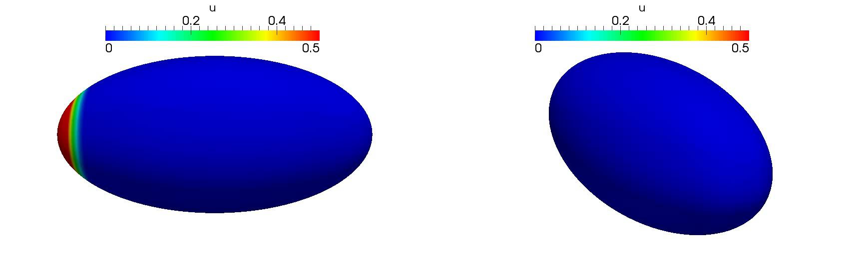
(a) t=0

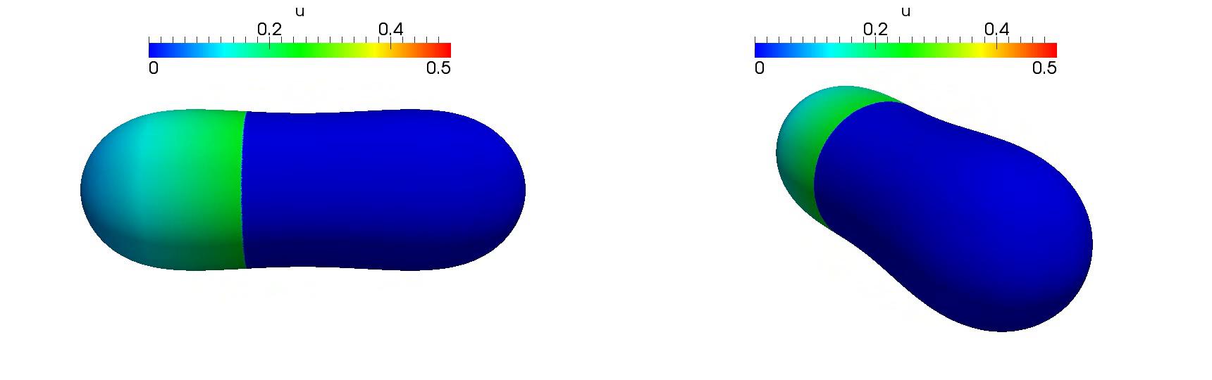
(b) t=0.2T

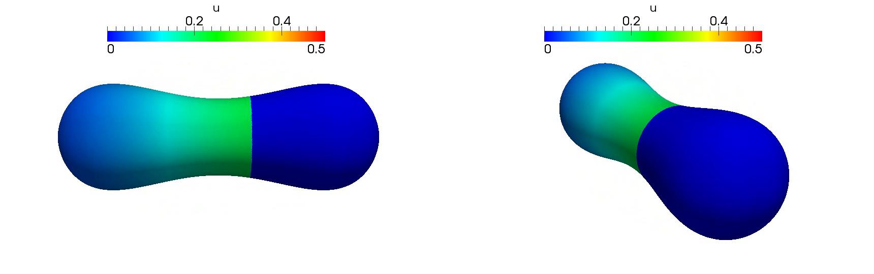
(c) t=0.4T

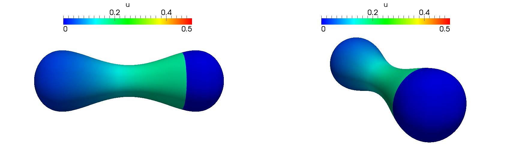
(d) t=0.6T

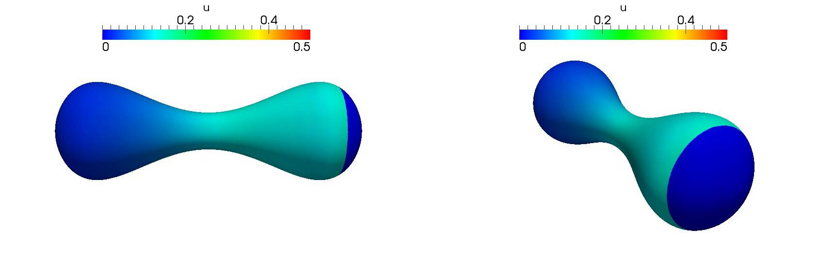
(e) t=0.8T

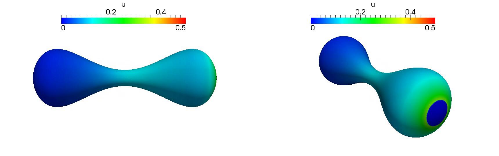
(f) t=T

Figure 1. Burgers like shock on an evolving ellipsoid for several time steps. Here, $T$ denotes the end time.

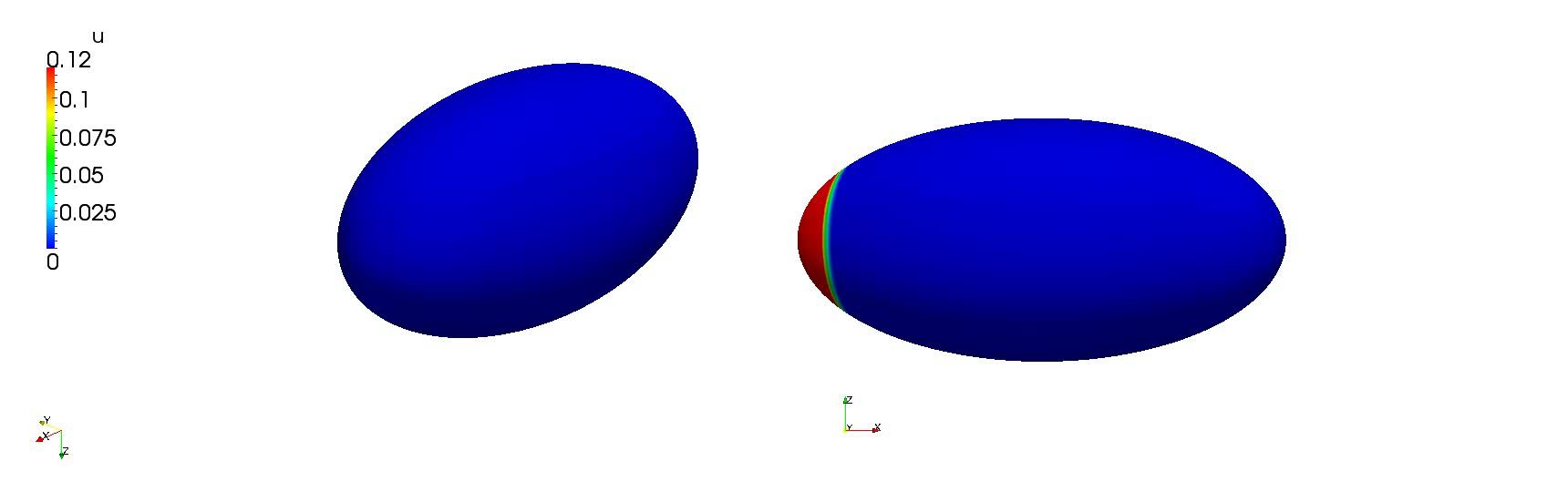
(a) t=0

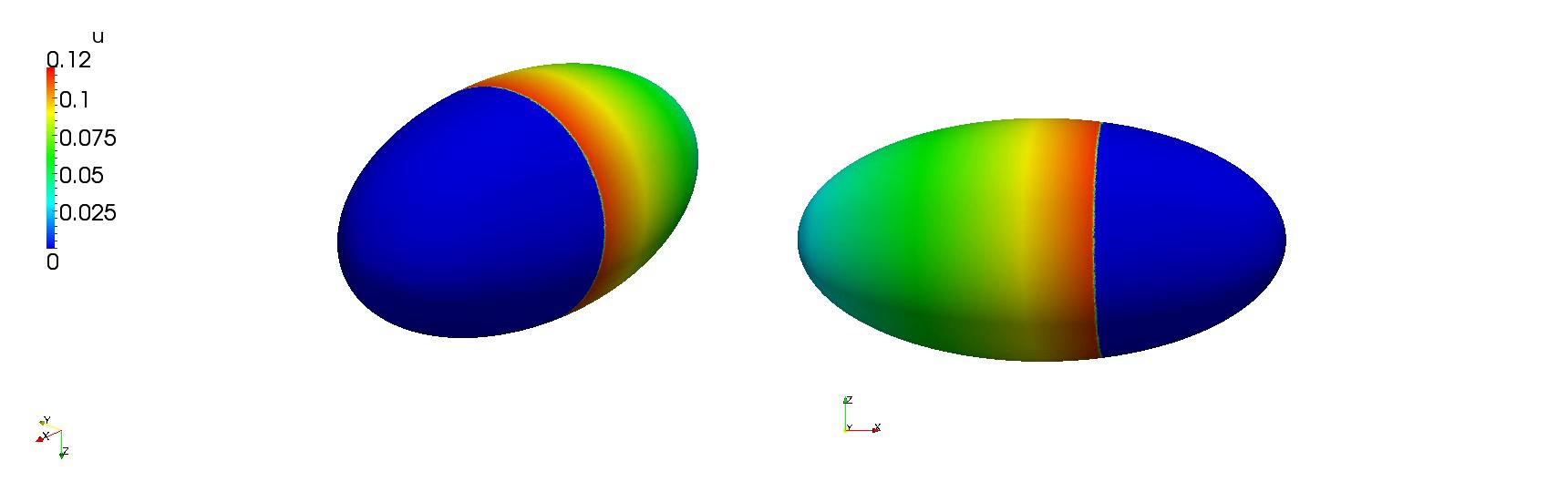
(b) t=0.40T

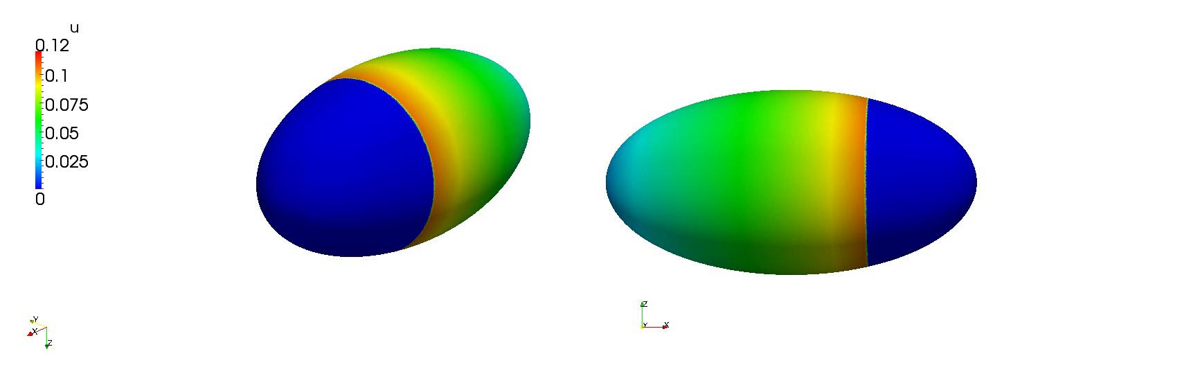
(c) t=0.50T

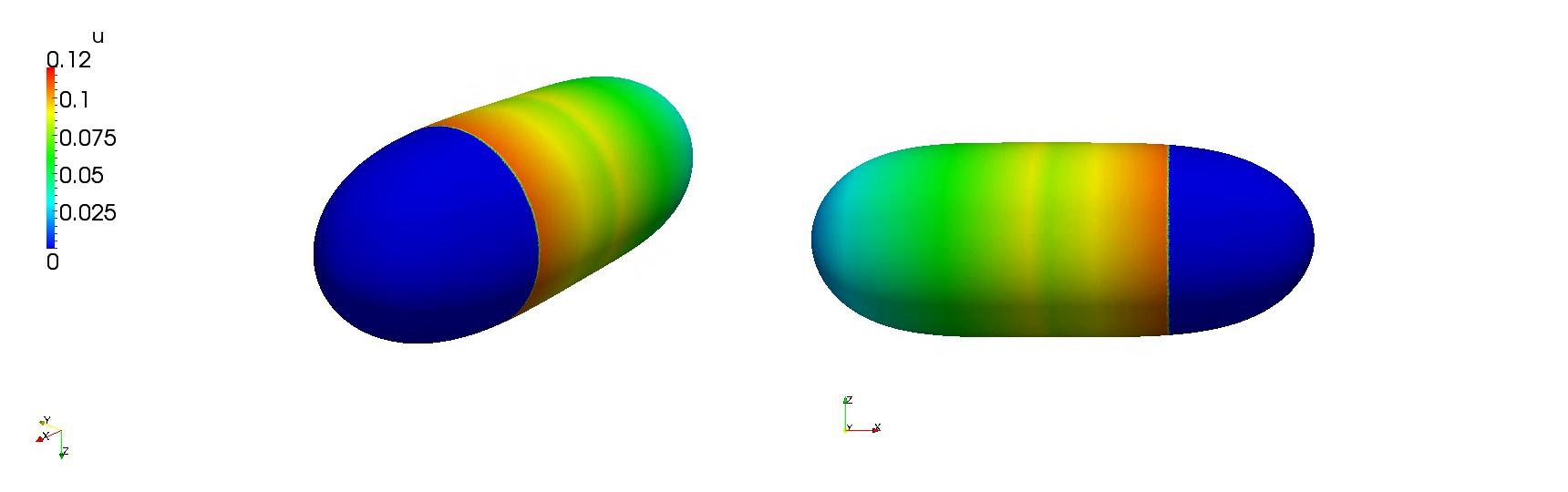
(d) t=0.54T

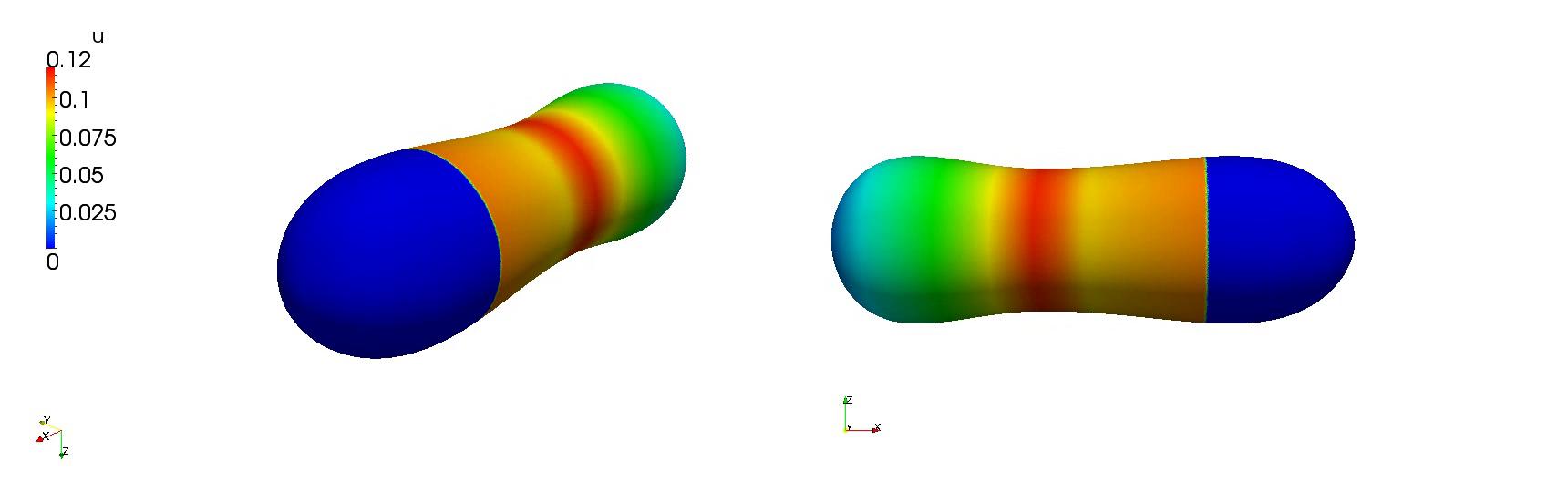
(e) t=0.58T

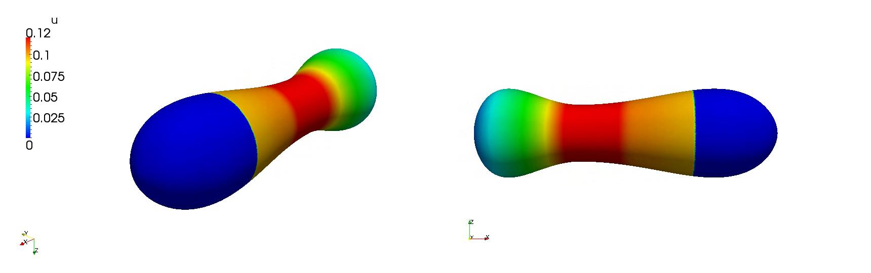
(f) t=0.62T

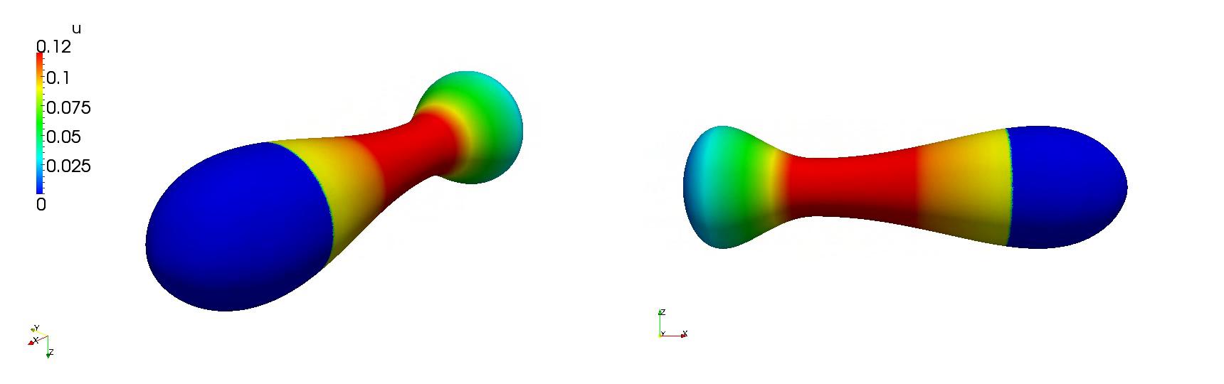
(g) t=0.67T

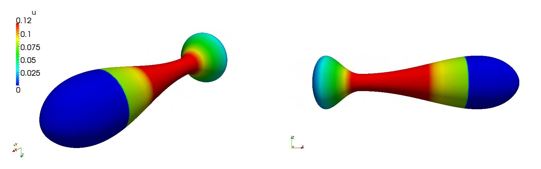
(h) t=0.73T

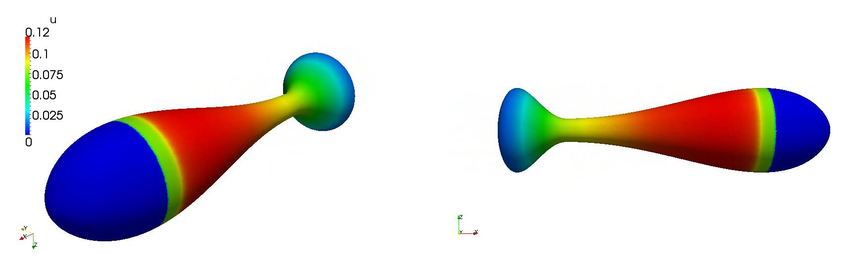
(i) t=0.91T

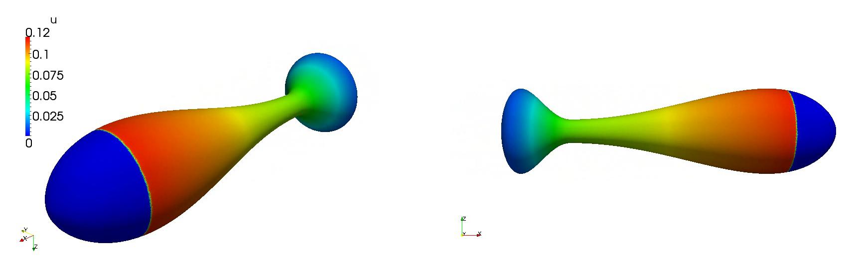
(j) t=T

Figure 2. We see a Burgers like shock on an evolving ellipsoid. Caused by the deformation of the ellipsoid a second shock is produced and overtakes the first one. Here, $T$ denotes the end time.

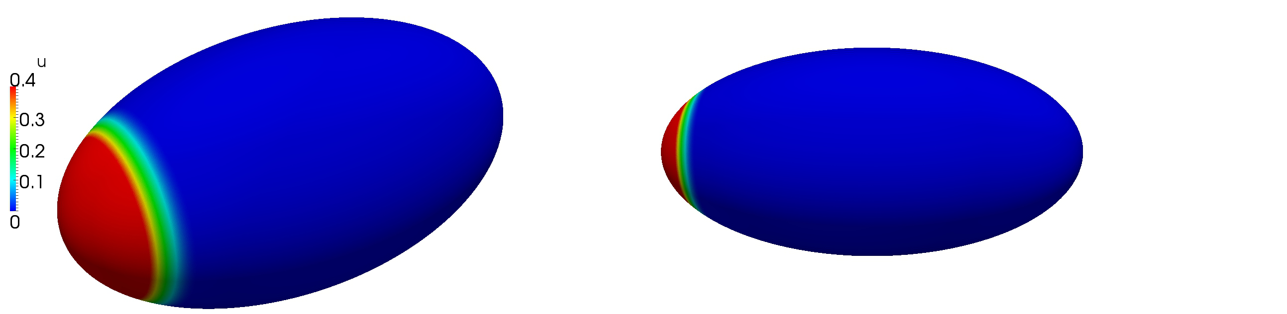
(a) t=0

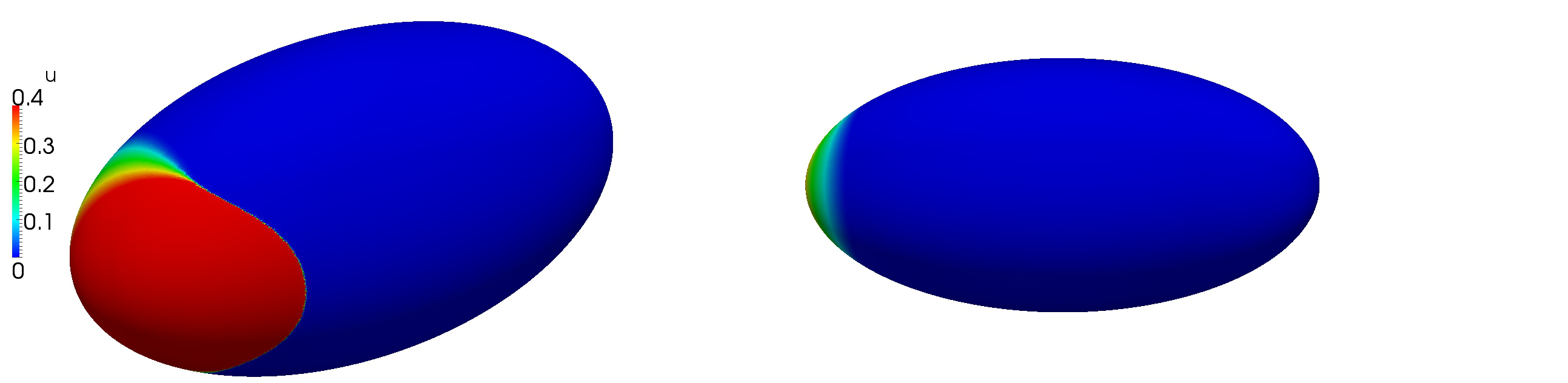
(b) t=0.02T

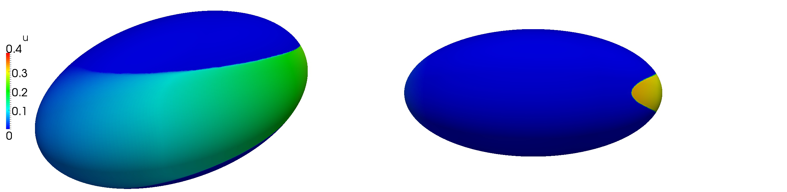
(c) t=0.22T

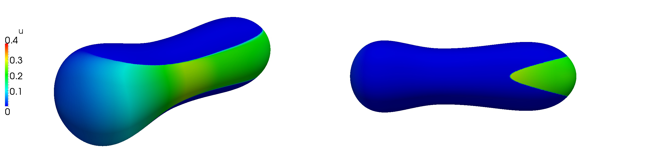
(d) t=0.26T

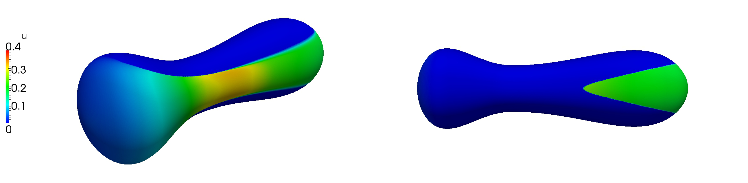
(e) t=0.28T

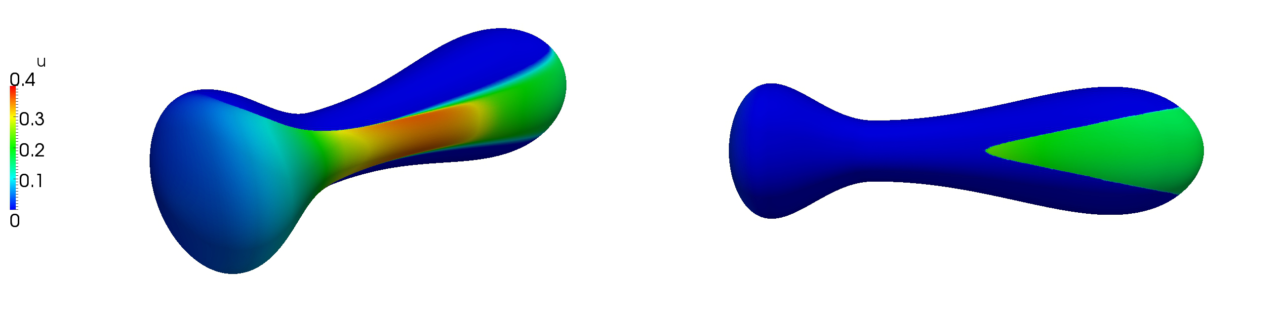
(f) t=0.29T

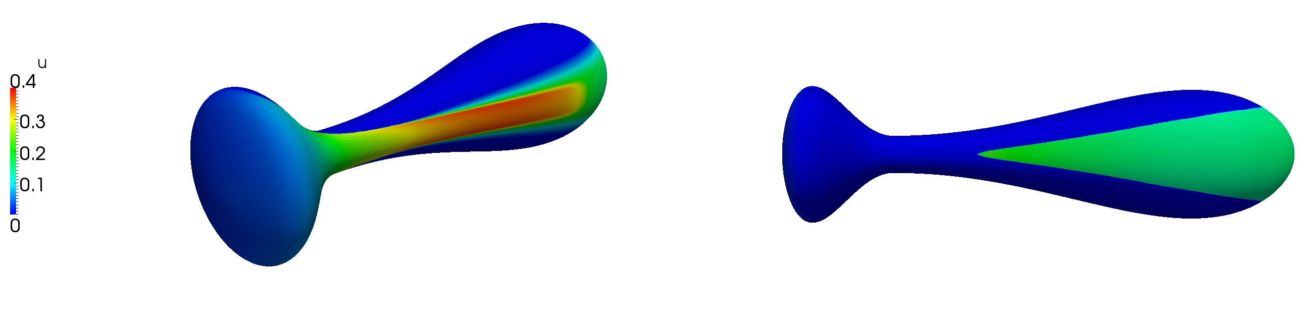
(g) t=0.33T

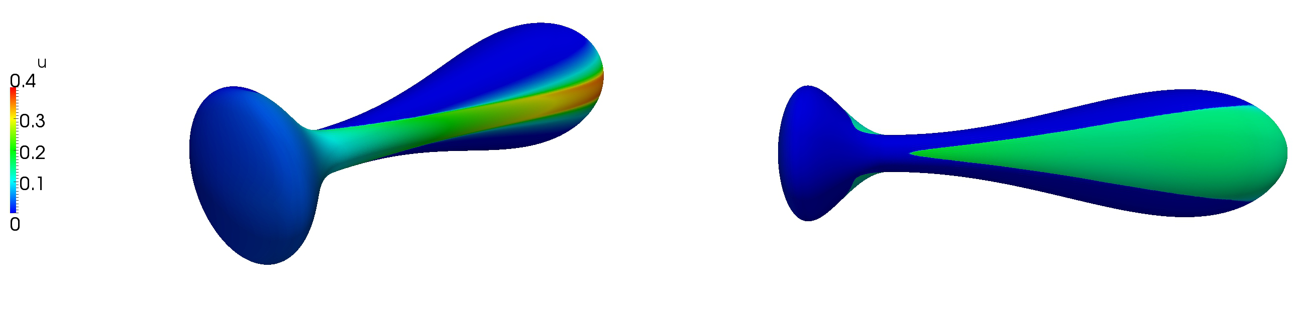
(h) t=0.40T

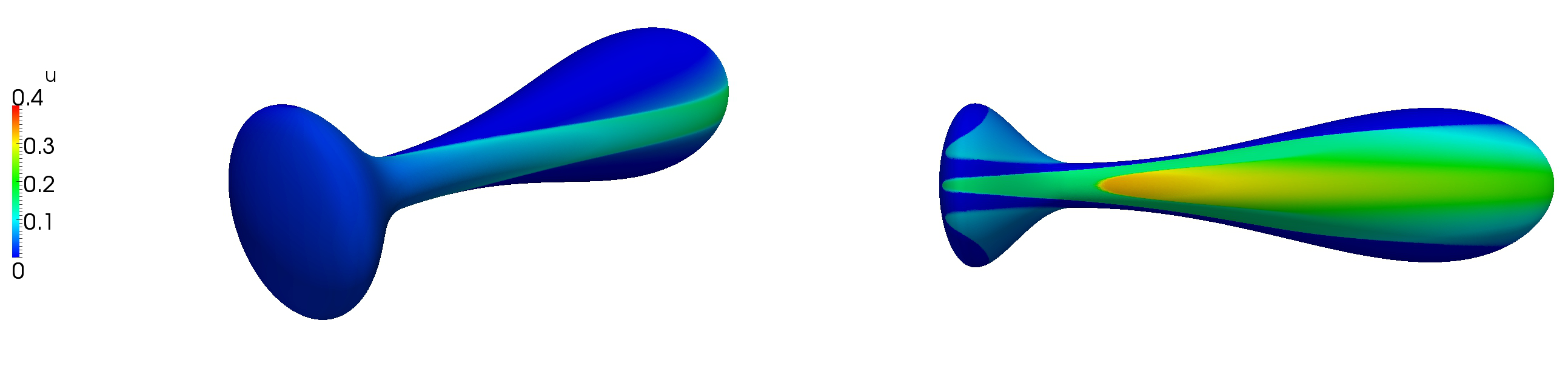
(i) t=0.58T

(j) t=0.64T

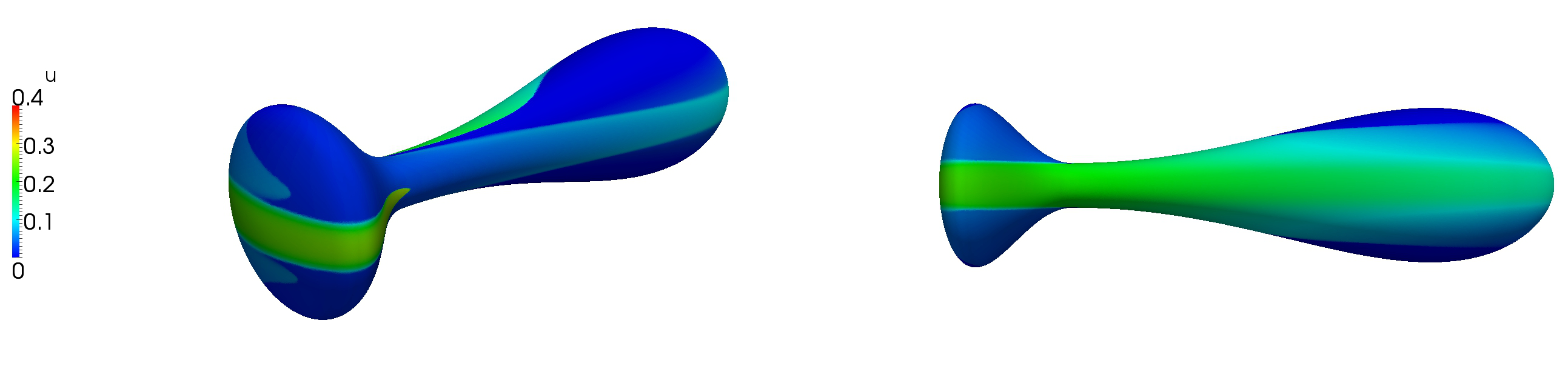
(k) t=0.79T

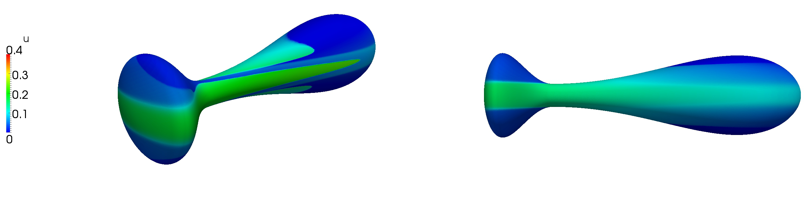
(l) t=T

Figure 3. As in Figure 2 a second shock is geometrically induced and overtakes the first one. Here, the flux function $f$ is divrgence-free. $T$ denotes the end time.

12. Appendix

Proof of Lemma 2.6

Proof.

It is sufficient to prove this relation locally. For this we use a parametrization $X=X(\theta,t)$, $\theta\in\mathcal{O}$ over some open set $\mathcal{O}\subset\mathbb{R}^{n}$. We write $U(\theta,t)=u(X(\theta,t),t)$ and $V(\theta,t)=v(X(\theta,t),t)$. We use the notation $g_{ij}=X_{\theta_{i}}\cdot X_{\theta_{j}}$. The uppering of the indices have to be understood in the usual sense as inverting the matrix: $(g^{ij})_{i,j=1,\dots,n}=(g_{ij})_{i,j=1,\dots,n}^{-1}$.

Then, by definition of the material derivative (7) we have

$$\left(\underline{D}_{l}u\right){\dot{\leavevmode\nobreak\ }}\circ X=\frac{\partial}{\partial t}\left(\underline{D}_{l}u\circ X\right)=\frac{\partial}{\partial t}\left(g^{ij}U_{\theta_{j}}X^{l}_{\theta_{i}}\right)$$

$$=\frac{\partial g^{ij}}{\partial t}U_{\theta_{j}}X^{l}_{\theta_{i}}+g^{ij}U_{t\theta_{j}}X^{l}_{\theta_{i}}+g^{ij}U_{\theta_{j}}X^{l}_{t\theta_{i}}$$

We have that $U_{t}=\dot{u}\circ X$ and $X_{t}=V=v\circ X$. With the relation

$$g^{ij}_{t}=-g^{ik}g^{jm}\left(V_{\theta_{k}}\cdot X_{\theta_{m}}+X_{\theta_{k}}\cdot V_{\theta_{m}}\right)$$

we get

$$\left(\underline{D}_{l}u\right)^{\dot{\leavevmode\nobreak\ }}\circ X=-g^{ik}g^{jm}\left(V^{r}_{\theta_{k}}X^{r}_{\theta_{m}}+X^{s}_{\theta_{k}}V^{s}_{\theta_{m}}\right)U_{\theta_{j}}X^{l}_{\theta_{i}}+g^{ij}U_{t\theta_{j}}X^{l}_{\theta_{i}}+g^{ij}U_{\theta_{j}}X^{l}_{t\theta_{i}}$$

$$=-g^{ik}V^{r}_{\theta_{k}}X^{l}_{\theta_{i}}g^{jm}X^{r}_{\theta_{m}}U_{\theta_{j}}-g^{ik}X^{s}_{\theta_{k}}X^{l}_{\theta_{i}}g^{jm}V^{s}_{\theta_{m}}U_{\theta_{j}}+g^{ij}U_{t\theta_{j}}X^{l}_{\theta_{i}}+g^{ij}U_{\theta_{j}}V^{l}_{\theta_{i}}$$

$$=-\underline{D}_{l}uv_{r}\circ X\underline{D}_{r}u\circ X-\underline{D}_{s}x_{l}\circ X\nabla_{\Gamma}v_{s}\cdot\nabla_{\Gamma}u\circ X+\underline{D}_{l}\dot{u}\circ X+\nabla_{\Gamma}u\cdot\nabla_{\Gamma}v_{l}\circ X.$$

Because of $\underline{D}_{s}x_{l}=P_{sl}=\delta_{sl}-\nu_{s}\nu_{l}$ we finally arrive at

$$\left(\underline{D}_{l}u\right){\dot{\leavevmode\nobreak\ }}=\underline{D}_{l}\dot{u}-\underline{D}_{l}v_{r}\underline{D}_{r}u-P_{sl}\underline{D}_{r}v_{s}\underline{D}_{r}u+\underline{D}_{r}u\underline{D}_{r}v_{l}$$

$$=\underline{D}_{l}\dot{u}-\underline{D}_{r}u\left(\underline{D}_{l}v_{r}+P_{sl}\underline{D}_{r}v_{s}-\underline{D}_{r}v_{l}\right).$$

The Lemma is proved. ∎

References

- [1] P. Amorim, M. Ben-Artzi, and P. G. LeFloch. Hyperbolic conservation laws on manifolds: total variation estimates and the finite volume method. Methods Appl. Anal. 12(3): 291–323, 2005.
- [2] P. Amorim, P. G. LeFloch, and W. Neves. A geometric approach to error estimates for conservation laws posed on a spacetime. Preprint http://arxiv.org/abs/1002.3137
- [3] T. Aubin. Nonlinear analysis on manifolds: Monge-Ampère equations. Reihe Grundlehren der Mathematischen Wissenschaften [Fundamental Principles of Mathematical Sciences], Band 252, 1982.
- [4] D. S. Bale. Wave propagation algorithms on curved manifolds with applications to relativistic hydrodynamics. Thesis.
- [5] M. J. Berger, D. A. Calhoun, C. Helzel, and R. J. LeVeque. Logically rectangular finite volume methods with adaptive refinement on the sphere. Philos. Trans. R. Soc. Lond. Ser. A Math. Phys. Eng. Sci. 367(1907): 4483–4496, 2009.
- [6] M. Ben-Artzi, J. Falcovitz, and P. G. LeFloch. Hyperbolic conservation laws on the sphere: a geometry-compatible finite volume scheme. J. Comput. Phys., 228(16):5650–5668, 2009.
- [7] M. Ben-Artzi, and P. G. LeFloch. Well-posedness theory for geometry-compatible hyperbolic conservation laws on manifolds. Ann. Inst. Henri Poincaré, Anal. Non Linéaire, 24(6):989–1008, 2007.
- [8] D. A. Calhoun, C. Helzel, and R. J. LeVeque. Logically rectangular grids and finite volume methods for PDEs in circular and spherical domains. SIAM Review, 50:723–752, 2008.
- [9] C. M. Dafermos. Hyperbolic conservation laws in continuum physics. Grundlehren der Mathematischen Wissenschaften [Fundamental Principles of Mathematical Sciences], 325, 2010.
- [10] K. Deckelnick, G. Dziuk, and C. M. Elliott. Computation of geometric partial differential equations and mean curvature flow. Acta Numerica, 14:139–232, 2005.
- [11] G. Dziuk, and C. Elliott. Finite elements on evolving surfaces. IMA Journal Numerical Analysis, 25:385–407, 2007.
- [12] G. Dziuk, and C. Elliott. -estimates for the evolving surface finite element method. (to appear in Math. Comp.).
- [13] G. Dziuk, and C. Elliott. A fully discrete evolving surface finite element method. (submitted to SINUM).
- [14] G. Dziuk, and C. Elliott. Fully discrete evolving surface finite element method. (submitted to SIAM J. Numer. Anal.).
- [15] G. Dziuk, C. Lubich, and D. Mansour. Runge–Kutta time discretization of parabolic differential equations on evolving surfaces. IMA J. Numer. Anal., doi:10.1093/imanum/drr017, 2011.
- [16] J. Giesselmann. A convergence result for finite volume schemes on Riemannian manifolds. Math. Model. Numer. Anal., 43(5):929–955, 2009.
- [17] D. Gilbarg, and N. S. Trudinger. Elliptic partial differential equations of second order. Springer Berlin Heidelberg, 2001.
- [18] K. Hermsdörfer, C. Kraus, and D. Kröner. Interface conditions for limits of the Navier-Stokes-Korteweg modell. Interfaces Free Bound. 13:239–254, 2011.
- [19] N. Jung, B. Haasdonk, and D. Kröner. Reduced basis method for quadratically nonlinear transport equations. Int. J. Computing Science and Mathematics, 2:334–353, 2009.
- [20] D. Kröner, and T. Müller. Related problems for TV-estimates for conservation laws on surfaces. accepted for Hyperbolic problems. Theory, numerics and applications. Proceedings of the 13th international conference on hyperbolic problems, 2010, Peking, 2010.
- [21] D. Kröner. Jump conditions across phase boundaries for the Navier-Stokes Korteweg system. accepted for Hyperbolic problems. Theory, numerics and applications. Proceedings of the 13th international conference on hyperbolic problems, 2010, Peking, 2010.
- [22] D. Kröner. Numerical schemes for conservation laws. Wiley-Teubner Series Advances in Numerical Mathematics. John Wiley & Sons Ltd., Chichester, 1997.
- [23] S. N. Kružkov. First order quasilinear equations with several independent variables. Mat. Sb. (N.S.), 81(123):228–255, 1970.
- [24] P. G. LeFloch, and J. M. Stewart. Shock waves and gravitational waves inmatter spacetimes with Gowdy symmetry. Portugalieae Mathematica, 62, Fasc. 3, Nova Serie, 2005.
- [25] P. G. LeFloch, W. Neves, and B. Okutmustur. Hyperbolic conservation laws on manifolds. Error estimate for finite volume schemes. Acta Math. Sin., Engl. Ser., 25(7):1041–1066, 2009.
- [26] D. Lengeler, and T. Mueller. Scalar conservation laws on constant and time-dependent Riemannian manifolds. Preprint.
- [27] M. Lenz, S. F. Nemadjieu, and M. Rumpf. A convergent finite volume scheme for diffusion on evolving surfaces. SIAM Journal on Numerical Analysis, 49(1):15–37, 2011.
- [28] T. Müller. Erhaltungsgleichungen auf Mannigfaltigkeiten Wohlgestelltheit, Totalvariationsabschätzungen und Numerik. Diplomarbeit, Freiburg, 2010.
- [29] J. A. Rossmanith. A wave propagation method with constrained transport for ideal and shallow water magnetohydrodynamics. Thesis.
- [30] J. A. Rossmanith, D. S. Bale, and R. J. LeVeque. A wave propagation algorithm for hyperbolic systems on curved manifolds. J. Comput. Phys., 199:631–662, 2004.