Turbulent pattern formation and diffusion in the early-time dynamics
in the relativistic heavy-ion collision

Abstract

We propose a picture of turbulent pattern formation in the relativistic heavy-ion collision, which follows an efficient process to break color strings and dispose energy in the whole phase space. We perform numerical simulations using the SU(2) pure Yang-Mills theory in a non-expanding box to observe a dynamical phenomenon in the transverse plane akin to the domain growth in time-dependent spin systems.

I Introduction

Relativistic heavy-ion collision experiments at RHIC in BNL and at LHC in CERN have successfully created a quark-gluon plasma and probed into its detailed properties; among milestones in the quark-gluon plasma research, the recognition of the so-called perfect fluidity, i.e. smallness of the shear viscosity to the entropy density ratio was the most influential one, which has triggered interdisciplinary discussions over many fields including nuclear physics and super-string theories.

Thanks to the tremendous developments of the lattice simulation of quantum chromodynamics (QCD) Philipsen:2012nu and the (dissipative) hydrodynamic model Hirano:2012kj , we have reached a reasonable understanding on the static properties of high-$T$ QCD matter and the subsequent dynamical evolution. It is, however, still far from establishing a firm theoretical framework for the pre-thermalization stage. Generally speaking, the thermalization process out of equilibrium is a ubiquitous but complicated problem, and theoretical research mostly relies on numerical methods.

Luckily, in the case of the relativistic heavy-ion collision at high enough energy, the very early-time dynamics at the time scale of order of $\tau\sim Q_{s}\lesssim 0.1\text{fm}/c$ can be expressed in terms of coherent gluon fields, where $Q_{s}$ is the saturation momentum Iancu:2002xk . The initial state characterized by $Q_{s}$ is sometimes referred to as the “glasma” initial condition Lappi:2006fp . In this glasma picture the most important is the presence of boost-invariant longitudinal chromo-electric and chromo-magnetic fields, $\mathcal{E}^{\eta}$ and $\mathcal{B}^{\eta}$, the intensity of which is given by $Q_{s}$ again.

In contrast to the glasma stage, the time scale when the hydrodynamic model starts working is of order $\tau\lesssim 1\text{fm}/c$. It is an urgent theoretical problem to fill in the gap between these times scales. Along this line there are many theoretical attempts based on the glasma simulation Romatschke:2005pm ; Fujii:2008dd ; Fukushima:2011nq , the plasma instability Mrowczynski:1993qm , the hard-loop expansion Mrowczynski:2004kv , the kinetic description Bratkovskaya:2000qy , the holographic duals Janik:2006gp ; Chesler:2008hg , and the classical Yang-Mills simulations Muller:1992iw ; Berges:2007re .

In this work we solve the Yang-Mills equation of motions starting with the glasma initial condition. The question is then; what is the most likely candidate for the mechanism to “decohere” the longitudinal $\mathcal{E}^{\eta}$ and $\mathcal{B}^{\eta}$ in such a short time scale. This kind of decoherence problem is a quite generic problem we may encounter in various circumstances (see e.g. Dusling:2010rm for a scalar-model study). Our proposal is that the turbulent diffusion should be the driving force for this; indeed it is known in many physical phenomena that the turbulence is a much faster process than the typical molecular diffusion by several orders of magnitude.

In the context of the RHIC and LHC physics, the role of the turbulence has been emphasized as a possible account for the smallness of the viscosity to the entropy density ratio Asakawa:2006tc – because the energy transport goes efficiently, an anomalously small viscosity arises generally in a turbulent flow. The actual calculation assumes a random background distribution of chromo-fields Kirakosyan:2012aq . Therefore, we still need to consider from where these fields are generated, and the glasma simulation is indispensable to answer such a question. The turbulence, especially the wave turbulence, has also been investigated numerically and analytically Berges:2008mr ; Schlichting:2012es ; Kurkela:2012hp ; Berges:2013eia . It has been understood that the Kolmogorov-type cascade leads to a power-law spectrum (where the power index may take different values at strong coupling). The Kolmogorov behavior is, however, realized in a system with a well-developed inertial region Zakharov . This means that we have to wait for a certain time until the power-law spectrum grows steadily, while what we want to clarify is not the steadiness but the rapid reorganization from the initial state. We should, hence, disturb the initial system with substantially large fluctuations that breach the boost invariance.

For this purpose, in this work, we turn off the effect of the expanding geometry. We do this because the expanding geometry is singular at the initial time and it is difficult to disturb the initial state without ambiguity. Besides, the expansion quickly renders the transverse dynamics frozen, and thus, one should carefully formulate the initial spectral shape (involving the UV divergence) and also elaborate the proper renormalization (or subtraction) procedures Dusling:2010rm ; Fukushima:2006ax . Otherwise, useful information on underlying physics can be easily diluted and even concealed by the effect of expansion. These are not simply technical problems; the expanding geometry represents curved space-time and quantum fluctuations on such curved space-time are distorted, so that the physical vacuum should be Bogoliubov transformed from the vacuum in flat space-time. Interestingly enough, as we will find later, a particular initial condition corresponding to the heavy-ion collision already captures the essential features of the anisotropic dynamics. Moreover, we have checked whether we can confirm the same observation using a code for the expanding case, and have found similar behavior if we employ large fluctuations, while the non-expanding simulation always leads to inhomogeneous pattern formation for any (small) fluctuations.

One might feel that the approximation to adopt a non-expanding box be artificial simplification. However, it is just obvious that the expansion effects should delay the decohering processes, and therefore, one must first understand the decohering mechanism for the non-expanding system; otherwise it is impossible to give any account for the expanding case. Then, one should test the presumed mechanism to see whether it works to overcome the delay in the expanding case. This is why we dare to drop the expansion off; the relevance to the experiment becomes less, but the theory becomes more well-behaved thanks to this simplification.

The most important point in this work is that the longitudinal and the transverse dynamics behave totally differently at early time when the anisotropy from the collision geometry is huge. One can presume by intuition that the longitudinal decoherence should go much faster than the transverse one; otherwise the isotropization is never achieved. Indeed we will confirm this anticipation, and find that it indeed happens in a very interesting manner.

II Formulation

Most importantly, we can make use of the glasma initial condition Kovner:1995ja ; Krasnitz:1998ns as it is even in the non-expanding case because the initial fields lie only on the transverse plane. In terms of the link variables on the lattice, the canonical momenta leads to the following time evolution,

$$U_{i}(t+2\Delta t)=\exp\bigl{[}-igE^{i}(t+\Delta t)\cdot 2\Delta t\bigr{]}U_{i}(t)\;,$$ (1)

where the time arguments are shifted in accord to the leapfrog algorithm which preserves the Gauss law exactly. We omit writing the lattice spacing $a$ throughout this paper. The classical Yang-Mills equations of motion (Hamilton’s equations) read,

$$\begin{split}&E^{i}(t+\Delta t)-E^{i}(t-\Delta t)\\ &\qquad=2\Delta t\cdot\frac{i}{2g}\sum_{j\neq i}\bigl{[}U_{ji}(t)+U_{-ji}(t)-\text{(h.c.)}\bigr{]}\end{split}$$ (2)

in the temporal axial gauge; $U_{t}=1$. The initial condition is given in a standard way, which simplifies particularly for the SU(2) color group Krasnitz:1998ns as

$$U_{i} =\bigl{(}U_{i}^{(1)}+U_{i}^{(2)}\bigr{)}\bigl{(}U_{i}^{(1)\dagger}+U_{i}^{(2)\dagger}\bigr{)}^{-1}\;,$$ (3)

$$E^{z} =\frac{-i}{4g}\sum_{i=x,y}\Bigl{\{}(U_{i}\!-\!1)\bigl{(}U_{i}^{(2)\dagger}\!+\!U_{i}^{(1)\dagger}\bigr{)}+\bigl{[}U_{i}^{\dagger}(x\!-\!\Delta x_{i})\!-\!1\bigr{]}$$

$$\quad\times\bigl{[}U_{i}^{(2)\dagger}(x\!-\!\Delta x_{i})\!-\!U_{i}^{(1)\dagger}(x\!-\!\Delta x_{i})\bigr{]}-\text{(h.c.)}\Bigr{\}}$$ (4)

with the pure gauge configurations, $U_{i}^{(m)}(\boldsymbol{x}_{\perp})=V^{(m)}(\boldsymbol{x}_{\perp})V^{(m)\dagger}(\boldsymbol{x}_{\perp}\!+\!\Delta x_{i})$, and the gauge rotation, $V^{(m)\dagger}=e^{ig\Lambda^{(m)}}$, by the static potential obtained as a solution of the Poisson equation, $\partial_{\perp}^{2}\Lambda^{(m)}=-\rho^{(m)}$.

We assume the Gaussian distribution for the color source; $\langle\rho^{(n)}(\boldsymbol{x}_{\perp})\rho^{(m)}(\boldsymbol{x}_{\perp}^{\prime})\rangle\!=\!\delta^{nm}g^{2}\mu^{2}\delta(\boldsymbol{x}_{\perp}\!-\!\boldsymbol{x}_{\perp}^{\prime})$, where $\mu$ is supposed to be related to the characteristic scale $Q_{s}$ as was mentioned in the previous section. If we solved the time evolution with the initial condition (3) and (4), there would appear no dependence on the longitudinal coordinate (i.e. $z$ in the present case without expansion, corresponding to $\eta$ in the Bjorken coordinates). This means that QCD color strings extend along the $z$-direction at initial time. We shall introduce a minimal perturbation to make it the clearest how these strings are disrupted by extra fluctuations;

$$E^{i}=g^{3}\mu^{2}[f(z\!-\!\Delta z)-f(z)]\xi^{i}\;,~{}~{}f(z)=\Delta\cos(2\pi z/L_{z})\;,$$ (5)

where $\langle\xi^{i}(\boldsymbol{x}_{\perp})\xi^{j}(\boldsymbol{x}_{\perp}^{\prime})\rangle=\delta^{ij}\delta^{(2)}(\boldsymbol{x}_{\perp}\!-\!\boldsymbol{x}_{\perp}^{\prime})$ and $\delta E^{\eta}$ solved from the Gauss law. In this way we put a seed of electric-field amplitude $\propto\Delta$ at the lowest non-zero momentum $|k_{z}^{\text{(min)}}|=2\pi/L_{z}$. As long as the instability stays weak, the linear superposition gives a good approximation for the results with more general fluctuations Fukushima:2011nq . In this work, however, we will also choose a non-small $\Delta$ to test the robustness of what we discover. In principle, we should generate the quantum fluctuations according to the ground state (Gaussian) wave-function, and take the ensemble average over all fluctuations, which would lead to the UV divergence of the zero-point oscillation energy. To avoid this complication, in this work, we pick up a “representative” of the configuration by Eq. (5). This simplification would affect quantitative details such as the precise time scale of the decoherence, but should be harmless to the qualitative nature of the phenomenon that we will discuss.

III Numerical Results

First let us address the case without $z$-dependent fluctuations. With unbroken translational invariance in the $z$-direction, the transverse pressure $P_{\text{T}}$ approaches a finite value, while the longitudinal pressure $P_{\text{L}}$ decreases to vanish asymptotically, where they are, respectively, defined as

$$P_{\text{L}}=\text{tr}\bigl{[}(E^{x})^{2}\!+\!(E^{y})^{2}\!-\!(E^{z})^{2}\!+\!(B^{x})^{2}\!+\!(B^{y})^{2}\!-\!(B^{z})^{2}\bigr{]}\;,$$

$$P_{\text{T}}=\text{tr}\bigl{[}(E^{z})^{2}+(B^{z})^{2}\bigr{]}\;.$$ (6)

In our numerical computation we use $g^{2}\mu=120/L_{\perp}$ (corresponding to the choice $g^{2}\mu\sim 2\,\text{GeV}$) with $g=2$ and the transverse and longitudinal site numbers, $L_{\perp}=L_{z}=96$. We note that the initial energy density is both UV and IR singular Kovchegov:2005ss :

$$\varepsilon(t=0)=N_{\text{c}}(N_{\text{c}}^{2}-1)\frac{(g^{2}\mu)^{4}}{8\pi^{2}g^{2}}\biggl{[}\ln\frac{\Lambda_{\rm UV}}{m_{\rm IR}}\biggr{]}^{2}\;,$$ (7)

where $\Lambda_{\rm UV}$ and $m_{\rm IR}$ are UV and IR cutoff scales, respectively. This singularity is problematic in a non-expanding box, while the time evolution soon diminishes this singularity in the expanding case Kovchegov:2005ss . In our numerical simulation, thus, we need to introduce a UV cutoff $(k_{\perp})_{\rm max}$ when we solve the Poisson equation, i.e. higher modes with $k_{\perp}>(k_{\perp})_{\rm max}=32\cdot 2\pi/L_{\perp}\sim 1.7g^{2}\mu\sim 3.4\,\text{GeV}$ are dropped to get the results presented in this paper. We have then confirmed that our results have only minor dependence on $L_{\perp}$ as long as we keep the same $(k_{\perp})_{\rm max}$. We also note that, because of the color string, the initial $P_{\text{L}}$ starts from a negative value (i.e. two nuclei feel an attractive force).

It is already a non-trivial observation that $P_{\text{L}}$ vanishes at late time. In the expanding case, since the system is stretched and diluted, one may anticipate $P_{\text{L}}\to 0$ as a result of the free streaming. In the present simulation, however, the box does not expand and nothing streams out, so that $P_{\text{L}}\to 0$ is purely realized by the choice of the initial conditions (3) and (4). This implies that $P_{\text{L}}\to 0$ even in the expanding glasma should be attributed to not the expansion but the initial conditions. In other words, the free streaming is not the reason, but the physical interpretation of the result.

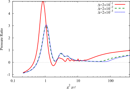
Figure 1: Pressure ratio $P_{\text{L}}/P_{\text{T}}$ as a function of dimensionless time. Without fluctuation the ratio approaches zero, while it goes to a non-zero constant if fluctuations are implemented. An ensemble average is taken over 50 configurations.

We shall next proceed to the results with $z$-disturbing fluctuations, as shown in Fig. 1. We here adopt three different $\Delta$; a substantially large $\Delta=0.2$ gives the energy density from fluctuations of the same order of magnitude as the background fields. Therefore, this value is a kind of upper bound above which solving the classical equations of motion is no longer justified. A marginal $\Delta=0.02$ is much safer; the initial energy density is dominated by the background fields, and the time evolution is almost identical with the case with even smaller $\Delta=0.002$, as is manifested in Fig. 1. (To avoid making the figure too busy, we did not show the fluctuation-free results with $\Delta=0$ that behave like the results with $\Delta=0.02$ or $0.002$ till $g^{2}\mu t\sim 60$, and monotonically approach zero beyond it.)

There are two interesting observations that one can notice at a glance. First, the choices of $\Delta=0.02$ and $\Delta=0.002$ make only little change in the onset of the instability around $g^{2}\mu t\sim 100$ where $P_{\text{L}}/P_{\text{T}}$ start growing. Owing to this, we can be so sure that our results should be robust at least on a qualitative level regardless of our ignorance about the precise value of $\Delta$. Second, if $\Delta$ is less than $\sim 0.2$, we cannot reach the complete isotropization. This is quite unexpected: Because the simulation runs in the isotropic setup, the anisotropy given at the initial time should naturally fade out if we wait for a sufficiently long time. This intuition is correct, but the point is that it takes an extraordinarily long time unless $\Delta$ is such large that it also modifies the initial energy density. It is quite instructive to see that the isotropization at later time is a very slow process even in a non-expanding and symmetric box.

To discuss more microscopic dynamics, we shall split the time evolution into three distinct characteristic regimes as follows.

III.1 Temporarily and spatially oscillatory regime

The pressure has oscillatory behavior in the earliest stage (i.e. $g^{2}\mu t\lesssim 15$ for $\Delta=0.2$ and $g^{2}\mu t\lesssim 50$ for $\Delta=0.02$ as deduced from Fig. 1). The so-called glasma instability must be developing from lower to higher longitudinal modes, but their effects are not yet appreciable in the bulk thermodynamics at zero mode. In the phenomenological sense, the theoretical understanding in this regime is the most crucial issue, while many theoretical efforts had been devoted to rather later-time dynamics. Hence, our central objective in this present paper is to shed light on this oscillatory regime.

Obviously, the equation of state still has fast components in time, which means that the derivative expansion should not work. One cannot therefore apply the hydrodynamic equations to describe the time evolution yet. Then, a natural question arises; what about the spatial structure? Is it already smooth enough or linked somehow to the rough structure in time?

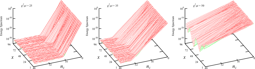
Figure 2: Energy spectrum as a function of the coordinate $x$ (in unit of $a$) and the momentum $k_{z}$ with $y=L_{y}/2$ fixed, calculated for $\Delta=0.02$. The far left represents the result at the initial time $g^{2}\mu t=0.2$, and the time increments up to $g^{2}\mu t=50$ in the right.

To diagnose the microscopic dynamics, we make 3D and density plots to illustrate the cascade flow of the energy spectrum toward higher $k_{z}$ or the wave number $n_{z}$ (where $k_{z}=n_{z}\cdot 2\pi/L_{z}$) in the longitudinal direction. We define the following energy spectrum with only the $z$-direction Fourier transformed as

$$\begin{split}\varepsilon(x,y,k_{z})&=\sum_{i}\text{tr}\bigl{[}E^{i}(x,y,-k_{z})E^{i}(x,y,k_{z})\\ &\qquad\qquad+B^{i}(x,y,-k_{z})B^{i}(x,y,k_{z})\bigr{]}\;,\end{split}$$ (8)

which is measured for each configuration. This is not a gauge invariant quantity and we need to fix the gauge to define it uniquely. We already chose the temporal axial gauge but time-independent gauge rotations are still redundant, which does not change the gauge-invariant observable but modifies $\varepsilon(x,y,k_{z})$. Therefore, we fix the initial gauge configurations (3) and (4) (with fluctuations included) to satisfy the Coulomb-gauge condition $\boldsymbol{\nabla}\cdot\boldsymbol{A}=0$ that would flatten spiky textures. We used the over-relaxation method with 1000 steps to impose the Coulomb gauge and explicitly checked that the gauge configurations become extremely smooth then.

For qualitative discussions we may choose any $\Delta$, in principle, but to remove an impression that our findings come from artificially large $\Delta$, we here adopt a rather safer choice of $\Delta=0.02$ that has no effect on the very early dynamics as is clear from Fig. 1. Then, for graphical purpose, we pick a slice of $y=L_{y}/2$ up and make a 3D plot of $\varepsilon(x,y,k_{z})$ as a function of $x$ and $n_{z}$ in Fig. 2 for one configuration.

We can understand from Fig. 2 what is actually happening on the microscopic level during the oscillatory regime. In this very first stage the energy amplitude spreads toward larger $k_{z}$ triggered by spots localized in $x$ (and $y$) space. These localized spots look like narrow avalanches. Let us here “define” what we really mean by avalanche for clarify.

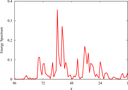
Figure 3: Energy spectrum corresponding to Fig. 2 for $\Delta=0.02$ at $n_{z}=0$ at the initial time $g^{2}\mu t=0.2$ shown in the linear scale.

To do so, we have to magnify the initial energy stored at $n_{z}=0$ mode, which is presented in Fig. 3. It should be noted that this is nothing but the energy distribution already shown in the very left of Fig. 2 in a form of the logarithmic plot. Even though Fig. 3 may look like having a rough structure, the energy fluctuates within only one order of magnitude. It is evident from the right of Fig. 2 that the inhomogeneity developing later at larger $n_{z}$ is correlated to the initial pattern, and the resulting intensity differs by more than ten orders of magnitude! We would call this huge (but relative) amplification of the spatial pattern the avalanche phenomenon.

This type of the avalanche phenomenon is quite common in many physics problems. The avalanche breakdown of insulator or semi-conductor is one familiar example in which free electrons trigger the creation of electron-hole pair. In the present glasma simulation, we have specified both the initial conditions (3), (4), and the initial fluctuations (5) according to the Gaussian distribution, and some local positions happen to have irregular amplitudes as observed in Fig. 3, which is responsible for the avalanches. Probably they have much to do with the magnetic vortices discovered recently in the same model setup Dumitru:2013koh . We here point out that these narrow avalanches are collective consequences from the simultaneous existence of the glasma fields and the fluctuation fields. We turned the glasma background fields off as a test calculation, and we found that the amplitudes just smoothly and slowly decayed into higher $k_{z}$, but no rapid narrow avalanche emerged.

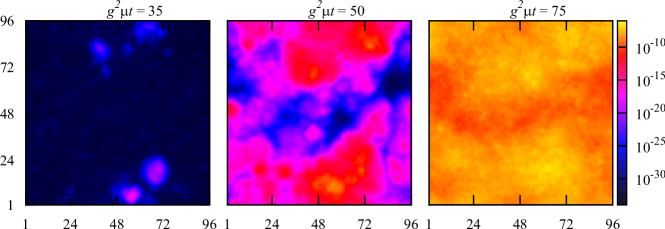
Figure 4: Snapshots of the energy amplitude for $\Delta=0.02$ at maximum $k_{z}$ on the transverse $x$-$y$ plane (in unit of $a$). These are taken at the times corresponding to Fig. 2. Clearly a dynamical pattern is formed first and the region with high $k_{z}$ next spreads over the transverse directions.

These avalanche-like structures gradually spread over $x$ (and $y$) space as the time elapses, and eventually the distribution appears uniform in transverse space at further later time, which we call the transverse diffusion. To access the full transverse structure and visualize the diffusion, we show $\varepsilon(x,y,k_{z})$ as snapshots in Fig. 4 at $g^{2}\mu t=35$, $50$, and $g^{2}\mu t=75$ using the same configuration to draw Fig. 2. We can then clearly perceive the dynamical pattern formation in transverse geometry and subsequent diffusion; at localized spots with brighter colors we have larger amplitudes for the maximum $k_{z}$ mode, namely, $k_{z}^{\text{(max)}}=L_{z}/2\cdot 2\pi/L_{z}=\pi/2$ (in unit of $a^{-1}$). To the best of our knowledge the present analysis is the very first demonstration that has revealed the spontaneous generation of spatial pattern in the real-time simulation of the Yang-Mills theory. At the same time as we emphasize the novelty, we would also like to draw attention to the similarity to many other systems out of equilibrium: One intuitive example lies in the formation of the magnetized domains described by the time-dependent Ginzburg-Landau theory of the classical spin models. Such a pattern has been numerically discovered in the direction from the random initial state to the ordered spin state at lower $T$, and amazingly also in the opposite direction from the enforced ordered (or coherent) state to the disordered (or decoherent) spin state at high $T$ Kudo . Our results are reminiscent of the latter associated with non-equilibrium decohering processes.

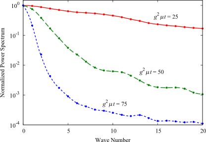
Figure 5: Power spectrum $P(k_{\perp})$ as a function of the transverse wave-number, normalized by the zero-mode value. The ensemble average is taken over 50 configurations.

Let us quantify the transverse diffusion processes by calculating the energy-density correlation function from Fig. 4 or the “power spectrum” defined by

$$P(k_{\perp})=\langle\varepsilon(-k_{\perp},k_{z}^{\text{(max)}})\varepsilon(k_{\perp},k_{z}^{\text{(max)}})\rangle\;,$$ (9)

where we note that the meaning of $k_{\perp}$ is totally different from $k_{z}$; we introduced $k_{\perp}$ as a Fourier transform of $x$ and $y$ of $\varepsilon(x,y,k_{z})$, while $k_{z}$ refers to the momentum carried by the chromo-electric and chromo-magnetic fields.

To absorb orders of magnitude difference at different time, we normalize the power spectrum by the zero-mode value $P(0)$ and draw Fig. 5 for $g^{2}\mu t=25$, $50$, and $75$.

We can clearly confirm that the long-range correlation becomes more and more enhanced as the time goes, which is quite consistent with what we can see from Fig. 4. (We note that the wave-number, say 10 on this plot, corresponds to the physical scale, $10\cdot 2\pi/L_{\perp}\sim 1\,\text{GeV}$.) The reason why the normalized power spectrum seemingly looks more suppressed at larger $g^{2}\mu t$ is that the zero-mode grows larger. Thus the relative height decreases, though the absolute height is much larger at later time. It should be clearly noted here that we should not take this enhancement of the long-range correlation for a signal of the Bose-Einstein condensate speculated as in Blaizot:2011xf . We are now looking at not the particle distribution but the energy-density correlation. We observe that the spots in the transverse plane spread out quickly toward uniformity, which is to be interpreted as the diffusion as can be inferred from Fig. 4.

III.2 Intermediate fast-growing regime

After some time ($15\lesssim g^{2}\mu t\lesssim 30$ for $\Delta=0.2$ and $50\lesssim g^{2}\mu t\lesssim 100$ for $\Delta=0.02$ in Fig. 1) the equation of state behaves smoothly enough in time and also in space, which should enable the hydrodynamic evolution to work fine during this regime since the derivative expansion makes sense. The system still goes on approaching isotropization, and thus it is neither isotropic nor thermalized yet. An important question is what determines the typical time scale for the transition from the oscillatory regime to the growing regime. In other words, we need to know what is still missing to accelerate the onset time for the hydrodynamic evolution. The time scale is characterized by the balance between the initial energy density stored at the zero mode and the rate of the energy flow that is intrinsically determined by the Yang-Mills interactions. Within the present framework it is difficult to yield the onset time around a few times $g^{2}\mu\sim 2\,\text{GeV}\sim 0.1\;\text{fm}/c$ as required by the analysis of the experimental data.

It is important not to be confused with the behavior of the most unstable mode in the expanding case Romatschke:2005pm ; Fukushima:2011nq that looks very similar to Fig. 1. In the expanding case the onset is delayed simply by the kinematical reason Fujii:2008dd , and in the non-expanding case in Fig. 1 it is not the most unstable component but the whole pressure that we are dealing with. Therefore it takes time for the instability to spread over the whole phase space.

III.3 Asymptotic slowly-growing regime

The diffusion is caused by inhomogeneity, and so it becomes slower and slower with less and less inhomogeneity and anisotropy. Naturally the tendency toward isotropization becomes weakened as $P_{\text{L}}$ and $P_{\text{T}}$ get closer to each other. In such an asymptotic regime ($g^{2}\mu t\gtrsim 30$ for $\Delta=0.2$ and $g^{2}\mu t\gtrsim 100$ for $\Delta=0.02$ in Fig. 1) the characteristic time scale is unphysically long. From the experimental point of view, all theoretical considerations in this late regime are irrelevant to the thermalization problem. Nevertheless, as a rather “academic” problem to investigate the non-linear dynamics of the Yang-Mills theory, it is worth paying our attention to microscopic details in this asymptotic regime.

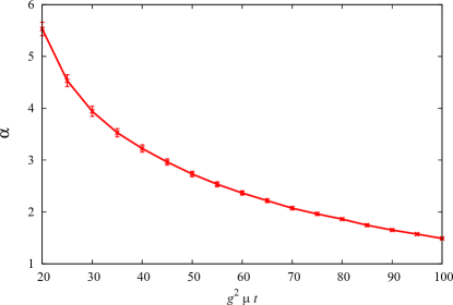
Figure 6: Power index deduced from the tail of the energy spectrum fitted by $k_{z}^{-\alpha}$ given as a function of dimensionless time.

Usually some kind of scaling law may be observed in a well-developed turbulent system at late time. In the present simulation with specific initial conditions (3) and (4), however, the zero mode cannot be a consistent source to supply the energy injection and so it cannot sustain a steady inertial region in the energy spectrum. Still, there may be a chance to see scaling behavior at the tail of the energy spectrum. To test this idea, we attempt to fit the longitudinal energy spectrum by the power-law spectrum $\sim k_{z}^{-\alpha}$, and we find that the fit works well in the range, $n_{z}=25\sim 48$. Then, the power $\alpha$ turns out to be a function of time as in Ref. Schlichting:2012es , which is plotted in Fig. 6. The value of the index $\alpha$ decreases with increasing time, which crosses the Kolmogorov value $5/3=1.67$ and becomes even smaller. As we discussed above, the inertial region is not stable and the precise value of $\alpha$ is not very important in the present case but this level of qualitative agreement is quite suggestive. One might care about the consistency with Ref. Berges:2008mr in which a stable power-law has been identified. We note that this difference between the present analysis and Ref. Berges:2008mr comes from the totally different choice of the initial conditions (3) and (4) that resemble the anisotropy in the heavy-ion collision.

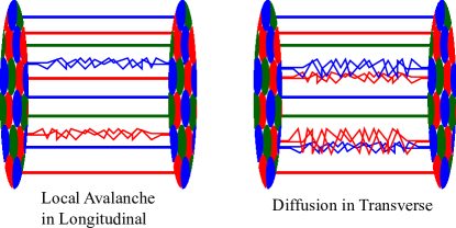
Figure 7: Schematic picture of two fastest processes in the early-time dynamics in the relativistic heavy-ion collision.

IV Conclusions

With the results from our numerical simulations, we can arrive at the following picture of the very early-time stage in the relativistic heavy-ion collision, as is sketched in the illustration of Fig. 7.

The fastest process is driven by the avalanche-like decay along the longitudinal direction which takes place locally in transverse plane. These avalanches are to be attributed to initial fluctuations. Once this occurs, the boost invariance or the $z$-invariance is quickly but only locally broken as in the left of Fig. 7. This view also invokes the famous Reynolds’ experiment of the turbulent flow inside of a pipe reynolds where the translationally steady flow of ink begins wandering under disturbances if Reynolds’ number exceeds a critical point. From this analogy it may well be reasonable to identify these local avalanches as appearance of a sort of fluid turbulence. Also, it would be conceivable to associate them with the QCD string breaking which is accompanied by the particle production.

The next vital fast process is the diffusion over the transverse plane. This turbulent diffusion is a quite efficient mechanism to dispose energy in the whole phase space, and eventually to let the equation of state behave smoothly enough.

Before addressing the possible relevance to the experimental data, the following upgrades should be taken into account: First, it is necessary to incorporate the full quantum spectrum that should further accelerate the process speed. Second, related to this, we should carefully deal with the renormalization and subtract the UV divergence originating from the quantum fluctuation. Third, we need to turn the expansion on, which makes it even more subtle to handle the first and the second points above. In principle, as we commented, the avalanches should be associated with the particle production, which is to be reflected in the moments of the angular distribution of the produced particles. For quantitative theoretical prediction, however, we must tackle the above-mentioned tough obstacles and complete the thermalization scenario first. We believe that the qualitative finding reported in this work should be a crucial step toward solving the puzzle of the thermalization problem.

- (1) For a review on the finite- lattice simulation, see; O. Philipsen, Prog. Part. Nucl. Phys. 70, 55 (2013).
- (2) For a review on the hydrodynamic models, see; T. Hirano, P. Huovinen, K. Murase and Y. Nara, Prog. Part. Nucl. Phys. 70, 108 (2013).
- (3) For reviews on the saturation effect in high-energy QCD, see; E. Iancu, A. Leonidov and L. McLerran, hep-ph/0202270; E. Iancu and R. Venugopalan, In *Hwa, R.C. (ed.) et al.: Quark gluon plasma* 249-3363 [hep-ph/0303204]. L. McLerran, Acta Phys. Polon. B 41, 2799 (2010).
- (4) T. Lappi and L. McLerran, Nucl. Phys. A 772, 200 (2006).
- (5) P. Romatschke and R. Venugopalan, Phys. Rev. Lett. 96, 062302 (2006); Phys. Rev. D 74, 045011 (2006).
- (6) H. Fujii and K. Itakura, Nucl. Phys. A 809, 88 (2008); H. Fujii, K. Itakura and A. Iwazaki, Nucl. Phys. A 828, 178 (2009).
- (7) K. Fukushima and F. Gelis, Nucl. Phys. A 874, 108 (2012).
- (8) S. Mrowczynski, Phys. Lett. B 314, 118 (1993); Acta Phys. Polon. B 37, 427 (2006).
- (9) S. Mrowczynski, A. Rebhan and M. Strickland, Phys. Rev. D 70, 025004 (2004); A. Rebhan, P. Romatschke and M. Strickland, Phys. Rev. Lett. 94, 102303 (2005); JHEP 0509, 041 (2005); M. Attems, A. Rebhan and M. Strickland, Phys. Rev. D 78, 045023 (2008); M. Attems, A. Rebhan and M. Strickland, Phys. Rev. D 87, 025010 (2013).
- (10) E. L. Bratkovskaya, W. Cassing, C. Greiner, M. Effenberger, U. Mosel and A. Sibirtsev, Nucl. Phys. A 675, 661 (2000); V. Ozvenchuk, E. Bratkovskaya, O. Linnyk, M. Gorenstein and W. Cassing, EPJ Web Conf. 13, 06006 (2011); M. Ruggieri, F. Scardina, S. Plumari and V. Greco, arXiv:1303.3178 [nucl-th].
- (11) R. A. Janik and R. B. Peschanski, Phys. Rev. D 74, 046007 (2006); M. P. Heller and R. A. Janik, Phys. Rev. D 76, 025027 (2007); M. P. Heller, R. A. Janik and P. Witaszczyk, Phys. Rev. Lett. 108, 201602 (2012).
- (12) P. M. Chesler and L. G. Yaffe, Phys. Rev. Lett. 102, 211601 (2009); Phys. Rev. D 82, 026006 (2010); V. Balasubramanian, A. Bernamonti, J. de Boer, N. Copland, B. Craps, E. Keski-Vakkuri, B. Muller and A. Schafer et al., Phys. Rev. Lett. 106, 191601 (2011); Phys. Rev. D 84, 026010 (2011); M. P. Heller, D. Mateos, W. van der Schee and D. Trancanelli, Phys. Rev. Lett. 108, 191601 (2012).
- (13) B. Muller and A. Trayanov, Phys. Rev. Lett. 68, 3387 (1992); T. S. Biro, C. Gong, B. Muller and A. Trayanov, Int. J. Mod. Phys. C 5, 113 (1994); G. D. Moore, Nucl. Phys. B 480, 689 (1996); C. R. Hu and B. Muller, Phys. Lett. B 409, 377 (1997); T. Kunihiro, B. Muller, A. Ohnishi, A. Schafer, T. T. Takahashi and A. Yamamoto, Phys. Rev. D 82, 114015 (2010); H. Iida, T. Kunihiro, B. Mueller, A. Ohnishi, A. Schaefer and T. T. Takahashi, arXiv:1304.1807 [hep-ph].
- (14) J. Berges, S. Scheffler and D. Sexty, Phys. Rev. D 77, 034504 (2008); J. Berges, S. Scheffler, S. Schlichting and D. Sexty, Phys. Rev. D 85, 034507 (2012); J. Berges, K. Boguslavski and S. Schlichting, Phys. Rev. D 85, 076005 (2012); J. Berges, S. Schlichting and D. Sexty, Phys. Rev. D 86, 074006 (2012).
- (15) K. Dusling, T. Epelbaum, F. Gelis and R. Venugopalan, Nucl. Phys. A 850, 69 (2011); T. Epelbaum and F. Gelis, Nucl. Phys. A 872, 210 (2011).
- (16) M. Asakawa, S. A. Bass and B. Muller, Phys. Rev. Lett. 96, 252301 (2006); Prog. Theor. Phys. 116, 725 (2007).
- (17) M. Kirakosyan, A. Leonidov and B. Muller, Acta Phys. Polon. Supp. 6, 403 (2013).
- (18) J. Berges, S. Scheffler and D. Sexty, Phys. Lett. B 681, 362 (2009); M. E. Carrington and A. Rebhan, Eur. Phys. J. C 71, 1787 (2011).
- (19) S. Schlichting, Phys. Rev. D 86, 065008 (2012).
- (20) A. Kurkela and G. D. Moore, Phys. Rev. D 86, 056008 (2012).
- (21) J. Berges, K. Boguslavski, S. Schlichting and R. Venugopalan, arXiv:1303.5650 [hep-ph].
- (22) V.E. Zakharov, V.S. L’Vov and G. Falkovich, Kolmogorov Spectra of Turbulence I: Wave Turbulence (Springer, 1992).
- (23) K. Fukushima, F. Gelis and L. McLerran, Nucl. Phys. A 786, 107 (2007); K. Dusling, F. Gelis and R. Venugopalan, Nucl. Phys. A 872, 161 (2011).
- (24) A. Kovner, L. D. McLerran and H. Weigert, Phys. Rev. D 52, 6231 (1995).
- (25) A. Krasnitz and R. Venugopalan, Nucl. Phys. B 557, 237 (1999).
- (26) Y. V. Kovchegov, Nucl. Phys. A 762, 298 (2005); T. Lappi, Phys. Lett. B 643, 11 (2006); K. Fukushima, Phys. Rev. C 76, 021902 (2007) [Erratum-ibid. C 77, 029901 (2007)]; H. Fujii, K. Fukushima and Y. Hidaka, Phys. Rev. C 79, 024909 (2009).
- (27) A. Dumitru, Y. Nara and E. Petreska, arXiv:1302.2064 [hep-ph]; A. Dumitru, H. Fujii and Y. Nara, arXiv:1305.2780 [hep-ph]; T. Gasenzer, L. McLerran, J. M. Pawlowski and D. Sexty, arXiv:1307.5301 [hep-ph].
- (28) K. Kudo, M. Mino and K. Nakamura, J. Phys. Soc. Jpn. 76, 013002 (2007).
- (29) J. -P. Blaizot, F. Gelis, J. -F. Liao, L. McLerran and R. Venugopalan, Nucl. Phys. A 873, 68 (2012).
- (30) K. Avila, D. Moxey, A. de Lozar, M. Avila, D. Barkley and B. Hof, Science 333, 192 (2011).