Tangential Velocity of the Dark Matter in the Bullet Cluster from Precise Lensed Image Redshifts

Abstract

We show that the fast moving component of the “bullet cluster” (1E0657-56) can induce potentially resolvable redshift differences between multiply-lensed images of background galaxies. This moving cluster effect, due to the tangential peculiar velocity of the lens, can be expressed as the scalar product of the lensing deflection angle with the tangential velocity of the mass components, and it is maximal for clusters colliding in the plane of the sky with velocities boosted by their mutual gravity. The bullet cluster is likely to be the best candidate for the first measurement of this effect due to the large collision velocity and because the lensing deflection and the cluster fields can be calculated in advance. We derive the deflection field using multiply-lensed background galaxies detected with the Hubble Space Telescope. The velocity field is modeled using self-consistent N-body/hydrodynamical simulations constrained by the observed X-ray and gravitational lensing features of this system. We predict that the triply-lensed images of systems “G” and “H” straddling the critical curve of the bullet component will show the largest frequency shifts up to $\sim$0.5 $\rm km\,s^{-1}$. This is within the range of the Atacama Large Millimeter/sub-millimeter Array (ALMA) for molecular emission, and is near the resolution limit of the new generation high-throughput optical-IR spectrographs. A detection of this effect measures the tangential motion of the subclusters directly, thereby clarifying the tension with $\Lambda$CDM, which is inferred from gas motion less directly. This method may be extended to smaller redshift differences using the Ly-$\alpha$ forest towards QSOs lensed by more typical clusters of galaxies. More generally, the tangential component of the peculiar velocities of clusters derived by our method complements the radial component determined by the kinematic SZ effect, providing a full 3-dimensional description of velocities.

1. Introduction

The extreme physical conditions within galaxy clusters generate many observationally distinct phenomena, detected over the full spectral energy range. The “bullet-cluster” (1E0657-56), at redshift $z$ = 0.296, is one of the most energetic examples of clusters in collision displaying a large supersonic gas Mach cone displaced by about 200 kpc from its parent dark lensing halo (, Clowe et al.2006; Bradač et al., 2006). This configuration, when modeled hydrodynamically, implies an impact velocity of 3000 $\rm km\,s^{-1}$, seemingly exceeding the escape velocity of the system. This is quite unlike typical encounters expected in the hierarchical merging process, where typically only about 500–600 km s^-1 is predicted between massive clusters in the context of $\Lambda$ cold dark matter ($\Lambda$CDM; Lee & Komatsu 2010; Thompson & Nagamine 2012), so that clusters quickly merge after colliding. The probability of such a large velocity encounter in this context is very small, only about 3$\times 10^{-3}$ for merging clusters with masses exceeding $10^{\,14}\,$$\mbox{\rm M}_{\odot}$ is expected out to the redshift of the bullet cluster in the whole sky (Thompson & Nagamine, 2012), with an upper limit of about 1900 $\rm km\,s^{-1}$ predicted for the single most extreme encounter within this volume.

Interestingly, the bullet cluster does not appear to be unique. Several new examples of high speed gaseous bullets have been reported with gas velocities of $\;\buildrel>\over{\sim}\;$ 2000 $\rm km\,s^{-1}$. X-ray and improved Sunyaev–Zel’dovich (SZ) effect (Sunyaev & Zel’dovich 1972; for reviews, see Birkinshaw 1999; Carlstrom et al. 2002) related measurements have uncovered examples of large, about 100 kpc or greater, displacements between the dark matter (DM) centers, X–ray and SZ peaks, suggesting massive high speed cluster collisions (as shown by Molnar et al. 2012), some with large scale, in the order of 100 kpc, supersonic shocks (Dawson et al., 2012; Russell et al., 2012; Menanteau et al., 2012; Korngut et al., 2011; AMI Consortium et al., 2011; Merten et al., 2011; Russell et al., 2010), similar to that of the bullet cluster. This newly discovered phenomenon may pose a serious challenge to the concordance $\Lambda$CDM, and hence it is of great interest to pursue all possible independent estimates of the internal gas and DM motions, not only for these extreme examples, but also for peculiar motions of the cluster population in general, as a clear test of the viability of the $\Lambda$CDM model.

Any anomaly in this respect must be regarded as a very important clue to a more perfect physical understanding of cosmology in general, as the peculiar motions of clusters are not complicated by virialization and non–gravitational processes as in the case of galaxies which move within collapsed structures (groups or clusters of galaxies) requiring complicated modeling to interpret their relative motions (Peacock et al., 2001; Reid et al., 2012). Instead, any anomalous cluster motion to emerge in a careful comparison with $\Lambda$CDM would therefore imply the existence of some additional large scale forces for example (Farrar & Rosen, 2007), or the consequence of self-interacting scalar fields (Harko, 2011; Madarassy & Toth, 2002; Kain & Ling, 2012).

There are only few methods for direct determination of cluster peculiar velocities. The radial peculiar motion of clusters may be examined via accurate measurements of the doppler–shifted SZ effect, the kinematic SZ effect (kSZ; Sunyaev & Zel’dovich 1972; for reviews, see Birkinshaw 1999; Carlstrom et al. 2002). This effect is due to inverse Compton scatterings between photons of the cosmic microwave background (CMB) and the hot electrons in the intracluster gas having a bulk motion with respect to the universal CMB frame. The kSZ effect may eventually be used to derive the distribution of cluster radial peculiar velocities, helpful in constraining cosmological models.

Using statistical methods, Hand et al. (2012) found evidence for the kSZ effect in galaxy clusters based on data taken by the Atacama Cosmology Telescope (ACT). The first tentative detection of the kSZ effect was found for a massive component of the complex cluster MACS J0717.5+3745 using data from MUSTANG on the Green Bank Telescope (GBT) and Bolocam of the Caltech Submm Observatory (CSO) (Mroczkowski et al., 2012). We expect a statistical measurement of the kSZ effect may soon emerge from the Plank all–sky survey with the completion of several years of data (Mak, Pierpaoli & Osborne, 2011). However, the detection is challenging, and requires an accurate subtraction of the regular SZ signal, via multi-frequency SZ imaging, with ideally higher angular resolution, so that models for the gas distribution are less uncertain. Internal bulk motions and turbulence will limit the precision of such estimates, though hopefully, detailed X-ray spectroscopy can explore this in principle by the use of the abundant X-ray emission lines. The instrumentation to achieve this at a precision of about 100 $\rm km\,s^{-1}$ will hopefully be demonstrated with planned missions (e.g., the International X-ray Observatory (IXO), see Barcons, X., et al. 2012). High resolution X-ray spectroscopy can also provide the depth of the gravitational potential via the gravitational redshift, which is estimated to be of order 50 $\rm km\,s^{-1}$ in the core regions of massive clusters (Broadhurst & Scannapieco 2000; see also Wotjak et al. 2011), and must be taken into account when examining cluster motions based on gas emission.

Direct detection of the motion of the cluster potential free of the complication of gas hydrodynamics have been also proposed and relate much more directly to the cosmological quantities of interest. The unscattered CMB is modified as it traverses the moving potential with a dipole pattern perturbation in frequency due to the Birkinshaw–Gull effect (Birkinshaw & Gull, 1983; Gurvits & Mitrofanov, 1986; Pyne & Birkinshaw, 1993). This frequency shift is caused by the tangential component of the moving gravitational potential and originally derived as a lensing related phenomenon. It has subsequently been realized that this effect can be equivalently expressed as a simple geometric convolution of a suitably mass weighted line of sight tangential momentum of all the cluster material convolved with inverse angular separation, and may be regarded as a special case of the Rees-Sciama (RS) effect (Rubiño-Martín et al., 2004; Cai et al., 2010).

In terms of the perturbation to the CMB, this tangential motion effect is several times weaker than the kSZ effect, and hence dominates only for clusters moving fast and close to the plane of the sky (Rubiño-Martín et al., 2004; Cai et al., 2010). Although this is not a scattered CMB signal, it has to be extracted from the same measurement database that includes also the thermal and kinematic SZ components. In principle, the differing angular signatures of these effects may be distinguished with further technical improvements allowing sufficiently detailed SZ maps to be constructed. The tangential signal is maximized for colliding clusters, moving close to the plane of the sky, accelerated by their mutual gravity. A detection may be possible in the near future with the ongoing South Pole Telescope (SPT) survey, by coadding approximately $10^{3}$ merging clusters with averaging over the inherent temperature structure of the CMB and the complexities of intracluster gas motions (Maturi et al., 2007).

Instead, the motion of the potential may be better examined in practice by measuring the difference in frequency shifts between multiple images of the same background source generated by a tangentially moving cluster, as advocated by Molnar & Birkinshaw (2003). We will refer to this effect hereafter as the “moving cluster effect” to distinguish it form the BG effect describing the frequency shift in the CMB. Here the limitation comes from the intrinsic width of the spectral features used in the comparison between images, requiring bright sources and/or a distinctive internal velocity structure. Perhaps lensed QSOs offer the best hope for detecting this effect by utilizing the forest of narrow and numerous absorption lines. A few examples are known of relatively bright QSOs lensed by massive clusters, with the best cases being SDSSJ1004 (Sharon et al., 2005; Inada et al., 2003), SDSSJ2222+2745 (Dahle et al., 2012), and SDSS J1029+2623 (Ota et al., 2012; Inada et al., 2006), with upcoming surveys such as the Hyper Suprime-Cam (HSC) on the Subaru telescope expected to provide many more useful examples.

In this context, the bullet cluster (Markevitch et al., 2004; , Clowe et al.2006; Bradač et al., 2006) is a compelling target because of its large tangential motion, combined with the large bending angles found for the multiply-lensed images identified around the two main mass components of this system (Mastropietro & Burkert, 2008; Bradač et al., 2006). The massive sub-cluster (the ”bullet”) with $M_{\rm{bullet}}\simeq 1.2\times$$10^{\,14}\,$$\mbox{\rm M}_{\odot}$ is clearly on its way out of the cluster, separated presently by about 800 kpc from the more massive main component, $M_{\rm{main}}\simeq 1.24\times$$10^{\,15}\,$$\mbox{\rm M}_{\odot}$ (Barrena et al., 2002), at a surprisingly high relative velocity (Clowe et al., 2004; , Clowe et al.2006; Bradač et al., 2006), which seems to exceed the escape velocity from the system by a wide margin.

A clear measurement of the motion of the mass within the bullet cluster may help considerably in clarifying the anomalously large relative velocity of the pair of colliding clusters inferred for this system, for which X-ray based estimates vary considerably. The deep Chandra data, where the bullet shaped gaseous object is visible, provide estimates of the shock Mach number and the pre-shock temperature to infer a shock velocity of $v_{\rm{shock}}=4750^{+710}_{-550}$ $\rm km\,s^{-1}$ (Markevitch, 2005; Farrar & Rosen, 2007).

However, as it was pointed out by Milosavljević et al. (2007) using a 2-dimensional (2D) Eulerian code, FLASH, the relative velocity of the two main DM components can be substantially lower, about 4000 $\rm km\,s^{-1}$, in the case of the bullet cluster. 3-dimensional (3D) smoothed particle hydrodynamics (SPH) numerical simulations of Springel & Farrar (2007) showed that even though the shock velocity is 4750 $\rm km\,s^{-1}$, the relative velocities of the two DM components are only about 3000 $\rm km\,s^{-1}$, because the preshock intracluster gas of the main cluster is falling on the bullet by about 1100 $\rm km\,s^{-1}$, and the shock is moving with a velocity of about 600 $\rm km\,s^{-1}$ relative to the bullet DM. Springel & Farrar (2007) concluded that the initial velocity at a separation of 3.4 Mpc is only about 2000 $\rm km\,s^{-1}$. On the other hand, Mastropietro & Burkert (2008), based on their 3D SPH simulations, argued that the simulations of Springel & Farrar (2007) do not successfully reproduce the relatively large observed displacement between X–ray Mach cone and the location of the corresponding DM component of the bullet, for which they infer a higher infall velocity of $\sim$ 3000 $\rm km\,s^{-1}$, at an initially larger separation of 5 Mpc. Here we also infer a relatively high relative velocity from our 3D adaptive mesh FLASH-based N–body/hydrodymanical simulations (Molnar et al., 2012) designed to investigate the relationship between gas and DM in colliding clusters, described in Section 4.

Depending on the estimated relative infall velocity of the DM components in the bullet cluster (2000 or 4000 $\rm km\,s^{-1}$), there may be a considerable tension with the standard $\Lambda$CDM model. A first estimate of the probability of such cases, using the result of Markevitch (2005), was made by Hayashi & White (2006) for the Millennium Run (Springel et al., 2005) in a search for sub-clusters moving with a relative velocity of 4500 $\rm km\,s^{-1}$. The limited volume of the simulation (500 $\rm h^{-1\,}$Mpc)³, contains only a few halos with masses comparable to the bullet cluster, but they conclude that about 1% of clusters reach this level. Therefore, even this over estimated infall velocity seems to be in accord with the concordance $\Lambda$CDM model. In contrast, from the larger MICE simulations, (Crocce et al., 2010), the analysis of Lee & Komatsu (2010) implies that $\Lambda$CDM is excluded at the 99.9% confidence level for the initial conditions Mastropietro & Burkert (2008) inferred for the bullet cluster. The number of halos with large pairwise velocities is small so that this estimate relies on a Gaussian tail extrapolation, therefore it is quite uncertain. Thompson & Nagamine (2012) carried out large scale cosmological simulations with sufficient statistics to determine the high velocity tail of the probability distribution of the pairwise velocities. They found that the probability of finding a cluster merger with impact velocity $\hbox to0.0pt{\raise 5.0pt\hbox{$\char 62\relax$}\hss}\mathchar 29208\relax$ 3000 $\rm km\,s^{-1}$ in a concordance $\Lambda$CDM model is $3\times 10^{-8}$, and thus they concluded that the bullet cluster is incompatible with the $\Lambda$CDM model (assuming that the predictions of the binary merger simulations for the impact velocities are correct).

These latest results motivate us to pursue a more direct measurement of the motion of the DM via the relativistic shift in the frequencies induced by tangential motion.

This paper is organized as follows. In Section 2 we briefly summarize the frequency shift generated by the tangential motion of a mass, its relation to the velocity field and to the lensing deflection angle field. In this section we also discuss the feasibility of observing small relative velocities using high resolution spectroscopy. We provide rough estimates of the S/N that may be expected for the velocity shifts between the known multiple images and we also discuss other potentially more sensitive measurements for multiple lensed QSOs behind massive lenses. In Section 4 we model the velocity field of the bullet-cluster using a FLASH-based AMR code, which approximately reproduces the observed gas and DM morphologies. In Section 3 we describe the method we use to measure deflection fields from sets of multiple images and apply this to images taken by the Hubble Space Telescope (HST) of both components of the bullet-cluster. In section 5 we generate frequency shift maps based on the product of the velocity field and the lensing deflection field derived from the data. We also compare with the deflection field corresponding to the best fitting dynamical model, and estimate the expected frequency shifts between the components of all the known multiply-lensed images. Section 5 contains our results and conclusions. Our final comments can be found in Section 6. Throughout this paper, we adopt a concordance $\Lambda$CDM cosmology with $\Omega_{m}=0.3$, $\Omega_{\Lambda}=0.7$, and $h\equiv H_{0}/(100\,{\rm km\,s^{-1}\,Mpc^{-1}})=0.7$, errors represent a confidence level of $68.3\%$ ($1\sigma$) unless otherwise stated.

2. Tangential motion and Frequency Shift

Several authors have examined the effects that may result from massive moving objects by very different arguments, starting with Pyne & Birkinshaw (1993) and leading now to a full understanding of the role of the moving potential and the relative translational motions of observer, source, and lens (Molnar & Birkinshaw, 2003; Wucknitz & Sperhake, 2004; Rubiño-Martín et al., 2004; Sereno, 2008), the consequences for lensing and SZ–related measurements, as well as the possible limiting effect of intervening motions on the detection of cosmological drift (Killedar & Lewis, 2010).

If we include the aberration from the motion of a lens then the usual thin–screen approximation for the gravitational deflection of light rays is modified so that the angular position $\mbox{\boldmath$\theta$}_{I}$ of a lensed image is related to the angular position $\mbox{\boldmath$\theta$}_{S}$ of the intrinsic source for a mass moving purely in the radial direction with velocity $v_{r}$ away from the observer:

$$\mbox{\boldmath$\theta$}_{S}=\mbox{\boldmath$\theta$}_{I}-(1-\beta_{r})\mbox{\boldmath$\nabla$}\psi(\mbox{\boldmath$\theta$}_{I}),$$ (1)

where $\beta_{r}=v_{r}/c$, $\psi(\mbox{\boldmath$\theta$}_{I})$ is the effective lensing potential, and $\mbox{\boldmath$\alpha$}\equiv\mbox{\boldmath$\nabla$}\psi(\mbox{\boldmath$\theta$}_{I})$ is the deflection field. The effective lensing potential is defined by the 2D Poisson equation as $\triangle\psi(\mbox{\boldmath$\theta$}_{I})=2\kappa(\mbox{\boldmath$\theta$}_{I})$. Here, the source term represents the lensing convergene, $\kappa(\mbox{\boldmath$\theta$}_{I})=\Sigma(\mbox{\boldmath$\theta$}_{I})/\Sigma_{\rm crit}$, with $\Sigma_{\rm crit}$ the critical surface mass density for gravitational lensing. As pointed out by Molnar & Birkinshaw (2003), the radial motion of a lens can modify the estimated mass from lensing but only by as little as $\sim 0.3\%$ for radial motions below 1000 $\rm km\,s^{-1}$. A very precise alternative means of measuring cluster mass determined independently of lensing would be needed to obtain radial motions this way.

In the case of pure tangential motion, $\mbox{\boldmath$\beta$}_{T}={\mbox{\boldmath$v$}}_{T}/c$, the effect on the deflection angles comes in the next order, set by the special relativistic change in momentum in the tangential direction, with Lorentz factor $\gamma=\sqrt{1-\beta_{T}^{2}}$

$$\mbox{\boldmath$\theta$}_{S}=\mbox{\boldmath$\theta$}_{I}-\gamma\mbox{\boldmath$\alpha$}(\mbox{\boldmath$\theta$}_{I}),$$ (2)

so that for sub–relativistic speeds this effect is too small to be detected using measurements of multiple image positions. As it is clear from this equation, the effect of the tangential motion, $\mbox{\boldmath$\beta$}_{T}$, on the angular position of lensed images is second order in $\beta_{T}$. Also in second order is the effect of radial motion, $\beta_{r}$, of the lens which we also can ignore since the tangential motion of the lens induces a frequency shift which is first order in velocity. To a very good approximation the frequency shift between lensed images of the same source, $\Delta_{\nu}(\mbox{\boldmath$\theta$}_{I})\equiv\Delta{\nu(\mbox{\boldmath$\theta$}_{I})}/\nu_{0}$, can be expressed as

$$\Delta_{\nu}(\mbox{\boldmath$\theta$}_{I})=\mbox{\boldmath$\beta$}_{T}(\mbox{\boldmath$\theta$}_{I})\cdot\mbox{\boldmath$\alpha$}(\mbox{\boldmath$\theta$}_{I})=\beta_{T}(\mbox{\boldmath$\theta$}_{I})\,\alpha(\mbox{\boldmath$\theta$}_{I})\cos{\phi},$$ (3)

where $\phi$ is the angle between the the projected direction of motion of the lens, $\mbox{\boldmath$\beta$}_{T}$, at the observed angular position $\mbox{\boldmath$\theta$}_{I}$, and the the direction of the deflection field $\mbox{\boldmath$\alpha$}(\mbox{\boldmath$\theta$}_{I})$ at this location (Equation 9 of Birkinshaw & Gull 1983).

Rubiño-Martín et al. (2004) showed that this effect can be equivalently expressed in terms of the 3D velocity field, integrating the mass weighted velocity along the line of sight (and summed over all components of the mass distribution, DM and gas), so the frequency shift can be calculated as

$$\frac{\Delta\nu(\mbox{\boldmath$r$}_{T})}{\nu_{0}}=-\frac{4G}{c^{3}}\,\int\!d^{3}r^{\prime}\,\frac{\rho(\mbox{\boldmath$r$}^{\prime})\mbox{\boldmath$v$}(\mbox{\boldmath$r$}^{\prime})\cdot(\mbox{\boldmath$r$}_{T}-\mbox{\boldmath$r$}^{\prime}_{T})}{|\mbox{\boldmath$r$}_{T}-\mbox{\boldmath$r$}^{\prime}_{T}|^{2}}.$$ (4)

From this, one easily sees that the RS effect measures the convergence of the line off sight (LOS) momentum.

Here we have considered only the tangential component of the motion of the lens, but in addition to this frequency shift, there will be frequency shifts from the relative peculiar motions of the observer and the source, which have been discussed in the context of CMB related effects by Wucknitz & Sperhake (2004) and Sereno (2008). Only simple doppler shifts are generated by gravitational lensing from the radial components of the velocity of the observer and the source, and since we measure only relative frequency differences, therefore these frequency shifts cancel out because they are the same for all images. Frequency shifts due to the tangential motion of the observer and the source were studied in detail by Wucknitz & Sperhake (2004). They found that these contributions are linear in the tangential velocities, and can be expressed as

$$\Delta_{\nu}(\mbox{\boldmath$\theta$}_{I})=\left[\mbox{\boldmath$\beta$}_{T}^{\,L}-\frac{D_{LS}}{D_{OS}}\mbox{\boldmath$\beta$}_{T}^{\,O}-\frac{D_{OL}}{D_{OS}}\frac{1+z_{L}}{1+z_{S}}\mbox{\boldmath$\beta$}_{T}^{\,S}\right]\cdot\mbox{\boldmath$\alpha$},$$ (5)

where all vectors on the right hand side are evaluated at the image position, $\mbox{\boldmath$\theta$}_{I}$, $D$ denotes angular diameter distance, and the indices, $O$, $L$, and $S$ refer to the observer, lens, and source (Equation 37 of Wucknitz & Sperhake 2004). Note that the contribution to the frequency shift from the tangential motion of the observer and the source are weighted down relative to that of the lens by the ratios of the respective distances, and in the case of the source, also with an additional factor of the redshift ratio. Therefore, we expect that, since the peculiar velocities of the field galaxies, especially at large redshifts, are small, and the peculiar velocity of the observer (our Heliocentric velocity relative to the CMB) is only $c\beta^{\,O}=v^{O}$ = 369.0$\pm$0.99 $\rm km\,s^{-1}$ (Hinshaw et al., 2009), we can neglect this complication for the massive interacting clusters of interest here, and use Equation 3 for our calculations.

The maximum frequency change due to the moving cluster effect generated by a cluster with a well–defined Einstein radius, $\theta_{\rm Ein}$, occurs with a pair of multiple images $(i,j)$ displaced in the direction of motion of the cluster with respect to the universal CMB frame, when the difference in the cosine term is at its maximum, $|\cos{\phi}_{i}-\cos{\phi}_{j}|=2$, and $\alpha$ = $\theta_{\rm Ein}$ in Equation 3. In this case, the difference in the frequency shift can be approximated as

$$\Delta_{\nu}(|\mbox{\boldmath$\theta$}_{I}^{i}-\mbox{\boldmath$\theta$}_{I}^{j}|)=\frac{\left|\Delta\nu_{ij}\right|}{\nu_{0}}\simeq 2{v_{T}\over{c}}{\theta_{\rm Ein}}.$$ (6)

In terms of redshift difference for a source at $z_{s}$:

$$|\Delta z_{ij}|=3\times 10^{-6}(1+z_{s})\left(\frac{v_{t}}{3000\,{\rm km\,s^{-1}}}\right)\left(\frac{\theta_{\rm Ein}}{30\arcsec}\right),$$ (7)

which corresponds to a velocity difference of $\Delta V\sim 1.5\,$km s${}^{-1}/(1+z_{s})$, or a wavelength separation of $\Delta\lambda\sim 0.03\AA/(1+z_{s})$ at $\lambda=8800\AA$. In practice, the Einstein radius $\theta_{\rm Ein}$ of a massive cluster can be constrained to within $\sigma_{\rm Ein}/\theta_{\rm Ein}\sim 10\%$ from detailed strong lens modeling (e.g., Zitrin et al., 2011a; Umetsu et al., 2012).

Assuming a signal-to-noise ratio per line of the order unity $\Delta_{\nu}/\sigma(\Delta_{\nu})\sim 1$ and combining $N$ such independent spectral lines, the net sensitivity for cluster peculiar velocity measurements can be improved as

$$\sigma(\beta)/\beta=\sqrt{\sigma_{\rm Ein}^{2}/\theta_{\rm Ein}^{2}+\sigma^{2}(\Delta_{\nu})/\Delta_{\nu}^{2}/N}.$$ (8)

Contamination in the deflection angle due to strong lensing can be included in estimating $\sigma_{\rm Ein}/\theta_{\rm Ein}$. The two main sources of contamination in the deflection angle are internal structure of the lensing subcluster and large-scale structure along the LOS. Our strong lensing method identifies and models the detectable lensing signals of the more massive cluster galaxies. Since the mass of each of these galaxies is less than $\sim 1\%$ of the subcluster mass, roughly $\sim 1\%$ contamination would be expected from each of these galaxies. However, this uncertainly is already included in the 10% error we quoted in the previous paragraph as deflection angle error. There are more numerous smaller mass concentrations (galaxies) in the subcluster which we can not identify. We can safely ignore their contribution to the error budget of the deflection angle because their typical mass is less than $\sim 0.1\%$ of the subcluster mass, and due to their random distribution along the LOS to the lensed background galaxy, these are expected to contribute less than $\sim 1\%$ overall uncertainly in the deflection angle. Assuming that the tangential velocity is of order the velocity dispersion of massive clusters, 1000 $\rm km\,s^{-1}$, a 1% change in the deflection angle causes only a 0.25% variation in the frequency change (Equation 3), and therefore this contamination can be ignored.

The contamination in the deflection angle from large-scale mass concentrations along the LOS is more important. On large angular scales, $\sim$ 2^∘, the deflection due to lensing by the large scale structure is estimated to be $\sim$ 2.5$\arcmin$ (e.g., Planck Collaboration: Ade et al. 2001). However this deflection is coherent, thus all the images of the subcluster and lensed background galaxies will shift in direction by the same amount; therefore, this contamination can be ignored. On arc second scale the density fluctuations along the LOS cause a change in the deflection angles for background galaxies located at a redshift of $\sim$ 2 (the multiple lensed galaxies for the bullet range from $z$ = 1.3–2.1), of $\sim$ 5% (smaller for $z\leq 2$), but these shifts may also be correlated (see Figure 1 of Host 2012). This contamination has to be included in the uncertainly of the deflection angle. Adding in quadrature this 5% uncertainty to the 10% due to effects discussed above we obtain an uncertainly of 11%. Assuming $N\approx 10$ for bright lensed QSOs, $\sigma(\Delta_{\nu})/\Delta_{\nu}\approx 1$, and $\sigma_{\rm Ein}/\theta_{\rm Ein}\approx 0.11$, ${\rm S/N}\equiv\beta/\sigma(\beta)\approx 3$. An 11% change in the deflection angle, assuming that the tangential velocity is of order the observed dispersion in the galaxy peculiar velocity, 600 $\rm km\,s^{-1}$ (Raychaudhury & Saslaw, 1996), results in only 1.65% deviation in the frequency change. However, this velocity dispersion includes member galaxies, which have large peculiar velocities, therefore it is an overestimate of this effect. We may consider this 1.65% contamination in the frequency change as an upper limit, and therefore it can be ignored.

Currently the best velocity precision for faint galaxies has been established empirically to be approximately 1 $\rm km\,s^{-1}$ in terms of the centroid of emission lines of lensed star forming galaxies with typical velocity dispersions of 50 $\rm km\,s^{-1}$ using the X-shooter spectrograph on the VLT (Christensen et al., 2010).

In the case of lensed QSOs the numerous available Lyman forest lines have line widths less than half that of faint galaxies so the error can be further reduced by the square root of the number of absorption lines, which run into many hundreds for well resolved spectroscopy. With the new ALMA. array the required resolution can be readily achieved at sub–mm frequencies. For ALMA it is important to establish the lensed source redshifts accurately (through optical-IR spectroscopy) in advance so that the respective frequency window corresponding to molecular emission can be set in advance. This will require optical-IR spectroscopy of only modest resolution (10Å), typical of many high throughput spectrographs.

There are only a few good examples of QSOs lensed by clusters known to date, all discovered in the SDSS survey, and many more examples will be found of fainter QSOs lensed by clusters with the new Subaru/HSC survey and others. Therefore, for the most promising colliding clusters we will have to rely on lensed galaxy images. In this case it is important to observe multiple images for which there is little differential magnification across the galaxy so the velocity profile is not skewed by this, making the smaller bright multiply-lensed images lying away from the critical curves the best targets.

We may hope to see resolved velocity features within the overall line profile, which will give us an opportunity to measure the cluster motion with greater precision by identifying repeated internal velocity structures between multiple-images of each source. In general, we can improve this pairwise measurement for lensed sources with $N_{i}$ multiple images (where $i$, is the source index, $1\leq i\leq P$, assuming $P$ lensed background galaxies) amounting to $\Sigma_{1}^{P}(N_{i}-1)$ independent relative frequency shifts measurements.

In the case of relaxed clusters, we can assume that the cluster peculiar velocity field $\beta$ is uniform across the Einstein radius (where multiply-lensed images are distributed), i.e., the cluster simply drifts through the rest frame of the CMB with a velocity independent of position. In this case the pairwise frequency shifts of a given multiply-imaged source, $\Delta_{\nu}^{ij}\equiv\Delta_{\nu}(\mbox{\boldmath$\theta$}_{I}^{i})-\Delta_{\nu}(\mbox{\boldmath$\theta$}_{I}^{j})$, at a source position $\mbox{\boldmath$\theta$}_{S}$ may be expressed (to first order in velocity) as

$$\Delta_{\nu}^{ij}=\mbox{\boldmath$\beta$}_{T}\cdot(\mbox{\boldmath$\alpha$}(\mbox{\boldmath$\theta$}_{I}^{i})-\mbox{\boldmath$\alpha$}(\mbox{\boldmath$\theta$}_{I}^{j}))=\mbox{\boldmath$\beta$}_{T}\cdot(\mbox{\boldmath$\theta$}_{I}^{i}-\mbox{\boldmath$\theta$}_{I}^{j}),$$ (9)

where we have used Equation (2) in the second equality and neglected higher-order terms. Since the image positions $\mbox{\boldmath$\theta$}_{I}$s of a lensed source are direct observables, one can reconstruct the tangential cluster velocity $\mbox{\boldmath$\beta$}_{T}$ ($\beta_{T}$ and $\phi$) in a model–independent manner for a lens system with $N\geq 3$ having precise frequency shift measurements, since no deflection field model is required. We expect that the peculiar velocities of relaxed clusters are smaller than the components in merging clusters, but the statistic can be improved if we have more sources with more than two multiple images. This work can be extended to a sample of relaxed clusters to obtain their statistical bulk motions for comparison with the theoretical expectations, and complementing such efforts being made via current kSZ measurements.

The cosmological expansion has a smaller effect on the redshift difference between a pair of images ($i,j$). It is given by the time delay $(\Delta t)_{ij}$ between the images, producing effectively a small change in redshift due to the expansion of the universe, given by

$$(\Delta z)_{ij}=(1+z_{\rm lens})H(z_{\rm lens})(\Delta t)_{ij}.$$ (10)

Since empirically time delays of about 2–3 yrs are large between lensed cluster images and measured for QSOs (Fohlmeister et al. 2013 for SDSS J1029+2623 and Fohlmeister et al. 2007 for SDSS J1004+4112), depending on the geometry, so that the typical redshift difference caused by the universal expansion during this time interval is, $\Delta z/(1+z)\sim 2\times 10^{-10}$ in 3 years. This corresponds to a redshift difference of $cz/(1+z)\sim 6$ $\rm cm\,s^{-1}$ and so about 4 orders of magnitudes smaller than the redshift difference caused by the tangential motion, and hence can be completely ignored for our purposes.

The above treatment constitutes a reasonable semi-quantitative description of the several effects due to a moving lens, but to calculate in a realistic case where we have an asymmetric deflection field derived from lensing or a complicated velocity field from a numerical simulation as in the case of the bullet cluster, we should examine more general expressions to gain a better understanding of the precision required to measure the frequency shifts for the actual multiply-lensed images detected in clusters of interest.

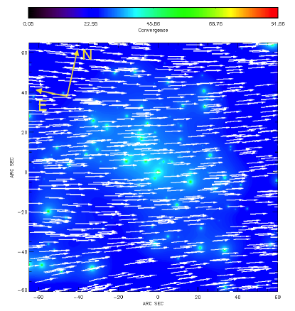
Figure 1.— False color image of the lensing convergence, $\kappa$, derived from ACS/HST strong-lensing observations centered on the bullet in the bullet cluster with the velocity field of the dark matter component of the bullet from our best fit FLASH simulation (shown in Figure 5) overlaid. The color bar on top represents the scale of the convergence. We used $S$ = 8 for the degree of the polynomial for smoothing derived from our model fitting. The image coordinates are given in arcsec as derived from observations. The center of the coordinate system is the BCG of the bullet.

3. Deflection field of the Bullet Cluster from strong lensing

In our analysis of the bullet cluster, we adopt our established method to strong-lens modeling using multiple images of background galaxies visible in the HST/Advanced Camera for Surveys (ACS) data as described in Zitrin et al. (2009). Our previous work has uncovered a large number of multiply-lensed galaxies in HST images of many clusters, including highly irregular merging systems for which the identification of multiple images had remained unsolved due to the complexity of the strong lensing regime requiring initially well-guessed models to guide the secure identification of counter images (e.g., Zitrin et al. 2011a). The basic assumption of our method is that mass approximately traces light, so that the photometry of the red cluster member galaxies is used as the starting point for the model. We identify member galaxies using HST multiband photometry based on their position in color space close to the cluster sequence. We model the mass surface density distribution of individual cluster galaxies at angular position $\theta$ assuming a symmetric power-law mass profile: $\Sigma(\mbox{\boldmath$\theta$})\propto(\mbox{\boldmath$\theta$}-\mbox{\boldmath$\theta$}_{i})^{-q}$, where $\mbox{\boldmath$\theta$}_{i}$ is the angular center of the $i$th galaxy, and $q$ is the power law index with the amplitude scaled linearly with flux. The deflection angle due to the galaxy component is the sum of all individual galaxies, which in our case can be expressed as

$$\mbox{\boldmath$\alpha$}_{\rm gal}(\mbox{\boldmath$\theta$})=A(q)\sum_{i}F_{i}\,|\mbox{\boldmath$\theta$}-\mbox{\boldmath$\theta$}_{i}|^{1-q}\,\frac{\mbox{\boldmath$\theta$}-\mbox{\boldmath$\theta$}_{i}}{|\mbox{\boldmath$\theta$}-\mbox{\boldmath$\theta$}_{i}|},$$ (11)

where the sum is over all cluster galaxies, $F_{i}$ is the flux, and the amplitude $A$ depends on $q$ and physical constants.

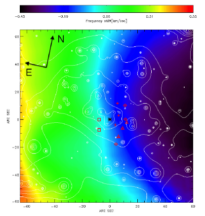
Figure 2.— Same as Figure 1, but for the frequency shift due to gravitational lensing (reconstructed from strong lensing observations) and tangential motion of the bullet (from our best fit simulation shown in Figure 5). The color bar on top represents the scale of the frequency shift in velocity units ($\rm km\,s^{-1}$). The white contours represent the convergence field shown in Figure 1 in colors. The plus signs, diamonds, triangles, and squares represent the positions of multiple lensed background galaxies (systems G, H, I, J) listed in Table 1. The star at the center marks the BCG of the bullet component.

The mass surface density distribution of the cluster DM component is approximated by smoothing the resulting mass surface density of the cluster galaxy component using a polynomial of degree $S$, which is taken as a free parameter. We derive the deflection angle of this smooth component, $\mbox{\boldmath$\alpha$}_{\rm DM}$, representing the mass distribution at each pixel with a delta function located at the pixel center:

$$\alpha_{DM}(\mbox{\boldmath$\theta$})=A(q)\sum_{i}m_{i}\,\frac{\mbox{\boldmath$\theta$}-\mbox{\boldmath$\theta$}_{i}}{(\mbox{\boldmath$\theta$}-\mbox{\boldmath$\theta$}_{i})^{2}},$$ (12)

where $m_{i}$, the mass of the $i$th cluster galaxy, represents the (unnormalized) mass value in the $i$th pixel. Since the smooth component does not perfectly follow the light, we assume an additional component for our lensing model to allow for further flexibility in the form of a coherent spin-2 external shear, $\left(\Gamma^{\rm x}\right)_{kl}$ ($k$, $l$ = 1, 2). The $k$th component of the deflection angle for this term therefore becomes: $\alpha_{{\rm x},k}(\mbox{\boldmath$\theta$})=\left(\Gamma^{\rm x}\right)_{kl}\Delta\theta_{l}$, where $\Delta\mbox{\boldmath$\theta$}$ is the displacement vector of the angular position $\theta$ with respect to a fiducial reference position. The amplitude, $|\gamma_{\,\rm x}|$, and the direction, $\phi_{\,\rm x}$, of the external shear are also free parameters in our mass model.

Our model for the deflection field, $\mbox{\boldmath$\alpha$}(\mbox{\boldmath$\theta$})$, is thus a sum of three components: the galaxy, $\mbox{\boldmath$\alpha$}_{\rm gal}(\mbox{\boldmath$\theta$})$, the smooth DM, $\mbox{\boldmath$\alpha$}_{\rm DM}(\mbox{\boldmath$\theta$})$, and a component due to the external shear, $\mbox{\boldmath$\alpha$}_{\rm x}(\mbox{\boldmath$\theta$})$, weighted as $K$, 1 - $K$, and 1 respectively:

$$\mbox{\boldmath$\alpha$}(\mbox{\boldmath$\theta$})=K\mbox{\boldmath$\alpha$}_{\rm gal}(\mbox{\boldmath$\theta$})+(1-K)\mbox{\boldmath$\alpha$}_{\rm DM}(\mbox{\boldmath$\theta$})+\mbox{\boldmath$\alpha$}_{\rm x}(\mbox{\boldmath$\theta$}),$$ (13)

where the weight, $K$, is our 5th free parameter. Including an overall normalization factor, ${\cal N}$, this model has 6 free parameters: ${\cal N},K,q,S,|\gamma_{\rm x}|,\phi_{\rm x}$. As we have demonstrated in a series of papers (Broadhurst et al., 2005; Zitrin et al., 2009, 2011a, 2011b, 2011c), this approach to strong lensing is sufficient to accurately predict the locations and internal structure of multiple images of background galaxies.

Figure 3.— Contours of convergence ($\kappa$ = 0.7,0.8,0.9,1.0) from strong lensing observations and our best fit FLASH simulation, shown in Figure 5, (blue and black contours) centered on the BCG of the bullet (North is up, East is left).

We derive our best-fit model using $\chi^{2}$ statistic, in particular, we minimize the $\chi^{2}$ derived for the image plane:

$$\chi^{2}=\displaystyle\sum_{i=1}^{n}{\frac{[\mbox{\boldmath$\theta$}_{i}-\hat{\mbox{\boldmath$\theta$}}_{i}({\cal N},K,q,S,|\gamma_{\rm x}|,\phi_{\rm x})]^{2}}{\sigma_{i}^{2}}},$$ (14)

where $i$ runs from 1 to the number of lensed images, $n$, $\mbox{\boldmath$\theta$}_{i}$ is the observed image position, $\hat{\mbox{\boldmath$\theta$}}_{i}({\cal N},K,q,S,|\gamma_{\rm x}|,\phi_{\rm x})$ is the image position given by our model, and $\sigma_{i}$ is the measurement error in the position of the $i$th lensed image. For each model parameter, we estimate the $1\,\sigma$ uncertainty by $\Delta\chi^{2}=1$ in the 6-dimensional parameter space. The uncertainties in the $\Sigma(\mbox{\boldmath$\theta$})$ field are estimated by propagating the errors of all our strong-lens model parameters.

We show in Figure 1 the convergence field of the bullet cluster derived from our strong-lensing analysis of the HST/ACS images. The smoothing was performed with a resolution of 2$\arcsec$, and the degree of the polynomial used, derived from our fitting using Equation 14, was 8. The color bar indicates the values of the convergence, $\kappa$. The large peaks of the mass density field mark the positions of individual galaxies. These peaks can be seen clearly in Figure 2 as white contours overlaid on the predicted frequency shift due to the moving cluster effect (see Section 5).

Figure 4.— Cumulative mass distribution for the two components of the bullet cluster. Squares and triangles with error bars represent masses of the main cluster and the bullet derived from lensing observations (Bradač et al., 2006), solid and dashed lines show mass profiles from our best fit FLASH simulation (Figure 5) of the main cluster and the bullet.

4. Velocity field of the Bullet Cluster from FLASH Simulations

Here we model the velocity structure of the interacting bullet cluster, using the observational features visible in this system, including the masses of the two cluster components and their separation derived from lensing, and the gross properties of the gas determined from X-ray measurements. We make use of the Eulerian adaptive mesh refinement parallel code, FLASH developed at the Center for Astrophysical Thermonuclear Flashes at the University of Chicago (Fryxell et al., 2000). We included the hydrodynamics module based on the Piecewise–Parabolic Method (PPM) of Colella & Woodward (1984), and the $N$-body module with a multigrid solver (Ricker, 2008) to represent DM particles. We adopted a box size of 13.3 Mpc on a side so that we can follow all the matter for the duration of the simulation. We reach a maximum refinement of 12.7 kpc at the high density (the cores of the mass components) and shocked regions.

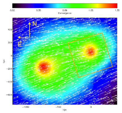
Figure 5.— False color image of the convergence with the velocity field of the bullet from our best fit FLASH simulation overlaid (white arrows). The alignment of the image is the same as that of the bullet cluster (North is up, East is left). The infalling cluster (the bullet; upper right) passed the main cluster (lower left) from the North moving toward North–West. The length of the white arrows represent the magnitude of velocity field with a maximum of about 4000 $\rm km\,s^{-1}$. The orange box represents the area of the ACS/HST strong-lensing observations shown in Figure 1.

We initially assume spherical cluster models with a cut off of the distribution of the DM and gas at the virial radius, $R_{\rm vir}$ (Bryan & Norman, 1998). Within the virial radius, we assume an NFW model (Navarro, Frenk & White, 1997) for the DM density,

$$\rho_{DM}(r)={\rho_{s}\over x(1+x)^{2}},$$ (15)

where $x=r/r_{s}$, $\rho_{s}$ and $r_{s}=r_{vir}/c_{vir}$ are scaling parameters of the density and radius, and $c_{vir}$ is the concentration parameter; and a non-isothermal $\beta$ model for the gas,

$$\rho(r)={\rho_{0}\over(1+y^{2})^{3\beta/2}},$$ (16)

where $y=r/r_{core}$, and $\rho_{0}$ and $r_{core}$ are the central density and scale radius for the intracluster gas. We derive the temperature of the gas from the equation of hydrostatic equilibrium using numerical integration. We assume an equation of state that of the ideal gas with $\gamma=5/3$. We adopt $r_{core}=0.12$ $R_{\rm vir}$, and $\beta=1$, which are consistent with our analysis of relaxed clusters of galaxies drawn from cosmological numerical simulations (see Molnar et al. 2010). Assuming a value for $M_{tot}$ and the gas mass fraction of 0.14, we derive $R_{vir}$, $\rho_{s}$, $r_{s}$, and $\rho_{0}$. We handle the small fraction of baryonic matter in galaxies along with the DM since they both may be assumed to be collisionless for our purposes. With this assumption, our DM particles also represent baryonic matter locked up in galaxies. The number of DM particles at each cell in the simulations is determined by the density and the total number of particle (we used 5 million particles). The amplitude of the velocity of each individual DM particle is derived by sampling a Maxwellian distribution (assuming a local Maxwellian approximation) with dispersion, as a function of radius, derived from the Jeans equation assuming an isotropic velocity dispersion (Łokas & Mamon, 2001). We derive the directions of the velocity vector of the DM particles assuming an isotropic distribution. For a detailed description of the setup of our FLASH simulations of merging galaxy clusters, see Molnar et al. (2012).

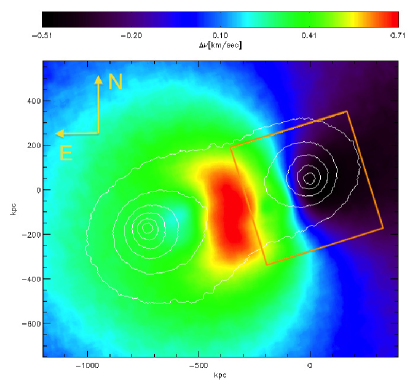
Figure 6.— Same as Figure 5, but for the frequency shift due to gravitational lensing and tangential motion of the main component and the bullet using Equation 17 with deflection angles and velocities derived from our best fit simulation. The color bar on top shows the scale of the frequency shift in velocity units ($\rm km\,s^{-1}$). The white contours depict the convergence (shown in Figure 5) using levels $\kappa$ = 0.2 to 1.2 with spacings of 0.2.

Our main goal is to determine the velocity field of the dark matter component at the central part of the the bullet using FLASH simulations which reproduce the observed main features of the mass distribution in the bullet cluster. We carry out a set of simulations with different initial masses and concentration parameters but with infall velocity and impact parameter fixed at 3000 $\rm km\,s^{-1}$ and 150 kpc, as suggested by the best model of Mastropietro & Burkert (2008). From our simulations we choose the snapshot at the same phase of the collision as observed, i.e., when the two DM centers are 800 kpc apart. From this snapshot we derive the projected mass from the profiles for both components, and compare both the mass at the center with the result from our strong lensing analysis, and compare the mass profiles with results from the lensing analysis of Bradač et al. (2006), as shown in Figure 4. We find that initial virial masses of M₁ = 9.0$\times 10^{\,14}\,$$\mbox{\rm M}_{\odot}$, M₂ = 5.5$\times 10^{\,14}\,$$\mbox{\rm M}_{\odot}$, and concentration parameters $c_{vir1}=6$, and $c_{vir2}=6$ provide a good agreement with the lensing results, although our mass profile of the bullet is shallower at the center than that from our strong lensing analysis (see Figure 3), and the mass profiles of both components are shallower than those based on lensing observations of Bradač et al. (2006), as we can see from Figure 4. Larger mass for the main component, which could provide a better fit for larger radii would yield too high a density at the center and would thus overestimate the central mass, which we avoid since we are mainly interested in the central cluster regions. Since we underestimate the masses of the two components, we also underestimate the velocity increment of the bullet due to the infall at the phase of the observation; therefore our results for the frequency changes due to the moving cluster effect should be considered as lower limits.

The best fit model of the most successful numerical simulations of the bullet cluster, the SPH simulations of Mastropietro & Burkert (2008), assumed a mass ratio of 6.25 which is much larger than ours. However, their model produces a mass profile for the main component close to ours (slightly higher), but their result for the bullet component is only a half of the observed (Figure 6 of Mastropietro & Burkert). Mastropietro & Burkert also note that, based on the mass profiles derived from lensing, the mass of the bullet seems to be a significant fraction of the total mass, and the mass ratio should be lower than even the lowest mass ratio they considered, 3:1 (and much lower than 10:1 suggested by Barrena et al. 2002; however, their result might not be very reliable because they used galaxy redshifts assuming relaxed halos and had only seven galaxies for the bullet component). Mastropietro & Burkert rejected models with lower mass ratios because in their SPH simulations the gas of the main component is disrupted to the degree that the X–ray peak of the main cluster disappears. In our AMR simulations with lower mass ratios we find that the main cluster gas is not disrupted (Molnar et al. 2013, in preparation).

Table 1Frequency shifts for multiple systems due to the moving lens effect

Name	Frequency shift in $\rm km\,s^{-1}$
	Rotation angle
	$\varphi$ = 0∘	$\varphi$ = +30∘	$\varphi$ = -30∘
G1	-0.172	0.005	-0.177
G2	-0.174	0.146	-0.253
G3	-0.130	0.290	-0.279
H1	-0.214	0.017	-0.226
H2	-0.198	0.174	-0.289
H3	-0.089	0.468	-0.316
I1	-0.122	0.395	-0.316
I2	-0.194	0.210	-0.300
I3	-0.161	0.300	-0.314
J1	0.016	0.386	-0.178
J2	0.016	0.272	-0.124

Using our simulations of the best fit mass distribution model at the phase of the bullet cluster (distance between the two DM centers equal to 120 kpc), we generate DM surface mass density maps $\Sigma(\theta)$, and velocity field maps for the two mass components. We integrate the total (DM and gas) density along the LOS assuming that the collision is in the plane of the sky (good approximation for the bullet cluster, e.g., Mastropietro & Burkert 2008) to obtain the mass surface density images and convert the density map to a convergence map using the physical parameters relevant to the bullet cluster. We determine the average velocity at each position using the median of all bulk-velocity motions along the LOS. We show the color image of the convergence for this phase of the collision in Figure 5. The alignment of the image in RA and DEC is the same as that of the bullet cluster. The image coordinates are given in physical units (kpc) centered on the peak in the surface mass density corresponding to the bullet. In this simulated image, the bullet, moving from left to right, just passed the core of the main cluster (first core passage) from the North. The white arrows represent the bulk motion of the mass within the cluster. The length of the arrows show the amplitude of the velocities (with a maximum of 4000 $\rm km\,s^{-1}$). Dominated by the bulk flow of the DM component of the bullet, we find that the velocity field is smooth in the vicinity of the bullet DM center (Figure 1), as we expected.

5. Results and Discussion

Here we first derive the expected frequency shifts due to the moving cluster effect using the velocity and deflection fields determined from our simulations of the bullet cluster. In our case, Equation 5 reduces to the sum of the two components, and the frequency shift field from simulations, expressed in velocity units, can be calculated as

$$V^{sim}(x,y)=\mbox{\boldmath$v$}_{T1}\cdot\mbox{\boldmath$\alpha$}_{1}+\mbox{\boldmath$v$}_{T2}\cdot\mbox{\boldmath$\alpha$}_{2},$$ (17)

where the 2D vector fields $\mbox{\boldmath$v$}_{T1,2}$ and $\mbox{\boldmath$\alpha$}_{1,2}$ represent the tangential velocities and the deflection angle of the main cluster (1) and the bullet (2). The frequency shift field expected over the surface of the cluster are shown in Figure 6. A dipole pattern for the fast–moving component, the bullet, can be clearly seen on the right hand side of the image. The difference between the maximum and minimum frequency shift due to the tangential motion of the bullet is 1.2 $\rm km\,s^{-1}$.

Table 2Large frequency shift differences due to the moving cluster effect

Name	Frequency shift difference in $\rm km\,s^{-1}$
	Moving lens effect			Moving observer
	$\varphi$ = 0∘	$\varphi$ = +30∘	$\varphi$ = -30∘	no $\varphi$ dependence
G3-G1	-	0.284	0.103	-0.020
G3-G2	-	-	-	-
G2-G1	-	-	-	-0.009
H3-H1	0.125	0.451	-	-0.035
H3-H2	0.109	-	-	-0.024
I2-I1	-	0.185	-
J2-J1	-	0.115	-

Our simulations do not include structures smaller than the two primary mass components, approximating the bullet cluster system. We also ignore the often significant contribution of member galaxies to the lensing deflection field in our idealized simulations. So here we make the frequency shift calculation more realistic by deriving the lensing deflection field using the actual observed multiple images with our lens model for which the observed member galaxies are incorporated (see Section 3). Details of the velocity field are not that important as this field is inherently smooth, being dominated by the bulk motions of the DM components of the two main clusters, and therefore this field is reasonably well mapped, as shown above. In the vicinity of the bullet the observed deflection field is mainly due to the DM component of the bullet, and both the velocity of the DM and the deflection field generated by the main cluster are negligible. In this case, Equation 5 reduces to Equation 3, and we can approximate the expected frequency shift due to the moving cluster effect as

$$V(x,y)=\mbox{\boldmath$v$}_{T}(x,y)\cdot\mbox{\boldmath$\alpha$}(x,y),$$ (18)

where the velocity field of the bullet, $\mbox{\boldmath$v$}_{T}(x,y)$ is taken from our FLASH simulations (Section 4) and the deflection field, $\mbox{\boldmath$\alpha$}(x,y)$, is from our strong lensing analysis (Section 3). In Figure 1 we show the velocity field from our simulations (white arrows) oriented to match the alignment of the ACS/HST images of the bullet cluster plotted over the convergence field we derive from strong lensing. The map of the frequency shifts is plotted in units of $\rm km\,s^{-1}$ in Figure 2 (with white contours overlaid representing the convergence field shown in Figure 1 in colors).

From the frequency shift field, $V(x,y)$, shown in Figure 2 we now evaluate the expected frequency shifts at the positions of the multiply-imaged background galaxies, $V_{i}=V(\mbox{\boldmath$\theta$}_{I}^{i}$), as identified by Bradač et al. (2006). We show the list of the frequency shifts due to the moving cluster effect in velocity units in Table 1. The first column is the ID designation of the system as in Bradac et al. The second column represents the frequency shifts we obtain when we align the velocity field derived from simulations with the deflection angle from strong lensing observations. The remaining 2 columns illustrate possible systematic errors in the frequency shifts allowing $\pm 30$^∘ rotation angles, $\varphi$, relative to the rotation angle chosen for the alignment of simulations and observations.

In principle, we can measure the relative frequency shift between any of the counter images belonging to each multiply-lensed background galaxy. These relative frequency shifts are shown in Table 2 for systems that we expect to exceed 0.100 $\rm km\,s^{-1}$. From this table we find that two triply–imaged systems (G and H) having the largest relative frequency shifts about 0.5 $\rm km\,s^{-1}$  depending on the orientation of the DM velocity field. However, we consider these as underestimated relative shifts, since we find that at this infall velocity (3000 $\rm km\,s^{-1}$), our preliminary AMR simulations, aimed to explain the mass surface distribution, and the X–ray and SZ morphology, have insufficient Ram pressure to reproduce the observed displacement between the DM center of the lower mass bullet component and the bullet gas. Instead we find that an initial relative velocity of 4500 $\rm km\,s^{-1}$ is required between the cluster components in order to create a distinct bullet with a sizable offset between the gas and dark mater, as observed. This larger impact velocity would result in frequency shifts of about 50% larger than those based on an impact velocity of 3000 $\rm km\,s^{-1}$ we are using in our analysis. As a result, our estimates for the frequency shifts due to tangential motion of the bullet cluster can be considered as conservative lower estimates.

As a consistency check we estimate the relative frequency shifts due to the tangential motion of the observer, $\mbox{\boldmath$v$}_{T}^{\,O}$. In the case of the bullet cluster, the relative frequency shift for the $i$th lensed image, at the image position, $\mbox{\boldmath$\theta$}_{I}^{i}$, expressed in velocity units using the second term in Equation 5, becomes

$$V_{{\rm X}i}=-\frac{D_{LS}(z,z_{\rm X})}{D_{OS}(z_{\rm X})}\,\mbox{\boldmath$v$}_{T}^{\,O}\cdot\mbox{\boldmath$\alpha$}(\mbox{\boldmath$\theta$}_{I}^{i}),$$ (19)

where X is the index for the lensed background galaxy, X = G, H, I, or J, and $z_{\rm X}$ is the corresponding redshift, $z_{\rm G}$ = 1.3, $z_{\rm H}$ = 1.9, $z_{\rm I}$ = 2.1, $z_{\rm J}$ = 1.7 (Bradač et al., 2006). We obtain $\mbox{\boldmath$v$}_{T}^{\,O}$ by projecting our Heliocentric velocity relative to the CMB, $\mbox{\boldmath$v$}^{\,O}$, to the plane of the sky of the bullet cluster. Using RA = 6h 58m 37.9s; DEC = -55^∘ 57′ 0″ for the position of the bullet cluster and $v^{\,O}$ = 369.0 $\rm km\,s^{-1}$ pointing toward RA = 11h 11m 43s; DEC = -6^∘ 55′ 37″ for the velocity of the observer (Hinshaw et al., 2009), we obtain $v_{T}$ = 345.672 $\rm km\,s^{-1}$, with a rotation angle of 103.^∘9 relative to the velocity of the bullet in the plane of the sky. We find that the largest relative frequency shift due to the observer’s motion is 35 $\rm m\,s^{-1}$ (for the H3-H1 pair), and in most cases, these frequency shifts are around 20 $\rm m\,s^{-1}$, thus we conclude that these can be safely neglected (see Table 2).

As we have shown above such predicted frequency shifts are within the range of the ALMA array for molecular CO(1–0) emission and near the resolution limit in the optical-IR using X-shooter on the VLT. Ideally the velocity resolution should be sufficient to allow for the definition of a detailed velocity profile over the emission lines detected for each component of a given multiply-lensed galaxy, so that repeatable velocity substructure can be identified and used to help establish the small relative velocity shifts induced by the tangential motion of the lens. There is a great advantage in using systems with more than 2 multiple images in that the direction of the motion of the cluster mass can be solved for (see our Equation 9) without the need for models of the DM motion.

6. Final Comments

High speed motions recently inferred from large scale shocked gas and offsets between the positions of DM and gas in colliding clusters seem surprising in the context of standard cosmological models. The bullet cluster, which provided the first example for this phenomenon, is claimed to be in grave conflict with the concordance $\Lambda$CDM model, where no such high speed encounters of such massive clusters is predicted in even the largest simulations. However, as we discussed in the introduction, several other merging clusters exist with inferred large relative impact velocities.

The main motivation for considering the challenging observations proposed here lies in the ability to measure the motion of dark matter directly from observed frequency shifts due to the moving cluster effect. The moving cluster effect investigated here is generated by the motion of the gravitational potential and therefore its importance lies in the direct relation to the motion of the dominant DM, unlike the kSZ effect, for which gas modeling is required. The bulk motion of the DM is smooth even in merging clusters, as we demonstrated using our simulations, therefore it is much easier to model this motion unlike that of the gas which has a complicated velocity field due to non-gravitational interactions.

We have examined the moving cluster effect on the relative frequency shifts between multiply-imaged background galaxies in the bullet cluster from detailed modeling of the velocity and gravitational potential fields. Our results are shown in Table 2. We have found two triply-imaged systems having the largest relative frequency shift of about 0.5 $\rm km\,s^{-1}$ depending on the orientation of the dark-matter velocity field. We have found that at this infall velocity, our AMR simulation has insufficient Ram pressure to reproduce the observed displacement between the dark-matter center of the bullet component and the bullet gas, which we find requires initial relative velocities of as large as 4500 $\rm km\,s^{-1}$ for which a distinct bullet is created with a relatively large offset between the gas and DM, as observed. This larger impact velocity would result in frequency shifts of about 50% larger than those based on the impact velocity of 3000 $\rm km\,s^{-1}$ we assumed in our analysis. As a result, our estimates for the frequency shifts due to tangential motion of the bullet cluster are conservative. These predicted frequency shifts are within the range of the ALMA array for molecular CO(1–0) emission and near the resolution limit in the optical-IR using X-shooter on the VLT.

This proposed method can be extended to smaller frequency shifts using many independent lines of the Lyman-$\alpha$ forest towards distant QSOs lensed by more typical clusters of galaxies, complementary to line-of-sight peculiar motions derived from the kinematic SZ effect, so that the 3D peculiar motions of individual clusters may be reconstructed from direct measurements.

References

- AMI Consortium et al. (2011) AMI Consortium, Rodríguez-Gonzálvez, C., Olamaie, M., et al. 2011, MNRAS, 414, 3751
- Barcons, X., et al. (2012) Barcons, X., et al., 2012, preprint, arXiv:1102.2845
- Barrena et al. (2002) Barrena, R., Biviano, A., Ramella, M., Falco, E. E., & Seitz, S. 2002, A&A, 386, 816
- Birkinshaw (1999) Birkinshaw, M. 1999, Phys. Rep., 310, 97
- Birkinshaw & Gull (1983) Birkinshaw, M., & Gull, S. F. 1983, Nature, 302, 315
- Bradač et al. (2006) Bradač M., Clowe D., Gonzalez A. H., Marshall P., Forman W., Jones C., Markevitch M., Randall S., et al., 2006, ApJ, 652, 937
- Broadhurst & Scannapieco (2000) Broadhurst, T., & Scannapieco, E. 2000, ApJ, 533, L93
- Broadhurst et al. (2005) Broadhurst, T., Benítez, N., Coe, D., et al. 2005, ApJ, 621, 53
- Bryan & Norman (1998) Bryan, G. L., & Norman, M. L. 1998, ApJ, 495, 80
- Cai et al. (2010) Cai, Y.-C., Cole, S., Jenkins, A., & Frenk, C. S. 2010, MNRAS, 407, 201
- Carlstrom et al. (2002) Carlstrom, J. E., Holder, G. P., & Reese, E. D. 2002, ARA&A, 40, 643
- Christensen et al. (2010) Christensen, L., D’Odorico, S., Pettini, M., et al. 2010, MNRAS, 406, 2616
- Clowe et al. (2004) Clowe D., Gonzalez A., & Markevitch M., 2004, ApJ, 604, 596
- (14) Clowe D., Bradač M., Gonzalez A. H., Markevitch M., Randall S. W., Jones C., & Zaritsky D., 2006, ApJ, 648, L109
- Colella & Woodward (1984) Colella, P., & Woodward, P. R. 1984, Journal of Computational Physics, 54, 174
- Crocce et al. (2010) Crocce, M., Fosalba, P., Castander, F. J., & Gaztañaga, E. 2010, MNRAS, 403, 1353
- Dahle et al. (2012) Dahle, H., Gladders, M. D., Sharon, K., et al. 2012, arXiv:1211.1091
- Dawson et al. (2012) Dawson, W. A., Wittman, D., Jee, M. J., et al. 2012, ApJ, 747, L42
- Fohlmeister et al. (2007) Fohlmeister, J., Kochanek, C. S., Falco, E. E., et al. 2007, ApJ, 662, 62
- Fohlmeister et al. (2013) Fohlmeister, J., Kochanek, C. S., Falco, E. E., et al. 2013, ApJ, 764, 186
- Farrar & Rosen (2007) Farrar, G. R., & Rosen, R. A. 2007, Physical Review Letters, 98, 171302
- Fryxell et al. (2000) Fryxell, B., et al. 2000, ApJS, 131, 273
- Gurvits & Mitrofanov (1986) Gurvits, L. I., & Mitrofanov, I. G., 1983, 324, 349
- Hand et al. (2012) Hand, N., Addison, G. E., Aubourg, E., et al. 2012, Physical Review Letters, 109, 041101
- Harko (2011) Harko, T. 2011, Phys. Rev. D, 83, 123515
- Hayashi & White (2006) Hayashi E., White S. D. M., 2006, MNRAS, 370, L38
- Hinshaw et al. (2009) Hinshaw, G., Weiland, J. L., Hill, R. S., et al. 2009, ApJS, 180, 225
- Host (2012) Host, O. 2012, MNRAS, 420, L18
- Inada et al. (2006) Inada, N., Oguri, M., Morokuma, T., et al. 2006, ApJ, 653, L97
- Inada et al. (2003) Inada, N., Oguri, M., Pindor, B., et al. 2003, Nature, 426, 810
- Kain & Ling (2012) Kain, B., & Ling, H. Y. 2012, Phys. Rev. D, 85, 023527
- Killedar & Lewis (2010) Killedar, M., & Lewis, G. F. 2010, MNRAS, 402, 650
- Korngut et al. (2011) Korngut, P. M., Dicker, S. R., Reese, E. D., et al. 2011, ApJ, 734, 10
- Lee & Komatsu (2010) Lee, J., & Komatsu, E. 2010, ApJ, 718, 60
- Łokas & Mamon (2001) Łokas, E. L., & Mamon, G. A. 2001, MNRAS, 321, 155
- Madarassy & Toth (2002) Madarassy, E. J. M., & Toth, V. T., 2012, arXiv:1207.5249
- Mak, Pierpaoli & Osborne (2011) Mak, D. S. Y., Pierpaoli, E., & Osborne, S. J. 2011, ApJ, 736, 116
- Markevitch et al. (2004) Markevitch, M., Gonzalez, A. H., Clowe, D., et al. 2004, ApJ, 606, 819
- Markevitch (2005) Markevitch, M., 2005, preprint, astro-ph/0511345
- Mastropietro & Burkert (2008) Mastropietro, C., & Burkert, A. 2008, MNRAS, 389, 967
- Maturi et al. (2007) Maturi, M., Enßlin, T., Hernández-Monteagudo, C., & Rubiño-Martín, J. A. 2007, A&A, 467, 411
- Menanteau et al. (2012) Menanteau, F., Hughes, J. P., Sifón, C., et al. 2012, ApJ, 748, 7
- Merten et al. (2011) Merten, J., Coe, D., Dupke, R., et al. 2011, MNRAS, 417, 333
- Milosavljević et al. (2007) Milosavljević, M., Koda, J., Nagai, D., Nakar, E., & Shapiro, P. R. 2007, ApJ, 661, L131
- Molnar & Birkinshaw (2003) Molnar, S. M., & Birkinshaw, M. 2003, ApJ, 586, 731
- Molnar et al. (2012) Molnar, S. M., Hearn, N. C., & Stadel, J. G. 2012, ApJ, 748, 45
- Molnar et al. (2010) Molnar, S. M., et al. 2010, ApJ, 723, 1272
- Mroczkowski et al. (2012) Mroczkowski, T., Dicker, S., Sayers, J., et al. 2012, ApJ, 761, 47
- Navarro, Frenk & White (1997) Navarro, J. F., Frenk, C. S., & White, S. D. M. 1997, ApJ, 490, 493
- Ota et al. (2012) Ota, N., Oguri, M., Dai, X., et al. 2012, ApJ, 758, 26
- Peacock et al. (2001) Peacock, J. A., Cole, S., Norberg, P., et al. 2001, Nature, 410, 169
- Planck Collaboration: Ade et al. (2001) Planck Collaboration: Ade et al. 2013, arXiv:1303.5077v1
- Pyne & Birkinshaw (1993) Pyne, T., Birkinshaw, M., 1993, ApJ, 415, 459
- Raychaudhury & Saslaw (1996) Raychaudhury, S., & Saslaw,W. C. 1996, ApJ, 564, 514
- Reid et al. (2012) Reid, B. A., Samushia, L., White, M., et al. 2012, MNRAS, 426, 2719
- Ricker (2008) Ricker, P. M. 2008, ApJS, 176, 293