On the filtering effect of iterative regularization algorithms for linear least-squares problems

Abstract

Many real-world applications are addressed through a linear least-squares problem formulation, whose solution is calculated by means of an iterative approach. A huge amount of studies has been carried out in the optimization field to provide the fastest methods for the reconstruction of the solution, involving choices of adaptive parameters and scaling matrices. However, in presence of an ill-conditioned model and real data, the need of a regularized solution instead of the least-squares one changed the point of view in favour of iterative algorithms able to combine a fast execution with a stable behaviour with respect to the restoration error. In this paper we want to analyze some classical and recent gradient approaches for the linear least-squares problem by looking at their way of filtering the singular values, showing in particular the effects of scaling matrices and non-negative constraints in recovering the correct filters of the solution.

1 Introduction

We consider the classical linear least-squares problem

$$\min_{\boldsymbol{x}\in\mathbb{R}^{n}}f(\boldsymbol{x})\equiv\frac{1}{2}\|\boldsymbol{A}\boldsymbol{x}-\boldsymbol{b}\|_{2}^{2},$$ (1)

where $\boldsymbol{A}$ is a full-rank $m\times n$ matrix, with $m\geq n$, and $\boldsymbol{b}\in\mathbb{R}^{m}$. Such issue is typically addressed in presence of an ill-posed inverse problem

$$\boldsymbol{A}\boldsymbol{x}=\boldsymbol{b},$$ (2)

since the existence and uniqueness of the least-squares solution $\boldsymbol{x}^{\dagger}$ together with its continuously data dependence (that is guaranteed in the discrete case) lead to a well-posed problem. However, especially in the case in which the linear system (2) arises from the discretization of a continuous ill-posed inverse problem, the switch to the least-squares problem (1) does not avoid the ill-conditioning pathology, that amplifies the noise affecting the data with the result of a meaningless reconstructed solution. A classical example occurs in the image deblurring problem [4, 19], in which $\boldsymbol{b}$ is a blurred and noisy version of an unknown image $\boldsymbol{x}$ and $\boldsymbol{A}$ describes the transformation from the target to the measured data values. The numerical instability provided by the ill-conditioning can be countered by looking for a regularized solution of (1), obtained by means of an approximation of the original problem with a one-parameter family of better conditioned ones. A strategy for the choice of the “best” parameter is finally needed, according to some criteria based for example on the knowledge of the noise level or the analysis of the residuals [14, 18, 26]. Besides the classical direct regularization approaches as the truncated singular value decomposition or the Tikhonov method, an increasing interest has been devoted to iterative regularization strategies, that are in general more computationally effective for large scale problems and allow an easier introduction of constraints on the desired solution (e.g., non-negativity, flux conservation) [2, 3, 4, 5, 26]. Although in general the regularization property of iterative approaches is not theoretically proved, most of them exhibits the so-called semiconvergence effect, i.e., the reconstruction error decreases until one optimal iterate and then diverges. Such behaviour has been analyzed e.g. by Nagy & Palmer [22] and Donatelli & Serra Capizzano [13] in terms of filter factors [19]. In particular, in [22] some classical gradient methods have been reformulated as a linear combination of the singular vectors of $\boldsymbol{A}$, in which the coefficients form involves the inverse of the singular values $\sigma_{i}$ multiplied for suitable factors that balance possible noise amplification effects due to small values of some $\sigma_{i}$. In this paper we want to go one step further, proving that a similar expansion holds true even if a scaling matrix multiplying the gradient is present. Moreover, we investigate the effect on the filter factors of some scaling matrices, arising from both the numerical optimization and the imaging framework. In particular, we show that the apparently negative oscillating behaviour of the filters provided by some scaled schemes results to be a surplus value for a more detailed reconstruction of the true solution. Finally, we extend our analysis to a particular class of projected gradient methods in the case of non-negative solutions.
The plan of the paper is the following: in Section 2 we introduce the optimization methods for the solution of (1) we decided to analyze, while in Section 3 the state-of-the-art on such algorithms as filtering methods is summarized, and the extensions to the scaled and projected cases are provided. Section 4 shows the behaviour of the filter factors for the considered regularization algorithms through some numerical experiments, while our conclusions are offered in Section 5.

2 Gradient methods

A gradient method for the solution of (1) is an iterative algorithm whose $(k+1)$–th element is defined by

$$\boldsymbol{x}_{k+1}=\boldsymbol{x}_{k}-\alpha_{k}\boldsymbol{M}_{k}\boldsymbol{g}_{k},$$ (3)

where:

• $\boldsymbol{g}_{k}=\nabla f(\boldsymbol{x}_{k})=\boldsymbol{A}^{T}(\boldsymbol{A}\boldsymbol{x}_{k}-\boldsymbol{b})$ is the gradient vector;

• $\boldsymbol{M}_{k}$ is a symmetric and positive definite scaling matrix;

• $\alpha_{k}$ is the steplength parameter.

In the literature, a large variety of possibilities for choosing the steplength $\alpha_{k}$ and the scaling matrix $\boldsymbol{M}_{k}$ has been proposed. Classical examples of steplength selection are the Steepest Descent (SD) [9] and the Minimal Gradient (MG) [10, 27] methods, which minimize $f(\boldsymbol{x}_{k}-\alpha\boldsymbol{M}_{k}\boldsymbol{g}_{k})$ and $\|\nabla f(\boldsymbol{x}_{k}-\alpha\boldsymbol{M}_{k}\boldsymbol{g}_{k})\|_{2}$, respectively:

$$\alpha_{k}^{SD}=\underset{\alpha\in\mathbb{R}}{\text{argmin}}\ f(\boldsymbol{x}_{k}-\alpha\boldsymbol{M}_{k}\boldsymbol{g}_{k})=\frac{\boldsymbol{g}_{k}^{T}\boldsymbol{M}_{k}\boldsymbol{g}_{k}}{\|\boldsymbol{A}\boldsymbol{M}_{k}\boldsymbol{g}_{k}\|_{2}^{2}}.$$ (4)

$$\alpha_{k}^{MG}=\underset{\alpha\in\mathbb{R}}{\text{argmin}}\ \|\nabla f(\boldsymbol{x}_{k}-\alpha\boldsymbol{M}_{k}\boldsymbol{g}_{k})\|_{2}=\frac{\boldsymbol{g}_{k}^{T}\boldsymbol{M}_{k}\boldsymbol{A}^{T}\boldsymbol{A}\boldsymbol{g}_{k}}{\|\boldsymbol{A}^{T}\boldsymbol{A}\boldsymbol{M}_{k}\boldsymbol{g}_{k}\|_{2}^{2}}.$$ (5)

In order to accelerate the slow convergence exhibited in most cases by the standard formulas (4) and (5), many other strategies for the steplength selection have been proposed, as the two Barzilai and Borwein (BB) rules [1]

$$\alpha_{k}^{BB1}=\frac{\boldsymbol{s}_{k-1}^{T}\boldsymbol{s}_{k-1}}{\boldsymbol{s}_{k-1}^{T}\boldsymbol{y}_{k-1}}\qquad;\qquad\alpha_{k}^{BB2}=\frac{\boldsymbol{s}_{k-1}^{T}\boldsymbol{y}_{k-1}}{\boldsymbol{y}_{k-1}^{T}\boldsymbol{y}_{k-1}},$$

where $\boldsymbol{s}_{k-1}=\boldsymbol{x}_{k}-\boldsymbol{x}_{k-1}$ and $\boldsymbol{y}_{k-1}=\boldsymbol{g}_{k}-\boldsymbol{g}_{k-1}$. These two schemes have been adapted to account for the scaling matrix [7] as follows

$$\alpha_{k}^{BB1S}=\frac{\boldsymbol{s}_{k-1}^{T}\boldsymbol{M}_{k}^{-1}\boldsymbol{M}_{k}^{-1}\boldsymbol{s}_{k-1}}{\boldsymbol{s}_{k-1}^{T}\boldsymbol{M}_{k}^{-1}\boldsymbol{y}_{k-1}}\qquad;\qquad\alpha_{k}^{BB2S}=\frac{\boldsymbol{s}_{k-1}^{T}\boldsymbol{M}_{k}\boldsymbol{y}_{k-1}}{\boldsymbol{y}_{k-1}^{T}\boldsymbol{M}_{k}\boldsymbol{M}_{k}\boldsymbol{y}_{k-1}}.$$

Further accelerations have been proposed hereafter by alternating different steplength rules by means of an adaptively controlled switching criterion. Examples of such rules are the Adaptive Steepest Descent (ASD) method, the Adaptive Barzilai-Borwein (ABB) method [27] and its generalizations $\text{ABB}_{\text{min1}}$ and $\text{ABB}_{\text{min2}}$ provided by Frassoldati et al. [15].
As far as the scaling matrix concerns, the first example we considered is given by the well-known conjugate gradient algorithm for the least squares problem (CGLS). Indeed, this method can be expressed in the form (3) by choosing the SD steplength and the scaling matrix

$$\boldsymbol{M}_{k}=\boldsymbol{I}-\frac{\boldsymbol{s}_{k-1}\boldsymbol{y}_{k-1}^{T}}{\boldsymbol{y}_{k-1}^{T}\boldsymbol{s}_{k-1}}.$$

In our analysis, we also included two scaling matrices arising from the constrained optimization case. The first is the one provided by the iterative space reconstruction algorithm (ISRA), proposed by Daube-Whiterspoon and Muehllener [12] for reducing the computational cost of the expectation-maximization (EM) algorithm of Shepp and Vardi [25] in emission tomography. The explicit expression of the scaling matrix is

$$\boldsymbol{M}_{k}=\text{diag}\left(\frac{\boldsymbol{x}_{k}}{\boldsymbol{A}^{T}\boldsymbol{A}\boldsymbol{x}_{k}}\right),$$

where the quotient is intended in the Hadamard sense, and we obtain the positive definiteness by thresholding the diagonal elements in a prefixed interval $0<L_{\min}<L_{\max}$.
The second scaling matrix is the one described in [16] by Hager, Mair and Zhang (HMZ), that exploits a gradient splitting strategy [20, 21] with a resulting scaling matrix given by

$$\boldsymbol{M}_{k}=\text{diag}\left(\frac{\alpha_{k}^{CBB1}\boldsymbol{x}_{k}}{\boldsymbol{x}_{k}+\alpha_{k}^{CBB1}(\boldsymbol{A}^{T}\boldsymbol{A}\boldsymbol{x}_{k}-\boldsymbol{A}^{T}\boldsymbol{b})^{+}}\right),$$ (6)

where $t^{+}=\max\{0,t\}$ and $\alpha_{k}^{CBB1}$ is a cyclic version of the first BB steplength rule computed by reusing $\alpha_{k}^{BB1}$ for $p$ consecutive iterations [11]. A further thresholding step assures again the positive definiteness of the scaling matrix.
We remark that here we are not considering the ISRA and HMZ algorithms, but we only borrow the scaling matrices defined in the algorithms themselves and use them in our scaled gradient scheme.
We point out that, while the convergence of the nonscaled gradient methods with the steplengths described before is guaranteed, the presence of a scaling matrix might require a thresholding of the steplength in a fixed range of positive values $[\alpha_{min},\alpha_{max}]$, followed by the introduction of a successive steplength reduction strategy. A classical example is the well-known Armijo rule [6]: for given scalars $0<\gamma,\beta<1$ and $z_{k}>0$, the steplength $\alpha_{k}$ is set equal to $\beta^{q_{k}}z_{k}$, where $q_{k}$ is the first non-negative integer $q$ for which

$$f(\boldsymbol{x}_{k})-f(\boldsymbol{x}_{k}-\beta^{q}z_{k}\boldsymbol{M}_{k}\nabla f(\boldsymbol{x}_{k}))\geq\gamma\beta^{q}z_{k}\nabla f(\boldsymbol{x}_{k})^{T}\boldsymbol{M}_{k}\nabla f(\boldsymbol{x}_{k}).$$

3 Filtering effect

When considering a linear inverse problem with noisy data

$$\boldsymbol{b}=\boldsymbol{A}\boldsymbol{x}_{\text{true}}+\boldsymbol{\eta},$$

it is well-known that the role played by a regularization method is to contrast the amplifying effect on the noise $\boldsymbol{\eta}$ due to the small singular values of $\boldsymbol{A}$. Indeed, if $\boldsymbol{A}=\boldsymbol{U}\boldsymbol{\Sigma}\boldsymbol{V}^{T}$ is the singular value decomposition of the matrix $\boldsymbol{A}$, $\boldsymbol{u}_{i}$, $\boldsymbol{v}_{i}$ are the columns of $\boldsymbol{U}$, $\boldsymbol{V}$ and $\sigma_{1}\geq\ldots\geq\sigma_{n}>0$ are the diagonal elements of $\boldsymbol{\Sigma}$, then the following relation for the solution $\boldsymbol{x}^{\dagger}$ of (1) holds:

$$\boldsymbol{x}^{\dagger}=\sum_{i=1}^{n}\frac{\boldsymbol{u}_{i}^{T}\boldsymbol{b}}{\sigma_{i}}\boldsymbol{v}_{i}=\boldsymbol{x}_{\text{true}}+\sum_{i=1}^{n}\frac{\boldsymbol{u}_{i}^{T}\boldsymbol{\eta}}{\sigma_{i}}\boldsymbol{v}_{i}.$$ (7)

The classical recipe to contain the error propagation on the regularized solution $\boldsymbol{x}_{\text{reg}}$ consists of adding some weights in the linear combination (7) that filter out the last components:

$$\boldsymbol{x}_{\text{reg}}=\sum_{i=1}^{n}\phi_{i}\frac{\boldsymbol{u}_{i}^{T}\boldsymbol{b}}{\sigma_{i}}\boldsymbol{v}_{i}.$$ (8)

The truncated singular value decomposition (TSVD) and the Tikhonov method are examples of this approach, and the corresponding regularized solutions can be written in the form (8) with, respectively,

$$\phi_{i}=\begin{cases}1&\text{if }\ i\leq r\\ 0&\text{if }\ i>r\end{cases}\qquad;\qquad\phi_{i}=\frac{\sigma_{i}^{2}}{\sigma_{i}^{2}+\lambda},$$

where $r\in\{1,\ldots,n\}$ and $\lambda>0$.

3.1 The nonscaled case

Besides the classical “direct” approaches as TSVD and Tikhonov, also iterative regularization strategies can be thought by means of their filtering effect. Indeed, expression (8) can be generalized to the regularized solution $\boldsymbol{x}_{k+1}$ provided by any gradient method by writing

$$\boldsymbol{x}_{k+1}=\sum_{i=1}^{n}\phi_{i}^{k+1}\frac{\boldsymbol{u}_{i}^{T}\boldsymbol{b}}{\sigma_{i}}\boldsymbol{v}_{i}.$$

where the filter factors $\phi_{i}^{k+1}$ are automatically defined during the iterative procedure. The easiest example of gradient method is the Landweber algorithm, which generates a sequence $\{\boldsymbol{x}_{k}\}$ by

$$\boldsymbol{x}_{k+1}=\boldsymbol{x}_{k}-\alpha\boldsymbol{g}_{k}=\boldsymbol{x}_{k}-\alpha\boldsymbol{A}^{T}(\boldsymbol{A}\boldsymbol{x}_{k}-\boldsymbol{b})\,,$$ (9)

where the steplength $\alpha$ is fixed during the iterations and must satisfy $0<\alpha<2/\sigma_{1}^{2}$ in order to guarantee the convergence. The iteration (9) can be rewritten, by choosing the initial guess $\boldsymbol{x}_{0}=\boldsymbol{0}$, as

$$\boldsymbol{x}_{k+1}=\alpha\sum_{\ell=0}^{k}(\boldsymbol{I}-\alpha\boldsymbol{A}^{T}\boldsymbol{A})^{\ell}\boldsymbol{A}^{T}\boldsymbol{b}$$

or, equivalently, by means of the SVD as

$$\boldsymbol{x}_{k+1}=\sum_{i=1}^{n}\left(1-(1-\alpha\sigma_{i}^{2})^{k+1}\right)\frac{\boldsymbol{u}_{i}^{T}\boldsymbol{b}}{\sigma_{i}}\boldsymbol{v}_{i}\,,$$

thus obtaining an expression for the filter factors given by

$$\phi_{i}^{k+1}=1-(1-\alpha\sigma_{i}^{2})^{k+1}\quad k=0,1,\ldots$$

The previous equation suggests an extension to the case of the steplength $\alpha_{k}$ varying at each iteration, in the case of nonscaled gradient. If $\boldsymbol{M}_{k}=\boldsymbol{I}$, indeed, the filter factors of a general gradient method can be written as

$$\phi_{i}^{k+1}=1-\prod_{\ell=0}^{k}\bigl{(}1-\alpha_{\ell}\sigma_{i}^{2}\bigr{)}\quad k=0,1,\ldots$$ (10)

Since the sequence generated by the gradient method converges to the least-squares solution $\boldsymbol{x}^{\dagger}$, the filter factors $\phi_{i}^{k+1}$ will tend to 1 as $k$ increases. Moreover, from the form of the products in (10) we can observe that the convergence rate of the sequence $\{\phi_{i}^{k+1}\}$ to its limit value depends on the steplength values $\alpha_{\ell}$. In Figure 1, the filter factors obtained in a numerical experiment with different steplength rules have been reported as functions of the singular values index $i$. In particular, we considered the heat dataset from Hansen’s Regularization Tools [17] and we plotted the filter factors generated at iteration 10, 30 and at the iteration corresponding to the minimum error for gradient methods with the MG, SD, BB1, BB2, ABB and ABB${}_{\text{min1}}$ steplength rules (in this very last case, we used the revised version of the ABB${}_{\text{min1}}$ scheme proposed in [24]). In all cases the filter factors start from zero (since we chose $\boldsymbol{x}_{0}=\boldsymbol{0}$ as initial point) and converge to 1, with a faster convergence clearly visible for the factors corresponding to the largest singular values. Moreover, the regular and smooth filter trends achieved in all the figures show that any steplength selection rule is not able to generate filter factors that behave as erratically as the true ones given by $\sigma_{i}(\boldsymbol{v}_{i}^{T}\boldsymbol{x}_{\text{true}})/(\boldsymbol{u}_{i}^{T}\boldsymbol{b})$.

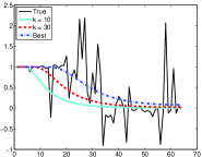
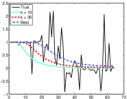
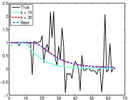
MG	SD	BB1
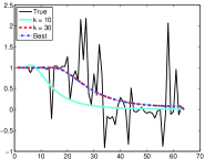
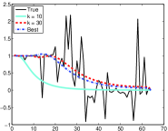
BB2	ABB	ABB${}_{\text{min1}}$

Figure 1: Comparison of the $\boldsymbol{x}_{\text{true}}$ filter factors (black thin) for the heat test problem with the ones generated by gradient methods with different steplength rules at iteration 10 (cyan thick), 30 (red dashed) and at the iteration corresponding to the minimum error (blue dashdot).

3.2 Adding a scaling matrix

If we assume $\boldsymbol{x}_{0}=\boldsymbol{0}$, then the general expression (3) of a gradient method can be easily rewritten in the form

$$\boldsymbol{x}_{k+1}=P_{k}(\boldsymbol{A}^{T}\boldsymbol{A})\boldsymbol{A}^{T}\boldsymbol{b},$$

where the polynomial $P_{k}$ acts on a $n\times n$ matrix $\boldsymbol{\Omega}$ as

$$P_{k}(\boldsymbol{\Omega})=P_{k-1}(\boldsymbol{\Omega})+\alpha_{k}\boldsymbol{M}_{k}(\boldsymbol{I}-\boldsymbol{\Omega}P_{k-1}(\boldsymbol{\Omega})),\qquad P_{-1}(\boldsymbol{\Omega})=\boldsymbol{0}.$$ (11)

By writing $\boldsymbol{x}_{k+1}$ in terms of the basis formed by $\boldsymbol{v}_{i}$ and setting $\boldsymbol{Q}_{k}=\boldsymbol{V}^{T}P_{k}(\boldsymbol{A}^{T}\boldsymbol{A})\boldsymbol{V}$, the following equations hold:

$$\boldsymbol{x}_{k+1} = \boldsymbol{V}\boldsymbol{V}^{T}P_{k}(\boldsymbol{A}^{T}\boldsymbol{A})\boldsymbol{V}\boldsymbol{V}^{T}\boldsymbol{A}^{T}\boldsymbol{b}=$$ (12)

$$= \sum_{i=1}^{n}(\boldsymbol{Q}_{k}\boldsymbol{V}^{T}\boldsymbol{A}^{T}\boldsymbol{b})_{i}\boldsymbol{v}_{i}=\sum_{i=1}^{n}(\boldsymbol{Q}_{k}\boldsymbol{\Sigma}^{T}\boldsymbol{U}^{T}\boldsymbol{b})_{i}\boldsymbol{v}_{i}=$$

$$= \sum_{i=1}^{n}\left(\sum_{j=1}^{n}(\boldsymbol{Q}_{k})_{ij}\sigma_{j}\boldsymbol{u}_{j}^{T}\boldsymbol{b}\right)\boldsymbol{v}_{i}=$$

$$= \sum_{i=1}^{n}\sigma_{i}^{2}\left(\frac{\sum_{j=1}^{n}(\boldsymbol{Q}_{k})_{ij}\sigma_{j}\boldsymbol{u}_{j}^{T}\boldsymbol{b}}{\sigma_{i}\boldsymbol{u}_{i}^{T}\boldsymbol{b}}\right)\frac{\boldsymbol{u}_{i}^{T}\boldsymbol{b}}{\sigma_{i}}\boldsymbol{v}_{i}.$$

Comparing (8) and (12), it is easy to see that the filter factors for the $(k+1)$-th iteration of a scaled gradient method have the expression below:

$$\phi_{i}^{k+1}=\sigma_{i}^{2}\left(\frac{\sum_{j=1}^{n}(\boldsymbol{Q}_{k})_{ij}\sigma_{j}\boldsymbol{u}_{j}^{T}\boldsymbol{b}}{\sigma_{i}\boldsymbol{u}_{i}^{T}\boldsymbol{b}}\right)\,,\qquad i=1,\ldots,n.$$ (13)

Since, when $\boldsymbol{M}_{k}$ is the identity matrix, $\boldsymbol{Q}_{k}$ can be written as

$$\boldsymbol{Q}_{k}= \boldsymbol{V}^{T}P_{k}(\boldsymbol{A}^{T}\boldsymbol{A})\boldsymbol{V}=\boldsymbol{V}^{T}P_{k}(\boldsymbol{V}\boldsymbol{\Sigma}^{T}\boldsymbol{\Sigma}\boldsymbol{V}^{T})\boldsymbol{V}=$$

$$= \boldsymbol{V}^{T}\left[\boldsymbol{V}P_{k}(\boldsymbol{\Sigma}^{T}\boldsymbol{\Sigma})\boldsymbol{V}^{T}\right]\boldsymbol{V}=P_{k}(\boldsymbol{\Sigma}^{T}\boldsymbol{\Sigma})\,,$$

it follows that the general expression (13) for the nonscaled case becomes, according to [22],

$$\phi_{i}^{k+1}=\sigma_{i}^{2}P_{k+1}(\sigma_{i}^{2})\,,\qquad i=1,\dots,n,$$ (14)

where equation (11) reduces to a usual scalar polynomial

$$P_{k}(\xi)=P_{k-1}(\xi)+\alpha_{k}(1-\xi P_{k-1}(\xi)),\qquad P_{-1}(\xi)=0.$$

From equation (13) we can see the effect of the scaling matrix on the filters expression: the presence of $\boldsymbol{M}_{k}$ makes any factor $\phi_{i}^{k+1}$ related to all the singular values $\sigma_{1},\ldots,\sigma_{n}$ and all the singular vectors $\boldsymbol{u}_{1},\ldots,\boldsymbol{u}_{n}$, while for the nonscaled case each value depends only of the $i$-th singular value $\sigma_{i}$. For this reason, the filter factors expression (14), for the nonscaled methods, cannot be directly applied to the scaled case. In Section 4, we will show the positive effect of such more complicated dependence in reconstructing the actual values of the true solution filter factors.

3.3 Non-negative solutions

When the unknown $\boldsymbol{x}$ refers to a physical quantity, it is quite common to require its entries to be non-negative and, consequently, the problem (1) becomes

$$\min_{\boldsymbol{x}\geq 0}f(\boldsymbol{x})\equiv\frac{1}{2}\|\boldsymbol{A}\boldsymbol{x}-\boldsymbol{b}\|_{2}^{2}.$$

The modified general form of a gradient method accounting for this constraint on $\boldsymbol{x}$ is the following [6]:

$$\boldsymbol{x}_{k+1}=\boldsymbol{x}_{k}+\lambda_{k}\left(\mathbb{P}^{+}_{\boldsymbol{M}_{k}^{-1}}(\boldsymbol{x}_{k}-\alpha_{k}\boldsymbol{M}_{k}\boldsymbol{g}_{k})-\boldsymbol{x}_{k}\right),\quad k=0,1,\ldots,$$ (15)

where $\lambda_{k}$ is a linesearch parameter (typically chosen by means of an Armijo rule along the feasible direction) and $\mathbb{P}^{+}_{\boldsymbol{M}}(\boldsymbol{z})$ denotes the projection of the point $\boldsymbol{z}$ on the non-negative orthant with respect to the norm induced by the matrix $\boldsymbol{M}$, i.e.

$$\mathbb{P}^{+}_{\boldsymbol{M}}(\boldsymbol{z})=\underset{\boldsymbol{x}\geq 0}{\text{argmin}}(\boldsymbol{x}-\boldsymbol{z})^{T}\boldsymbol{M}(\boldsymbol{x}-\boldsymbol{z}).$$

For a general scaled gradient method, therefore, the introduction of a constraint on $\boldsymbol{x}$ requires the solution of a quadratic program at each iteration. Here we consider the case in which the projection on the non-negative orthant can be expressed by means of a left multiplication for a diagonal matrix $\boldsymbol{D}_{k}$, where

$$(\boldsymbol{D}_{k})_{ii}=\begin{cases}1&\text{if }(\overline{\boldsymbol{x}}_{k+1})_{i}\geq 0\\ 0&\text{if }(\overline{\boldsymbol{x}}_{k+1})_{i}<0\end{cases}$$

and

$$\overline{\boldsymbol{x}}_{k+1}=\boldsymbol{x}_{k}-\alpha_{k}\boldsymbol{M}_{k}\boldsymbol{g}_{k}.$$

The resulting projected gradient method, therefore, assumes the form

$$\boldsymbol{x}_{k+1}=\boldsymbol{x}_{k}+\lambda_{k}(\boldsymbol{D}_{k}\overline{\boldsymbol{x}}_{k+1}-\boldsymbol{x}_{k}),\quad k=0,1,\ldots$$ (16)

The easiest (and mostly used) case of scaling matrix leading to an expression (16) for the $(k+1)$–th iteration is a diagonal $\boldsymbol{M}_{k}$. For a projected gradient method in the form (16), the expression of the filter factors is given again by (13), in which the polynomial $P_{k}$ defining the matrix $\boldsymbol{Q}_{k}$ is generalized accounting for the presence of the projection matrix:

$$P_{k}(\boldsymbol{\Omega})=P_{k-1}(\boldsymbol{\Omega})+\lambda_{k}\left[\alpha_{k}\boldsymbol{D}_{k}\boldsymbol{M}_{k}-(\boldsymbol{I}-\boldsymbol{D}_{k}+\alpha_{k}\boldsymbol{D}_{k}\boldsymbol{M}_{k}\boldsymbol{\Omega})P_{k-1}(\boldsymbol{\Omega}))\right],\quad P_{-1}(\boldsymbol{\Omega})=\boldsymbol{0}.$$

A similar expression holds also for the specific case of constant linesearch parameter fixed at unity, $\lambda_{k}=1$, $k=0,1,\ldots$ (in this case, the convergence of the scheme is guaranteed by an Armijo rule along the projection arc [6]). Under this assumption, the gradient iteration becomes

$$\boldsymbol{x}_{k+1}=\boldsymbol{D}_{k}\overline{\boldsymbol{x}}_{k+1},\quad k=0,1,\ldots,$$ (17)

and the corresponding filter factors can be written again in the form (13) with

$$P_{k}(\boldsymbol{\Omega})=\boldsymbol{D}_{k}\left(P_{k-1}(\boldsymbol{\Omega})+\alpha_{k}\boldsymbol{M}_{k}(\boldsymbol{I}-\boldsymbol{\Omega}P_{k-1}(\boldsymbol{\Omega}))\right),\qquad P_{-1}(\boldsymbol{\Omega})=\boldsymbol{0}.$$

The advantage of this simplified case is that expression (17), while being still valid for a diagonal $\boldsymbol{M}_{k}$, can be extended also to a wider class of scalings, as the diagonal matrices with respect to $I^{+}(\boldsymbol{x}_{k})$ [6], where

$$I^{+}(\boldsymbol{x}_{k})=\left\{i\in\{1,\ldots,n\}\ \big{|}\ (\boldsymbol{x}_{k})_{i}=0,\frac{\partial f(\boldsymbol{x}_{k})}{\partial x_{i}}>0\right\}.$$

4 Numerical experiments

We show now the behaviour of the filter factors for the solutions obtained with the scaling matrices reported in Section 2, in the cases of both unconstrained and constrained problems. The evaluation of the results will be carried out on two different examples taken from Hansen’s Regularization Tools [17]. The first test is the heat 1-dimensional dataset already mentioned in the previous section. For this test problem we set up $n=64$ and assumed Gaussian noise with zero mean, variance equals to 1 and scaled so that $\|\boldsymbol{\eta}\|_{2}/\|\boldsymbol{A}\boldsymbol{x}_{\text{true}}\|_{2}=0.01$. In Table 1 we report the best reconstruction errors $\|\boldsymbol{x}_{k}-\boldsymbol{x}_{\text{true}}\|_{2}/\|\boldsymbol{x}_{\text{true}}\|_{2}$ for the six steplength rules considered in Figure 1 when $\boldsymbol{D}_{k}=\boldsymbol{M}_{k}=\boldsymbol{I}$ for all $k$. From the results obtained, we can see that at the best iteration all the steplengths provide similar filter factors and, consequently, similar approximated solution.

Table 1: Numbers of iterations required by nonscaled gradient methods with different steplengths and minimum error reached for solving heat.

Method	Iter	Min err
MG	94	0.049
SD	97	0.049
BB1	30	0.049
BB2	29	0.049
ABB	30	0.048
ABB${}_{\text{min1}}$	29	0.048

For this reason, in order to evaluate the performance of the scaled and/or projected versions, in the following we will adopt the SD rule for the steplength selection. We consider first the unconstrained case and we analyze the behaviour of the different scalings on the restored solutions. The best reconstruction errors obtained by ISRA, HMZ and CGLS matrices are provided in Table 2, while the corresponding filter factors are shown in Figure 2. For the HMZ case we chose the value $p=4$ for the cyclic version of the BB1 steplength rule defining $\boldsymbol{M}_{k}$ - see equation (6). Moreover, the diagonal elements of the scaling matrices provided by the ISRA and HMZ approaches have been thresholded in the range $[10^{-3},10^{8}]$.

Table 2: Optimal numbers of iterations required by gradient methods with SD steplength and different scaling matrices for solving heat, with the corresponding minimum error. The suffix ‘_P’ denotes the projected algorithms.

Method	Iter	Min err
SD	97	0.049
CGLS	11	0.047
ISRA	25	0.037
HMZ	33	0.044
SD_P	116	0.037
ISRA_P	14	0.034
HMZ_P	66	0.037

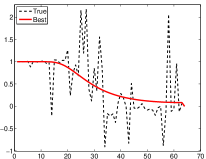
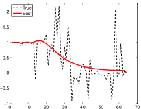
SD	CGLS
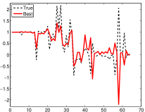
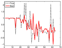
ISRA	HMZ

Figure 2: Comparison of the $\boldsymbol{x}_{\text{true}}$ filter factors (black dashed) for the heat test problem with the ones generated by gradient methods with different scaling matrices at the iteration corresponding to the minimum error (red solid). The nonscaled filters are also reported (SD).

From the reconstruction errors and the filter factors we can make the following remarks:

• as expected, the presence of a scaling matrix provides an acceleration of the algorithms, resulting in a general lower number of iterations required to achieve the best reconstruction. In particular, the well-known fast convergence of the CGLS method is attested by the very few iterations needed;

• the slower convergence seems to help the diagonal scalings ISRA and HMZ in providing better regularized solutions. The improvements in the performances are clearly visible also in the plots of the filter factors. The CGLS filters $\phi_{i}^{k+1}$ ($i=1,\ldots,n$) at each iteration preserve the “regularity” with respect to the index $i$ already observed in Figure 1 for the nonscaled methods. On the contrary, the ISRA and HMZ scalings succeed in reconstructing more faithfully the irregular filters profile of the true solution;

• the effect of the scaling matrix, however, seems to provide some general improvements in the reconstruction errors also for the CGLS matrix, even if the differences with the nonscaled case are minimal. From the plots shown in Figure 2, we can observe that these improvements are due to the slightly better reconstructions of the very first filters, corresponding to the higher singular values.

The same test problem has been used for the analysis of the projected algorithms, since its solution is a non-negative vector. In this case, we considered only the nonscaled method and the diagonal scaling matrices ISRA and HMZ, for which the projection is trivial (see Section 3.3). Moreover, we did not find any difference between the projection schemes (16) and (17), therefore we will present only the results obtained in the latter case. The best reconstruction errors and the corresponding numbers of iterations required by the different algorithms are reported again in Table 2, while the filter factors are plotted in Figure 3. In all cases, the presence of the constraint on the unknown produces a positive effect on the solution, attested by the reported lower reconstruction error. In particular, in the nonscaled case we can observe the irregular filter profile already remarked for the scaled methods, in agreement with the fact that also the presence of a matrix $\boldsymbol{D}_{k}$ makes any filter factor related to all the singular values and singular vectors of the matrix $\boldsymbol{A}$.

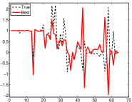
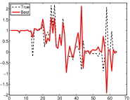
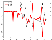
SD_P	ISRA_P	HMZ_P

Figure 3: Comparison of the $\boldsymbol{x}_{\text{true}}$ filter factors (black dashed) for the heat test problem with the ones generated by projected gradient methods with the ISRA and HMZ scaling matrices at the iteration corresponding to the minimum error (red solid). The nonscaled filters are also reported (SD_P).

Very similar considerations hold true also in the second test we carried out and concerning a 2-dimensional dataset. In particular, we used the blur test problem, taken again from Hansen’s Regularization Tools and simulating the degrading effect on a real image due to the action of a general acquisition system (see Figure 4). Here we set $n=256$, thus obtaining the true and measured images of $16\times 16$ pixels. Moreover, we assumed the same parameters for the noise that we chose in the heat case.
A clear figure with the plots of the filter factors for all the considered gradient methods is hard to be produced, due to the irregularity of the filter profiles and the higher number of filters themselves with respect to the 1-dimensional test. However, we noticed again the regular behaviour in the unconstrained problem of the nondiagonal scalings, while the filter factors provided by ISRA and HMZ reproduced more precisely the ones computed with the true image. With the addition of the projection on the non-negative orthant, the reconstruction errors of both the nonscaled and the diagonally scaled algorithms decrease, reflecting the fact that a more faithful representation of the filters leads to a better reconstruction of the true image. In order to appreciate the positive effects on the regularized solutions, for this 2-dimensional case we reported in Figure 4 the restored images by the different algorithms. In particular, we can see that the gradient method with the ISRA scaling is able to remove most artifacts also in the unconstrained case. When the projected algorithms are used, instead, the presence of a scaling matrix seems to provide some benefits only in the reduced number of iterations required, since the best reconstruction error is already achievable with the nonscaled method.

Table 3: Optimal numbers of iterations required by gradient methods with SD steplength and different scaling matrices for solving blur, with the corresponding minimum error. The suffix ‘_P’ denotes the projected algorithms.

Method	Iter	Min err
SD	1199	0.256
CGLS	28	0.223
ISRA	847	0.111
HMZ	1352	0.165
SD_P	1870	0.089
ISRA_P	1590	0.094
HMZ_P	707	0.089

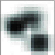
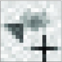
True image	Measured image	SD
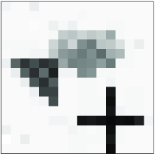
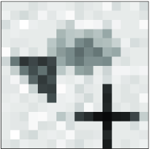
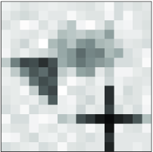
ISRA	HMZ	CGLS
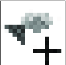
SD_P	ISRA_P	HMZ_P

Figure 4: Comparison of the best reconstructed images for the blur test problem generated by gradient methods with different scaling matrices. The reconstruction with a nonscaled method is also reported (SD). The suffix ‘_P’ denotes the projected algorithms. True object and corresponding blurred noisy image are also showed.

5 Conclusions

In this paper we analyzed the regularizing effect of several gradient methods for the solution of the linear least-squares problem, i.e., the ability of the scheme to produce a sequence of vectors that, at a certain iteration, approximates as close as possible the true solution. The analysis we carried out has been made in terms of the ability of a given method to reproduce correctly the filter factors of the solution, accounting for the way in which the resulting sequence opposes the amplification effect of the noise on the data due to the presence of small singular values. The starting point of our work has been a paper of Nagy & Palmer, in which the filter factors for nonscaled gradient methods have been formally calculated and numerically analyzed. In our paper we extended this analysis to the presence of scaling matrices in defining the descent direction, showing the analytical form of the corresponding filter factors and the advantages that can be obtained not only in terms of efficiency in decreasing the least-squares functional, but also in providing a better approximations of the unknown solution (as remarked e.g. in [8]). Moreover, we also considered the case of non-negative constraints, and we generalized the expression of the filter factors to the projected gradient methods whose projection can be performed by means of the multiplication with a suitable diagonal matrix. We showed on some numerical examples the positive effect of the projection in reconstructing the irregular filter profiles of the true solution, in both scaled and nonscaled cases.

References

- [1] Barzilai, J., Borwein, J.M.: Two point step size gradient methods. IMA J. Numer. Anal. 8(1), 141–148 (1988)
- [2] Bardsley, J., Nagy, J.: Covariance-preconditioned iterative methods for nonnegatively constrained astronomical imaging. SIAM J. Matrix Anal. A. 27(4), 1184–1198 (2006)
- [3] Benvenuto, F., Zanella, R., Zanni, L., Bertero, M.: Nonnegative least-squares image deblurring: improved gradient projection approaches. Inverse Probl. 26(2), 025004 (2010)
- [4] Bertero, M., Boccacci, P.: Introduction to inverse problems in imaging. Institute of Physics, Bristol (1998)
- [5] Bertero, M., Lanteri, H., Zanni, L.: Iterative image reconstruction: a point of view, in Mathematical Methods in Biomedical Imaging and Intensity-Modulated Radiation Therapy (IMRT). (Y. Censor, M. Jiang, and A. K. Louis eds.), Edizioni della Normale, Pisa, Italy, Birkhauser-Verlag, 37–63 (2008)
- [6] Bertsekas, D.P.: Nonlinear Programming. Athena Scientific, Belmont (1999)
- [7] Bonettini, S., Zanella, R., Zanni, L.: A scaled gradient projection method for constrained image deblurring. Inverse Probl. 25(1), 015002 (2009)
- [8] Bonettini, S., Landi, G., Loli Piccolomini, E., Zanni, L.: Scaling techniques for gradient projection-type methods in astronomical image deblurring. Int. J. Comput. Math. 90(1), 9–29 (2013)
- [9] Cauchy, A.: Méthode générale pour la résolution des systèmes d’equations simultanées. C. R. Acad. Sci. Paris 25, 536–538 (1847)
- [10] Dai, Y.H., Yuan, Y.X.: Alternate minimization gradient method. IMA J. Numer. Anal. 23(3), 377–393 (2003)
- [11] Dai, Y.H., Hager, W.W., Schittkowski, K., Zhang, H.: The cyclic Barzilai-Borwein method for unconstrained optimization. IMA J. Numer. Anal. 26(3), 604–627 (2006)
- [12] Daube-Witherspoon, M.E., Muehllener, G.: An iterative image space reconstruction algorithm suitable for volume ECT. IEEE T. Med. Imaging 5(2), 61–66 (1986)
- [13] Donatelli, M., Serra Capizzano, S.: Filter factor analysis of an iterative multilevel regularizing method. Electron. T. Numer. Ana. 29, 163–177 (2008)
- [14] Engl, H.W., Hanke, M., Neubauer, A.: Regularization of inverse problems. Kluwer Academic Publisher, Dordrecht (2000)
- [15] Frassoldati, G., Zanni, L., Zanghirati, G.: New adaptive stepsize selections in gradient methods. J. Indust. Manag. Optim. 4(2), 299–312 (2008)
- [16] Hager, W.W., Bernard, A.M., Zhang, H.: An affine-scaling interior-point CBB method for box-constrained optimization. Math. Program. 119(1), 1–32 (2009)
- [17] Hansen, P.C.: Regularization tools: A Matlab package for the analysis and solution of discrete ill-posed problems. Numer. Algorithms 6(1), 1–35 (1994)
- [18] Hansen, P.C.: Rank-deficient and discrete ill-posed problems. SIAM, Philadelphia (1997)
- [19] Hansen, P.C., Nagy, J.G., O’Leary, D.P.: Deblurring Images: Matrices, Spectra and Filtering. SIAM, Philadelphia (2006)
- [20] Lantéri, H., Roche, M., Cuevas, O., Aime, C.: A general method to devise maximum likelihood signal restoration multiplicative algorithms with non-negativity constraints. Signal Process. 81(5), 945–974 (2001)
- [21] Lantéri, H., Roche, M., Aime, C.: Penalized maximum likelihood image restoration with positivity constraints: multiplicative algorithms. Inverse Probl. 18(5), 1397–1419 (2002)
- [22] Nagy, J., Palmer, K.: Steepest descent, CG and iterative regularization of ill-posed problems. BIT 43(5), 1003–1017 (2003)
- [23] Nocedal, J., Wright, S.J.: Numerical optimization (2nd edition). Springer, New York (2006)
- [24] Prato M., Cavicchioli R., Zanni L., Boccacci P., Bertero M. 2012: Efficient deconvolution methods for astronomical imaging: algorithms and IDL-GPU codes. Astronomy & Astrophysics 539, A133
- [25] Shepp, L.A., Vardi, Y.: Maximum likelihood reconstruction for emission tomography. IEEE T. Med. Imaging 1(2), 113–122 (1982)
- [26] Vogel, C.R.: Computational methods for inverse problems. SIAM, Philadelphia (2002)
- [27] Zhou, B., Gao, L., Dai, Y.H.: Gradient methods with adaptive step-sizes. Comput. Optim. Appl. 35(1), 69–86 (2006)