General theory of feedback control of a nuclear spin ensemble in quantum dots

Abstract

We present a microscopic theory of the nonequilibrium nuclear spin dynamics driven by the electron and/or hole under continuous wave pumping in a quantum dot. We show the correlated dynamics of the nuclear spin ensemble and the electron and/or hole under optical excitation as a quantum feedback loop and investigate the dynamics of the many nuclear spins as a nonlinear collective motion. This gives rise to three observable effects: (i) hysteresis, (ii) locking (avoidance) of the pump absorption strength to (from) the natural resonance, and (iii) suppression (amplification) of the fluctuation of weakly polarized nuclear spins, leading to prolonged (shortened) electron spin coherence time. A single nonlinear feedback function as a “measurement” of the nuclear field operator in the quantum feedback loop is constructed which determines the different outcomes of the three effects listed above depending on the feedback being negative or positive. The general theory also helps to put in perspective the wide range of existing theories on the problem of a single electron spin in a nuclear spin bath.

I Introduction

The nonequilibrium dynamics of the nuclear spins has a long history in spin resonance spectroscopy.Abragam (1961) The recently revived interest in this topic is mostly due to the decoherence issue of the electron spin qubit in semiconductor quantum dots (QDs) for quantum computation.Hanson et al. (2007); Ladd et al. (2010a); Liu et al. (2010) The nuclear spins, abundant in popular III-V semiconductor QDs, produce a randomly fluctuating nuclear field [straight arrow in Fig. 1(a)] that rapidly deprives the electron spin of its phase coherence,Khaetskii et al. (2002); Merkulov et al. (2002); Semenov and Kim (2003); Witzel et al. (2005); Witzel and Das Sarma (2006); Deng and Hu (2006); Yao et al. (2006, 2007); Liu et al. (2007); Yang and Liu (2008a, b, 2009); Cywiński et al. (2009) the wellspring of various advantages of quantum computation over its classical counterpart. Suitable control of the nuclear spin dynamics can suppress the fluctuation of the nuclear field (and hence mitigate the detrimental effect of the electron spin decoherence) and even turn the nuclear spins into a resource to store long-lived quantum information.Kane (1998); Taylor et al. (2003a, b); Witzel and Das Sarma (2007)

In this introduction, we introduce the most widely explored control of the nuclear spin dynamics: dynamic nuclear polarization and more generally, the flip of the nuclear spins by the electron and/or the hole (the removal of an electron from the fully occupied valence band of a semiconductor). This process, followed by the back action of the nuclear spins on the electron and/or hole, forms different feedback loops responsible for a variety of experimental observations, especially the suppression of the nuclear spin fluctuation. First, in Sec. I.1, we introduce dynamic nuclear polarization, the feedback loops, and relevant experimental observations. Then, in Sec. I.2, we briefly survey the electron-nuclear and hole-nuclear interactions and the most general feedback loop constructed from these interactions. Next, in Sec. I.3, we summarize the exitsting theoretical treatments of different feedback loops (especially the back action part). Finally, in Sec. I.4, we introduce our systematic, microscopic theory of the most general feedback loop and summarize the main results.

I.1 Dynamic nuclear polarization and feedback

The simplest control of the nuclear spins is dynamic nuclear polarization, by which a nonequilibrium steady-state nuclear spin polarization $s$ is induced. Then the nuclear field acting on the electron spin [straight arrow in Fig. 1(a)] acquires a nonzero average and its fluctuation is expectedCoish and Loss (2004) to be suppressed to $(1-s^{2})^{1/2}$ of its thermal equilibrium fluctuation, e.g., a $\sim 99\%$ nuclear spin polarization can suppress the nuclear field fluctuation by an order of magnitude and hence prolong the coherence time of the electron spin in the QD by the same factor. This prospect has stimulated intensive interest in dynamic nuclear polarization in the QD. The most widely explored scenario is to transfer the spin angular momenta from the conduction band electron to the nuclear spins [wavy arrow in Fig. 1(a)]Overhauser (1953); Lampel (1968); Paget et al. (1977); Imamoglu et al. (2003); Rudner and Levitov (2007a); Christ et al. (2007); Danon and Nazarov (2008) through the isotropic electron-nuclear contact hyperfine interaction $\propto\mathbf{\hat{S}}_{e}\cdot\mathbf{\hat{I}}$. This scenario has been demonstrated via different processes in various experimental setups, including the two-electron singlet-triplet transition in transport experiments in lateral and vertical double QDs,Ono and Tarucha (2004); Koppens et al. (2005); Deng and Hu (2005); Koppens et al. (2006); Jouravlev and Nazarov (2006); Baugh et al. (2007); Rudner and Levitov (2007b); Petta et al. (2008); Reilly et al. (2008a); Foletti et al. (2009); Gullans et al. (2010); Reilly et al. (2010); Rudner et al. (2010) electron spin resonance in lateral double QDs,Laird et al. (2007); Nowack et al. (2007); Danon et al. (2009) and in particular, interband optical pumping in fluctuation QDs and self-assembled QDs,Brown et al. (1996); Gammon et al. (1997, 2001); Bracker et al. (2005); Yokoi et al. (2005); Lai et al. (2006); Akimov et al. (2006); Eble et al. (2006); Braun et al. (2006); Mikkelsen et al. (2007); Dzhioev and Korenev (2007); Maletinsky et al. (2007a); Tartakovskii et al. (2007); Oulton et al. (2007); Maletinsky et al. (2007b); Kaji et al. (2007, 2008); Belhadj et al. (2009); Ladd et al. (2010b); Krebs et al. (2010); Fallahi et al. (2010); Chekhovich et al. (2010, 2011) where the highest degree of steady-state nuclear spin polarization (up to $\sim 65\%$) has been achieved.Gammon et al. (2001); Bracker et al. (2005); Chekhovich et al. (2010) The nonzero average nuclear field produced by the polarized nuclear spins is then detected as an average energy shift of the electron [straight arrow in Fig. 1(a)]. In many experiments, the average energy shift exhibits hysteretic behaviors, indicating the bistability or multistability of the average nuclear field due to the nonlinear feedback loop [Fig. 1(a)] between the electron and the nuclear spins. Note that, as a convention, the “nuclear spin flip” [e.g., denoted by the wavy arrow in Fig. 1(a)] may or may not have a preferential direction and therefore is more general than dynamic nuclear polarization, which involves nuclear spin flip with a preferential direction.

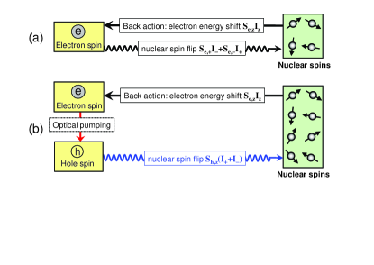
Figure 1: (a) Feedback loop between the electron spin $\mathbf{\hat{S}}_{e}$ and the nuclear spins $\{\mathbf{\hat{I}}_{j}\}$ through the contact hyperfine interaction $\propto\mathbf{\hat{S}}_{e}\cdot\mathbf{\hat{I}}=(\hat{S}_{e,+}\hat{I}_{-}+\hat{S}_{e,-}\hat{I}_{+})/2+\hat{S}_{e,z}\hat{I}_{z}$: the electron flips the nuclear spins (with or without a preferential direction) through $\hat{S}_{e,+}\hat{I}_{-}+\hat{S}_{e,-}\hat{I}_{+}$ (wavy arrow) and changes the nuclear field, which in turn acts back on the electron through $\hat{S}_{e,z}\hat{I}_{z}$ (straight arrow). (b) A specific feedback loop between the electron spin $\mathbf{\hat{S}}_{e}$, the hole spin $\mathbf{\hat{S}}_{h}$, and the nuclear spins $\{\mathbf{\hat{I}}_{j}\}$. First, the hole flips the nuclear spins through the non-collinear dipolar hyperfine interaction $\propto\hat{S}_{h,z}(\hat{I}_{+}+\hat{I}_{-})$ (wavy arrow) and changes the nuclear field. Second, the nuclear field acts on the electron through the diagonal part $\hat{S}_{e,z}\hat{I}_{z}$ of the contact hyperfine interaction (straight arrow). Third, the electron is coupled to the hole through interband optical pumping.

Recently, several experimental groups reported significant suppression of the nuclear field fluctuation for weakly or moderately polarized nuclear spins in QD ensembles,Greilich et al. (2007); Carter et al. (2009) two coupled quantum dots,Reilly et al. (2008b); Bluhm et al. (2010); Barthel et al. (2012); Yao and Luo (2010) and in particular, single quantum dots,Xu et al. (2009); Latta et al. (2009); Vink et al. (2009) an important configuration for quantum computation. In single quantum dots,Xu et al. (2009); Latta et al. (2009); Vink et al. (2009); Sun et al. (2012) the key experimental observation is the maintenance (i.e., locking) of resonant absorption over a range of pump frequency around the natural resonance. This locking behavior arises from the shift of the electron energy level from off-resonance to resonance by the average nuclear field. A striking observation by both Xu et al.Xu et al. (2009) and Latta et al.Latta et al. (2009) is that the locking occurs nearly symmetrically on both sides of the resonance. This symmetric locking reveals that the steady-state nuclear field is antisymmetric across the resonance, a prominent feature beyond the framework of the electron-nuclear contact hyperfine interaction [Fig. 1(a)]. In order to explain this feature, Xu et al.Xu et al. (2009) (followed by Ladd et al.Ladd et al. (2010b, 2011) in a different context) introduced a new feedback loop [Fig. 1(b)] consisting of the nuclear spin flip (with no preferential direction) induced by a valence band hole inside a trion (which consists of two inert conduction band electrons in the spin singlet state and an unpaired valence band hole) and the back action of the nuclear field on the conduction band electron, which is then coupled to the hole by interband optical pumping. Very recently, the mechanism for the hole-driven nuclear spin flip with a preferential direction (i.e., hole-driven dynamic nuclear polarization) through the non-collinear dipolar hyperfine interaction was also establishedYang and Sham (2012) and generalizedHögele et al. (2012); Urbaszek et al. (2013) to the non-collinear electron-nuclear hyperfine interaction to explain the experimentally observed locking and avoidance of the pump absorption strength from resonance.

Figure 2: (a) Feedback processes between the electron spin $\mathbf{\hat{S}}_{e}$, the hole spin $\mathbf{\hat{S}}_{h}$, and the nuclear spins $\{\mathbf{\hat{I}}_{j}\}$. The electron flips the nuclear spins through the off-diagonal contact hyperfine interaction $\propto\hat{S}_{e,+}\hat{I}_{-}+\hat{S}_{e,-}\hat{I}_{+}$ and the non-collinear interaction $\propto\hat{S}_{e,z}(\hat{I}_{+}+\hat{I}_{-})$. The hole flips the nuclear spins through the off-diagonal dipolar hyperfine interaction $\propto\hat{S}_{h,+}\hat{I}_{-}+\hat{S}_{h,-}\hat{I}_{+}$ and the non-collinear dipolar hyperfine interaction $\propto\hat{S}_{h,z}(\hat{I}_{+}+\hat{I}_{-})$. The nuclear spins act back on the electron through the diaognal contact hyperfine interaction $\propto\hat{S}_{e,z}\hat{I}_{z}$, and on the hole through the diagonal dipolar hyperfine interaction $\propto\hat{S}_{h,z}\hat{I}_{z}$. (b) A general feedback loop between the nuclear spins and externally controlled electron and/or hole (hereafter referred to as e-h system for brevity). For the sake of generality, $\hat{F}_{z}$ and $\hat{F}_{+}$ ($=\hat{F}_{-}^{\dagger}$) refer to arbitrary electron or hole operators (not necessarily spin operators). In particular, $\hat{F}_{z}$ does not necessarily refer to $\hat{S}_{e,z}$ or $\hat{S}_{h,z}$ and $\hat{F}_{+}$ does not necessarily refer to $\hat{S}_{e,+}$ or $\hat{S}_{h,+}$.

I.2 General feedback processes between electron, hole, and nuclear spins

To date, the following interactions between the electron, the hole, and the nuclear spins have been considered:

• The isotropic electron-nuclear contact hyperfine interaction $\propto\mathbf{\hat{S}}_{e}\cdot\mathbf{\hat{I}}$, which consists of the diagonal part $\propto\hat{S}_{e,z}\hat{I}_{z}$ and the off-diagonal part $\propto\hat{S}_{e,+}\hat{I}_{-}+\hat{S}_{e,-}\hat{I}_{+}$.

• The anisotropic hole-nuclear dipolar hyperfine interaction,Fischer et al. (2008); Xu et al. (2009); Eble et al. (2009); Testelin et al. (2009); Fallahi et al. (2010); Chekhovich et al. (2011); Yang and Sham (2012) whose dominant part is diagonal $\propto\hat{S}_{h,z}\hat{I}_{z}$. Heavy-light hole mixingBester et al. (2003); Koudinov et al. (2004); Krizhanovskii et al. (2005) introduces a smaller off-diagonal part $\propto\hat{S}_{h,+}\hat{I}_{-}+\hat{S}_{h,-}\hat{I}_{+}$ and an even smaller non-collinear part $\propto\hat{S}_{h,z}(\hat{I}_{+}+\hat{I}_{-})$. This interaction becomes relevant when the valence band hole is excited by interband optical pumping.

• The non-collinear electron-nuclear hyperfine interaction $\propto\hat{S}_{e,z}(\hat{I}_{+}+\hat{I}_{-})$, which exists between the electron of the phosphorus donor in silicon and the ²⁹Si isotope nuclear spins.Saikin and Fedichkin (2003); Witzel et al. (2007) It may also arise in optically excited III-V QDs when the quadrupolar axes of the nuclear spins are not parallel to the external field.Latta et al. (2011)

These interactions enable a variety of feedback processes between the electron, the hole, and the nuclear spins [Fig. 2(a)]. In the general scenario, the nuclear spins can be flipped by both the electron and the hole, through both the pair-wise flip-flop ($\hat{S}_{e,+}\hat{I}_{-}+\hat{S}_{e,-}\hat{I}_{+}$ or $\hat{S}_{h,+}\hat{I}_{-}+\hat{S}_{h,-}\hat{I}_{+}$) and the non-collinear interaction [$\hat{S}_{e,z}(\hat{I}_{+}+\hat{I}_{-})$ or $\hat{S}_{h,z}(\hat{I}_{+}+\hat{I}_{-})$]. The nuclear spins act back on both the electron and the hole through the diagonal interaction ($\hat{S}_{e,z}\hat{I}_{z}$ or $\hat{S}_{h,z}\hat{I}_{z}$). Such feedback processes correlate the dynamics of different nuclear spins and play a critical role in suppressing the nuclear field fluctuation and hence prolonging the electron spin coherence time. In particular, all experimentally reported Greilich et al. (2007); Carter et al. (2009); Reilly et al. (2008b); Bluhm et al. (2010); Barthel et al. (2012); Xu et al. (2009); Latta et al. (2009); Vink et al. (2009) suppressions of the nuclear field fluctuation occur in weakly or moderately polarized systems and are attributed to feedback processes [Fig. 2(a)] instead of a strong nuclear spin polarization. They demonstrate that to suppress the nuclear field fluctuation significantly, constructing a proper feedback loop is more feasible than achieving a strong nuclear spin polarization $s\sim 99\%$, which remains an experimentally demanding goal.

A general feedback loop [Fig. 2(b)] between the electron and the hole (hereafter referred to as e-h system for brevity) and the nuclear spins consists of two steps. First, the e-h system flips the nuclear spins [wavy arrow in Fig. 2(b)] and hence changes the nuclear field. Second, the nuclear field acts back on the e-h system [straight arrow in Fig. 2(b)]. For the first step, perturbation theory is usually sufficient since the hyperfine interaction between the e-h system and the nuclear spins is weak. For the second step, however, the nuclear field acting back on the e-h system must be treated non-perturbatively since it may be comparable with the characteristic energy scale of the electron or hole spin.

I.3 Theoretical treatment of nuclear field back action

In treating the nuclear field back action, many existing theories take into account the average nuclear field but neglect its fluctuation. This approach is capable of reproducing the average nuclear field responsible for the experimentally observed hysteretic or locking behaviors, but provides no information about the nuclear field fluctuation. In addition to numerical simulation,Latta et al. (2009); Issler et al. (2010) different approaches have been utilized to incorporate the nuclear field fluctuation:

• For the electron-nuclei feedback loop [Fig. 1(a)], Rudner and LevitovRudner and Levitov (2007b, 2010) and subsequently Danon and NazarovDanon and Nazarov (2008); Danon et al. (2009); Vink et al. (2009) introduced the stochastic approach for nuclear spin-1/2’s by assuming that the nuclear field experiences a random walk described by a single-variable Fokker-Planck equation. The analytical solution of the Fokker-Planck equation quantifies the nuclear field fluctuation and shows that the competition between dynamic nuclear polarization and nuclear spin depolarization gives rise to a restoring force that can suppress the nuclear field fluctuation well below the thermal equilibrium value.

• For the electron-nuclei feedback loop [Fig. 1(a)] involving nuclear spin flip with no preferential direction, Greilich et al.Greilich et al. (2007) derived a slightly different Fokker-Planck equation by assuming a semi-classical rate equation for the nuclear field distribution for nuclear spin-1/2’s.Barnes and Economou (2011) The solution shows that even if the nuclear spin flip has no preferential direction, a strong feedback suppressing the nuclear field fluctuation can still exist in steady state, in contrast to the stochastic approach, which gives a vanishing feedback in this case.

• For the electron-hole-nuclei feedback loop [Fig. 1(b)], Xu et al. Xu et al. (2009) argued that the dependence of the average nuclear field on the optical detuning (which in turn depends on the fluctuating nuclear field) provides a feedback channel that can significantly suppress the nuclear field fluctuation. This provide an intuitive, qualitative picture for suppressing the nuclear field fluctuation by the feedback loop.

• For the electron-hole-nuclei feedback loop [Fig. 1(b)], our previous studyYang and Sham (2012) established the mechanism of hole-driven dynamic nuclear polarization through the non-collinear dipolar hyperfine interaction [wavy arrow in Fig. 1(b)]. There, motivated by the stochasticRudner and Levitov (2007b, 2010); Danon and Nazarov (2008); Danon et al. (2009); Vink et al. (2009) and rate equationGreilich et al. (2007) approaches, we outlined a microscopic derivation of the Fokker-Planck equation for this specific mechanism without any stochastic or semi-classical assumptions. The analytical solution quantifies the intuitive picture by Xu et al. Xu et al. (2009) and establishes a connection to different approaches.Coish and Loss (2004); Rudner and Levitov (2007b, 2010); Danon and Nazarov (2008); Danon et al. (2009); Vink et al. (2009); Greilich et al. (2007)

The above approaches provide an excellent understanding for certain feedback processes, but still have the drawback that they are constructed for nuclear spin-1/2’s (while the widely explored GaAs and InAs quantum dots all contain nuclei with spins higher than 1/2) or for specific feedback loops [Figs. 1(a) and 1(b)] with specific nuclear spin-flip mechanism (while the identified electron-nuclear and hole-nuclear interactions enable more general feedback processes) and/or they involve certain (stochastic or semi-classical) assumptions. To maximize the control over the nuclear field and its fluctuation by flexible construction of the feedback loop, it is desirable to develop a comprehensive understanding for a general feedback loop and nuclear spin-flip mechanism, such as that shown in Fig. 2(b).

I.4 A systematic, microscopic theory for a general feedback loop

In this paper, we present a systematic, microscopic theory for such a feedback loop [Fig. 2(b)], with the e-h system subjected to continuous wave pumping, an important experimental situation. In particular, we study how this feedback loop controls both the average nuclear field and its fluctuation. This is achieved by decoupling the slow nuclear field dynamics from the fast motion of other dynamical variables (e.g., the off-diagonal nuclear spin coherences and the e-h variables) through the adiabatic approximation, which enables us to incorporate non-perturbatively the back action from the fluctuating nuclear field [straight arrow in Fig. 2(b)]. Our microscopic theory justifies and unifies the stochastic approachRudner and Levitov (2007b, 2010); Danon and Nazarov (2008); Danon et al. (2009); Vink et al. (2009) and the rate equation approachGreilich et al. (2007) and generalizes them to include nuclei with spins higher than 1/2. It identifies two different kinds of steady-state feedback. The “drift” feedback (as considered by the stochastic approachRudner and Levitov (2007b, 2010); Danon and Nazarov (2008); Danon et al. (2009); Vink et al. (2009) and Xu et al.Xu et al. (2009)) originates from the nonlinear drift of the nuclear field, thus its existence requires nuclear spin flip with a preferential direction. By contrast, the “diffusion” feedback (as considered by Greilich et al.Greilich et al. (2007) and Barnes and EconomouBarnes and Economou (2011) in the rate equation approach and Issler et al.Latta et al. (2009); Issler et al. (2010) by numerical simulation) originates from the nonlinear diffusion of the nuclear field, so it remains efficient even when the nuclear spin flip has no preferential direction.

In this paper we focus on the more popular “drift” feedback followed by a brief discussion about the “diffusion” feedback. The control of the “drift” feedback over the nuclear field can be understood from three successive steps. (i) When the feedback loop is broken by neglecting the back action, each nuclear spin is driven by the e-h system independently. (ii) When the feedback loop is closed by taking into account the back action from the average nuclear field, the average nuclear field becomes coupled to the dynamics of different nuclear spins and its motion becomes nonlinear or even multistable. This is responsible for the experimentally observed hysteresis and absorption strength locking or avoidance.Xu et al. (2009); Latta et al. (2009); Vink et al. (2009); Högele et al. (2012) (iii) When the back action from the fluctuating nuclear field is fully taken into account, the fluctuating nuclear field becomes coupled to the dynamics of different nuclear spins, which enables the feedback loop to further control (e.g., suppress or amplify) the nuclear field fluctuation. This is responsible for the experimentally observed suppression of the nuclear field fluctuation and hence prolonged electron spin coherence time.Greilich et al. (2007); Carter et al. (2009); Reilly et al. (2008b); Bluhm et al. (2010); Barthel et al. (2012); Xu et al. (2009); Latta et al. (2009); Vink et al. (2009)

Our key finding is that all the above controls can be quantified concisely by a single nonlinear nuclear field feedback function $\mathbb{H}(h)$. In the feedback loop, an “input” magnetic field $h$ from the nuclear spins [straight arrow in Fig. 2(b)] influences the e-h system, which in turn drives the nuclear spins [wavy arrow in Fig. 2(b)] to a collective mixed state, producing an “output” nuclear field $\mathbb{H}$. Physically, this nonlinear feedback function encapsulates the mutual response between the nuclear field and the e-h system. It provides a unified, quantitative description to three observable effects in the steady state:

1. Hysteresis, which originates from multiple stable average nuclear fields. The average nuclear field $h^{(\mathrm{ss})}$ is determined by the self-consistent equation $h=\mathbb{H}(h)$, which, due to the strong nonlinearity of $\mathbb{H}(h)$, may have multiple solutions $\{h_{\alpha}^{(\mathrm{ss})}\}$ ($\alpha=1,2,\cdots$). Each solution $h_{\alpha}^{(\mathrm{ss})}$ is associated with a nuclear field feedback strength

   $$\mathbb{H}^{\prime}(h_{\alpha}^{(\mathrm{ss})})\equiv\left(\frac{d\mathbb{H}(h)}{dh}\right)_{h=h_{\alpha}^{(\mathrm{ss})}},$$ (1)

   which quantifies the sensitivity of the average “output” nuclear field to the “input” nuclear field. If $\mathbb{H}^{\prime}(h_{\alpha}^{(\mathrm{ss})})<1$, then $h_{\alpha}^{(\mathrm{ss})}$ is a stable average nuclear field associated with a stable feedback and a macroscopic nuclear spin state.

2. Locking (Avoidance) of the pump absorption strength to (from) a certain value.Xu et al. (2009); Latta et al. (2009); Vink et al. (2009) Suppose that the nuclear spins are in a macroscopic state $h_{\alpha}^{(\mathrm{ss})}$ with a feedback strength $\mathbb{H}^{\prime}(h_{\alpha}^{(\mathrm{ss})})$. When the pump frequency $\omega$ changes by $\delta\omega$, the nuclear field will shift the electron or hole excitation energy $\omega_{eh}$ by $\delta\omega_{eh}$, in such a way that the detuning $\Delta\equiv\omega_{eh}-\omega$ (which determines the pump absorption strength) changes by

   $$\delta\Delta=\delta\omega_{eh}-\delta\omega=\frac{-\delta\omega}{1-\mathbb{H}^{\prime}(h_{\alpha}^{(\mathrm{ss})})}.$$

   1. For a strong negative feedback $\mathbb{H}^{\prime}(h_{\alpha}^{(\mathrm{ss})})\ll-1$, we have $\left|\delta\Delta\right|\ll\left|\delta\omega\right|$, i.e., the detuning and hence the pump absorption strength remains nearly constant over a wide range of the pump frequency, corresponding to the locking of the pump absorption strength to a plateau value.

   2. For a strong positive feedback $\mathbb{H}^{\prime}(h_{\alpha}^{(\mathrm{ss})})>1$, the value $h_{\alpha}^{(\mathrm{ss})}$ becomes unstable, leading to the avoidance of the corresponding absorption strength.

   3. For a weak positive feedback $\mathbb{H}^{\prime}(h_{\alpha}^{(\mathrm{ss})})\lesssim 1$, we have $|\delta\Delta|\gg|\delta\omega|$, i.e., the detuning and hence the pump absorption strength changes drastically upon a slight change of the pump frequency, corresponding to the avoidance of the pump absorption strength from a certain value.

3. The suppression or amplification of the nuclear field fluctuation of weakly polarized nuclear spins. In a weakly polarized macroscopic nuclear spin state $h_{\alpha}^{(\mathrm{ss})}$ with a feedback strength $\mathbb{H}^{\prime}(h_{\alpha}^{(\mathrm{ss})})$, the feedback loop changes the nuclear field fluctuation from the thermal equilibrium value $\sigma_{\mathrm{eq}}$ to $\sigma_{\mathrm{eq}}[1-\mathbb{H}^{\prime}(h_{\alpha}^{(\mathrm{ss})})]^{-1/2}$. Thus negative (positive) feedback suppresses (amplifies) the nuclear field fluctuation. Combination of  (ii) and (iii) gives a positive correlation between the absorption strength locking (avoidance) and the suppression (amplification) of the nuclear field fluctuation: the stronger the locking (avoidance), the stronger the suppression (amplification).

By estimating the efficiency of the “drift” feedback and the “diffusion” feedback, we conclude that the feedback approach is capable of suppressing the nuclear field fluctuation to recover the intrinsic electron spin coherence time.

To exemplify our general theory, especially the quantification of the “drift” feedback by the nonlinear feedback function, we consider the feedback loop in Fig. 2(b), initially proposed by Xu et al.Xu et al. (2009) and subsequently explored by our previous studyYang and Sham (2012) that established the mechanism of hole-driven dynamic nuclear polarization through the non-collinear dipolar hyperfine interaction. This feedback loop serves as an excellent example for our general theory because it can realize all the interesting regimes discussed above. In particular, we find a highly nonlinear feedback function that gives rise to bistable macroscopic nuclear spin states. For negative nuclear Zeeman frequency, one state has a strong negative feedback $\mathbb{H}^{\prime}(h_{\alpha}^{(\mathrm{ss})})\ll-1$, leading to strong locking of the pump absorption strength to the resonance and significantly suppressed nuclear field fluctuation. When the nuclear Zeeman frequency is reversed, one state has a positive feedback, leading to strong avoidance of the pump absorption strength from resonance and enhanced nuclear field fluctuation.

II Theory

We consider many nuclear spins coupled to a generic e-h system under continuous wave pumping in a single QD subjected to an external magnetic field $B$ along the $z$ growth axis. The total Hamiltonian is

$$\hat{H}(t)=\hat{H}_{N}+\hat{H}_{eh}(t)+\hat{V}(t).$$ (2)

The nuclear spin Hamiltonian is

$$\hat{H}_{N}\equiv\sum_{j}\omega_{j,N}\hat{I}_{j}^{z},$$ (3)

where $\omega_{j,N}\equiv-\gamma_{j,N}B$ is the nuclear Zeeman frequency and the summation $\sum_{j}$ runs over all nuclear spins in the QD. The e-h Hamiltonian $\hat{H}_{eh}(t)$ includes the continuous pumping and the coupling of the e-h system to the environment (e.g., vacuum electromagnetic fluctuationScully and Zubairy (2002) or neighboring electron/hole reservoirsDreiser et al. (2008)), which introduces damping into the e-h system. The general coupling between the e-h system and the nuclear spins can be written as

$$\hat{V}(t)\equiv\hat{F}_{z}(t)\hat{h}_{z}+\hat{F}_{+}(t)\hat{h}_{-}+\hat{F}_{-}(t)\hat{h}_{+},$$ (4)

where $\hat{F}_{z}(t)=\hat{F}_{z}^{\dagger}(t)$ and $\hat{F}_{-}(t)=\hat{F}_{+}^{\dagger}(t)$ are arbitrary dimensionless operators (not necessarily spin operators) for the electron or the hole. In particular, $\hat{F}_{z}$ does not necessarily refers to $\hat{S}_{e,z}$ or $\hat{S}_{h,z}$ and $\hat{F}_{+}$ does not necessarily refer to $\hat{S}_{e,+}$ or $\hat{S}_{h,+}$. These operators are coupled to different components

$$\hat{h}_{z} \equiv\sum_{j}a_{j,z}\hat{I}_{j,z},$$

$$\hat{h}_{+} \equiv\sum_{j}a_{j,+}\hat{I}_{j,+},$$

and $\hat{h}_{-}=\hat{h}_{+}^{\dagger}$ of the nuclear field, where $\hat{I}_{j,\pm}\equiv\hat{I}_{j,x}\pm i\hat{I}_{j,y}$. The feedback loop in this model corresponds to Fig. 2(b) with $\hat{I}_{\alpha}$ replaced by $\hat{h}_{\alpha}$. Through the off-diagonal coupling

$$\hat{V}_{\mathrm{nd}}(t)\equiv\hat{F}_{+}(t)\hat{h}_{-}+\hat{F}_{-}(t)\hat{h}_{+},$$ (5)

the e-h system flips the nuclear spins [wave arrow in Fig. 2(b)] and changes the nuclear field, which in turn acts back on the e-h system through the diagonal coupling $\hat{F}_{z}(t)\hat{h}_{z}$ [straight arrow in Fig. 2(b)]. To incorporate non-perturbatively the back action by the diagonal coupling, we divide the total Hamiltonian $\hat{H}(t)$ into the diagonal, unperturbed part

$$\hat{H}_{0}(t)\equiv\hat{H}_{N}+\hat{H}_{eh}(t)+\hat{F}_{z}(t)\hat{h}_{z},$$ (6)

to be treated non-perturbatively, and the off-diagonal part $\hat{V}_{\mathrm{nd}}(t)$, to be treated perturbatively.

We are interested in the control of the feedback loop over the nuclear field dynamics, which is associated with the diagonal part $\hat{P}(t)$ of the nuclear spin density matrix. Therefore, we need to single out the motion of $\hat{P}(t)$ from the exact equation of motion

$$\frac{d}{dt}\hat{\rho}(t)=-i[\hat{H}_{0}(t)+\hat{V}_{\mathrm{nd}}(t),\hat{\rho}(t)]$$

for the density matrix $\hat{\rho}(t)$ of the coupled system. This can be achieved by the following time-scale analysis for three essential processes, two being driven by the unperturbed Hamiltonian $\hat{H}_{0}(t)$ and one being driven by the perturbation $\hat{V}_{\mathrm{nd}}(t)$:

1. Dissipative dynamics of the e-h system driven by $\hat{H}_{0}(t)$. Here $\hat{h}_{z}$ may be regarded as a classical parameter since it commutes with every term in $\hat{H}_{0}(t)$. Through the diagonal coupling $\hat{F}_{z}(t)\hat{h}_{z}$ in $\hat{H}_{0}(t)$, the back action of the nuclear field $\hat{h}_{z}$ on the e-h system [straight arrow in Fig. 2(b)] changes the free e-h evolution

   $$\hat{U}_{eh}(t)=\mathcal{T}e^{-i\int_{0}^{t}\hat{H}_{eh}(t^{\prime})dt^{\prime}}$$ (7)

   to a $\hat{h}_{z}$-dependent evolution

   $$\hat{U}_{eh}(\hat{h}_{z},t)=\mathcal{T}e^{-i\int_{0}^{t}[\hat{H}_{eh}(t^{\prime})+\hat{F}_{z}(t^{\prime})\hat{h}_{z}]dt^{\prime}}$$ (8)

   ($\mathcal{T}$ is the time-ordering operator) that establishes a $\hat{h}_{z}$-dependent steady e-h state $\hat{\rho}_{eh}^{(\mathrm{ss})}(\hat{h}_{z},t)=\hat{U}_{eh}(\hat{h}_{z},t)\hat{\rho}_{eh}(0)\hat{U}_{eh}^{\dagger}(\hat{h}_{z},t)$ within the e-h relaxation time $T_{eh}\sim 1\ \mathrm{ns}$Xu et al. (2009) [recall that $\hat{H}_{eh}(t)$ includes the e-h relaxation].

2. Nuclear spin dephasing driven by $\hat{H}_{0}(t)$. Through the diagonal coupling in $\hat{H}_{0}(t)$, the e-h fluctuation eliminates the off-diagonal nuclear spin coherences (see Appendix A for details) within the nuclear spin dephasing time $T_{2,N}\sim 0.01-1\ \mathrm{ms}$. Additional nuclear spin dephasing on the time scale $\sim 0.1\ \mathrm{ms}$ comes from the nuclear-nuclear dipolar interaction.Abragam (1961); Witzel and Das Sarma (2007) This process transforms an arbitrary nuclear spin density matrix $\hat{\rho}_{N}(t)$ to a diagonal one $\hat{P}(t)$ with vanishing nuclear spin coherences.

3. Nuclear spin relaxation driven by $\hat{V}_{\mathrm{nd}}(t)$. Through the off-diagonal coupling, the e-h fluctuation flips the nuclear spins [wavy arrow in Fig. 2(b)] and changes the nuclear field within the nuclear spin relaxation time $T_{1,N}\sim 1-100$ $\mathrm{s}$.Ono and Tarucha (2004); Lai et al. (2006); Laird et al. (2007); Mikkelsen et al. (2007); Greilich et al. (2007); Chekhovich et al. (2010) The decay of the nuclear field due to, e.g., the non-secular part of the nuclear-nuclear dipolar interaction, occurs on the same time scale.Maletinsky et al. (2007a); Baugh et al. (2007); Greilich et al. (2007); Reilly et al. (2008b)

To summarize, the unperturbed evolution driven by $\hat{H}_{0}(t)$ rapidly establish a classically correlated state $\hat{\rho}_{eh}^{(\mathrm{ss})}(\hat{h}_{z},t)\hat{P}(t)$ on a short time scale $\sim T_{eh},T_{2,N}$, while the off-diagonal coupling $\hat{V}_{\mathrm{nd}}(t)$ slowly flips the nuclear spins and changes the nuclear field $\hat{h}_{z}$ on a much longer time scale $\sim T_{1,N}\gg T_{eh},T_{2,N}$. This fact enables us to use the adiabatic approximation to separate the unperturbed evolution from the nuclear spin flip by assuming that the classically correlated state is instantaneously established after each nuclear spin flip. In this case, on the time scale of $T_{1,N}$, we can use the classically correlated state $\hat{\rho}_{eh}^{(\mathrm{ss})}(\hat{h}_{z},t)\hat{P}(t)$ as the zeroth-order approximation to the state of the whole system and incorporate the off-diagonal coupling [wavy arrow in Fig. 2(b)] through the second-order perturbation theory in the density matrix formalism. Through straightforward algebra (see Appendix B for details), we arrive at the following rate equation for $\hat{P}(t)$ up to second order of $\hat{V}_{\mathrm{nd}}$ on the time scale of $T_{1,N}$ under the condition that the e-h fluctuation is invariant under temporal translation:

$$\frac{d}{dt}\hat{P}(t)=-\sum_{j}[\hat{I}_{j,-},\hat{I}_{j,+}W_{j,+}(\hat{h}_{z})\hat{P}(t)]-\sum_{j}[\hat{I}_{j,+},\hat{I}_{j,-}W_{j,-}(\hat{h}_{z})\hat{P}(t)],$$ (9)

where

$$W_{j,\pm}(\hat{h}_{z})=\left|a_{j,+}\right|^{2}\int_{-\infty}^{\infty}e^{\mp i\omega_{j,N}t}dt\ \operatorname*{Tr}\nolimits_{eh}\hat{F}_{\pm}^{\mathrm{I}}(\hat{h}_{z},t)\hat{F}_{\mp}^{\mathrm{I}}(\hat{h}_{z},0)\hat{\rho}_{eh}^{(\mathrm{ss})}(\hat{h}_{z},0)$$ (10)

is the rate of the transition of the $j$th nuclear spin that increases [for $W_{j,+}(\hat{h}_{z})$] or decreases [for $W_{j,-}(\hat{h}_{z})$] the quantum number of $\hat{I}_{j,z}$ by one [Fig. 3(b)] and

$$\hat{O}^{\mathrm{I}}(\hat{h}_{z},t)\equiv\hat{U}_{eh}(\hat{h}_{z},t)\hat{O}(t)\hat{U}_{eh}^{\dagger}(\hat{h}_{z},t)$$ (11)

for an arbitrary e-h operator $\hat{O}(t)$. The e-h fluctuation $\operatorname*{Tr}\nolimits_{eh}\hat{F}_{\pm}^{\mathrm{I}}(\hat{h}_{z},t)\hat{F}_{\mp}^{\mathrm{I}}(\hat{h}_{z},0)\hat{\rho}_{eh}^{(\mathrm{ss})}(\hat{h}_{z},0)$ and hence the transition rates $W_{j,\pm}(\hat{h}_{z})$ can be evaluated through the quantum regression theorem.Scully and Zubairy (2002)

Figure 3: (a) The back action of the nuclear field $\hat{h}_{z}$ (straight arrow) instantaneously establish a $\hat{h}_{z}$-dependent e-h steady state $\hat{\rho}_{eh}^{(\mathrm{ss})}(\hat{h}_{z},t)$, whose fluctuation in turn flips the nuclear spin (wavy arrow) and changes the nuclear field. (b) The spin-flip transition rates $W_{j,\pm}(\hat{h}_{z})$ of the $j$th nuclear spin between adjacent eigenstates $\{\left|m\right\rangle_{j}\}$ of $\hat{I}_{j}^{z}$ are dependent on the nuclear field $\hat{h}_{z}$.

Equation (9) describes the dynamics of the diagonal part of the nuclear spin density matrix (i.e., the population flow of the nuclear spins) driven by the feedback loop. Equation (10) is the non-equilibrium versionDanon and Nazarov (2011) of the fluctuation-dissipation theorem:Gardiner and Zoller (2004) the fluctuation of the non-equilibrium e-h system [driven by the $\hat{h}_{z}$-dependent evolution $\hat{U}_{eh}(\hat{h}_{z},t)$] induces irreversible population flow of the nuclear spins towards a non-equilibrium steady state. Now the entire feedback loop reduces from Fig. 2(b) to Fig. 3(a). First, the “input” nuclear field $\hat{h}_{z}$ acting on the e-h system [straight arrow in Fig. 3(a)] changes the free e-h evolution $\hat{U}_{eh}(t)$ [Eq. (7)] to a $\hat{h}_{z}$-dependent evolution $\hat{U}_{eh}(\hat{h}_{z},t)$ [Eq. (8)] that instantaneously establishes the $\hat{h}_{z}$-dependent e-h steady state $\hat{\rho}_{eh}^{(\mathrm{ss})}(\hat{h}_{z},t)$ and hence e-h fluctuation $\operatorname*{Tr}\nolimits_{eh}\hat{F}_{\pm}^{\mathrm{I}}(\hat{h}_{z},t)\hat{F}_{\mp}^{\mathrm{I}}(\hat{h}_{z},0)\hat{\rho}_{eh}^{(\mathrm{ss})}(\hat{h}_{z},0)$. Second, through the off-diagonal coupling [wavy arrow in Fig. 3(a)], the $\hat{h}_{z}$-dependent e-h fluctuation induces an $\hat{h}_{z}$-dependent irreversible population flow of the nuclear spins [Fig. 3(b)]. Then the “output” nuclear field generated by this population flow depends on the “input” nuclear field $\hat{h}_{z}$. Finally, the back action of this “output” nuclear field on the e-h system [straight arrow in Fig. 3(a)] closes the feedback loop.

Up to now we have neglected the nuclear spin depolarization, e.g., by the nuclear-nuclear dipolar interactions. If these processes do not interfere with the e-h mechanism considered here, then they can be characterized by phenomenological decay rates $\{\Gamma_{j,1}\}$ and incorporated into Eq. (9) by replacing the transition rates $W_{j,\pm}(\hat{h}_{z})$ by $W_{j,\pm}(\hat{h}_{z})+\Gamma_{j,1}/2$. Hereafter it is understood that $W_{j,\pm}(\hat{h}_{z})$ already includes the nuclear spin depolarization.

Our solution of Eq. (9) consists in the control of the average nuclear field and the nuclear field fluctuation by the feedback loop. For simplicity we consider uniform couplings $a_{j,+}=a_{+},a_{j,z}=a_{z}$ (generalization to non-uniform couplings can be achieved by coarse grainingPetrov et al. (2009)) of the e-h system to identical nuclear spin-$I$’s with $\omega_{j,N}=\omega_{N}$ in the QD, so that $W_{j,\pm}(\hat{h}_{z})=W_{\pm}(\hat{h}_{z})$ is independent of $j$. The nuclear field

$$\hat{h}_{z}=\left(NIa_{z}\right)\times\left(\frac{1}{NI}\sum_{j=1}^{N}\hat{I}_{j}^{z}\right)\equiv h_{\max}\hat{s},$$

where $N$ is the total number of nuclear spins in the QD, $h_{\max}\equiv NIa_{z}$ is the nuclear field from fully polarized nuclear spins, and $\hat{s}\equiv\hat{h}_{z}/h_{\max}$ is the polarization per unit nuclear spin or the normalized nuclear field. Hereafter, we will refer to $\hat{s}$ as the nuclear field in cases of no confusion.

The explanation of the feedback control is organized as follows. (A) We start with a nuclear field operator $\hat{h}_{z}$ acting back on the e-h system [straight arrow in Fig. 3(a)] taking a constant value $h$ (as if it were measured) and introduce the notion of a nuclear field feedback function $\mathbb{H}(h)$. (B) We take into account the back action of the average nuclear field, discuss the multistability of the nuclear field, and use the nuclear field feedback strength $\mathbb{H}^{\prime}(h)\equiv d\mathbb{H}(h)/dh$ to quantify the locking (or avoidance) of the pump absorption strength to (or from) a certain value. (C) We close the feedback loop by fully taking into account the back action from the fluctuating nuclear field $\hat{h}_{z}$. In this case, we identify two different kinds of steady-state feedback: the “drift” feedback originating from the nonlinear drift of the nuclear field and the “diffusion” feedback originating from the nonlinear diffusion of the nuclear field. We show that the nuclear field fluctuation controlled by the “drift” feedback is quantified by the nuclear spin polarizationCoish and Loss (2004) (negligible for weakly polarized system) and the feedback strength $\mathbb{H}^{\prime}(h)$. By estimating the efficiency of the “drift” feedback and “diffusion” feedback, we conclude that the feedback approach is capable of suppressing the nuclear field fluctuation to recover the intrinsic electron spin coherence time.

II.1 Back action from constant nuclear field: nuclear field feedback function

Here we assume that the nuclear field $\hat{h}_{z}$ acting on the e-h system takes a constant value $h$, then the e-h induced nuclear spin-flip rate $W_{\pm}(\hat{h}_{z})\rightarrow W_{\pm}(h)$ becomes $c$-numbers as the feedback loop is “measured”. In this case, the dynamics of different nuclear spins are decoupled and the density matrix for all the nuclear spins is the product of the density matrices of individual nuclear spins. The average polarization $\langle\hat{I}_{j}^{z}\rangle/I$ of each nuclear spin is equal to $s(t)\equiv\operatorname*{Tr}\hat{s}\hat{P}(t)$. Therefore, as long as $s(t)$ is concerned, we need only consider one nuclear spin in this case.

For nuclear spin-1/2’s, Eq. (9) gives

$$\frac{d}{dt}s=-\Gamma_{\mathrm{tot}}(h)[s-s_{0}^{(1/2)}(h)],$$ (12)

where

$$s_{0}^{(1/2)}(h)=\frac{W_{+}(h)-W_{-}(h)}{W_{+}(h)+W_{-}(h)}$$ (13)

is the steady-state nuclear spin polarization, established within the nuclear spin relaxation time $T_{1,N}(h)=1/\Gamma_{\mathrm{tot}}(h)$, where $\Gamma_{\mathrm{tot}}(h)\equiv W_{+}(h)+W_{-}(h)$.

For nuclei with a general spin $I$, the steady-state nuclear spin polarization becomes

$$s_{0}(h)\equiv B_{I}\left(I\ln\frac{1+s_{0}^{(1/2)}(h)}{1-s_{0}^{(1/2)}(h)}\right)\approx\frac{2(I+1)}{3}s_{0}^{(1/2)}(h),$$ (14)

where $B_{I}(x)\equiv(2I+1)/(2I)\coth[(2I+1)x/(2I)]-1/(2I)\coth[x/(2I)]$ is the Brillouin function. The real-time motion of $s(t)$ is given by

$$\frac{d}{dt}s =-\Gamma_{\mathrm{tot}}(h)\left(s-\frac{\langle\hat{I}_{j,x}^{2}\rangle+\langle\hat{I}_{j,y}^{2}\rangle}{I}s_{0}^{(1/2)}(h)\right)$$

$$\approx-\Gamma_{\mathrm{tot}}(h)[s-s_{0}(h)].$$ (15)

The last step of Eqs. (14) and (15) is valid if $I=1/2$ or $|s_{0}(h)|\ll 1$. Below, unless explicitly stated, we always consider this situation. Equation (14) shows that for weak polarization $|s_{0}(h)|\ll 1$, the polarization of nuclear spin-$I$’s is enhanced by a factor $\sim 2(I+1)/3$ compared with that of nuclear spin-1/2’s.

The steady state value of the average nuclear field $\operatorname*{Tr}\hat{h}_{z}\hat{P}(t)$ as a function of $h$ is given by a nonlinear function

$$\mathbb{H}(h)\equiv h_{\max}s_{0}(h).$$ (16)

Since the function $\mathbb{H}(h)$ connects the “input” nuclear field $h$ acting on the e-h system [straight arrow in Fig. 3(a)] and the average “output” nuclear field produced by the nuclear spins driven by the e-h fluctuation [wavy arrow in Fig. 3(a)], we call $\mathbb{H}(x)$ the nuclear field feedback function. It encapsulates (i) the nonlinear response of the e-h fluctuation to the nuclear field acting on the e-h system [straight arrow in Fig. 3(a)] and (ii) the response of the nuclear field to the e-h fluctuation [wavy arrow in Fig. 3(b)]. Equation (16) also shows that $s_{0}(h)=\mathbb{H}(h)/h_{\max}$ is just the normalized nuclear field feedback function.

II.2 Back action from average nuclear field: absorption strength locking or avoidance

Here we take into account the average nuclear field $h(t)\equiv\operatorname*{Tr}\hat{P}(t)\hat{h}_{z}$ acting on the e-h system, i.e., $W_{\pm}(\hat{h}_{z})\rightarrow W_{\pm}(h(t))$. In this case, the dynamics of different nuclear spins are coupled to the average nuclear field $h(t)$. This enables the feedback loop to control the average nuclear field. As a result, the motion of $h(t)=h_{\max}s(t)$, as obtained from Eq. (15) by replacing $h$ with $h(t)$, becomes nonlinear:

$$\frac{d}{dt}h(t)\approx-\Gamma_{\mathrm{tot}}(h(t))[h(t)-\mathbb{H}(h(t))].$$ (17)

The average nuclear field $h^{(\mathrm{ss})}$ in the steady state is determined by the self-consistent equation $h=\mathbb{H}(h)$, which, due to the nonlinearity of $\mathbb{H}(h)$, may have multiple solutions $\{h_{\alpha}^{(\mathrm{ss})}\}$ (distinguished by the subscript $\alpha=1,2,\cdots$). Each solution $h_{\alpha}^{(\mathrm{ss})}$ is associated with a nuclear field feedback strength $\mathbb{H}^{\prime}(h_{\alpha}^{(\mathrm{ss})})$, as defined in Eq. (1). A positive (negative) feedback corresponds to $\mathbb{H}^{\prime}(h_{\alpha}^{(\mathrm{ss})})>0$ [$\mathbb{H}^{\prime}(h_{\alpha}^{(\mathrm{ss})})<0$]. The equation of motion for the deviation $\delta h_{\alpha}(t)\equiv h(t)-h_{\alpha}^{(\mathrm{ss})}$ of the average nuclear field $h(t)$ from the $\alpha$-th steady-state value $h_{\alpha}^{(\mathrm{ss})}$ follows from Eq. (17) as

$$\frac{d}{dt}\delta h_{\alpha}\approx-\Gamma_{\mathrm{tot}}(h_{\alpha}^{(\mathrm{ss})})[1-\mathbb{H}^{\prime}(h_{\alpha}^{(\mathrm{ss})})]\delta h_{\alpha}+O[(\delta h_{\alpha})^{2}].$$ (18)

For $h_{\alpha}^{(\mathrm{ss})}$ to be stable, the corresponding feedback strength must satisfy $\mathbb{H}^{\prime}(h_{\alpha}^{(\mathrm{ss})})<1$, so that any deviation of the average nuclear field away from its steady-state value $h_{\alpha}^{(\mathrm{ss})}$ would decay to zero within the nuclear spin relaxation time $T_{1,N}(h_{\alpha}^{(\mathrm{ss})})=1/\Gamma_{\mathrm{tot}}(h_{\alpha}^{(\mathrm{ss})})$. In this case, $h_{\alpha}^{(\mathrm{ss})}$ corresponds to a macroscopic nuclear spin state. For weak nuclear spin polarization, since $s_{0}\approx 2(I+1)s_{0}^{(1/2)}/3$ and $\mathbb{H}=h_{\max}s_{0}=Na_{z}Is_{0}$, we have $\mathbb{H}^{\prime}(h_{\alpha}^{(\mathrm{ss})})\propto I(I+1)$, i.e., nuclei with higher spin have stronger feedback strength.

Recently, under continuous wave pumping, several groupsXu et al. (2009); Latta et al. (2009); Vink et al. (2009) observed the locking of the pump absorption strength to the resonance: when gradually sweeping the pump frequency $\omega$ away from the resonance with the electron or hole excitation, the nuclear field tends to compensate this change and shift the electron or hole excitation energy to restore the resonance. Very recently, the opposite behavior (i.e., pushing the pump absorption strength away from the natural resonance) was predictedYang and Sham (2012) and observed.Högele et al. (2012) These behaviors originate from the feedback of the average nuclear field. Below we use the nuclear field feedback function to quantify these (and more general) behaviors.

In a typical continuous pumping experiment, the back action of an average nuclear field $h$ on the e-h system shifts the electron or hole excitation energy from $\omega_{eh}^{0}$ to $\omega_{eh}\equiv\omega_{eh}^{0}+h$ or $\omega_{eh}\equiv\omega_{eh}^{0}-h$. For specificity we first consider the former case $\omega_{eh}=\omega_{eh}^{0}+h$. The detuning between the electron or hole excitation energy and the pump frequency is $\Delta\equiv\omega_{eh}-\omega=\omega_{eh}^{0}+h-\omega$. Typically the nuclear spin transition rates $W_{\pm}$ (due to e-h fluctuation) are nonlinear functions of $\Delta$ and this is the only source for the dependence of the nuclear field feedback function on $h$. In this case, the feedback function can be written as $\mathbb{H}(h)=\mathcal{H}(\omega_{eh}^{0}+h-\omega)$. Suppose that at an initial pump frequency $\omega$, the nuclear spins are in the $\alpha$-th macroscopic state with an average nuclear field $h_{\alpha}^{(\mathrm{ss})}$ determined by

$$h_{\alpha}^{(\mathrm{ss})}=\mathcal{H}(\omega_{eh}^{0}+h_{\alpha}^{(\mathrm{ss})}-\omega),$$ (19)

the electron or hole excitation energy is $\omega_{eh}=\omega_{eh}^{0}+h_{\alpha}^{(\mathrm{ss})}$, and the detuning is $\Delta=\omega_{eh}^{0}+h_{\alpha}^{(\mathrm{ss})}-\omega$. Now the pump frequency changes by $\delta\omega$ (which is not necessarily small), then the nuclear field changes by $\delta h_{\alpha}^{(\mathrm{ss})}$ determined by

$$h_{\alpha}^{(\mathrm{ss})}+\delta h_{\alpha}^{(\mathrm{ss})}=\mathcal{H}(\omega_{eh}^{0}+h_{\alpha}^{(\mathrm{ss})}+\delta h_{\alpha}^{(\mathrm{ss})}-\omega-\delta\omega),$$ (20)

the electron or hole excitation energy changes by $\delta\omega_{eh}=\delta h_{\alpha}^{(\mathrm{ss})}$, and the detuning changes by $\delta\Delta=\delta\omega_{eh}-\delta\omega$. If the detuning change $\delta\Delta$ is small, then we can make a first-order Taylor expansion to $\mathcal{H}(\omega_{eh}^{0}+h_{\alpha}^{(\mathrm{ss})}+\delta h_{\alpha}^{(\mathrm{ss})}-\omega-\delta\omega)=\mathcal{H}(\omega_{eh}^{0}+h_{\alpha}^{(\mathrm{ss})}-\omega+\delta\Delta)$ and obtain

$$\delta\omega_{eh} =-\frac{\mathbb{H}^{\prime}(h_{\alpha}^{(\mathrm{ss})})}{1-\mathbb{H}^{\prime}(h_{\alpha}^{(\mathrm{ss})})}\delta\omega,$$ (21)

$$\delta\Delta =\frac{-\delta\omega}{1-\mathbb{H}^{\prime}(h_{\alpha}^{(\mathrm{ss})})}.$$ (22)

For the nuclear field shifting the electron or hole excitation energy from $\omega_{eh}^{0}$ to $\omega_{eh}\equiv\omega_{eh}^{0}-h$, Eqs. (21) and (22) still hold.

Equation (22) shows that the feedback loop controls the sensitivity of the pump detuning $\Delta$ [and hence the pump absorption strength $\chi(\Delta)$] to the change of the pump frequency (for clarity we assume that the nuclear field shifts the electron or hole excitation energy from $\omega_{eh}^{0}$ to $\omega_{eh}\equiv\omega_{eh}^{0}+h$ although the same conclusions apply to the opposite case $\omega_{eh}\equiv\omega_{eh}^{0}-h$):

• If $h_{\alpha}^{(\mathrm{ss})}$ is associated with a strong negative feedback $\mathbb{H}^{\prime}(h_{\alpha}^{(\mathrm{ss})})\ll-1$, then the nuclear field induced shift of the electron or hole excitation energy $\delta\omega_{eh}\approx\delta\omega$ [Eq. (21)] largely compensates the change of the pump frequency, so that the change of the detuning $\left|\delta\Delta\right|=\left|\delta\omega_{eh}-\delta\omega\right|\ll\left|\delta\omega\right|$ [Eq. (22)] is very small, which in turn justifies the first-order Taylor expansion to $\mathcal{H}(\omega_{eh}^{0}+h_{\alpha}^{(\mathrm{ss})}-\omega+\delta\Delta)$ [used to derive Eqs. (21) and (22)] even when $\delta\omega$ is not small. As a result, the absorption strength becomes insensitive to the change of the pump frequency. Therefore, the feedback loop with a strong negative feedback serves as a “trap” of the absorption strength: once a strong negative feedback $\mathbb{H}^{\prime}(h_{\alpha}^{(\mathrm{ss})})\ll-1$ is formed at a certain pump frequency $\omega$, further change of the pump frequency over a wide range does not appreciably change the detuning from the value $\omega_{eh}^{0}+h_{\alpha}^{(\mathrm{ss})}-\omega$ and hence does not change the pump absorption strength from the value $\chi(\omega_{eh}^{0}+h_{\alpha}^{(\mathrm{ss})}-\omega)$. The experimentally observedXu et al. (2009); Latta et al. (2009); Vink et al. (2009) locking of the pump absorption strength to the resonance corresponds to the occurance of such a “trap” around the resonance point: $\omega_{eh}^{0}+h_{\alpha}^{(\mathrm{ss})}-\omega=0$ (see Sec. III.2.1 for an example).

• If $h_{\alpha}^{(\mathrm{ss})}$ is associated with a strong positive feedback $\mathbb{H}^{\prime}(h_{\alpha}^{(\mathrm{ss})})>1$, then $h_{\alpha}^{(\mathrm{ss})}$ is unstable, thus the corresponding pump absorption value $\chi(\omega_{eh}^{0}+h_{\alpha}^{(\mathrm{ss})}-\omega)$ will not be observed experimentally in steady state, i.e., the pump absorption value $\chi(\omega_{eh}^{0}+h_{\alpha}^{(\mathrm{ss})}-\omega)$ is avoided. The experimentally observedHögele et al. (2012) avoidance of the pump absorption strength from the resonance corresponds to the occurance of such a unstable feedback on the resonance point: $\omega_{eh}^{0}+h_{\alpha}^{(\mathrm{ss})}-\omega=0$ (see Sec. III.2.2 for an example).

• If $h_{\alpha}^{(\mathrm{ss})}$ is associated with a stable, positive feedback $0<\mathbb{H}^{\prime}(h_{\alpha}^{(\mathrm{ss})})<1$, then the nuclear spin induced shift of the electron or hole excitation energy $\delta\omega_{eh}$ has an opposite sign to the pump frequency change $\delta\omega$, so that $|\delta\Delta|>|\delta\omega|$. Therefore, if a stable, positive feedback $\mathbb{H}^{\prime}(h_{\alpha}^{(\mathrm{ss})})\approx 1$ is formed at a certain pump frequency $\omega$, then even a small change of the pump frequency will lead to drastic change of the nuclear field, which in turn shifts the detuning far away from the expected value $\omega_{eh}^{0}+h_{\alpha}^{(\mathrm{ss})}-\omega$, corresponding to rapid pushing of the pump absorption strength away from the value $\chi(\omega_{eh}^{0}+h_{\alpha}^{(\mathrm{ss})}-\omega)$ (see Sec. III.2.3 for an example).

II.3 Back action from fluctuating nuclear field: suppression or amplification of nuclear field fluctuation

Here we close the feedback loop by fully incorporating the back action of the fluctuating nuclear field $\hat{h}_{z}$. In this case, the dynamics of different nuclear spins are coupled to $\hat{h}_{z}$ through the $\hat{h}_{z}$-dependent transition rates $W_{\pm}(\hat{h}_{z})$. This enables the feedback loop to control the nuclear field, both its average value and its fluctuation. For the paradigmatic central spin model consisting of a confined electron spin coupled to the nuclear spins through the contact hyperfine interaction

$$\hat{V}_{eN}=\sum_{j}a_{j,e}\mathbf{\hat{S}}_{e}\cdot\mathbf{\hat{I}}_{j},$$ (23)

we identify $\hat{F}_{z}\equiv\hat{S}_{e,z}$ and the nuclear field $\hat{h}_{z}\equiv\sum_{j}a_{j,e}\hat{I}_{j,z}$, whose strong fluctuation leads to the detrimental effect of rapid electron spin decoherence.Khaetskii et al. (2002); Merkulov et al. (2002); Semenov and Kim (2003); Witzel et al. (2005); Witzel and Das Sarma (2006); Deng and Hu (2006); Yao et al. (2006, 2007); Liu et al. (2007); Yang and Liu (2008a, b, 2009); Cywiński et al. (2009) Suppressing the nuclear field fluctuation is a major direction of recent research in spin based quantum computation.

The diagonal nuclear spin density matrix $\hat{P}(t)$ contains the information for the population of every nuclear spin, but it is difficult to obtain such microscopic details by solving Eq. (9), even in the steady state, because different nuclear spins are coupled to the fluctuating nuclear field $\hat{h}_{z}$. Fortunately, the quantity of importance is the nuclear field $\hat{h}_{z}=h_{\max}\hat{s}$. Therefore, the key is to single out the dynamics of the nuclear field from Eq. (9), as motivated by the stochasticRudner and Levitov (2007b, 2010); Danon and Nazarov (2008); Danon et al. (2009); Vink et al. (2009) and rate equationGreilich et al. (2007) approaches. For this purpose, we define the probability distribution function $p(s,t)\equiv\operatorname*{Tr}\delta_{\hat{s},s}\hat{P}(t)$ of $\hat{s}$, i.e., the probability for the nuclear field $\hat{s}$ to be equal to $s$ at time $t$. From Eq. (9), we can approximately derive (see Appendix C for details) a closed equation of motion, i.e., the Fokker-Planck equation for $p(s,t)$:

$$\frac{\partial}{\partial t}p(s,t)=\frac{\partial}{\partial s}\left[\frac{\partial}{\partial s}D(s)p(s,t)-v(s)p(s,t)\right],$$ (24)

where

$$D(s)\approx\frac{1}{2NI}\Gamma_{\mathrm{tot}}(h_{\max}s)\left(\frac{2(I+1)}{3}-ss_{0}^{(1/2)}(h_{\max}s)\right)$$ (25)

is the diffusion coefficient and

$$v(s)\approx-\Gamma_{\mathrm{tot}}(h_{\max}s)[s-s_{0}(h_{\max}s)]$$ (26)

is the drift coefficient. The steady-state solution is given by

$$p^{(\mathrm{ss})}(s)=\frac{D(s^{\ast})}{D(s)}p^{(\mathrm{ss})}(s^{\ast})\exp\left(\int_{s^{\ast}}^{s}\frac{v(s^{\prime})}{D(s^{\prime})}ds^{\prime}\right),$$ (27)

where $s^{\ast}$ is an arbitrary constant. The steady-state distribution function $p^{(\mathrm{ss})}(s)$ contains all the information for the nuclear field. Each peak of $p^{(\mathrm{ss})}(s)$ corresponds to a macroscopic nuclear spin state (distinguished by subscript $\alpha$): the position $s_{\alpha}^{(\mathrm{ss})}$ of the $\alpha$-th peak gives the average nuclear field $s_{\alpha}^{(\mathrm{ss})}$, while the width $\sigma_{\alpha}$ of the $\alpha$-th peak quantifies the fluctuation of the nuclear field $\hat{s}$ around its average value $s_{\alpha}^{(\mathrm{ss})}$.

Equations (24)-(27) justify and unify the stochastic approachRudner and Levitov (2007b, 2010); Danon and Nazarov (2008); Danon et al. (2009); Vink et al. (2009) and the rate equation approachGreilich et al. (2007) and generalize them to include nuclei with spins higher than 1/2. For nuclear spin-1/2, the drift coefficient $v(s)$, the diffusion coefficient $D(s)$, and the exponent in Eq. (27) coincide with the stochastic approach,Rudner and Levitov (2007b, 2010); Danon and Nazarov (2008); Danon et al. (2009); Vink et al. (2009) while the factor $D(s^{\ast})/D(s)$ coincides with the rate equation approach.Greilich et al. (2007) The exponent is associated with the nonlinear drift $v(s)$ of the nuclear field, while the factor $D(s^{\ast})/D(s)$ is associated with the nonlinear diffusion $D(s)$ of the nuclear field. They correspond to two distinct feedback processes controlling the nuclear field. As shown below, the feedback originating from the nonlinear drift (hereafter referred to as “drift” feedback) vanishes when the nuclear spin flip has no preferential direction (i.e., $W_{+}=W_{-}$). By contrast, the feedback originating from the nonlinera diffusion (hereafter referred to as “diffusion” feedback) remains efficient even for nuclear spin flip with no preferential direction.

The rest of this subsection is organized as follows. First, we focus on quantifying the “drift” feedback by the nuclear field feedback function. Second, we briefly discuss the “diffusion” feedback. Finally, with the estimate of the efficiency of the “drift” feedback and “diffusion” feedback, we conclude that the feedback is capable of recovering the intrinsic electron spin coherence time.

II.3.1 “Drift” feedback

The “drift” feedback associated with the exponent of $p^{(\mathrm{ss})}(s)$ has been discussed by the stochastic approachRudner and Levitov (2007b, 2010); Danon and Nazarov (2008); Danon et al. (2009); Vink et al. (2009) for nuclear spin-1/2’s. Here we focus on quantifying the control over the nuclear field $\hat{h}_{z}=h_{\max}\hat{s}$ by the “drift” feedback with our nuclear field feedback function for nuclei with a general spin.

Without the factor $D(s^{\ast})/D(s)$, the extremum of $p^{(\mathrm{ss})}(s)$ is determined by $v(s)=0$ as $s=s_{0}(h_{\max}s)$, equivalent to the self-consistent equation $h=h_{\max}s_{0}(h)=\mathbb{H}(h)$ for the average nuclear field since $h=h_{\max}s$. Further, the condition $v^{\prime}(s_{\alpha}^{(\mathrm{ss})})\equiv[dv(s)/ds]_{s=s_{\alpha}^{(\mathrm{ss})}}<0$ for an extremum at $s_{\alpha}^{(\mathrm{ss})}$ to be a peak gives $[ds_{0}(h_{\max}s)/ds]_{s=s_{\alpha}^{(\mathrm{ss})}}<1$, equivalent to the stability condition $\mathbb{H}^{\prime}(h_{\alpha}^{(\mathrm{ss})})<1$ since $h_{\alpha}^{(\mathrm{ss})}=h_{\max}s_{\alpha}^{(\mathrm{ss})}$. Therefore, the conditions determining the average nuclear field and its stability are exactly the same as the mean-field treatment discussed in Sec. II.2, where the nuclear field feedback function provides a complete description. According to the analysis there, $h=\mathbb{H}(h)$ may have multiple stable solutions $\{h_{\alpha}^{(\mathrm{ss})}\}$, corresponding to multiple peaks of $p^{(\mathrm{ss})}(s)$ at $\{s_{\alpha}^{(\mathrm{ss})}\equiv h_{\alpha}^{(\mathrm{ss})}/h_{\max}\}$ and hence multiple macroscopic nuclear spin states.

The key quantity of interest is the fluctuation of the nuclear field $\hat{s}=\hat{h}_{z}/h_{\max}$ in each macroscopic state, as quantified by the width of the probability distribution $p^{(\mathrm{ss})}(s)$ around each peak. For the fluctuation of the nuclear field around its average value $s_{\alpha}^{(\mathrm{ss})}$ in the $\alpha$-th macroscopic state, we follow the stochastic approachRudner and Levitov (2007b, 2010); Danon and Nazarov (2008); Danon et al. (2009); Vink et al. (2009) and expand $v(s)$ around $s_{\alpha}^{(\mathrm{ss})}$ to the first order $v(s)\approx v^{\prime}(s_{\alpha}^{(\mathrm{ss})})(s-s_{\alpha}^{(\mathrm{ss})})$. Then the exponential factor becomes a Gaussian peak $\exp[-(s-s_{\alpha}^{(\mathrm{ss})})^{2}/(2\sigma_{\alpha}^{2})]$ centered at $s_{\alpha}^{(\mathrm{ss})}$. The width of this peak is $\sigma_{\alpha}=[D(s_{\alpha}^{(\mathrm{ss})})/|v^{\prime}(s_{\alpha}^{(\mathrm{ss})})|]^{1/2},$ which, for nuclear spin-1/2’s, coincides with the stochastic approach. By substituting Eqs. (25) and (26) into $\sigma_{\alpha}$, we obtain

$$\sigma_{\alpha}=\sigma_{\mathrm{eq}}\sqrt{\frac{1-[s_{0}^{(1/2)}(h_{\alpha}^{(\mathrm{ss})})]^{2}}{1-\mathbb{H}^{\prime}(h_{\alpha}^{(\mathrm{ss})})}},$$ (28)

where $\sigma_{\mathrm{eq}}\equiv[(I+1)/(3NI)]^{1/2}$ is the thermal equilibrium fluctuation of the nuclear field $\hat{s}$. Note that the normalization $|s_{0}^{(1/2)}|\leq 1$ and the stability condition $\mathbb{H}^{\prime}(h_{\alpha}^{(\mathrm{ss})})<1$ ensures that the quantity inside the square root of Eq. (28) is always finite and non-negative.

Equation (28) shows that in the $\alpha$-th macroscopic nuclear spin state, the nuclear field fluctuation is controlled by the nuclear spin polarization and the feedback:

1. In the absence of the e-h system, we have $s_{0}^{(1/2)}(h)=\mathbb{H}(h)=\mathbb{H}^{\prime}(h)=0$ and hence a unique, vanishing nuclear field $s^{(\mathrm{ss})}=0$ in steady state. The fluctuation of the nuclear field $\hat{s}$ is given by Eq. (28) as $\sigma_{\mathrm{eq}}$, i.e., the thermal equilibrium fluctuation.

2. If we take into account the e-h induced nuclear spin flip [wavy arrow in Fig. 2(b)] but neglect the back action of the nuclear field on the e-h system [straight arrow in Fig. 2(b)], then the dynamics of different nuclear spins is decoupled. In steady state, each individual nuclear spin acquires a finite polarization $s_{0}^{(1/2)}(0)$ that suppresses its own fluctuation by a factor $\sqrt{1-[s_{0}^{(1/2)}(0)]^{2}}$. The fluctuation of the collective nuclear field is suppressed by the same factor.

3. Inclusion of the back action of the average nuclear field (Sec. II.2) leads to multiple stable nuclear fields $\{s_{\alpha}^{(\mathrm{ss})}\}$, so that the suppression of the nuclear field fluctuation around $s_{\alpha}^{(\mathrm{ss})}$ becomes $\sqrt{1-[s_{0}^{(1/2)}(h_{\alpha}^{(\mathrm{ss})})]^{2}}$. Points (2) and (3) describe the suppression of the nuclear field fluctuation by nuclear spin polarization.Coish and Loss (2004)

4. If we fully take into account the back action of the fluctuating nuclear field, then in addition to the factor $\sqrt{1-[s_{0}^{(1/2)}(h_{\alpha}^{(\mathrm{ss})})]^{2}}$ associated with the polarization $s_{0}^{(1/2)}(h_{\alpha}^{(\mathrm{ss})})$ of each individual nuclear spin, the nuclear field fluctuation is further controlled by the feedback, as quantified by the factor $[1-\mathbb{H}^{\prime}(h_{\alpha}^{(\mathrm{ss})})]^{-1/2}$ in Eq. (28). It can either suppress [for negative feedback $\mathbb{H}^{\prime}(h_{\alpha}^{(\mathrm{ss})})<0$] or amplify [for positive feedback $0<\mathbb{H}^{\prime}(h_{\alpha}^{(\mathrm{ss})})<1$] the nuclear field fluctuation without changing the fluctuation of each individual nuclear spin. This quantifies a previous qualitative argumentXu et al. (2009) of feedback induced suppression of the nuclear field fluctuation: when the fluctuation increases (decreases) the nuclear field above (below) its macroscopic value, the negative feedback decreases (increases) the nuclear field and tends to restore its macroscopic value.

II.3.2 “Diffusion” feedback

The “drift” feedback is associated with the peaks $\{s_{\alpha}^{(\mathrm{ss})}\}$ of $p^{(\mathrm{ss})}(s)$ originating from its exponent. One distinguishing feature of the “drift” feedback is that it vanishes when the nuclear spin flip has no preferential direction, i.e., when $W_{+}(h)=W_{-}(h)$. This is because $W_{+}(h)=W_{-}(h)$ leads to vanishing nuclear field feedback function $\mathbb{H}(h)\propto s(h)=0$. Consequently, the self-consistent condition $h=\mathbb{H}(h)$ gives a unique, vanishing steady-state nuclear field and vanishing control over the nuclear field fluctuation, so that $\sigma=\sigma_{\mathrm{eq}}$ [Eq. (28)]. Correspondingly, the exponent reduces to the thermal equilibrium distribution $\exp[-s^{2}/(2\sigma_{\mathrm{eq}}^{2})]$.

By contrast, the “diffusion” feedback is associated with the peaks $\{\bar{s}_{\alpha}^{(\mathrm{ss})}\}$ of $p^{(\mathrm{ss})}(s)$ originating from the sharp dips of $D(s)$. Therefore, it does not vanish even for nuclear spin flip with no preferential direction. Again, the peak of $p^{(\mathrm{ss})}(s)$ at $\bar{s}_{\alpha}^{(\mathrm{ss})}$ corresponds to a macroscopic nuclear spin state with average nuclear field $\bar{s}_{\alpha}^{(\mathrm{ss})}$. The fluctuation $\bar{\sigma}_{\alpha}$ of the nuclear field around the average value $\bar{s}_{\alpha}^{(\mathrm{ss})}$ is determined by the width of the peak. For example, the nuclei induced frequency focusing observed by Greilich et al.Greilich et al. (2007) upon periodic pulsed excitation of the electron spin originates from such “diffusion” feedback. There, $D(s)$ exhibits multiple sharp dips spaced by $2\pi\nu_{\mathrm{rep}}/h_{\max}$ as determined by the pulse repetition rate $\nu_{\mathrm{rep}}$. Recently, based on the electron-induced nuclear spin flip with no preferential direction, Issler et al.Issler et al. (2010) proposed a nuclear spin cooling scheme with nuclear field selective coherent population trapping, where the suppression of the nuclear field fluctuation was analyzed with Monte Carlo simulation. This scheme is an excellent example of the “diffusion” feedback: the coherent dark state dip of the electron population introduces a sharp dip into the electron-induced nuclear spin flip rates $W_{\pm}(h_{\max}s)$ and hence the diffusion coefficient $D(s)$. Consequently, the distribution function $p^{(\mathrm{ss})}(s)$ exhibits a narrow peak, corresponding to a finite nuclear field with suppressed fluctuation.

II.3.3 Recovering intrinsic electron spin coherence time by feedback

First we estimate the efficiency of the “drift” feedback and the “diffusion” feedback. Suppose that the characteristic scale for the nuclear spin transition rates $W_{\pm}(h)$ to change appreciably is $\delta h$. For the “drift” feedback, the maximal feedback strength is roughly estimated as $|\mathbb{H}^{\prime}(h)|\sim h_{\max}/\delta h$, where we have assumed that the maximal achievable nuclear spin polarization $\sim O(1)$. Therefore, according to Eq. (28), the typical fluctuation of the nuclear field $\hat{h}_{z}$ under the “drift” feedback is

$$h_{\max}\sigma\sim\sqrt{a_{z}\delta h}.$$

On the other hand, the typical width $\bar{\sigma}$ of a dip of $D(s)$ is given by the characteristic scale for $D(s)$ to change, i.e., $\bar{\sigma}\sim\delta h/h_{\max}$, thus the typical fluctuation of the nuclear field $\hat{h}_{z}$ under the “diffusion” feedback is

$$h_{\max}\bar{\sigma}\sim\delta h.$$

Note that $h_{\max}\sigma\propto\sqrt{\delta h}$ and $h_{\max}\bar{\sigma}\propto\delta h$ scales differently with $\delta h$.

Second we compare the efficiency of the “drift” feedback with the “diffusion” feedback. If $\delta h\ll a_{z}$, i.e., the nuclear spin flip rates $W_{\pm}(h)$ change drastically upon a slight change of the nuclear field induced by a single nuclear spin flip event, then $h_{\max}\bar{\sigma}\ll h_{\max}\sigma\ll a_{z}$, i.e., the “diffusion” feedback is more efficient. In this case, the rate of the electron spin decoherence due to the nuclear field fluctuation is much smaller than $a_{z}$. In the opposite case $\delta h\gg a_{z}$, we have $h_{\max}\bar{\sigma}\gg h_{\max}\sigma\gg a_{z}$, i.e., the “drift” feedback is more efficient. In this case, the rate of the electron spin decoherence due to nuclear field fluctuation is much larger than $a_{z}$.

Since $W_{\pm}(h)$ are determined by the e-h fluctuation, the typical scale $\delta h$ for $W_{\pm}(h)$ to change appreciably is the relevant e-h relaxation rate $\gamma_{eh}$. Typically the orbital relaxation of the e-h system is much faster than their spin relaxation, thus the smallest $\gamma_{eh}$ corresponds to the “intrinsic” electron or hole spin relaxation rate $1/T_{2,e}$ or $1/T_{2,h}$. Therefore, as long as the limit $\delta h\sim 1/T_{2,e}$ is achieved, the “diffusion” feedback can suppress the nuclear field fluctuation to $h_{\max}\bar{\sigma}\sim 1/T_{2,e}$ and hence recover the intrinsic electron spin coherence time $T_{2,e}$. On the other hand, if $a_{z}\ll 1/T_{2,e}$, then achievement of $\delta h\sim 1/T_{2,e}$ also enables the “drift” feedback to suppress the nuclear field fluctuation to $h_{\max}\sigma\sim\sqrt{a_{z}/T_{2,e}}\ll 1/T_{2,e}$ and hence recover $T_{2,e}$.

III Example: nuclear spin dynamics through non-collinear dipolar hyperfine interaction

To exemplify our general theory, we consider the electron-hole-nuclei feedback loop in Fig. 1(b). It was first proposed by Xu et al.Xu et al. (2009) to explain the experimentally observed symmetric locking of the pump absorption strength and suppressed nuclear field fluctuation, and the key element of this loop, i.e., the mechanism of hole-driven dynamic nuclear polarization, was established recently.Yang and Sham (2012) While Ref. Yang and Sham, 2012 introduced the concept of the feedback loop for this single spin with spin bath problem, the current work differs from it in the perspective of a general theory providing key insight into the important consequences. Here, instead of explicitly classifying the density matrix elements into the “slow” ones and the “fast” ones (which is rather tedious), we directly apply the general result Eq. (10) to the electron-hole-nuclei feedback loop and utilize the quantum regression theorem for a compact derivation. This feedback loop was also utilized by Ladd et al.Ladd et al. (2010b, 2011) to explain the experimentally observed hysteretic sawtooth pattern in the electron spin free induction decay. An advantage of exemplifying our theory with this feedback loop instead of the more intensively investigated electron-nuclei feedback loop [Fig. 1(a)], is that this loop can realize all the interesting regimes discussed in our general theory, i.e., bistability, strong negative feedback, and positive feedback.

The essential difference between the electron-hole-nuclei feedback loop [Fig. 1(b)] and the electron-nuclei feedback loop [Fig. 1(a)] is that in Fig. 1(b), the nuclear spins are flipped by the non-collinear interaction $\propto\hat{S}_{h,z}(\hat{I}_{+}+\hat{I}_{-})$ with the hole, while in Fig. 1(a), the nuclear spins are flipped by the contact hyperfine interaction $\propto\hat{S}_{e,+}\hat{I}_{-}+\hat{S}_{e,-}\hat{I}_{+}$ with the electron. The former process is not accompanied by the hole spin flip, so it involves a very small energy mismatch ($\sim$ nuclear Zeeman splitting) and hence is nearly resonant. By contrast, the latter process is accompanied by the electron spin flip, so it involves a much larger energy mismatch ($\sim$ electron Zeeman splitting) and hence is off-resonant. Consequently, although the hole-nuclear non-collinear interaction is much weaker than the electron-nuclear contact hyperfine interaction, the tremendous resonant enhancement originating from a small energy mismatch could make the strength of the former process comparable with the latter process.Yang and Sham (2012) Recently, this mechanism is generalized to the case of non-collinear electron-nuclear interaction (which arises from nuclear quadrupolar effect Huang and Hu (2010)) to explain the experimentally observed avoidance of resonant absorption Latta et al. (2011). Under optical excitation conditions, both the electron-nuclear and hole-nuclear non-collinear hyperfine interaction may play a role in determining the nuclear polarization. However, the relative contributions from the electron and the hole remains an open issue.Urbaszek et al. (2013)

For the realistic physical system corresponding to the electron-hole-nuclei feedback loop [Fig. 1(b)], we consider a negatively charged QD subjected to an external magnetic field $B$ along the QD growth direction (defined as the $z$ axis). A right circularly polarized continuous wave laser applied in the Faraday configuration couples the spin-up electron level $\left|0\right\rangle$ to the spin-up trion level $\left|1\right\rangle$. The spin-up trion consists of two inert electrons in the spin singlet and one unpaired spin-up hole. Since the hole is the only active member of the trion, hereafter we refer to the trion as hole for brevity. The electron level $\left|0\right\rangle$ and the hole level $\left|1\right\rangle$ form the e-h system illustrated in Fig. 1(b). The optically pumped e-h system is described by the Hamiltonian

$$\hat{H}_{eh}(t)=-\omega_{0}\hat{\sigma}_{00}+\frac{\Omega_{R}}{2}\left(\hat{\sigma}_{10}e^{-i\omega t}+\hat{\sigma}_{01}e^{i\omega t}\right)+\hat{H}_{\mathrm{damp}},$$

where $\omega_{0}$ is the “bare” e-h excitation energy in the absence of the nuclear spins, $\hat{\sigma}_{ji}\equiv\left|j\right\rangle\left\langle i\right|$, $\omega$ is the laser frequency, $\hat{H}_{\mathrm{damp}}$ denotes the coupling to the vacuum electromagnetic fluctuation that leads to spontaneous emission $\left|1\right\rangle\rightarrow\left|0\right\rangle$ with rate $\gamma_{1}$ and hole dephasing with total rate $\gamma_{2}$ in the Lindblad form, and $\Omega_{R}=-e\mathbf{E}_{0}\cdot\left\langle 1\right|\mathbf{r}\left|0\right\rangle$ is the Rabi frequency: the coupling between the electric dipole $-e\left\langle 1\right|\mathbf{r}\left|0\right\rangle$ and the pump electric field $\mathbf{E}(t)=\mathbf{E}_{0}\cos\omega t$. The coupling between the e-h system and the nuclear spins, after being projected into the relevant hilbert space spanned by $\{\left|0\right\rangle$,$\left|1\right\rangle\}$, is

$$\hat{V}=\frac{1}{2}\hat{\sigma}_{00}\sum_{j}a_{j,e}\hat{I}_{j,z}+\hat{\sigma}_{11}\sum_{j}\tilde{a}_{j,h}(\hat{I}_{j,+}+\hat{I}_{j,-}),$$

where the first term is the diagonal part of the electron-nuclear contact hyperfine interaction [leading to the nuclear field back action, as denoted by the straight arrow in Fig. 1(b)] and the second term is the non-collinear part of the hole-nuclear dipolar hyperfine interaction [leading to nuclear spin flip, as denoted by the wavy arrow in Fig. 1(b)]. A brief summary of the nuclear spin dynamics driven by other parts of the electron-nuclear and hole-nuclear interactions could be found elsewhere.Yang and Sham (2012) The total Hamiltonian $\hat{H}(t)=\hat{H}_{N}+\hat{H}_{eh}(t)+\hat{V}$ assumes the same form as our theory [Eq. (2)], where $\hat{H}_{N}$ is the nuclear spin Hamiltonian given in Eq. (3).

To apply our theory to this model, we further put the coupling $\hat{V}$ into the same form as our theory [Eq. (4)] by identifying $\hat{F}_{z}(t)=\hat{\sigma}_{00}$, $\hat{F}_{\pm}(t)=\hat{\sigma}_{11}$, $a_{j,z}=a_{j,e}/2$, and $a_{j,\pm}=\tilde{a}_{j,h}$. Then, according to our theory, after adiabatically eliminating the e-h dynamics, the diagonal part $\hat{P}(t)$ of the nuclear spin density matrix obeys Eq. (9), where the transition rate $W_{j,\pm}(\hat{h}_{z})$ is equal to Eq. (10) plus $\Gamma_{1,j}/2$, which accounts for the nuclear spin depolarization due to other nuclear spin relaxation mechanisms.

As in the general theory, we consider identical nuclear spins ($I_{j}=I$, $\omega_{j,N}=\omega_{N}$, and $\Gamma_{1,j}=\Gamma_{1}$) uniformly coupled to the electron and the hole ($a_{j,e}=a_{e}$, $\tilde{a}_{j,h}=\tilde{a}_{h}$). For a typical self-assembled QD containing $N=10^{4}$ nuclear spins subjected to an external magnetic field $B\sim 1$ T, the order of magnitude of relevant parametersLiu et al. (2007); Xu et al. (2009); Latta et al. (2009); Yang and Sham (2012) is listed in Table 1.

Table 1: Order of magnitude of relevant parameters (unit: $\mathrm{ns}^{-1}$, with the convention $\hbar=1$ understood) for a typical self-ensembled QD containing $N=10^{4}$ nuclear spins under a magnetic field $B\sim$ 1 T.

$\Omega_{R}$	$\gamma_{1}$	$\gamma_{2}$	$\left|\omega_{N}\right|$	$a_{e}$	$\left|\tilde{a}_{h}\right|$	$\Gamma_{1}$
$1$	$1$	$1$	$0.1$	$10^{-2}$	$10^{-5}$	$10^{-10}$

For the present model, the nuclear spin transition rates $W_{\pm}(h)$ and hence the diffusion coefficient $D(s)$ do not exhibit sharp dips, so the “diffusion” feedback is negligible. In the rest, we only consider the “drift” feedback. First we calculate the nuclear field feedback function $\mathbb{H}(h)$. Then we use it to quantify the “drift” feedback (including absorption strength locking or avoidance and the suppression or amplification of the nuclear field fluctuation) for three cases: strong negative feedback, strong positive feedback, and weak positive feedback.

III.1 Nuclear field feedback function

Following the theory in Sec. II.1, to obtain the nuclear field feedback function $\mathbb{H}(h)$, we need the nuclear spin flip rates $W_{\pm}(h)=\tilde{a}_{h}^{2}C(h,\mp\omega_{N})+\Gamma_{1}/2$, where $\hat{h}_{z}$ has been replaced by a constant $h$ and, from Eq. (10),

$$C(h,\nu)\equiv\int_{-\infty}^{\infty}e^{i\nu t}dt\ \operatorname*{Tr}\nolimits_{eh}\hat{\sigma}_{11}^{\mathrm{I}}(h,t)\hat{\sigma}_{11}^{\mathrm{I}}(h,0)\hat{\rho}_{eh}^{(\mathrm{ss})}(h,0).$$

We note that for the present model, the $h$-dependent e-h evolution $\hat{U}_{eh}(h,t)$ [see Eq. (8)] is obtained from the free e-h evolution $\hat{U}_{eh}(t)$ [see Eq. (7)] by replacing the “bare” e-h excitation energy $\omega_{0}$ with the actual e-h excitation energy $\omega_{0}-h$ or equivalently, by replacing the nominal detuning $\Delta_{0}\equiv\omega_{0}-\omega$ with the actual detuning $\Delta\equiv\Delta_{0}-h$. So $C(h,\nu)$ is obtained from $C(h=0,\nu)$ by replacing $\Delta_{0}$ with $\Delta$, i.e., $C(h,\nu)$ is a function of $\Delta$ and $\nu$. Therefore, the $h$-dependence of $C(h,\nu)$ and hence other $h$-dependent quantities such as $s_{0}(h)$ and $\mathbb{H}(h)\equiv h_{\max}s_{0}(h)$ entirely comes from their dependence on $\Delta$. To emphasize this dependence, we use functions of $\Delta$ for functions of $h$, e.g., $C(\Delta,\nu)$ for $C(h,\nu)$, $s_{0}(\Delta)$ for $s_{0}(h)$, and $\mathbb{H}(\Delta)$ for $\mathbb{H}(h)$, etc.

In the absence of the nuclear spin depolarization $(\Gamma_{1}=0$), Eq. (13) gives the steady-state nuclear spin polarization

$$s_{0}^{(1/2\mathrm{)}}(\Delta)=\frac{C(\Delta,-\omega_{N})-C(\Delta,\omega_{N})}{C(\Delta,-\omega_{N})+C(\Delta,\omega_{N})}$$

for nuclear spin-1/2’s. For nuclear spin-$I$’s, the steady-state nuclear spin polarization $s_{0}(\Delta)$ is obtained from Eq. (14) or $s_{0}(\Delta)\approx[2(I+1)/3]s_{0}^{(1/2\mathrm{)}}(\Delta)$ for weak polarization $\left|s_{0}(\Delta)\right|\ll 1$. In the presence of nuclear spin depolarization, $s_{0}^{(1/2\mathrm{)}}(\Delta)$ is reduced by a factor $1+\Gamma_{1}/\Gamma_{p}(\Delta)$ determined by the ratio between the hole-induced nuclear spin flip rate $\Gamma_{p}(\Delta)=\tilde{a}_{h}^{2}[C(\Delta,-\omega_{N})+C(\Delta,\omega_{N})]$ and the nuclear spin depolarization rate $\Gamma_{1}$. For $\Gamma_{1}=0$, by evaluating $C(\Delta,\nu)$ (see Appendix D) through the quantum regression theorem,Scully and Zubairy (2002) we obtain explicit analytical experessions

$$\Gamma_{p}(\Delta) \approx\frac{4\tilde{a}_{h}^{2}\gamma_{1}W(\Delta)}{[\gamma_{1}+2W(\Delta)]^{3}}c_{1}(\Delta),$$ (29)

$$s_{0}^{(1/2)}(\Delta) \approx-\frac{\Delta\omega_{N}}{\Delta^{2}+\gamma_{2}^{2}}\frac{\gamma_{1}}{\gamma_{2}}\frac{c_{0}(\Delta)}{c_{1}(\Delta)},$$ (30)

up to leading order of the small quantity $\varepsilon\equiv\omega_{N}/\gamma_{1,2}$, where $c_{0}(\Delta)=\gamma_{2}/\gamma_{1}+1/2+f(\Delta)+W(\Delta)/\gamma_{1}$ and $c_{1}(\Delta)=1+[\gamma_{1}/(2\gamma_{2})]f(\Delta)+W(\Delta)/\gamma_{1}$ are non-negative constants (because $\gamma_{2}\geq\gamma_{1}/2$) with $f(\Delta)\equiv(\gamma_{2}^{2}-\Delta^{2})/(\gamma_{2}^{2}+\Delta^{2})$ and $W(\Delta)=2\pi(\Omega_{R}/2)^{2}\delta^{(\gamma_{2})}(\Delta)$ is the optical pumping rate from level $\left|0\right\rangle$ to level $\left|1\right\rangle$, with $\delta^{(\gamma_{2})}(\Delta)\equiv$ $(\gamma_{2}/\pi)/(\Delta^{2}+\gamma_{2}^{2})$ the energy-conserving $\delta$-function broadened by hole dephasing. Near resonance $\Delta=0$, we estimate $\Gamma_{p}\sim\tilde{a}_{h}^{2}/\gamma_{1}\sim 0.1$ $\mathrm{s}^{-1}$ to be comparable with the typical nuclear spin depolarization rate $\Gamma_{1}$ (see Table 1).

Figure 4: (color online). $s_{0}(\Delta)$ (solid curves) and $\mathbb{H}^{\prime}(\Delta)/500$ (dotted curves) vs. detuning $\Delta$ for nuclear spin-9/2’s (e.g., InAs QD) for $\Gamma_{1}=0$, (a) $\omega_{N}=-0.1$ $\mathrm{ns}^{-1}$ and (b) $\omega_{N}=0.1$ $\mathrm{ns}^{-1}$. Other parameters are from Table 1. Dark (Black and blue) segments of the curves correspond to stable feedback $\mathbb{H}^{\prime}(\Delta)<1$. Light (Orange) segments correspond to unstable feedback $\mathbb{H}^{\prime}(\Delta)>1$. The straight lines denote $(\Delta_{0}-\Delta)/h_{\max}$, whose intersections with $s_{0}(\Delta)$ give the steady-state nuclear field $\{s_{\alpha}^{(\mathrm{ss})}\},$ including stable (filled circles) and unstable (empty squares) ones.

Equations (29) and (30) are the key results of the recently established mechanism of dynamic nuclear polarization by non-collinear hyperfine interaction.Yang and Sham (2012) In addition to the dependence $s_{0}^{(1/2)}(\Delta),s_{0}(\Delta)\sim\Delta$ responsible for the absorption strength locking or avoidance,Yang and Sham (2012) another distinguishing feature of this mechanism is that in the absence of nuclear spin depolarization $(\Gamma_{1}=0)$, the steady-state nuclear spin polarization $s_{0}(\Delta)$ and hence the nuclear field feedback function $\mathbb{H}(\Delta)=h_{\max}s_{0}(\Delta)$ still strongly depend on the optical detuning $\Delta=\Delta_{0}-h$, so that the “drift” feedback as quantified by the feedback strength $\mathbb{H}^{\prime}(\Delta)=d\mathbb{H}(\Delta)/dh=-d\mathbb{H}(\Delta)/d\Delta=-h_{\max}ds_{0}(\Delta)/d\Delta$ remains efficient, as shown in Fig. 4. By contrast, for other dynamic nuclear polarization mechanisms such as the Overhauser or reverse Overhauser effect,Overhauser (1953); Rudner and Levitov (2007a); Danon and Nazarov (2008); Danon et al. (2009) if $\Gamma_{1}=0$, then $s_{0}(\Delta)$ and hence $\mathbb{H}(\Delta)$ are independent of $\Delta$, so that the “drift” feedback vanishes (as mentioned in the introduction, the stochastic approach constructed for those mechanisms shows that suppression of the nuclear field fluctuation comes entirely from the competition between dynamic nuclear polarization and nuclear spin depolarization). In other words, the “drift” feedback is extrinsic to those mechanisms but intrinsic to the dynamic nuclear polarization induced by non-collinear hyperfine interaction. Below we focus on this intrinsic “drift” feedback by setting $\Gamma_{1}=0$.

In addition to the specific results in Fig. 4, we can also analyze $s_{0}(\Delta)$ and $\mathbb{H}^{\prime}(\Delta)$ more generally. First, $s_{0}^{(1/2)}(\Delta)$, $s_{0}(\Delta)$, and $\mathbb{H}^{\prime}(\Delta)$ are reversed upon reversal of the Zeeman frequency $\omega_{N}$. Second, by dropping the $O(1)$ factors of $(\gamma_{1}/\gamma_{2})c_{0}(\Delta)/c_{1}(\Delta)$ in Eq. (29), we obtain the maximal magnitude of $s_{0}^{(1/2)}(\Delta)$:

$$\left|s_{0}^{(1/2)}\right|_{\max}\sim\frac{\left|\omega_{N}\right|}{\gamma_{2}}.$$

The typical magnitude is $|s_{0}^{(1/2)}|_{\max}\sim 10\%$ (based on Table 1). Third, near the resonance $\left|\Delta\right|\ll\gamma_{2}$, $s_{0}^{(1/2)}(\Delta)\propto\Delta$ is linear in $\Delta$ and the feedback strength is maximal:

$$\mathbb{H}^{\prime}(0)\sim I(I+1)\frac{Na_{e}}{\gamma_{2}}\frac{\omega_{N}}{\gamma_{2}},$$

where we have used $s_{0}(\Delta)\sim(I+1)s_{0}^{(1/2)}(\Delta)$. Based on Table 1, the typical magnitude is $|\mathbb{H}^{\prime}(0)|\sim 10I(I+1)$. Thus the feedback near the resonance is strongly negative (positive) for negative (positive) nuclear Zeeman frequency $\omega_{N}$. These results agree with Fig. 4.

III.2 Back action from nuclear field

We consider three cases: (i) strong negative feedback [$\omega_{N}=-0.1$, Fig. 4(a)], (ii) strong positive feedback [$\omega_{N}=0.1$, Fig. 4(b)], and (iii) weak positive feedback. Case (iii) can be realized by considering nuclear spin-1/2’s (instead of nuclear spin-9/2’s) with a larger hole dephasing rate $\gamma_{2}$. The back action of the nuclear field induces three effects: bistability, absorption strength locking or avoidance, and suppression or amplification of the nuclear field fluctuation. In the following, we illustrate these three effects for each case.

III.2.1 Strong negative feedback

Figure 5: (color online). Steady-state (a) nuclear field $h^{(\mathrm{ss})}$, (b) detuning $\Delta^{(\mathrm{ss})}\equiv\Delta_{0}-h^{(\mathrm{ss})}$, and (c) feedback strength $\mathbb{H}^{\prime}$ vs. nominal detuning $\Delta_{0}$ for $\omega_{N}=-0.1$ $\mathrm{ns}^{-1}$ and $I=9/2$. Other parameters are from Table 1. Dark (Black and blue) segments of the curves correspond to stable feedback $\mathbb{H}^{\prime}<1$. Light (Orange) segments correspond to unstable feedback $\mathbb{H}^{\prime}>1$. (d) Solid curve: steady-state distribution $p^{(\mathrm{ss})}(s)$ of the nuclear field $\hat{s}$ at $\Delta_{0}=10$ $\mathrm{ns}^{-1}$ [marked by dashed straight lines in panels (a)-(c)]. The thermal equilibrium distribution (dotted curve) is also shown for comparison. The unit of the nuclear spin polarization is $\sigma_{\mathrm{eq}}=[(I+1)/(3NI)]^{1/2}$, the thermal equilibrium fluctuation.

Here we consider negative nuclear Zeeman frequency $\omega_{N}=-0.1$ $\mathrm{ns}^{-1}$ [Fig. 4(a)], corresponding to a strong negative feedback near the resonance $\Delta=0$.

For each nominal detuning $\Delta_{0}$, the steady-state nuclear field $h^{(\mathrm{ss})}=h_{\max}s^{(\mathrm{ss})}$ is determined by the nonlinear equation $h=\mathbb{H}(\Delta_{0}-h)$ or equivalently $s=s_{0}(\Delta_{0}-h_{\max}s)$, i.e., $s^{(\mathrm{ss})}$ corresponds to the intersections of $s_{0}(\Delta)$ and $(\Delta_{0}-\Delta)/h_{\max}$ [Fig. 4(a)], where $\Delta\equiv\Delta_{0}-h=\Delta_{0}-h_{\max}s$. For vanishing $h_{\max}$ and hence vanishing feedback strength $\mathbb{H}^{\prime}=0$, we have a unique solution $s^{(\mathrm{ss})}=s_{0}(\Delta_{0})$. For large $h_{\max}$ and hence strong feedback, $(\Delta_{0}-\Delta)/h_{\max}$ becomes less steep and has up to three intersections with $s_{0}(\Delta)$, corresponding to three steady-state nuclear fields. The stability condition $\mathbb{H}^{\prime}<1$ gives $d\mathbb{H}(\Delta)/d\Delta>-1$, i.e., the slope of $s_{0}(\Delta)=\mathbb{H}(\Delta)/h_{\max}$ should be larger than that of $(\Delta_{0}-\Delta)/h_{\max}$. So the three steady-state nuclear fields consist of two stable ones [filled circles in Fig. 4(a)] separated by a unstable one [empty square in Fig. 4(a)].

These steady-state nuclear fields vs. the nominal detuning $\Delta_{0}$ are shown in Fig. 5(a). A striking feature is that in the middle segment (crossed by the dashed line), over a wide range of the nominal detuning $\Delta_{0}\sim[-60$ $\mathrm{ns}^{-1},60$ $\mathrm{ns}^{-1}]$, the stable nuclear field $h^{(\mathrm{ss})}$ follows $\Delta_{0}$ as $h^{(\mathrm{ss})}\approx\Delta_{0}$, so that the steady-state detuning $\Delta^{(\mathrm{ss})}=\Delta_{0}-h^{(\mathrm{ss})}$ is locked to resonance $\Delta^{(\mathrm{ss})}\approx 0$ [Fig. 5(b)]. As discussed in Sec. II.2, this behavior originates from the strong negative feedback $\mathbb{H}^{\prime}(\Delta)\ll-1$ that occurs near $\Delta\approx 0$ [Fig. 4(a)].

The strong locking of $\Delta^{(\mathrm{ss})}$ to resonance $\Delta^{(\mathrm{ss})}\approx 0$ over $\Delta_{0}\sim[-60$ $\mathrm{ns}^{-1},60$ $\mathrm{ns}^{-1}]$ in turn keeps the nuclear field feedback strength $\mathbb{H}^{\prime}(\Delta^{(\mathrm{ss})})\approx\mathbb{H}^{\prime}(0)$ strongly negative over the same range of $\Delta_{0}$ [Fig. 5(c)], although strong negative feedback $\mathbb{H}^{\prime}(\Delta)\ll-1$ only appears over $\Delta\sim[-1$ ns${}^{-1},1$ ns${}^{-1}]$. This strong negative feedback over a wide range of $\Delta_{0}$ in turn strongly suppresses the nuclear field fluctuation over the same range of $\Delta_{0}$ according to Eq. (28). For example, at $\Delta_{0}=10$ $\mathrm{ns}^{-1}$ [marked by the straight dashed line in Figs. 5(a)-5(c)], the detuning is still locked to resonance $\Delta^{(\mathrm{ss})}\approx 0$, so the feedback is still strongly negative. Correspondingly, the width of the peak of $p^{(\mathrm{ss})}(s)$ [solid curve in Fig. 5(d)], which quantifies the nuclear field fluctuation under the feedback control, is much narrower than the width of the thermal distribution [dotted curve in Fig. 5(d)].

III.2.2 Strong positive feedback

Figure 6: (color online). The same as Fig. 5, except that $\omega_{N}=0.1$ $\mathrm{ns}^{-1}$. In panel (d), the two peaks (marked by filled and empty circles) and the dip (marked by empty square) of $p^{(\mathrm{ss})}(s)$ correspond, respectively, to the two stable solutions and the unstable solution in panels (a)-(c) (marked by corresponding symbols).

Here we consider positive nuclear Zeeman frequency $\omega_{N}=0.1$ $\mathrm{ns}^{-1}$ [Fig. 4(b)], corresponding to a strong positive (and hence unstable) feedback near the resonance $\Delta=0$.

In this case, for each nominal detuning $\Delta_{0}$, $(\Delta_{0}-\Delta)/h_{\max}$ could also have up to three intersections with the curve $s_{0}(\Delta)$ [Fig. 4(b)], corresponding to three steady-state nuclear fields $\{h_{\alpha}^{(\mathrm{ss})}\}$, consisting of two stable ones [filled circles in Fig. 4(b)] separated by a unstable one [empty square in Fig. 4(b)].

These steady-state nuclear fields vs. the nominal detuning $\Delta_{0}$ are shown in Fig. 6(a). As a result of the strong positive feedback $\mathbb{H}^{\prime}(\Delta)\gg 1$ near $\Delta\approx 0$ [Fig. 4(b)], although the unstable (and hence not observable) nuclear field (marked by the empty square) follows the nominal detuning $\Delta_{0}$ and locks the detuning $\Delta^{(\mathrm{ss})}=\Delta_{0}-h^{(\mathrm{ss})}$ to resonance, the two stable nuclear fields (marked by empty and filled circles) always push the detuning $\Delta^{(\mathrm{ss})}$ away from resonance, so that resonant absorption is avoided at the natural resonance $\Delta_{0}=0$.

The feedback associated with these two stable solutions are weakly negative and hence, according to Eq. (28), do not appreciably change the nuclear field fluctuation. For example, at $\Delta_{0}=10$ $\mathrm{ns}^{-1}$ [marked by empty and filled circles in Fig. 6(a)-6(c)], the widths of the two peaks of $p^{(\mathrm{ss})}(s)$ [solid curve in 6(d)] are not appreciably changed relative to the peak of the thermal equilibrium distribution [dotted curve in Fig. 6(d)].

III.2.3 Weak positive feedback

Figure 7: (color online). The same as Fig. 6, except that $I=1/2$ and $\gamma_{2}=1.8$ $\mathrm{ns}^{-1}$. In panel (b), the nominal detuning (dotted straight line) is also shown for comparison. In panel (d), the peak of $p^{(\mathrm{ss})}(s)$ correspond to the stable solution at $\Delta_{0}=0$ in panels (a)-(c) (marked by empty circles).

For $\omega_{N}=0.1$ $\mathrm{ns}^{-1}$, to realize weak positive feedback $\mathbb{H}^{\prime}(\Delta)\lesssim 1$ near the resonance $\Delta=0$, we decrease the magnitude of the feedback strength by considering nuclear spin-1/2’s instead of nuclear spin-9/2’s and a larger hole dephasing rate $\gamma_{2}=1.8$ $\mathrm{ns}^{-1}$.

In this case, since the feedback strength is small, the steady-state nuclear field $h^{(\mathrm{ss})}$ [Fig. 7(a)] is unique and does not exhibit bistability. At $\Delta=0$ [marked by the empty circle in Fig. 7(a)-7(c)], the stable steady-state nuclear field $h^{(\mathrm{ss})}$ vanishes, so the resonance condition $\Delta^{(\mathrm{ss})}=\Delta_{0}-h^{(\mathrm{ss})}$ and hence resonant absorption is achieved at natural resonance $\Delta_{0}=0$. However, due to the feedback strength $\mathbb{H}^{\prime}(0)\approx 1$, a slight change of $\Delta_{0}$ (or equivalently the pump frequency) away from zero will drastically change the nuclear field [Fig. 7(a)] and hence the detuning $\Delta^{(\mathrm{ss})}$ [Fig. 7(b)] away from zero, corresponding to large push-away from the natural resonance upon a slight change of the pump frequency (Sec. II.2).

At $\Delta_{0}=0$, the feedback strength $\mathbb{H}^{\prime}(0)\approx 1$ [Fig. 7(c)]. According to Eq. (28), the nuclear field fluctuation is strongly enhanced, as can be seen from the much wider peak of $p^{(\mathrm{ss})}(s)$ [solid curve in Fig. 7(d)] compared with the peak of the thermal equilibrium distribution [dotted curve in Fig. 7(d)].

IV Conclusion

We have developed a microscopic theory for the control of the nuclear field dynamics by a general feedback loop mediated by the electron and/or the hole (referred to as e-h system for brevity) under continuous wave pumping in a quantum dot. This feedback loop consists of two steps. First, the nuclear spins produce a quantum magnetic field $\hat{h}_{z}$ acting on the e-h system [straight arrow in Fig. 3(a)] and establishes a $\hat{h}_{z}$-dependent steady e-h state and hence $\hat{h}_{z}$-dependent e-h fluctuation. Second, through a nonequilibrium fluctuation-dissipation relation, the e-h fluctuation induces an irreversible nuclear spin population flow [wavy arrow in Fig. 3(a)], which in turn changes the nuclear field $\hat{h}_{z}$. By coupling the dynamics of individual nuclear spins to the collective nuclear field $\hat{h}_{z}$, this feedback loop gains control over the average nuclear field and the nuclear field fluctuation. This control leads to three experimentally observed effects: (i) hysteresis in the pump absorption strength; (ii) locking (avoidance) of the pump absorption strength to (from) a certain value; (iii) suppression or amplification of the nuclear field fluctuation, leading to prolonged or shortened electron spin coherence time. By adiabatically eliminating the fast e-h motion in favor of the slow nuclear field dynamics through the adiabatic approximation, we have found that all these three effects can be quantified concisely by a single nonlinear nuclear field feedback function $\mathbb{H}(h)$, which encapsulate the mutual response between the e-h system and the nuclear field. A negative (positive) feedback leads to locking (avoidance) of the pump absorption strength and suppresses (amplifies) the nuclear field fluctuation. This general theory is exemplified by considering a electron-hole-nuclei feedback loop [Fig. 1(b)] consisting of the hole-induced nuclear spin flip through the non-collinear dipolar hyperfine interaction and the back action of the nuclear field on the electron.

In the present work, we focus on the dynamics of the nuclear field on the time scale of the nuclear spin relaxation, the longest time scale of the problem. On a shorter time scale (much shorter than both the nuclear spin dephasing time and the nuclear spin relaxation time, but still much longer than the time scale of the e-h dynamics), we expect that a generalization of the adiabatic approximation as used here could single out the dynamics of both the nuclear spin coherence and the nuclear field, so that coherent nuclear spin dynamics (e.g., nuclear spin coherent rotation and squeezing Rudner et al. (2011)) can be studied.

One limitation of the present treatment is that although the back action of the diagonal coupling between the e-h system and the nuclear spins is treated non-perturbatively, the off-diagonal coupling is treated by second-order perturbation theory. This amounts to completely neglecting the back action of the off-diagonal coupling on the e-h dynamics, e.g., the electron spin relaxation due to the dynamic nuclear spin fluctuation through the off-diagonal part of the electron-nuclear contact hyperfine interaction.Christ et al. (2007); Petrov et al. (2009) This effect may be important when the relaxation of the e-h system is dominated by the nuclear spins.

Appendix A Nuclear spin dephasing by electron-hole fluctuation

To show the nuclear spin dephasing induced by the e-h fluctuation through the diagonal coupling $\hat{F}_{z}\hat{h}_{z}$, we divide the unperturbed Hamiltonian $\hat{H}_{0}(t)$ into the uncoupled part $\hat{H}_{N}+\hat{H}_{eh}(t)$ and the coupling $\hat{F}_{z}\hat{h}_{z}$ and treat the latter by perturbation theory. It is understood that the mean-field part $\hat{h}_{z}\operatorname*{Tr}_{eh}\hat{F}_{z}\hat{\rho}_{eh}^{(\mathrm{ss})}(t)$ of the coupling $\hat{F}_{z}\hat{h}_{z}$ has been absorbed into the uncoupled Hamiltonian. We start from the steady state $\hat{\rho}(t)=\hat{\rho}_{eh}^{(\mathrm{ss})}(t)\hat{\rho}_{N}^{(\mathrm{ss})}$ of the uncoupled evolution

$$\hat{u}(t,t_{0})=e^{-i\hat{H}_{N}(t-t_{0})}\mathcal{T}e^{-i\int_{t_{0}}^{t}\hat{H}_{eh}(t^{\prime})dt^{\prime}},$$

define the interaction picture $\hat{O}^{\mathrm{I}}(t)\equiv\hat{u}^{\dagger}(t,0)\hat{O}\hat{u}(t,0)$ and $\hat{\rho}^{\mathrm{I}}(t)\equiv\hat{u}^{\dagger}(t,0)\hat{\rho}(t)\hat{u}(t,0)$, and turn on the coupling at $t=0$. Treating the e-h system under continuous pumping as a nonequilibrium bath and using the Born-Markov approximationGardiner and Zoller (2004) lead to the equation for the nuclear spin density matrix $\hat{\rho}_{N}^{\mathrm{I}}(t)$ in the interaction picture:

$$\frac{d}{dt}\hat{\rho}_{N}^{\mathrm{I}}(t)=-\int_{0}^{t}dt^{\prime}[\hat{F}_{z}^{\mathrm{I}}(t)\hat{h}_{z},[\hat{F}_{z}^{\mathrm{I}}(t^{\prime})\hat{h}_{z},\hat{\rho}_{eh}^{(\mathrm{ss})}(0)\hat{\rho}_{N}^{\mathrm{I}}(t)]].$$

By neglecting the imaginary part (corresponding to second-order nuclear spin energy shift induced by the diagonal coupling) of the e-h fluctuation function $\operatorname*{Tr}\nolimits_{eh}\hat{\rho}_{eh}^{(\mathrm{ss})}(0)\hat{F}_{z}^{\mathrm{I}}(t)\hat{F}_{z}^{\mathrm{I}}(t^{\prime})$, the above equation can be put into the Lindblad form for pure dephasing:

$$\frac{d}{dt}\hat{\rho}_{N}^{\mathrm{I}}(t)=-g_{z,z}(t)\left(\frac{\hat{h}_{z}\hat{h}_{z}\hat{\rho}_{N}^{\mathrm{I}}(t)+\hat{\rho}_{N}^{\mathrm{I}}(t)\hat{h}_{z}\hat{h}_{z}}{2}-\hat{h}_{z}\hat{\rho}_{N}^{\mathrm{I}}(t)\hat{h}_{z}\right).$$ (31)

Here the pure dephasing rate

$$g_{z,z}(t)\equiv\int_{0}^{t}dt^{\prime}\ \operatorname*{Tr}\nolimits_{eh}\hat{\rho}_{eh}^{(\mathrm{ss})}(0)\{\hat{F}_{z}^{\mathrm{I}}(t),\hat{F}_{z}^{\mathrm{I}}(t^{\prime})\}\sim||F_{z}||^{2}T_{eh},$$

is determined by the e-h fluctuation, with $T_{eh}$ being its characteristic decay time. In the product basis $|\mathbf{m}\rangle\equiv\otimes_{j}|m_{j}\rangle_{j}$ of the eigenstates $|m_{j}\rangle_{j}$ of individual nuclear spin, Eq. (31) becomes

$$\frac{d}{dt}\rho_{\mathbf{m},\mathbf{n}}^{\mathrm{I}}(t)=-\frac{1}{2}g_{z,z}(t)(\langle\mathbf{m}|\hat{h}_{z}|\mathbf{m}\rangle-\langle\mathbf{n}|\hat{h}_{z}|\mathbf{n}\rangle)^{2}\rho_{\mathbf{m},\mathbf{n}}^{\mathrm{I}}(t),$$

which shows that the coherence between two nuclear spin states $|\mathbf{m}\rangle$ and $|\mathbf{n}\rangle$ decays with rate $\sim(\langle\mathbf{m}|\hat{h}_{z}|\mathbf{m}\rangle-\langle\mathbf{n}|\hat{h}_{z}|\mathbf{n}\rangle)^{2}T_{eh}$. For example, the coherence $\langle\hat{I}_{j}^{\pm}\rangle$ of the $j$th nuclear spin decays with rate $\sim a_{j,z}^{2}T_{eh}$. The inter-spin coherences $\langle\hat{I}_{i}^{\pm}\hat{I}_{j}^{\pm}\rangle$ and $\langle\hat{I}_{i}^{\pm}\hat{I}_{j}^{\mp}\rangle$ decay with rates $\sim(a_{i,z}+a_{j,z})^{2}T_{eh}$ and $\sim(a_{i,z}-a_{j,z})^{2}T_{eh}$, respectively. Note that the inter-spin coherence $\langle\hat{I}_{i}^{\pm}\hat{I}_{j}^{\mp}\rangle$ does not decay if $a_{i,z}=a_{j,z}$. For the nuclear spin dynamics driven by an electron through the contact hyperfine interaction [Eq. (23)], we have $a_{j,z}=a_{j,e}\sim 1-10\ \mathrm{\mu s}^{-1}$ for a quantum dot with $N=10^{4}-10^{6}$ nuclear spins (see Table I). Using $T_{eh}\sim 1/\gamma_{1,2}\sim 1\ \mathrm{ns}$, the single nuclear spin dephasing rate $\sim a_{j,e}^{2}T_{eh}\sim 0.01-1$ $\mathrm{ms}$. The persistent inter-spin coherences for $a_{i,e}=a_{j,e}$ are manifested as nuclear spin dark states, which limit the efficiency of dynamic nuclear polarization.Imamoglu et al. (2003); Christ et al. (2007); Petrov et al. (2009) Here to focus on the nuclear spin feedback effect, we assume that persistent inter-spin coherences have been removed, e.g., through e-h wave function modulation.Christ et al. (2007); Petrov et al. (2009)

Appendix B Decoupling nuclear field dynamics from e-h dynamics through adiabatic approximation

The essential assumption of the adiabatic approximation is that on the time scale $T_{1,N}$ of the nuclear spin flip driven by the off-diagonal coupling $\hat{V}_{\mathrm{nd}}(t)$ [Eq. (5)], a classically correlated steady state $\hat{\rho}_{eh}^{(\mathrm{ss})}(\hat{h}_{z},t)\hat{P}(t)$ is instantaneously established by the unperturbed evolution driven by $\hat{H}_{0}(t)$ [Eq. (6)]. To incorporate the influence of the nuclear spin flip on the evolution of the diagonal part $\hat{P}(t)$ of the nuclear spin density matrix, we start from the classically correlated state $\hat{\rho}_{eh}^{(\mathrm{ss})}(\hat{h}_{z},0)\hat{P}(0)$ and turn on the off-diagonal coupling at $t=0$. The density matrix $\hat{\rho}^{\mathrm{I}}(t)\equiv\hat{U}_{0}^{\dagger}(t,0)\hat{\rho}(t)\hat{U}_{0}(t,0)$ in the interaction picture obeys

$$\frac{d}{dt}\hat{\rho}^{\mathrm{I}}(t)=-i[\hat{V}_{\mathrm{nd}}^{\mathrm{I}}(t),\hat{\rho}^{\mathrm{I}}(t)],$$ (32)

where

$$\hat{U}_{0}(t,t_{0})\equiv\mathcal{T}e^{-i\int_{t_{0}}^{t}\hat{H}_{0}(t^{\prime})dt^{\prime}}$$

is the unperturbed evolution and

$$\hat{V}_{\mathrm{nd}}^{\mathrm{I}}(t)=\hat{U}_{0}^{\dagger}(t,0)\hat{V}_{\mathrm{nd}}(t)\hat{U}_{0}(t,0)\equiv\hat{F}_{+}^{\mathrm{I}}(t)\hat{h}_{+}^{\mathrm{I}}(t)+\hat{F}_{-}^{\mathrm{I}}(t)\hat{h}_{-}^{\mathrm{I}}(t)$$

is the operator in the interaction picture. For $|\omega_{N}|\gg|a_{j,\alpha}|$, we can neglect the shift of nuclear Zeeman frequency induced by the diagonal coupling, so that $\hat{h}_{+}^{\mathrm{I}}(t)\approx\sum_{j}a_{j,+}\hat{I}_{j,+}e^{i\omega_{j,N}t}$. Iterating Eq. (32) once and transforming back to the Schrödinger picture yields the exact equation

$$\frac{d}{dt}\hat{\rho}(t) =-i[\hat{H}_{0}(t),\hat{\rho}(t)]-i[\hat{V}_{\mathrm{nd}}(t),\hat{\rho}_{eh}^{(\mathrm{ss})}(\hat{h}_{z},t)\hat{P}(0)]$$ (33)

$$-\int_{0}^{t}dt^{\prime}[\hat{V}_{\mathrm{nd}},\hat{U}_{0}(t,t^{\prime})[\hat{V}_{\mathrm{nd}},\hat{\rho}(t^{\prime})]\hat{U}_{0}^{\dagger}(t,t^{\prime})].$$

Then, using the adiabatic approximation, we replace $\hat{\rho}(t^{\prime})$ by $\hat{\rho}_{eh}^{(\mathrm{ss})}(\hat{h}_{z},t^{\prime})\hat{P}(t^{\prime})$ on the right hand side. Since the decay of the e-h fluctuation functions

$$C_{a,b}(\hat{h}_{z},t,t^{\prime})\equiv\operatorname*{Tr}\nolimits_{eh}\hat{F}_{a}^{\mathrm{I}}(t)\hat{F}_{b}^{\mathrm{I}}(t^{\prime})\hat{\rho}_{eh}^{(\mathrm{ss})}(\hat{h}_{z},0)$$

is much faster than the motion of $\hat{P}(t^{\prime})$, we further replace $\hat{\rho}_{eh}^{(\mathrm{ss})}(\hat{h}_{z},t^{\prime})\hat{P}(t^{\prime})$ by $\hat{\rho}_{eh}^{(\mathrm{ss})}(\hat{h}_{z},t^{\prime})\hat{P}(t)$ and obtain

$$\frac{d}{dt}\hat{\rho}(t) =-i[\hat{H}_{0}(t),\hat{\rho}(t)]-i[\hat{V}_{\mathrm{nd}}(t),\hat{\rho}_{eh}^{(\mathrm{ss})}(\hat{h}_{z},t)\hat{P}(0)]$$

$$-\int_{0}^{t}dt^{\prime}[\hat{V}_{\mathrm{nd}},[\hat{U}_{0}(t,t^{\prime})\hat{V}_{\mathrm{nd}}\hat{U}_{0}^{\dagger}(t,t^{\prime}),\hat{\rho}_{eh}^{(\mathrm{ss})}(\hat{h}_{z},t)\hat{P}(t)]].$$

Finally, tracing over the e-h degrees of freedom and taking the diagonal part of the nuclear spin density matrix yields an equation of motion for $\hat{P}(t)$:

$$\frac{d}{dt}\hat{P}(t) =-\sum_{j}a_{j,+}^{2}\int_{0}^{t}dt^{\prime}\{e^{-i\omega_{j,N}(t-t^{\prime})}[\hat{I}_{j,-},\hat{I}_{j,+}C_{+,-}(\hat{h}_{z},t,t^{\prime})\hat{P}(t)]$$

$$+e^{i\omega_{j,N}(t-t^{\prime})}[\hat{I}_{j,+},\hat{I}_{j,-}C_{-,+}(\hat{h}_{z},t,t^{\prime})\hat{P}(t)]+h.c.\}.$$ (34)

The above equation shows that the nuclear spin dynamics is driven by the e-h fluctuation, which in turn is controlled by the continuous pumping and the nuclear field $\hat{h}_{z}$.

If the time dependence of the effective e-h Hamiltonian $\hat{H}_{eh}(\hat{h}_{z},t)\equiv\hat{H}_{eh}(t)+\hat{F}_{z}\hat{h}_{z}$ can be eliminated by a rotating wave transformation

$$\hat{\rho}_{eh}^{\mathrm{rot}}(t) =\hat{R}(t)\hat{\rho}_{eh}(t)\hat{R}^{-1}(t),$$ (35a)

$$\hat{H}_{eh}^{\mathrm{rot}}(\hat{h}_{z}) =\hat{R}(t)\hat{H}_{eh}(\hat{h}_{z},t)\hat{R}^{-1}(t)+i\frac{d\hat{R}(t)}{dt}\hat{R}^{-1}(t),$$ (35b)

then $$\hat{\rho}_{eh}^{(\mathrm{ss})}(\hat{h}_{z},0) \hat{\rho}_{eh}^{(\mathrm{ss})}(\hat{h}_{z},0) \hat{H}_{eh}^{\mathrm{rot}}(\hat{h}_{z})$$ is the time-independent steady state in the rotating frame, i.e., commutes with , so that

$$\hat{U}_{0}(t,t_{0}) =e^{-i\hat{H}_{N}(t-t_{0})}\hat{R}^{-1}(t)e^{-i\hat{H}_{eh}^{\mathrm{rot}}(\hat{h}_{z})(t-t_{0})}\hat{R}(t_{0}),$$

$$C_{a,b}(\hat{h}_{z},t,t^{\prime}) =\operatorname*{Tr}\nolimits_{eh}e^{i\hat{H}_{eh}^{\mathrm{rot}}(\hat{h}_{z})(t-t^{\prime})}\hat{F}_{a}^{\mathrm{rot}}(t)e^{-i\hat{H}_{eh}^{\mathrm{rot}}(\hat{h}_{z})(t-t^{\prime})}$$

$$\times\hat{F}_{b}^{\mathrm{rot}}(t^{\prime})\hat{\rho}_{eh}^{(\mathrm{ss})}(\hat{h}_{z},0),$$

where $\hat{O}^{\mathrm{rot}}(t)\equiv\hat{R}(t)\hat{O}(t)\hat{R}^{-1}(t)$ is the operator in the rotating frame. In the simplest case, the e-h operator $\hat{F}_{-}(t)=\hat{F}_{+}^{\dagger}(t)$ has a definite frequency $\hat{F}_{-}^{\mathrm{rot}}(t)=e^{-i\omega_{0}t}\hat{F}_{-}$ in the rotating frame, then $C_{\mp,\pm}(\hat{h}_{z},t,t^{\prime})$ are invariant under simultaneous temporal translation: $t\rightarrow t+\tau$ and $t^{\prime}\rightarrow t^{\prime}+\tau$. Generally, $\hat{F}_{-}^{\mathrm{rot}}(t)$ can be expanded into different frequency components

$$\hat{F}_{-}^{\mathrm{rot}}(t)=\sum_{\alpha}\hat{F}_{-,\alpha}e^{-i\omega_{\alpha}t}$$

and the e-h fluctuation functions

$$C_{\mp,\pm}(\hat{h}_{z},t,t^{\prime})=\sum_{\alpha\beta}e^{-i(\omega_{\alpha}-\omega_{\beta})t}C_{\mp\alpha,\pm\beta}(\hat{h}_{z},t-t^{\prime})$$

contain the interference terms

$$C_{\mp\alpha,\pm\beta}(\hat{h}_{z},\tau)$$

$$=e^{-i\omega_{\beta}\tau}\operatorname*{Tr}\nolimits_{eh}e^{i\hat{H}_{eh}^{\mathrm{rot}}(\hat{h}_{z})\tau}\hat{F}_{\mp,\alpha}e^{-i\hat{H}_{eh}^{\mathrm{rot}}(\hat{h}_{z})\tau}\hat{F}_{\pm,\beta}^{(\mathrm{ss})}\hat{\rho}_{eh}^{(\mathrm{ss})}(\hat{h}_{z},0).$$

However, on the time scale $T_{1,N}$ of nuclear spin relaxation, the rapidly oscillating phase factor $e^{-i(\omega_{\alpha}-\omega_{\beta})t}$ averages out the interference terms if $|\omega_{\alpha}-\omega_{\beta}|T_{1,N}\gg 1$, which is satisfied for $\alpha\neq\beta$ under typical experimental conditions. Neglecting the interference terms restores the temporal translational invariance of the e-h fluctuation functions $\hat{C}_{\mp,\pm}(\hat{h}_{z},\tau)=$ $\sum_{\alpha}\hat{C}_{\mp\alpha,\pm\alpha}(\hat{h}_{z},\tau)$. Note that even when the time dependence of $\hat{H}_{eh}(\hat{h}_{z},t)$ cannot be eliminated by a rotating wave transformation, a similar reasoning can be used to show that the steady-state fluctuation functions $\hat{C}_{\mp,\pm}(\hat{h}_{z},t,t^{\prime})$ (with $t,t^{\prime}\rightarrow\infty$) is invariant under temporal translation if $|\omega_{\alpha}-\omega_{\beta}|T_{1,N}\gg 1$ is satisfied for two arbitrary characteristic frequencies of $\hat{F}_{+}^{\mathrm{I}}(t)$.

For the e-h fluctuation functions being invariant under temporal translations, by further neglecting the second-order energy correction of the nuclear spins induced by the off-diagonal coupling, Eq. (34) simplifies to Eq. (9).

Appendix C Derivation of Fokker-Planck equation

The equation of motion of $p(s,t)$ follows from Eq. (9) as

$$\frac{\partial}{\partial t}p(s,t) =-NI[W_{+}(h_{\max}s)\operatorname*{Tr}\delta_{\hat{s},s}(\hat{K}-s)\hat{P}(t)$$

$$-W_{+}(h_{\max}(s-a))\operatorname*{Tr}(\hat{K}-(s-a))\delta_{\hat{s},s-a}\hat{P}(t)]$$

$$-NI[W_{-}(h_{\max}s)\operatorname*{Tr}\delta_{\hat{s},s}(\hat{K}+s)\hat{P}(t)$$

$$-W_{-}(h_{\max}(s+a))\operatorname*{Tr}(\hat{K}+s+a)\delta_{\hat{s},s+a}\hat{P}(t)],$$

where $N$ is the number of nuclear spins in the QD, $a\equiv 1/(NI)$ is the change of $\hat{s}$ by each nuclear spin flip, and

$$\hat{K}\equiv\frac{1}{NI}\sum_{j}(\hat{I}_{j,x}^{2}+\hat{I}_{j,y}^{2}).$$

For nuclear spin-1/2’s or weak nuclear spin polarization $|s_{0}(h)|\ll 1$, the transverse fluctuation of each individual nuclear spin is not influenced by its longitudinal polarization, then $\hat{K}$ can be replaced with $2(I+1)/3$ and we obtain a closed equation for $p(s,t)$:

$$\frac{\partial}{\partial t}p(s,t) =-[G_{+}(s)p(s,t)-G_{+}(s-a)p(s-a,t)]$$ (36)

$$-[G_{-}(s)p(s,t)-G_{-}(s+a)p(s+a,t)],$$

where

$$G_{\pm}(s)\equiv NIW_{\pm}(h_{\max}s)\left(\frac{2(I+1)}{3}\mp s\right).$$

For $N\gg 1$, we expand Eq. (36) up to the second order of the small quantity $a$ and obtain the Fokker-Planck equation Eq. (24).

For the general situation, the equation of motion for $p(s,t)$ is not closed. In this case, to quantify the fluctuation of nuclear spin-$I$’s, we define the population number operator

$$\hat{N}_{m}\equiv\sum_{j=1}^{N}\left|m\right\rangle_{j}\left\langle m\right|$$

to count the number of nuclear spins in the $m$th single spin eigenstate $\left|m\right\rangle$ for $m=-I,-(I-1),\cdots,I$ and the population $\hat{\mathbf{N}}\equiv[\hat{N}_{-I},\cdots,\hat{N}_{I}]^{T}$ to characterizes the state of the nuclear spins. The information about the nuclear spin fluctuation is contained in the population number distribution

$$p(\mathbf{N},t)\equiv\operatorname*{Tr}\hat{P}(t)\prod_{m}\delta_{\hat{N}_{m},N_{m}}\equiv\operatorname*{Tr}\hat{P}(t)\delta_{\hat{\mathbf{N}},\mathbf{N}},$$

where $\mathbf{N}\equiv[N_{-I},\cdots,N_{I}]^{T}$. Straightforward algebra shows that $p(\mathbf{N},t)$ obeys the equation of motion

$$\frac{\partial}{\partial t}p(\mathbf{N},t) =-\sum_{m}N_{m}\eta_{m}^{2}W_{+}(h(\mathbf{N}))p(\mathbf{N},t)$$

$$+\sum_{m}(N_{m}+1)\eta_{m}^{2}W_{+}(h(\mathbf{N}^{(m,m+1)}))p(\mathbf{N}^{(m,m+1)},t)$$

$$-\sum_{m}N_{m+1}\eta_{m}^{2}W_{-}(h(\mathbf{N}))p(\mathbf{N},t)$$

$$+\sum_{m}(N_{m+1}+1)\eta_{m}^{2}W_{-}(h(\mathbf{N}^{(m+1,m)}))p(\mathbf{N}^{(m+1,m)},t),$$ (37)

where $\eta_{m}\equiv\left\langle m+1\left|I^{+}\right|m\right\rangle$,

$$h(\mathbf{N})\equiv a_{z}\sum_{m}mN_{m}$$

is the nuclear field produced by nuclear spins in a state characterized by population numbers $\mathbf{N}$,

$$\mathbf{N}^{(m,m+1)}\equiv[\cdots,N_{m}+1,N_{m+1}-1,\cdots]^{T}$$

is obtained from $\mathbf{N}$ by flipping one nuclear spin from state $\left|m+1\right\rangle$ to state $\left|m\right\rangle$, and

$$\mathbf{N}^{(m+1,m)}\equiv[\cdots,N_{m}-1,N_{m+1}+1,\cdots]^{T}$$

is obtained from $\mathbf{N}$ by flipping one nuclear spin from state $\left|m\right\rangle$ to state $\left|m+1\right\rangle$. The corresponding Overhauser shift $h(\mathbf{N}^{(m,m+1)})=h(\mathbf{N})-a_{z}$ and $h(\mathbf{N}^{(m+1,m)})=h(\mathbf{N})+a_{z}$. Equation (37) describes the population flow of the nuclear spins induced by the e-h fluctuation. The first two terms of Eq. (37) come from the jump of one nuclear spin from $\left|m\right\rangle$ to $\left|m+1\right\rangle$, which changes the nuclear spin population from $\mathbf{N}$ to $\mathbf{N}^{(m+1,m)}$ (the first term) or from $\mathbf{N}^{(m,m+1)}$ to $\mathbf{N}$ (the second term). The last two terms come from the jump of one nuclear spin from $\left|m+1\right\rangle$ to $\left|m\right\rangle$, which changes the nuclear spin population from $\mathbf{N}$ to $\mathbf{N}^{(m,m+1)}$ (the third term) or from $\mathbf{N}^{(m+1,m)}$ to $\mathbf{N}$ (the fourth term). For $N\gg 1$, a second-order Taylor expansion can be used to transform Eq. (37) into a multi-variable Fokker-Planck equation.

As an example, for $I=1$, we define $x=N_{+1}/N$ and $y=N_{-1}/N$, where $N=N_{-1}+N_{0}+N_{+1}$ is the total number of nuclear spins in the quantum dot. The equation of motion for the distribution function $q(x,y,t)\equiv p(N_{-1},N_{0},N_{+1})$ follows from Eq. (37) as

$$\frac{\partial}{\partial t}q(x,y,t) =-g_{y+}(x,y)p(x,y,t)+g_{y+}(x,y+a)p(x,y+a,t)$$

$$\quad-g_{x-}(x,y)p(x,y,t)+g_{x-}(x-a,y)p(x-a,y,t)$$

$$\quad-g_{y-}(x,y)p(x,y,t)+g_{y-}(x,y-a)p(x,y-a,t)$$

$$\quad-g_{x+}(x,y)p(x,y,t)+g_{x+}(x+a,y)p(x+a,y,t),$$

where

$$g_{x+}(x,y) =2NxW_{-}(h_{\max}(x-y)),$$

$$g_{x-}(x,y) =2N(1-x-y)W_{+}(h_{\max}(x-y)),$$

$$g_{y+}(x,y) =2NyW_{+}(h_{\max}(x-y)),$$

$$g_{y-}(x,y) =2N(1-x-y)W_{-}(h_{\max}(x-y)).$$

Through a second-order Taylor expansion, we obtain the Fokker-Planck equation

$$\frac{\partial}{\partial t}q(x,y,t) =-\frac{\partial}{\partial x}\left[v_{x}(x,y)p(x,y,t)-\frac{\partial}{\partial x}D_{xx}(x,y)p(x,y,t)\right]$$

$$-\frac{\partial}{\partial y}\left[v_{y}(x,y)p(x,y,t)-\frac{\partial}{\partial y}D_{yy}(x,y)p(x,y,t)\right]$$

where

$$v_{x}(x,y) \equiv a\left[g_{x-}(x,y)-g_{x+}(x,y)\right],$$

$$v_{y}(x,y) \equiv a\left[g_{y-}(x,y)-g_{y+}(x,y)\right],$$

$$D_{xx}(x,y) \equiv\frac{1}{2}a^{2}\left[g_{x-}(x,y)+g_{x+}(x,y)\right],$$

$$D_{yy}(x,y) \equiv\frac{1}{2}a^{2}\left[g_{y+}(x,y)+g_{y-}(x,y)\right].$$

Appendix D Evaluation of e-h fluctuation function $C(\Delta,\nu)$

In the absence of the nuclear spins, the e-h fluctuation function becomes

$$C(\Delta_{0},\nu) \equiv\int_{-\infty}^{\infty}e^{i\nu t}dt\ \operatorname*{Tr}\nolimits_{eh}\hat{\sigma}_{1,1}^{\mathrm{I}}(t)\hat{\sigma}_{1,1}^{\mathrm{I}}(0)\hat{\rho}_{eh}^{(\mathrm{ss})}(0)$$

$$=\int_{0}^{\infty}e^{i\nu t}dt\ \operatorname*{Tr}\nolimits_{eh}\hat{\sigma}_{1,1}^{\mathrm{I}}(t)\hat{\sigma}_{1,1}^{\mathrm{I}}(0)\hat{\rho}_{eh}^{(\mathrm{ss})}(0)+h.c.,$$

where $\hat{\sigma}_{1,1}^{\mathrm{I}}(t)$ is driven by the free e-h evolution $\hat{U}_{eh}(t)$ [Eq. (7)] and $\hat{\rho}_{eh}^{(\mathrm{ss})}(0)$ is the steady-state of the e-h system in the absence of the nuclear spins. Below we evaluate $C(\Delta_{0},\nu)$, so that $C(\Delta,\nu)$ is obtained by replacing $\Delta_{0}$ with $\Delta$.

First we define a three-component operator $\mathbf{\hat{X}}(t)\equiv[\hat{\sigma}_{1,1}^{\mathrm{I}}(t),e^{i\omega t}\hat{\sigma}_{0,1}^{\mathrm{I}}(t),e^{-i\omega t}\hat{\sigma}_{1,0}^{\mathrm{I}}(t)]^{T}$ and its average

$$\langle\mathbf{\hat{X}}(t)\mathbf{\rangle}_{(\mathrm{ss})}\equiv\operatorname*{Tr}\nolimits_{eh}\mathbf{\hat{X}}(t)\hat{\rho}_{eh}^{(\mathrm{ss})}(0)$$

over the steady e-h state $\hat{\rho}_{eh}^{(\mathrm{ss})}(0)$. Since the coupling $\hat{H}_{\mathrm{damp}}$ to the vacuum electromagnetic fluctuation induces the hole relaxation $\left|1\right\rangle\rightarrow\left|0\right\rangle$ with rate $\gamma_{1}$ and hole dephasing with total rate $\gamma_{2}$ in the Lindblad form, the equation of motion of $\langle\mathbf{\hat{X}}(t)\mathbf{\rangle}_{(\mathrm{ss})}$ is given by

$$\frac{d}{dt}\langle\mathbf{\hat{X}}(t)\mathbf{\rangle}_{(\mathrm{ss})} =-\mathbf{A[}\langle\mathbf{\hat{X}}(t)\mathbf{\rangle}_{(\mathrm{ss})}-\mathbf{A}^{-1}\mathbf{B}]$$

$$\equiv-\mathbf{A[}\langle\mathbf{\hat{X}}(t)\mathbf{\rangle}_{(\mathrm{ss})}-\langle\mathbf{\hat{X}}(+\infty)\mathbf{\rangle}_{(\mathrm{ss})}]$$

for $t>0$, where

$$\mathbf{A}=\begin{bmatrix}\gamma_{1}&-i\Omega_{R}/2&i\Omega_{R}/2\\ -i\Omega_{R}&i(\Delta_{0}-i\gamma_{2})&0\\ i\Omega_{R}&0&-i(\Delta_{0}+i\gamma_{2})\end{bmatrix},$$

and $\mathbf{B}=[0,-i\Omega_{R}/2,i\Omega_{R}/2]^{T}$. According to the quantum regression theorem,Scully and Zubairy (2002) the fluctuation functions $\langle\mathbf{\hat{X}}(t)\hat{\sigma}_{1,1}\mathbf{\rangle}_{(\mathrm{ss})}$ obey a similar equation

$$\frac{d}{dt}\langle\mathbf{\hat{X}}(t)\hat{\sigma}_{1,1}\mathbf{\rangle}_{(\mathrm{ss})}=-\mathbf{A[}\langle\mathbf{\hat{X}}(t)\hat{\sigma}_{1,1}\mathbf{\rangle}_{(\mathrm{ss})}-\langle\mathbf{\hat{X}}(+\infty)\mathbf{\rangle}_{(\mathrm{ss})}\langle\hat{\sigma}_{1,1}\rangle_{(\mathrm{ss})}\mathbf{],}$$

from which we obtain

$$\langle\mathbf{\hat{X}}(t)\hat{\sigma}_{1,1}\mathbf{\rangle}_{(\mathrm{ss})}=\langle\mathbf{\hat{X}\rangle}_{(\mathrm{ss})}\langle\hat{\sigma}_{1,1}\rangle_{(\mathrm{ss})}+e^{-\mathbf{A}t}\left[\langle\mathbf{\hat{X}}\hat{\sigma}_{1,1}\mathbf{\rangle}_{(\mathrm{ss})}-\langle\mathbf{\hat{X}\rangle}_{(\mathrm{ss})}\langle\hat{\sigma}_{1,1}\rangle_{(\mathrm{ss})}\right],$$

where we have used $\langle\mathbf{\hat{X}}(+\infty)\mathbf{\rangle}_{(\mathrm{ss})}=\langle\mathbf{\hat{X}\rangle}_{(\mathrm{ss})}$ for the steady-state average. As a result, $C(\Delta_{0},\nu)$ is given by the first element of

$$\int_{0}^{\infty}e^{i\nu t}dt\ \mathbf{[}\langle\mathbf{\hat{X}}(t)\hat{\sigma}_{1,1}\mathbf{\rangle}_{(\mathrm{ss})}-\langle\mathbf{\hat{X}\rangle}_{(\mathrm{ss})}\langle\hat{\sigma}_{1,1}\rangle_{(\mathrm{ss})}\mathbf{]}+h.c.$$

$$=(\mathbf{A}-i\nu)^{-1}\mathbf{[}\langle\mathbf{\hat{X}}\hat{\sigma}_{1,1}\mathbf{\rangle}_{(\mathrm{ss})}-\langle\mathbf{\hat{X}\rangle}_{(\mathrm{ss})}\langle\hat{\sigma}_{1,1}\rangle_{(\mathrm{ss})}\mathbf{]}+h.c.$$

References

- Abragam (1961) A. Abragam, The Principles of Nuclear Magnetism (Oxford University Press, New York, 1961).
- Hanson et al. (2007) R. Hanson, L. P. Kouwenhoven, J. R. Petta, S. Tarucha, and L. M. K. Vandersypen, Rev. Mod. Phys. 79, 1217 (2007).
- Ladd et al. (2010a) T. D. Ladd, F. Jelezko, R. Laflamme, Y. Nakamura, C. Monroe, and J. L. O’Brien, Nature 464, 45 (2010a).
- Liu et al. (2010) R.-B. Liu, W. Yao, and L. J. Sham, Adv. Phys. 59, 703 (2010).
- Khaetskii et al. (2002) A. V. Khaetskii, D. Loss, and L. Glazman, Phys. Rev. Lett. 88, 186802 (2002).
- Merkulov et al. (2002) I. A. Merkulov, A. L. Efros, and M. Rosen, Phys. Rev. B 65, 205309 (2002).
- Semenov and Kim (2003) Y. G. Semenov and K. W. Kim, Phys. Rev. B 67, 073301 (2003).
- Witzel et al. (2005) W. M. Witzel, R. de Sousa, and S. Das Sarma, Phys. Rev. B 72, 161306(R) (2005).
- Witzel and Das Sarma (2006) W. M. Witzel and S. Das Sarma, Phys. Rev. B 74, 035322 (2006).
- Deng and Hu (2006) C. Deng and X. Hu, Phys. Rev. B 73, 241303(R) (2006).
- Yao et al. (2006) W. Yao, R.-B. Liu, and L. J. Sham, Phys. Rev. B 74, 195301 (2006).
- Yao et al. (2007) W. Yao, R.-B. Liu, and L. J. Sham, Phys. Rev. Lett. 98, 077602 (2007).
- Liu et al. (2007) R.-B. Liu, W. Yao, and L. J. Sham, New J. Phys. 9, 226 (2007).
- Yang and Liu (2008a) W. Yang and R. B. Liu, Phys. Rev. B 77, 085302 (2008a).
- Yang and Liu (2008b) W. Yang and R.-B. Liu, Phys. Rev. B 78, 085315 (2008b).
- Yang and Liu (2009) W. Yang and R.-B. Liu, Phys. Rev. B 79, 115320 (2009).
- Cywiński et al. (2009) L. Cywiński, W. M. Witzel, and S. Das Sarma, Phys. Rev. Lett. 102, 057601 (2009).
- Kane (1998) B. E. Kane, Nature 393, 133 (1998).
- Taylor et al. (2003a) J. M. Taylor, C. M. Marcus, and M. D. Lukin, Phys. Rev. Lett. 90, 206803 (2003a).
- Taylor et al. (2003b) J. M. Taylor, A. Imamoglu, and M. D. Lukin, Phys. Rev. Lett. 91, 246802 (2003b).
- Witzel and Das Sarma (2007) W. M. Witzel and S. Das Sarma, Phys. Rev. B 76, 045218 (2007).
- Coish and Loss (2004) W. A. Coish and D. Loss, Phys. Rev. B 70, 195340 (2004).
- Overhauser (1953) A. W. Overhauser, Phys. Rev. 92, 411 (1953).
- Lampel (1968) G. Lampel, Phys. Rev. Lett. 20, 491 (1968).
- Paget et al. (1977) D. Paget, G. Lampel, B. Sapoval, and V. I. Safarov, Phys. Rev. B 15, 5780 (1977).
- Imamoglu et al. (2003) A. Imamoglu, E. Knill, L. Tian, and P. Zoller, Phys. Rev. Lett. 91, 017402 (2003).
- Rudner and Levitov (2007a) M. S. Rudner and L. S. Levitov, Phys. Rev. Lett. 99, 246602 (2007a).
- Christ et al. (2007) H. Christ, J. I. Cirac, and G. Giedke, Phys. Rev. B 75, 155324 (2007).
- Danon and Nazarov (2008) J. Danon and Y. V. Nazarov, Phys. Rev. Lett. 100, 056603 (2008).
- Ono and Tarucha (2004) K. Ono and S. Tarucha, Phys. Rev. Lett. 92, 256803 (2004).
- Koppens et al. (2005) F. H. L. Koppens, J. A. Folk, J. M. Elzerman, R. Hanson, L. H. W. van Beveren, I. T. Vink, H. P. Tranitz, W. Wegscheider, L. P. Kouwenhoven, and L. M. K. Vandersypen, Science 309, 1346 (2005).
- Deng and Hu (2005) C. Deng and X. Hu, Phys. Rev. B 71, 033307 (2005).
- Koppens et al. (2006) F. H. L. Koppens, C. Buizert, K. J. Tielrooij, I. T. Vink, K. C. Nowack, T. Meunier, L. P. Kouwenhoven, and L. M. K. Vandersypen, Nature 442, 766 (2006).
- Jouravlev and Nazarov (2006) O. N. Jouravlev and Y. V. Nazarov, Phys. Rev. Lett. 96, 176804 (2006).
- Baugh et al. (2007) J. Baugh, Y. Kitamura, K. Ono, and S. Tarucha, Phys. Rev. Lett. 99, 096804 (2007).
- Rudner and Levitov (2007b) M. S. Rudner and L. S. Levitov, Phys. Rev. Lett. 99, 036602 (2007b).
- Petta et al. (2008) J. R. Petta, J. M. Taylor, A. C. Johnson, A. Yacoby, M. D. Lukin, C. M. Marcus, M. P. Hanson, and A. C. Gossard, Phys. Rev. Lett. 100, 067601 (2008).
- Reilly et al. (2008a) D. J. Reilly, J. M. Taylor, E. A. Laird, J. R. Petta, C. M. Marcus, M. P. Hanson, and A. C. Gossard, Phys. Rev. Lett. 101, 236803 (2008a).
- Foletti et al. (2009) S. Foletti, H. Bluhm, D. Mahalu, V. Umansky, and A. Yacoby, Nat. Phys. 5, 903 (2009).
- Gullans et al. (2010) M. Gullans, J. J. Krich, J. M. Taylor, H. Bluhm, B. I. Halperin, C. M. Marcus, M. Stopa, A. Yacoby, and M. D. Lukin, Phys. Rev. Lett. 104, 226807 (2010).
- Reilly et al. (2010) D. J. Reilly, J. M. Taylor, J. R. Petta, C. M. Marcus, M. P. Hanson, and A. C. Gossard, Phys. Rev. Lett. 104, 236802 (2010).
- Rudner et al. (2010) M. S. Rudner, I. Neder, L. S. Levitov, and B. I. Halperin, Phys. Rev. B 82, 041311 (2010).
- Laird et al. (2007) E. A. Laird, C. Barthel, E. I. Rashba, C. M. Marcus, M. P. Hanson, and A. C. Gossard, Phys. Rev. Lett. 99, 246601 (2007).
- Nowack et al. (2007) K. C. Nowack, F. H. L. Koppens, Y. V. Nazarov, and L. M. K. Vandersypen, Science 318, 1430 (2007).
- Danon et al. (2009) J. Danon, I. T. Vink, F. H. L. Koppens, K. C. Nowack, L. M. K. Vandersypen, and Y. V. Nazarov, Phys. Rev. Lett. 103, 046601 (2009).
- Brown et al. (1996) S. W. Brown, T. A. Kennedy, D. Gammon, and E. S. Snow, Phys. Rev. B 54, R17339 (1996).
- Gammon et al. (1997) D. Gammon, S. W. Brown, E. S. Snow, T. A. Kennedy, D. S. Katzer, and D. Park, Science 277, 85 (1997).
- Gammon et al. (2001) D. Gammon, A. L. Efros, T. A. Kennedy, M. Rosen, D. S. Katzer, D. Park, S. W. Brown, V. L. Korenev, and I. A. Merkulov, Phys. Rev. Lett. 86, 5176 (2001).
- Bracker et al. (2005) A. S. Bracker, E. A. Stinaff, D. Gammon, M. E. Ware, J. G. Tischler, A. Shabaev, A. L. Efros, D. Park, D. Gershoni, V. L. Korenev, and I. A. Merkulov, Phys. Rev. Lett. 94, 047402 (2005).
- Yokoi et al. (2005) T. Yokoi, S. Adachi, H. Sasakura, S. Muto, H. Z. Song, T. Usuki, and S. Hirose, Phys. Rev. B 71, 041307 (2005).
- Lai et al. (2006) C. W. Lai, P. Maletinsky, A. Badolato, and A. Imamoglu, Phys. Rev. Lett. 96, 167403 (2006).
- Akimov et al. (2006) I. A. Akimov, D. H. Feng, and F. Henneberger, Phys. Rev. Lett. 97, 056602 (2006).
- Eble et al. (2006) B. Eble, O. Krebs, A. Lemaître, K. Kowalik, A. Kudelski, P. Voisin, B. Urbaszek, X. Marie, and T. Amand, Phys. Rev. B 74, 081306 (2006).
- Braun et al. (2006) P.-F. Braun, B. Urbaszek, T. Amand, X. Marie, O. Krebs, B. Eble, A. Lemaitre, and P. Voisin, Phys. Rev. B 74, 245306 (2006).
- Mikkelsen et al. (2007) M. H. Mikkelsen, J. Berezovsky, N. G. Stoltz, L. A. Coldren, and D. D. Awschalom, Nat. Phys. 3, 770 (2007).
- Dzhioev and Korenev (2007) R. I. Dzhioev and V. L. Korenev, Phys. Rev. Lett. 99, 037401 (2007).
- Maletinsky et al. (2007a) P. Maletinsky, A. Badolato, and A. Imamoglu, Phys. Rev. Lett. 99, 056804 (2007a).
- Tartakovskii et al. (2007) A. I. Tartakovskii, T. Wright, A. Russell, V. I. Fal’ko, A. B. Van’kov, J. Skiba-Szymanska, I. Drouzas, R. S. Kolodka, M. S. Skolnick, P. W. Fry, A. Tahraoui, H.-Y. Liu, and M. Hopkinson, Phys. Rev. Lett. 98, 026806 (2007).
- Oulton et al. (2007) R. Oulton, A. Greilich, S. Y. Verbin, R. V. Cherbunin, T. Auer, D. R. Yakovlev, M. Bayer, I. A. Merkulov, V. Stavarache, D. Reuter, and A. D. Wieck, Phys. Rev. Lett. 98, 107401 (2007).
- Maletinsky et al. (2007b) P. Maletinsky, C. W. Lai, A. Badolato, and A. Imamoglu, Phys. Rev. B 75, 035409 (2007b).
- Kaji et al. (2007) R. Kaji, S. Adachi, H. Sasakura, and S. Muto, Appl. Phys. Lett. 91, 261904 (2007).
- Kaji et al. (2008) R. Kaji, S. Adachi, H. Sasakura, and S. Muto, Phys. Rev. B 77, 115345 (2008).
- Belhadj et al. (2009) T. Belhadj, C.-M. Simon, T. Amand, P. Renucci, B. Chatel, O. Krebs, A. Lemaître, P. Voisin, X. Marie, and B. Urbaszek, Phys. Rev. Lett. 103, 086601 (2009).
- Ladd et al. (2010b) T. D. Ladd, D. Press, K. De Greve, P. L. McMahon, B. Friess, C. Schneider, M. Kamp, S. Höfling, A. Forchel, and Y. Yamamoto, Phys. Rev. Lett. 105, 107401 (2010b).
- Krebs et al. (2010) O. Krebs, P. Maletinsky, T. Amand, B. Urbaszek, A. Lemaître, P. Voisin, X. Marie, and A. Imamoglu, Phys. Rev. Lett. 104, 056603 (2010).
- Fallahi et al. (2010) P. Fallahi, S. T. Y ılmaz, and A. Imamoğlu, Phys. Rev. Lett. 105, 257402 (2010).
- Chekhovich et al. (2010) E. A. Chekhovich, M. N. Makhonin, K. V. Kavokin, A. B. Krysa, M. S. Skolnick, and A. I. Tartakovskii, Phys. Rev. Lett. 104, 066804 (2010).
- Chekhovich et al. (2011) E. A. Chekhovich, A. B. Krysa, M. S. Skolnick, and A. I. Tartakovskii, Phys. Rev. Lett. 106, 027402 (2011).
- Greilich et al. (2007) A. Greilich, A. Shabaev, D. R. Yakovlev, A. L. Efros, I. A. Yugova, D. Reuter, A. D. Wieck, and M. Bayer, Science 317, 1896 (2007).
- Carter et al. (2009) S. G. Carter, A. Shabaev, S. E. Economou, T. A. Kennedy, A. S. Bracker, and T. L. Reinecke, Phys. Rev. Lett. 102, 167403 (2009).
- Reilly et al. (2008b) D. J. Reilly, J. M. Taylor, J. R. Petta, C. M. Marcus, M. P. Hanson, and A. C. Gossard, Science 321, 817 (2008b).
- Bluhm et al. (2010) H. Bluhm, S. Foletti, D. Mahalu, V. Umansky, and A. Yacoby, Phys. Rev. Lett. 105, 216803 (2010).
- Barthel et al. (2012) C. Barthel, J. Medford, H. Bluhm, A. Yacoby, C. M. Marcus, M. P. Hanson, and A. C. Gossard, Phys. Rev. B 85, 035306 (2012).
- Yao and Luo (2010) W. Yao and Y. Luo, Europhys. Lett. 92, 17008 (2010).
- Xu et al. (2009) X. Xu, W. Yao, B. Sun, D. G. Steel, A. S. Bracker, D. Gammon, and L. J. Sham, Nature 459, 1105 (2009).
- Latta et al. (2009) C. Latta, A. Hogele, Y. Zhao, A. N. Vamivakas, P. Maletinsky, M. Kroner, J. Dreiser, I. Carusotto, A. Badolato, D. Schuh, W. Wegscheider, M. Atature, and A. Imamoglu, Nat. Phys. 5, 758 (2009).
- Vink et al. (2009) I. T. Vink, K. C. Nowack, F. H. L. Koppens, J. Danon, Y. V. Nazarov, and L. M. K. Vandersypen, Nat. Phys. 5, 764 (2009).
- Sun et al. (2012) B. Sun, C. M. E. Chow, D. G. Steel, A. S. Bracker, D. Gammon, and L. J. Sham, Phys. Rev. Lett. 108, 187401 (2012).
- Ladd et al. (2011) T. D. Ladd, D. Press, K. De Greve, P. L. McMahon, B. Friess, C. Schneider, M. Kamp, S. Höfling, A. Forchel, and Y. Yamamoto, Proc. SPIE 7948, 1 (2011).
- Yang and Sham (2012) W. Yang and L. J. Sham, Phys. Rev. B 85, 235319 (2012).
- Högele et al. (2012) A. Högele, M. Kroner, C. Latta, M. Claassen, I. Carusotto, C. Bulutay, and A. Imamoglu, Phys. Rev. Lett. 108, 197403 (2012).
- Urbaszek et al. (2013) B. Urbaszek, X. Marie, T. Amand, O. Krebs, P. Voisin, P. Maletinsky, A. Högele, and A. Imamoglu, Rev. Mod. Phys. 85, 79 (2013).
- Fischer et al. (2008) J. Fischer, W. A. Coish, D. V. Bulaev, and D. Loss, Phys. Rev. B 78, 155329 (2008).
- Eble et al. (2009) B. Eble, C. Testelin, P. Desfonds, F. Bernardot, A. Balocchi, T. Amand, A. Miard, A. Lemaître, X. Marie, and M. Chamarro, Phys. Rev. Lett. 102, 146601 (2009).
- Testelin et al. (2009) C. Testelin, F. Bernardot, B. Eble, and M. Chamarro, Phys. Rev. B 79, 195440 (2009).
- Bester et al. (2003) G. Bester, S. Nair, and A. Zunger, Phys. Rev. B 67, 161306 (2003).
- Koudinov et al. (2004) A. V. Koudinov, I. A. Akimov, Y. G. Kusrayev, and F. Henneberger, Phys. Rev. B 70, 241305 (2004).
- Krizhanovskii et al. (2005) D. N. Krizhanovskii, A. Ebbens, A. I. Tartakovskii, F. Pulizzi, T. Wright, M. S. Skolnick, and M. Hopkinson, Phys. Rev. B 72, 161312(R) (2005).
- Saikin and Fedichkin (2003) S. Saikin and L. Fedichkin, Phys. Rev. B 67, 161302 (2003).
- Witzel et al. (2007) W. M. Witzel, X. Hu, and S. Das Sarma, Phys. Rev. B 76, 035212 (2007).
- Latta et al. (2011) C. Latta, A. Srivastava, and A. Imamoğlu, Phys. Rev. Lett. 107, 167401 (2011).
- Issler et al. (2010) M. Issler, E. M. Kessler, G. Giedke, S. Yelin, I. Cirac, M. D. Lukin, and A. Imamoglu, Phys. Rev. Lett. 105, 267202 (2010).
- Rudner and Levitov (2010) M. S. Rudner and L. S. Levitov, Nanotechnol. 21, 274016 (2010).
- Barnes and Economou (2011) E. Barnes and S. E. Economou, Phys. Rev. Lett. 107, 047601 (2011).
- Scully and Zubairy (2002) M. O. Scully and M. S. Zubairy, Quantum Optics (Cambridge University Press, Cambridge, 2002).
- Dreiser et al. (2008) J. Dreiser, M. Atatüre, C. Galland, T. Müller, A. Badolato, and A. Imamoglu, Phys. Rev. B 77, 075317 (2008).
- Danon and Nazarov (2011) J. Danon and Y. V. Nazarov, Phys. Rev. B 83, 245306 (2011).
- Gardiner and Zoller (2004) C. W. Gardiner and P. Zoller, Quantum Noise (Springer-Verlag, Berlin, 2004).
- Petrov et al. (2009) M. Y. Petrov, G. G. Kozlov, I. V. Ignatiev, R. V. Cherbunin, D. R. Yakovlev, and M. Bayer, Phys. Rev. B 80, 125318 (2009).
- Huang and Hu (2010) C.-W. Huang and X. Hu, Phys. Rev. B 81, 205304 (2010).
- Rudner et al. (2011) M. S. Rudner, L. M. K. Vandersypen, V. Vuletić, and L. S. Levitov, Phys. Rev. Lett. 107, 206806 (2011).