A Porous, Layered Heliopause

Abstract

The picture of the heliopause (HP) – the boundary between the domains of the sun and the local interstellar medium (LISM) – as a pristine interface with a large rotation in the magnetic field fails to describe recent Voyager 1 (V1) spacecraft data. Magnetohydrodynamic (MHD) simulations of the global heliosphere reveal that the rotation angle of the magnetic field across the HP at V1 is small. Particle-in-cell simulations, based on cuts through the MHD model at the location of V1, suggest that the sectored region of the heliosheath (HS) produces large-scale magnetic islands that reconnect with the interstellar magnetic field and mix LISM and HS plasma. Cuts across the simulation data reveal multiple, anti-correlated jumps in the number densities of LISM and HS particles at the magnetic separatrices of the islands, similar to those observed by V1. A model is presented, based on both the observations and simulation data, of the HP as a porous, multi-layered structure threaded by magnetic fields. This model further suggests that, contrary to the conclusions of recent papers, V1 has already crossed the HP.

1 INTRODUCTION

The Voyager 1 and 2 spacecraft have been mapping the structure of the outer heliosphere as they leave the solar system. In 2005, V1 crossed the termination shock (Stone et al., 2005; Burlaga et al., 2005; Decker et al., 2005), where the supersonic solar wind becomes subsonic, and has since been traversing the HS. The HP, whose location and structure are unknown, separates the magnetic field and plasma associated with the sun from that of the LISM (Parker, 1963; Baranov et al., 1979). The magnetic field in the HS has remained dominantly in the azimuthal (east-west) direction given by the Parker spiral but could rotate and acquire measurable north-south and radial components upon crossing the HP. In ideal (non-dissipative) models of the heliosphere, the local magnetic field is transverse to the boundary and the HP is a tangential discontinuity (Parker, 1963; Baranov et al., 1979). However, whether the HP is a smooth interface, or breaks up due to instabilities, has been the subject of substantial discussion in the literature (Fahr et al., 1986; Baranov et al., 1992; Liewer et al., 1996; Zank et al., 1996; Swisdak et al., 2010). The structure of the HP, and in particular whether the boundary is porous to some classes of particles, is of great importance because of its impact on the transport of energetic particles into and out of the heliosphere.

Beginning on day 210 of 2012, the V1 spacecraft measured a series of dropouts in the intensities of energetic particles produced in the heliosphere: the Anomalous Cosmic Rays (ACRs) and the lower-energy Termination Shock Particles (TSPs) (Webber & McDonald, 2013; Stone et al., 2013; Krimigis et al., 2013). Simultaneous with the dropouts were abrupt increases in the Galactic Cosmic Ray (GCR) electrons and protons and an increase in the magnetic field intensity (Burlaga et al., 2013). Finally, on around day 238, the heliospheric-produced particles dropped to noise levels and the GCRs underwent a final increase. Both have since exhibited no significant variations, which suggests that V1 crossed the HP, with the repeated dropouts and increases perhaps due to radial fluctuations caused by changes in the solar wind dynamic pressure. However, during this time the direction of the magnetic field remained dominantly azimuthal (Burlaga et al., 2013), consistent with the spacecraft remaining in the HS. While MHD models of the heliosphere suggested that the rotation of the magnetic field across the HP at the location of V1 would be small (Opher et al., 2009b, a), the lack of any significant change in the magnetic field direction across the final transition on day 238 suggested that V1 remained within the magnetic domain of the HS.

We present here a model of the magnetic structure of the HP at V1’s location that produces particle and magnetic signatures consistent with the observations. By pairing a global MHD simulation with a local PIC simulation, we show that magnetic reconnection can produce a complex, nested set of magnetic islands at the HP. Tongues of LISM plasma penetrate into the HS along reconnected field lines. These tongues correspond to local depletions of the HS plasma and enhancements in the magnetic pressure. A key result of the simulations is that sharp anti-correlated jumps in the HS and LISM number density can occur across the separatrices emanating from reconnection sites while the magnetic field undergoes essentially no rotation. Such behavior undercuts the primary argument suggesting that V1 has not crossed the HP – that no field rotation was seen on day 238 where the final drop in ACRs was measured (Burlaga et al., 2013). We therefore suggest that V1 actually crossed the HP on day 209, the time of the last reversal in the azimuthal magnetic field $B_{T}$, and that the steady values of the normal $B_{N}\sim 0.12\text{ nT}$ and $B_{T}\sim-0.40\text{ nT}$ fields since that time are the draped interstellar field just outside of the HP.

2 MHD Simulation

To establish local conditions at the HP, we first explore the heliosphere’s large-scale structure with a global MHD simulation that includes both neutral and ionized components (and both thermal and pick-up ions in the solar wind) (Zieger et al., 2013). The LISM field, $B_{\text{ISM}}$, has a magnitude of $0.44\text{ nT}$ and a direction defined by $\alpha_{Bv}=15.9^{\circ}$ and $\beta_{Bv}=51.5^{\circ}$, where $\alpha_{Bv}$ and $\beta_{Bv}$ are the angle between $B_{\text{ISM}}$ and the velocity of the interstellar wind $v_{\text{ISM}}$ and the angle between the $B_{\text{ISM}}$-$v_{\text{ISM}}$ plane and the solar equator (for further discussion of these choices see Opher et al., 2009b). The $Z$-axis is along the solar rotation axis and the $X$-axis is chosen so that $v_{\text{ISM}}$ lies in the $X$-$Z$ plane. The MHD simulation did not include the sector zone (where the Parker spiral field periodically reverses polarity due to the tilt between the solar magnetic and rotation axes) since this leads to field reversals that cannot be numerically resolved upstream of the HP and therefore produces incorrect values of $B=|\mathbf{B}|$ (Opher et al., 2011; Borovikov et al., 2011). The solar field polarity corresponds to solar cycle 24, with the azimuthal angle $\lambda$ (between the radial and $T$ directions in heliospheric coordinates) $90^{\circ}$ in the north and $270^{\circ}$ in the south.

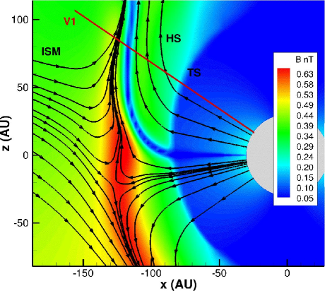
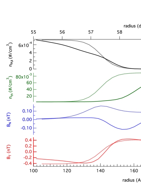
In Fig. 1, $B$ from the simulation reveals the solar wind compression at the termination shock, the downstream HS, and the HP. Profiles (solid curves in Fig. 2) along the V1 trajectory of the pick-up ($n_{\text{pui}}$) and thermal ($n_{\text{th}}$) ion densities and the azimuthal ($B_{T}$) and normal ($B_{N}$) magnetic fields near the HP are inputs for the PIC simulations. $n_{\text{pui}}$ decreases from $\approx 7\times 10^{-4}/\text{cm}^{3}$ in the HS to zero in the LISM while $n_{\text{th}}$ rises from $0.003/\text{cm}^{3}$ to $\approx 0.08/\text{cm}^{3}$. $B_{N}$ (Fig. 2C) is small at V1’s latitude in the LISM. $B_{T}$ flips direction across the HP, but remains the dominant component on both sides of the boundary (Fig. 2D). The polar angle $\delta$ (the angle between $B_{N}$ and the equatorial field) in the simulations approaches $14^{\circ}$ just outside of the HP, which is consistent with the steady values seen in the V1 data.

The MHD simulation does not match Voyager observations in several respects — the sign of the HS azimuthal magnetic field orientation, the strength of the flows in the HS and the characteristic scale length of the HP — none of which is essential for calculating initial conditions for the PIC simulations. First, because V1 continued to measure sector boundaries in the HS during 2012, and therefore probably remained in the sector zone, the sign of $B_{T}$ in the HS in the MHD model is irrelevant since a “correct” model should include the reversals associated with the sector region. Second, in contrast to the simulation, indirect measurements by the V1 LECP instrument indicate little to no normal flow in the HS (Decker et al., 2012). No published global model has explained the observed flows, although simulations that include the sectored field (e.g., Opher et al., 2012) are closer to the observations than those presented here (see also Pogorelov et al., 2012, for an alternative explanation). Finally, since the MHD model does not include the physics necessary to describe the structure of the HP, the scale length of this transition is not physical, but is instead a numerical artifact. On the other hand, what is essential for input into the PIC simulations is the strength of the HS field and the strength and orientation of the field in the LISM.

3 PIC Simulations

The initial profiles of the magnetic field, density, and temperature for the 2-D PIC simulations (dotted lines in Fig. 2; right-hand scale) were constructed with input from the MHD profiles although, in keeping with the Voyager 1 observations, there are no initial flows. The PIC code is written in normalized units based on a field strength $B_{0}$ and density $n_{0}$ (lengths normalized to the ion inertial length $d_{i}=c/\omega_{pi}$, with $\omega_{pi}$ the ion plasma frequency, times to the ion cyclotron time $\Omega_{i0}^{-1}$ and velocities to the Alfvén speed $c_{A0}$). In the HS, thermal ($n_{\text{th}}=0.25n_{0}$, $T_{\text{th}}=0.25m_{i}c_{A0}^{2}$) and pick-up ions ($n_{\text{pui}}=0.01n_{0}$, $T_{\text{pui}}=15.0m_{i}c_{A0}^{2}$) were included as independent species while the LISM only included a thermal component ($n_{\text{th}}=2.0n_{0}$, $T_{\text{th}}=0.2m_{i}c_{A0}^{2}$). The simulations were performed in a domain with dimensions $(L_{T},L_{R})=(409.6d_{i},204.8d_{i})$. The ion-to-electron mass ratio was 25 and the velocity of light was 15$c_{A0}$. Not shown in Fig. 2 are the three current sheets, of initial half-width $0.5d_{i}$, that produce the sectored HS field. This scale reflects satellite measurements at the Earth’s magnetopause that such boundaries collapse to kinetic scales (Sonnerup et al., 1981). Pressure balance across each reversal is achieved by adjusting the out-of-plane component $B_{N}$ (Smith, 2001).

For HS-appropriate values, $n=10^{-2}\text{ cm}^{-3}$ and $B=0.3\text{ nT}$, $d_{i}\approx 2\times 10^{-5}\text{ AU}$, $\Omega_{ci}^{-1}\approx 30\text{ s}$, and $c_{A}\approx 100\text{ km/s}$. Resolving kinetic scales forces the simulation domain to be much smaller than the actual system. Despite this limitation, the important physical processes can still be understood by appropriately scaling the results (Schoeffler et al., 2012).

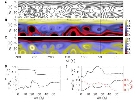
The simulations are evolved with no initially imposed perturbations. Because of the lower density, which leads to a locally higher $c_{A}$ and effectively thinner current sheets (when normalized to the local $d_{i}$), magnetic reconnection first starts in the sectored HS. Small magnetic islands grow on individual current layers in the HS and merge to become larger islands until they are comparable in size to the sector spacing (Fig. 3A). A chain of small islands grows at the HP. These merge, forming larger islands, and are compressed by HS islands pushing against the HP (Fig. 3A). By late time, the HS magnetic field has reconnected with that of the LISM, forming a complex, nested chain of islands (Fig. 3A) at the HP with sizes comparable to the original sector spacing. Along a cut from the HS to the LISM (dark line in Fig. 3A) the HP is at $\Delta R/d_{i}\sim 25$ where $B_{T}$ reverses sign (Fig. 3D). The rotation to the LISM field direction is complete by $\Delta R/d_{i}\sim 35$ after which $\delta$ and $\lambda$ are nearly constant.

We can independently track every particle in the PIC model and therefore can explore the mixing of the LISM and HS plasmas. The overall result is a highly structured distribution in the densities of the LISM ($n_{\text{LISM}}$) and HS ($n_{\text{HS}}$), with each experiencing sharp jumps across the separatrices bounding the outflows ejected from reconnection sites (Fig. 3A-C). Particles initially in the LISM continue to dominate the density on the un-reconnected LISM field lines, have mixed with HS particles in the nested islands formed from HS-LISM reconnection, and are largely excluded from islands formed from reconnection of the HS sectored field (Fig. 3B). Particles initially in the HS dominate islands resulting from reconnection of the sectored field, are mixed with LISM particles in the HP islands, and are nearly excluded from un-reconnected regions of the LISM (Fig. 3C).

Radial cuts through the simulation reveal that the increases and decreases in $n_{\text{LISM}}$ and $n_{\text{HS}}$ are typically anti-correlated (Fig. 3G). Moving from a pure HS magnetic island into an island or outflow jet where LISM and HS plasma has mixed reduces $n_{\text{HS}}$ and increases $n_{\text{LISM}}$. Along the cut the first drop in $n_{\text{HS}}$ occurs downstream of a magnetic separatrix, where HS particles have an open path to the LISM along open field lines ($\Delta R/d_{i}\sim 8$ in Fig. 3G). Similar behavior has been documented in satellite measurements at the Earth’s magnetopause (Sonnerup et al., 1981) and echoes V1’s observations of the anti-correlated variations in the fluxes of ACRs/TSPs and galactic electrons/GCRs (Stone et al., 2013; Krimigis et al., 2013; Webber & McDonald, 2013). Most important, the cuts further reveal that, when crossing the last magnetic separatrix on the LISM side of the HP before finally entering the pristine LISM plasma, the sharp decrease in $n_{\text{HS}}$ and increase in $n_{\text{LISM}}$ (in the interval $\Delta R/d_{i}=38-50$ in Fig. 3G) occur over an interval where there is no directional change in the magnetic field (Fig. 3D-E). The absence of a directional change in $\mathbf{B}$ at locations with strong variations in the particle densities is consistent with one of the most significant of the V1 observations (Burlaga et al., 2013). The fact that, in our simulation, this occurs on the LISM side of the HP therefore suggests that it may be incorrect to conclude that V1 has not crossed the HP.

The simulation cuts also reveal that local decreases in the HS density typically correspond to increases in the local magnetic field (Figs. 3F-G). The total pressure across the HP is balanced. While the dominant pressure in the HS is from the plasma, the dominant pressure in the LISM is magnetic. Thus, when reconnection opens a path for HS plasma to escape into the LISM and mix with the lower-pressure LISM plasma, there is nothing to balance the total pressure and so the region compresses to increase the magnetic field amplitude. This behavior is primarily seen at separatrix crossings remote from where reconnection locally reduces the magnetic field strength (the interval $\Delta R/d_{i}=38-50$ in Figs. 3F-G). In the V1 data, the magnetic field strength is also observed to increase where the local flux of HS plasma decreases (Stone et al., 2013; Krimigis et al., 2013; Webber & McDonald, 2013; Burlaga et al., 2013).

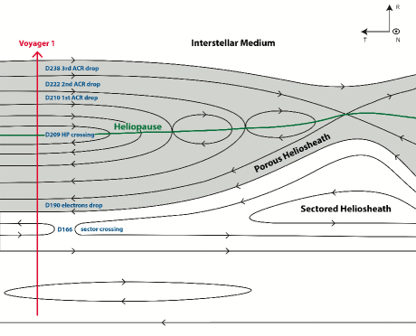
Thus, based on our simulations, we suggest that the V1 observations of simultaneous drops (increases) in HS (LISM) particle fluxes occur at a series of separatrix crossings outside of the HP that are associated with a nested set of magnetic islands that form at the HP (Fig. 4). At such crossings the magnetic field direction does not change significantly, while, as seen in the simulation data, particle fluxes can change sharply. Three active reconnection sites at the HP, and associated separatrices with two nested islands, are sufficient to explain the sequence of Voyager events. On day 166 the spacecraft crossed a current layer, on day 190 the flux of HS electrons began dropping, on day 209 another current layer was crossed and on days 210, 222 and 238 three successive drops (increases) in the HS (LISM) particle fluxes occurred. The day 190 drop in the HS electrons suggests that after this time the magnetic field was no longer laminar so that these electrons, with their small Larmor radii and large velocities, could leak into the LISM.

Islands and x-lines flowing away from an active x-line (e.g., the rightmost x-line in Fig. 4) correspond to reconnection sites that developed earlier in time. The separatrix field lines connect to x-lines, which act as bottlenecks to particle transport across the HP. There are two reasons for this. First, at the x-line the magnetic field turns into the $N$ direction since the $R$ and $T$ magnetic field components are zero. Thus, the x-line halts the field-aligned streaming of particles across the HP. Second, to the extent that $B_{N}$ is weak compared with $B_{T}$ energetic particles can scatter near x-lines, which further limits transport across the HP. In contrast, downstream of separatrices (to the left in Fig. 4) particles can freely stream across the HP. Thus, the day 210 drop in ACRs (rise in GCRs) occurred at the separatrix corresponding to the left-most x-line of Fig. 4 which blocked the transport of ACRs (GCRs) across the HP. The ACR (GCR) intensity rose (dropped) as the spacecraft crossed field lines that formed an open corridor across the HP to the left of the middle x-line in Fig. 4. In this region the flow of GCRs into the HS acts as a sink for the intensity of these particles. The second ACR drop on day 222 and subsequent recovery is similar. The final drop of the HS particle fluxes on day 238 occurred at the separatrix of the right-most x-line in Fig. 4. LECP measurements of ACR anisotropies (Krimigis et al., 2013) show that particles propagating parallel to the magnetic field dropped more rapidly than those with perpendicular pitch angles on day 238. Such behavior is consistent with our schematic – in a weakly stochastic field parallel moving particles will more quickly escape in the LISM.

An inconsistency between our PIC simulations and the observations concerns the spatial region where sharp jumps in the ACRs and GCRs take place. In the simulations the anti-correlated jumps occur on both sides of the HP but if our cartoon is correct, they occur only on the LISM side in the V1 data. The contradiction is possibly because the simulations are in a 2-D system. A magnetic field in a real 3-D system will likely be at least mildly stochastic so that wandering field lines will smooth the variability of ACR and GCR intensities far from the HP boundary. More challenging 3-D simulations will be required to explore this issue.

A second issue is the angle $\delta$ of the magnetic field outside of the HP, which for the present MHD simulation is $14^{\circ}$. $B_{ISM}$ for this simulation was chosen to match heliospheric asymmetries (Opher et al., 2009b, a). Other MHD simulations based on fitting the IBEX ribbon yield $\delta\sim 30^{\circ}$ (Pogorelov, 2013). Such values are considerably smaller than those implied by cartoons in recent publications (Burlaga et al., 2013). In any case our conclusion that significant variations in the density of the ACRs and GCRs can occur in regions with essentially no variation in the field line orientation is not sensitive to the value of $\delta$ in the LISM. Any rotation in the magnetic field outside of the HP propagates at the local Alfvén speed, which is well below the velocities of the particles of interest. Thus, outside of the HP separatrices should retain their original LISM orientation in locations where there are significant variations in particle intensity.

Combining a typical aspect ratio of reconnection-produced islands (0.1), the typical time between dropouts (10 days), and the speed of Voyager 1 with respect to the HS plasma ($\approx 20\text{ km/s}$), yields the approximate size of the islands in Fig. 4 as 1 AU. This roughly equals the sector spacing downstream of the TS and is consistent with previous simulation-derived estimates of magnetic islands in the HS (Schoeffler et al., 2012).

If the schematic with nested magnetic islands (Fig. 4) is correct, the dropouts in the HS particle fluxes occurred on the LISM side of the HP on field lines that had a LISM source. Thus, according to this picture V1 crossed the HP on day 208 and has been crossing LISM fields since that time. Our results thus suggest that $B_{T}$ in the LISM is negative (i.e., has a polarity of $270^{\circ}$).

Figure 1: A meridional cut from the global MHD simulation showing the magnetic field amplitude $B$ (background), the flow streamlines (solid curves with arrows) and the V1 trajectory (red). The HP is where the flows from the LISM and the HS meet. The blue line in the HS is the heliospheric current sheet.

Figure 2: Cuts of various parameters along the V1 trajectory near the HP from the MHD model (solid with left scale) and as initial conditions for the PIC model (dotted with right scale). Shown are in (A) the pick-up ion density, in (B) the thermal ion density, in (C) $B_{T}$ and in (D) $B_{N}$. Note that the scales on the right and left differ.

Figure 3: The structure of the HP and adjacent LISM and HS at late time. In the $R$/$T$ plane in (A) the magnetic field lines and in (B) and (C) the number density $n_{\text{LISM}}$ ($n_{\text{HS}}$) of particles that were originally in the LISM (HS), respectively. Panels (D)-(G) are cuts along the vertical line in panels (A)-(C). In (D) the azimuthal angle $\lambda$ is the angle of $\mathbf{B}$ in the $R-T$ plane with respect to the $R$ direction. In (E) the polar angle $\delta$ is the angle between $\mathbf{B}$ and the $R-T$ plane. In (F), the magnitude of B and, in (G), the number density $n_{\text{LISM}}$ (solid) and the number density $n_{\text{HS}}$ (dashed red).

Figure 4: A schematic, based on the results of our simulations, of the inferred magnetic structure of the HP during the time when V1 documented strong variations in the HS and LISM particles. The times corresponding to several of the Voyager events are marked by the days of 2012 on which they occurred.

References

- Baranov et al. (1992) Baranov, V. B., Fahr, H. J., & Ruderman, M. S. 1992, Astron. Astrophys., 261, 341
- Baranov et al. (1979) Baranov, V. B., Lebedev, M. G., & Ruderman, M. S. 1979, Astrophys. Space Sci., 66, 441
- Borovikov et al. (2011) Borovikov, S. N., Pogorelov, N. V., Burlaga, L. F., & Richardson, J. D. 2011, Astrophys. J. Lett., 728, L21
- Burlaga et al. (2005) Burlaga, L. F., Ness, N. F., Acuña, M. H., Lepping, R. P., Connerney, J. E. P., Stone, E. C., & McDonald, F. B. 2005, Science, 309, 2027
- Burlaga et al. (2013) Burlaga, L. F., Ness, N. F., & Stone, E. C. 2013, Science, published online 27 June 2013
- Decker et al. (2012) Decker, R. B., Krimigis, S. M., Roelof, E. C., & Hill, M. E. 2012, Nature, 489, 124
- Decker et al. (2005) Decker, R. B., Krimigis, S. M., Roelof, E. C., Hill, M. E., Armstrong, T. P., Gloeckler, G., Hamilton, D. C., & Lanzerotti, L. J. 2005, Science, 309, 2020
- Fahr et al. (1986) Fahr, H. J., Neutsch, W., Grzedzielski, S., Macek, W., & Ratkiewicz-Landowska, R. 1986, Space Sci. Rev., 43, 329
- Krimigis et al. (2013) Krimigis, S. M., Decker, R. B., Roelof, E. C., Hill, M. E., Armstrong, T. P., Gloeckler, G., Hamilton, D. C., & Lanzerotti, L. J. 2013, Science, published online 27 June 2013
- Liewer et al. (1996) Liewer, P. C., Karmesin, S. R., & Brackbill, J. U. 1996, J. Geophys. Res., 101, 17,119
- Opher et al. (2009a) Opher, M., Alouani Bibi, F., Toth, G., Richardson, J. D., Izmodenov, V. V., & Gombosi, T. I. 2009a, Nature, 462, 1036
- Opher et al. (2011) Opher, M., Drake, J. F., Swisdak, M., Schoeffler, K. M., Richardson, J. D., Decker, R. B., & Toth, G. 2011, Ap. J., 734
- Opher et al. (2012) Opher, M., Drake, J. F., Velli, M., Decker, R. B., & Toth, G. 2012, Ap. J., 751
- Opher et al. (2009b) Opher, M., Richardson, J. D., Toth, G., & Gombosi, T. I. 2009b, Space Sci. Rev., 143, 43
- Parker (1963) Parker, E. N. 1963, Interplanetary Dynamical Processes (New York: Interscience)
- Pogorelov (2013) Pogorelov, N. V. 2013, private communication at the ISSI Workshop on the Nature of the Heliopause in Bern, Switzerland
- Pogorelov et al. (2012) Pogorelov, N. V., Borovikov, S. N., Zank, G. P., Burlaga, L. F., Decker, R. A., & Stone, E. C. 2012, Ap. J. Lett., 750, L4
- Schoeffler et al. (2012) Schoeffler, K. M., Drake, J. F., & Swisdak, M. 2012, Ap. J. Lett., 750, L30
- Smith (2001) Smith, E. J. 2001, J. Geophys. Res., 106, 15819
- Sonnerup et al. (1981) Sonnerup, B. U. Ö., Paschmann, G., Papamastorakis, I., Sckopke, N., Haerendel, G., et al. 1981, J. Geophys. Res., 86, 10049
- Stone et al. (2005) Stone, E. C., Cummings, A. C., McDonald, F. B., Heikkila, B. C., Lal, N., & Webber, W. R. 2005, Science, 309, 2017
- Stone et al. (2013) —. 2013, Science, published online 27 June 2013
- Swisdak et al. (2010) Swisdak, M., Opher, M., Drake, J. F., & Alouani Bibi, F. 2010, Ap. J., 710, 1769
- Webber & McDonald (2013) Webber, W. R., & McDonald, F. B. 2013, Geophys. Res. Lett., accepted
- Zank et al. (1996) Zank, G. P., Pauls, H. L., Williams, L. L., & Hall, D. T. 1996, J. Geophys. Res., 101, 21,639
- Zieger et al. (2013) Zieger, B., Opher, M., Schwadron, N. A., McComas, D. J., & Toth, G. 2013, Geophys. Res. Lett., published online 21 June 2013