RMCMC: A System for Updating Bayesian Models

Abstract

A system to update estimates from a sequence of probability distributions is presented. The aim of the system is to quickly produce estimates with a user-specified bound on the Monte Carlo error. The estimates are based upon weighted samples stored in a database. The stored samples are maintained such that the accuracy of the estimates and quality of the samples is satisfactory. This maintenance involves varying the number of samples in the database and updating their weights. New samples are generated, when required, by a Markov chain Monte Carlo algorithm. The system is demonstrated using a football league model that is used to predict the end of season table. Correctness of the estimates and their accuracy is shown in a simulation using a linear Gaussian model.

Key words: Importance sampling; Markov chain Monte Carlo methods; Monte Carlo techniques; Streaming data; Sports modelling

1 Introduction

We are interested in producing estimates from a sequence of probability distributions. The aim is to quickly report these estimates with a user-specified bound on the Monte Carlo error. We assume that it is possible to use MCMC methods to draw samples from the target distributions. For example, the sequence can be the posterior distributions of parameters from a Bayesian model as additional data becomes available, with the aim of reporting the posterior means with the variance of the Monte Carlo error being less than $0.01$. We present a general system that addresses this problem.

Our system involves saving the samples produced from the MCMC sampler in a database. The samples are updated each time there is a change of sample space. The update involves weighting or transiting the samples, depending on whether the space sample changes or not. In order to control the accuracy of the estimates, the samples in the database are maintained. This maintenance involves increasing or decreasing the number of samples in the database. This maintenance also involves monitoring the quality of the samples using their effective sample size. See Table 1 for a summary of the control variables. Another feature of our system is that the MCMC sampler is paused whenever the estimate is accurate enough. The MCMC sampler can later be resumed if a more accurate estimate is required. Therefore, it may be the case that no new samples are generated for some targets. Hence the system is efficient, as it reuses samples and only generates new samples when necessary.

Our approach has similar steps to those used in sequential Monte Carlo (SMC) methods (Doucet et al., 2001; Liu, 2008), such as an update (or transition) step and re-weighting of the samples. Despite the similarities, SMC methods are unable to achieve the desired aims considered in this paper. Specifically, even though SMC methods are able to produce estimates from a sequence of distributions, it is unclear how to control the accuracy of this estimate without restarting the whole procedure. For example, consider the simulations in Gordon et al. (1993) where the bootstrap particle filter, a particular SMC method, is introduced. In these simulations the posterior mean is reported with the interval between $2.5$ and $97.5$ percentile points. As these percentile points are fixed, there is no way to reduce the length of the interval. The only hope of reducing the interval is to rerun the particle filter with more particles, although there is no guarantee. This conflicts with the aim of reporting the estimates quickly. In practice, most SMC methods are concerned with models where only one observation is revealed at a time (see simulations in e.g. Kitagawa (2014), Del Moral et al. (2006), Chopin (2002)). Our framework allows for observations to be revealed in batches of varying sizes; see the application presented in §3.

Table 1: Summary of control variables

Control Variable	Measurement	Target Interval
Accuracy of estimates ($A$)	Standard deviation of estimates	$\left[\beta_{1},\beta_{2}\right]$
Quality of samples ($Q$)	$\text{Effective sample size of database}/N_{\text{MAX}}$	$\left[\gamma_{1},\gamma_{2}\right]$

A potential application of the system is monitoring the performance of multiple hospitals where the data observed are patient records and estimate of interest relates to the quality of patient care at each hospital. Controlling the accuracy of this estimate may relate to controlling the proportion of falsely inspected hospitals. Another example of a realistic application of the system is a football league model (see §3) where the data revealed are the match results and the estimate of interest is the end of season rank league table. Controlling the estimated rank may be of interest to sports pundits and gamblers.

In §2 we define, in detail, the setup we are considering. We then describe the separate processes of the system. We also describe how to combine the weighted samples to form the estimate of interest. Then in §2.7 we present a modified batch mean approach that we use to compute the accuracy of the estimate. In §3 we investigate the performance of the system using a model for a football league. For this application, the aim is to provide quick and accurate predictions of the end of season team ranks as football match results are revealed. We examine the performance of the system as the size of data received increases. Currently, there is no theoretical proof that the proposed system is stable, however simulations verify correctness of the reported accuracy and the estimate. We present such a simulation in §4, where we apply the system using a linear Gaussian model and simulated data. We conclude in §5 with a discussion of potential future topics of research.

2 Description of the System

2.1 Setup

We now describe the settings we consider and the necessary operations required for our system to function. Let $(S_{n},\mathcal{S}_{n},\pi_{n})_{n\in\mathbb{N}}$ be a sequence of probability spaces. We are interested in reporting $\pi_{n}g_{n}=\int g_{n}(x)d\pi_{n}(x)$ where $g_{n}$ is a, possibly multivariate, random variable on $(S_{n},\mathcal{S}_{n},\pi_{n})$. In order to implement our system, the following operations are required:

1. MCMC: For all $n\in\mathbb{N}$, generate samples from an MCMC with stationary distribution $\pi_{n}$.

2. Weighting Samples: For all $k\in\overline{D}:=\{j:S_{j-1}=S_{j}\text{ and }\pi_{j}\ll\pi_{j-1}\}$, the Radon-Nikodym derivative $\frac{d\pi_{j}}{d\pi_{j-1}}$ can be evaluated.

3. Transiting Samples: For all $k\in D$ $\exists f_{k}:S_{k-1}\times[0,1]\rightarrow S_{k}$ such that $\xi\sim\pi_{k-1}$, $U\sim U[0,1]\implies f_{k}(\xi,U)\sim\pi_{k}$.

The weighting operation enables us to weight previously generated samples according to the latest measure. In the case where the sample space changes or the Radon-Nikodym derivative is not defined, the transition operation allows us to map the samples to the latest measure. If such a transition function, in operation 3, is unavailable, then the following may be used instead.

1. Transiting Samples: For all $k\in D$ $\exists f_{k}:S_{k-1}\times[0,1]\rightarrow S_{k}$.

This alternative transition operation allows us to map the samples into the latest sample space of interest.

2.2 Global Variables

The samples produced by the RMCMC process (§2.3) are stored in a database. Each sample is recorded to the database with a production date and an information cut-off. The production date is the date and time the sample was written to the database from the RMCMC process. The information cut-off refers to the measure the MCMC was targeting when the sample was produced. Lastly, each sample will be enter the database with weight $1$. The maximum number of samples allowed in the database is $N_{\text{MAX}}$. In §2.5 we explain how the control process varies $N_{\text{MAX}}$ over time. Further, we shall refer to the current number of samples in the database as $N$. The deletion process (§2.6) ensures that $N\leq N_{\text{MAX}}$ by sometimes removing samples from the database. A summary of the systems global variables is provided in Table 2 along with their descriptions.

Table 2: Description of the global variables in the rolling MCMC system.

Variable	Description
rmcmc_on	Indicator if RMCMC process is supposed to be producing new samples.
$N_{\text{MAX}}$	Maximum number of samples allowed in the database.
$N$	Number of samples contained in the database.
$(\xi_{i},w_{i})_{i=1,\dots,N}$	The samples and their corresponding weights in the database.

2.3 RMCMC Process

The RMCMC process, summarized in Algorithm 1, is an MCMC method that changes its target without the need to restart. When the target of interest changes from $\pi_{j-1}$ to $\pi_{j}$ so does the target of the MCMC. The Markov chain continues from the latest sample, making a transition step using $f_{j}$ if there is a change of sample space. This ensures the next MCMC is exploring the correct space. We continue from this sample in the hope that the Markov chain converges faster to the updated target distribution than a randomly chosen starting point. To allow the Markov chain to move toward the updated target distribution we use a burn-in period where the first $B_{0}$ samples are discarded after the target changes. This burn-in period will also weaken the dependence between samples from different target distributions. As this MCMC method is never reset and continues from the last generated sample we refer to it as a rolling MCMC (RMCMC) process.

Algorithm 1 RMCMC process

1:Parameters: MCMC algorithm, $B_{0}$.

2:repeat indefinitely.

3:     if target changes to $\pi_{j}$ then

4:         Set $B=B_{0}$.

5:         Update target of MCMC to $\pi_{j}$.

6:         if $j\in D$ then

7:              Set current position of MCMC to $f_{j}(\xi,U)$ where $U\sim U[0,1]$ and $\xi$ is the latest sample generated.               

8:     if rmcmc_on=true then

9:         Perform MCMC step.

10:         if $B=0$ then write sample to database with weight $1$.

11:         else $B\leftarrow B-1$.          

12:     else sleep for some time.      

The RMCMC process is only active when new samples are required as it can be paused and resumed by the control process (§2.5). If the process is paused for long periods, it may be the case that no samples are produced for some targets. In Algorithm 1 the generated samples are written to the database individually. In practice, however, it may be more convenient to write the samples to the database in batches. This practice is allowable and will not affect the functioning of the system.

2.4 Update Process

The update process, presented in Algorithm 2, ensures that the samples are weighted correctly each time the target changes. There are two types of updates depending on the measures and their sample spaces. More precisely, consider a change of target from $\pi_{j-1}$ to $\pi_{j}$. If $j\in D$, that is the sample spaces differ or the Radon-Nikodym $d\pi_{j}/d\pi_{j-1}$ is not defined, then the function $f_{k}$ is used to map the samples in the database onto the new space. On the other hand, if $j\notin D$, the samples are first re-weighted according to $d\pi_{j}/d\pi_{j-1}$, then scaled. We now discuss this re-weight and scaling steps in more detail.

Suppose that the RMCMC process produces the samples $\xi_{1},\dots,\xi_{m}\sim\pi_{j-1}$ where $\pi_{j-1}$ is the target of interest. Next, suppose the the target changes from $\pi_{j-1}$ to $\pi_{j}$. In order to use the samples from the previous measure, $\pi_{j-1}$, for estimating $\pi_{j}g_{j}$, the weights are updated as follows. For $i=1,\dots,m$ define the updated weight $W_{i}$ from $w_{i}$ as

$$W_{i}=w_{i}v_{i}\quad\text{where}\quad v_{i}\propto\frac{d\pi_{j}}{d\pi_{j-1}}(\xi_{i}).$$

After, the weights are scaled such that the sum of the weights is equal to their effective sample size. More precisely, define the scaled weight $\widehat{w}_{i}$ from $W_{i}$ as

$$\widehat{w}_{i}=W_{i}\frac{\sum_{k=1}^{m}W_{k}}{\sum_{k=1}^{m}W_{k}^{2}}\quad(i=1,\dots,m).$$

Straightforward calculations show that scaling in this fashion ensures the effective sample size of the database is the sum of the effective sample sizes of the most recently weighted samples and the newly generated samples.

Algorithm 2 Update Process

1:repeat indefinitely.

2:     if the target changes from $\pi_{j-1}$ to $\pi_{j}$ then

3:         Label the out-of-date samples $\xi_{1},\dots\xi_{m}$ with corresponding weights $w_{1},\dots,w_{m}$.

4:         if $j\notin D$ then

5:              Update the weight $w_{i}\leftarrow w_{i}v_{i}$ where $v_{i}\propto\frac{d\pi_{j}}{d\pi_{j-1}}(\xi_{i})$ for $i=1,\dots,m$.

6:              Compute $d=\left(\sum_{k=1}^{m}w_{k}\right)/\left(\sum_{k=1}^{m}w_{k}^{2}\right)$.

7:              Set $w_{i}\leftarrow dw_{i}$ for $i=1,\dots,m$.

8:              Write the weights into the sample database.          

9:         if $j\in D$ then

10:              Replace samples by $f_{j}(\xi_{i},U_{1}),\dots,f_{j}(\xi_{m},U_{m})$ where $U_{1},\dots,U_{m}\stackrel{{\scriptstyle\text{iid}}}{{\sim}}U[0,1]$, leaving the weights unchanged.          

11:     else sleep for some time.      

2.5 Control Process

The control process determines when the RMCMC process is paused and changes the maximum number of samples contained in the database. This is done to maintain the accuracy of the estimate of interest and the quality of the samples. We now discuss each of these in turn.

At any given time, denote the samples in the database by $\xi_{1},\dots,\xi_{N}$. For $i=1,\dots,N$ denote the $i$th sample weight in the database as $w_{i}$. To estimate the quantity of interest $\pi_{k}g_{k}$, for some $k\in\mathbb{N}$, we use the estimator

$$T=\frac{\sum_{i=1}^{N}w_{i}g_{k}(\xi_{i})}{\sum_{i=1}^{N}w_{i}}.$$

The accuracy of the estimate, $A$, is defined as the standard deviation of $T$ (in §2.7 we discuss how to estimate $A$). The process aims to control the accuracy $A$ such that $A<\epsilon$ for some fixed $\epsilon>0$. When considering multiple estimates i.e. multivariate $g_{k}$, we force the standard deviation of all the estimates below the threshold $\epsilon$. One approach to control the accuracy would be to pause the RMCMC process each time $A<\epsilon$ and resumed if $A\geq\epsilon$. However, this may lead to the RMCMC process being paused and resumed each time a new observation is revealed, as a small change in the accuracy will inevitably occur. Therefore, we use $0<\beta_{1}<\beta_{2}\leq\epsilon$ so that if $A\leq\beta_{1}$ the RMCMC process is paused and if $A>\beta_{2}$ the RMCMC process is resumed.

The control process is also controls the quality of the samples in the database. The process aims to hold a good mixture of samples in the hope that a future change of measure does not require the resuming of the RMCMC process. We define the quality of the samples in the database as

$$Q=\frac{\text{ESS}}{N_{\text{MAX}}}\quad\text{where}\quad\text{ESS}=\frac{\left(\sum_{i=1}^{N}w_{i}\right)^{2}}{\sum_{i=1}^{N}w_{i}^{2}}.$$

The quality of the samples, $Q$, is the effective sample size of the all the weights in the database divided by the optimal effective sample size of the database, $N_{\text{MAX}}$. The optimal effective size of the database consists of a database with $N_{\text{MAX}}$ samples all with weight 1. As with the accuracy, we aim to maintain the quality such that $\gamma_{1}<Q<\gamma_{2}$ for some $0<\gamma_{1}<\gamma_{2}\leq 1$. The control process is summarised in Algorithm 3. To ensure that the database in never depleted, a minimum number of samples is imposed at $N_{\text{MIN}}>0$ such that the number of samples, $N$ and $N_{\text{MAX}}$ cannot drop below $N_{\text{MIN}}$. Therefore, when the RMCMC process is paused, $Q<\gamma_{1}$ and $N_{\text{MAX}}=N_{\text{MIN}}$ we cannot decrease $N_{\text{MAX}}$ any more. In this case, the RMCMC process is resumed to generate new samples that replace the poor quality samples in the database.

Algorithm 3 Control Process

1:Parameters: $\beta_{1},\beta_{2},\gamma_{1},\gamma_{2},N_{\text{MIN}}$.

2:repeat indefinitely.

3:     Compute $Q$ and $A$.

4:     if $A<\beta_{1}$ and $N\geq N_{\text{MIN}}$ then set rmcmc_on=false.      

5:     if ($A>\beta_{2}$) or (rmcmc_on=false and $Q<\gamma_{1}$ and $N=N_{\text{MIN}}$) then set rmcmc_on=true      

6:     if rmcmc_on=false and $Q<\gamma_{1}$ and $N>N_{\text{MIN}}$ then decrease $N_{\text{MAX}}$.      

7:     if rmcmc_on=true and $Q>\gamma_{2}$ then increase $N_{\text{MAX}}$.      

2.6 Deletion Process

This process deletes samples from the database if the current number of samples, $N$, exceeds the maximum number of samples allowed $N_{\text{MAX}}$. Removing samples from the database reduces the computational work performed by the update process and calculating the estimates. Moreover, lowering the number of samples is the way the control process maintains the quality of the samples. For simplicity, if $N>N_{\text{MAX}}$, the $N-N_{\text{MAX}}$ samples that were produced the earliest are removed. The deletion process is summarized in Algorithm 4.

Algorithm 4 Deletion Process

1:repeat indefinitely.

2:     if $N>N_{\text{MAX}}$ then delete samples from the database.

3:     else sleep for some time.      

2.7 Modifying Batch Means to Estimate the Accuracy

There are several methods to estimate the variance of MCMCs such as block bootstrapping (Lahiri, 2003, Chapter 3), batch means (Flegal and Jones, 2010) and initial sequence estimators (Geyer, 1992). In our system the samples in the database have weights which complicates estimation of the variance. The aforementioned methods cannot be used as they essentially treat all samples with equal weight. We now present a version of the batch mean approach that is modified to account for the sample weights.

Assume the estimate of interest is $\pi_{n}g_{n}$ for some $n\in\mathbb{N}$. First, order the samples in the database $\xi_{1},\dots,\xi_{N}$ and their corresponding weights $w_{1},\dots,w_{N}$ by their production date. This ensures that the dependence structure of the samples is maintained. Then we divide the samples into batches or intervals of length $b$ according to their weights. More precisely, let $D_{0}=0$, $D_{j}=\sum_{i=1}^{j}w_{i}$ and $L=\lceil\sum_{i=1}^{N}w_{i}/b\rceil$ be the number of batches. It may be the case that a weight spans more than one interval. Therefore we need to divide each weight by the proportion it spans a given interval. For the $i$th interval and $u$th sample define $\kappa_{i}(u)=\left[\min\left\{D_{u},ib\right\}-\max\left\{D_{u-1},(i-1)b\right\}\right]^{+}$, where $\left[x\right]^{+}=\max\left(0,x\right)$, for $i=1,\dots,L$. Then $\kappa_{i}(u)$ is the batch weight of $\xi_{u}$ in interval $i$. The mean of the weighted samples in the $i$th interval is

$$\widehat{\mu}_{i}=\frac{\sum_{u=1}^{N}\kappa_{i}(u)g_{n}(\xi_{u})}{\sum_{u=1}^{N}\kappa_{i}(u)}.$$

Finally, we estimate the squared accuracy by

$$\hat{A}^{2}=\frac{1}{L}\sum_{i=1}^{L}\left(\widehat{\mu}_{i}-\widehat{\mu}\right)^{2},\quad\widehat{\mu}=\frac{1}{L}\sum_{j=1}^{L}\widehat{\mu}_{j}\text{ }.$$

The batch length $b$ should be large enough to capture the correlation between samples, yet small enough to give a stable estimate of the variance. In practice we recommend using several batch lengths in order to get a conservative estimate of $A$. Moreover, the batch mean estimate should not be trusted when the number of batches, $L$, is low. This can occur as $\sum_{i=1}^{N}w_{i}$ can become very small. In this case, we suggest setting the accuracy $A$ to $-1$ nominally. This prompts the control process to remove samples from the database and then restart the RMCMC process. This action effectively replenishes the database with new samples. In practice, we recommend taking this action when $L<20$.

2.8 Remarks

2.8.1 Effective sample size for correlated samples.

The quality, $Q$, uses the effective sample size defined for independent samples, not correlated samples which we use in our system. In the system, consider the extreme case where all samples have the same value i.e. $\xi_{1}=\dots=\xi_{N}$ produced from the same target. Each of these samples will have the same weight and therefore $Q=1$ suggesting the optimal quality has been achieved. Further, the accuracy of the estimate, $A$, will be very low since the weights and samples are all the same. Hence, in this extreme case, the control process would take no action. This is clearly undesirable. Ideally, the effective sample size used to calculate $Q$, should take into account the autocorrelation of the samples, where high autocorrelation (in absolute value) leads to a lower effective sample size. However, we use the this version the effective sample size for independent samples as it is quick and simple to compute.

2.8.2 Degeneracy of the Sample Weights.

We now discuss how the system handles two types of degeneracy of the sample weights. The first is where a single sample in the database has most of the total weight and all other samples have $0$ or nearly $0$ weight. If this were to occur, the effective sample size, and therefore the quality, $Q$, will be very low. In this case, the control process will remove samples from the database before resuming the RMCMC process. The second is where all sample weights are $0$ or nearly $0$. As a consequence, the sum of the weights, $\sum_{i=1}^{N}w_{i}$, will be very low. Recall that the batch mean approach uses $L=\lceil\sum_{i=1}^{N}w_{i}/b\rceil$ batches where $b$ is the length of the batch. Further, if $L<20$ the control process removes samples from the database and resumes the RMCMC process. Therefore, in the case where $\sum_{i=1}^{N}w_{i}$ drops to low, the sample database in replenished. To summarise, the system does not attempt to avoid these types of degeneracy, but to take remedial action when it does occur.

2.8.3 Burn-in Periods.

In the RMCMC process, we perform a burn-in each time a change of measure occurs. In some cases, however, it may not be necessary, as we now discuss. Assume we have the samples $\xi_{1},\dots,\xi_{m}\sim\pi_{j-1}$. Next, consider a change of measure from $\pi_{j-1}$ to $\pi_{j}$ such that $j\in D$. In this case, a burn-in period is unnecessary as the new chain starts at a representative of $\pi_{j}$, namely $f_{j}(\xi_{m},U)\sim\pi_{j}$ where $U\sim U[0,1]$. On the other hand, if either the samples $\xi_{1},\dots,\xi_{m}$ are not from $\pi_{j-1}$ or the transition function in operation $3^{\prime}$, but not operation $3$, is available, then a burn-in period is required. In any case, performing a burn-in is mostly harmless.

2.8.4 Subsampling.

The samples produced from a MCMC method are correlated. If the correlation of the samples is high then a large number of samples are required to achieved the desired accuracy of the estimate. As a consequence, the update process and the calculation of the estimate would take a long time. To alleviate this problem we use subsampling.

Use of subsampling within an MCMC method entails saving only some samples produced. More precisely, with a subsampling size $k$, every $k$th sample is saved and the rest discarded. To choose the subsampling size $k$, we suggest performing a pre-initialisation run of the MCMC on the initial set of data. One approach, that we use in our implementation of the system, is to vary $k$ until $\rho:=\varsigma^{2}/\text{var}\left\{g_{1}(\xi_{1})\right\}\approx 2$ where $\varsigma^{2}=\text{var}\left\{g_{1}(\xi_{1})\right\}+2\sum_{j=1}^{\infty}\text{cov}\left\{g_{1}(\xi_{1}),g_{1}(\xi_{1+j})\right\}$. We found that setting $\rho\approx 2$ worked well in our implementations of the system, however may not be appropriate in all applications. In practice, a method such as initial sequence methods (Geyer, 1992) or a batch mean approach (Brooks et al., 2011, §1.10.1) can be used to estimate $\varsigma^{2}$. We chose to use the batch mean approach in our system.

If the initial Markov chain $\xi_{1},\xi_{2},\dots$ is Harris recurrent and stationary with invariant distribution $\pi$, then by the Markov chain central limit theorem (e.g. Jones, 2004)

$$\sqrt{n}\left\{\frac{1}{n}\sum_{i=1}^{n}g(\xi_{i})-\int g(x)\pi(dx)\right\}\xrightarrow[]{d}N\left(0,\varsigma^{2}\right)\quad\text{as}\quad n\rightarrow\infty.$$

Thus $\varsigma^{2}$ is the asymptotic variance of the Markov chain. Hence, by choosing $\rho\approx 2$, we obtain

$$2\sum_{j=1}^{\infty}\text{cov}\left\{g(\xi_{1}),g(\xi_{1+j})\right\}\approx\text{var}\left\{g(\xi_{1})\right\}$$

i.e. the sum of all covariance terms contributes as much as $\text{var}\left\{g(\xi_{1})\right\}$ to $\varsigma^{2}$. This way, the covariance between the samples is prevented from getting to large relative to $\text{var}\left\{g(\xi_{1})\right\}$.

2.8.5 Choice of Scaling.

As discussed in §2.3, the database will consist of weighted samples from different target distributions. In §2.5 the weighted sample average, $T$, is used to estimate $\pi_{j}g_{j}$ for some $j\in\mathbb{N}$. In this subsection we show that, due to the scaling of the weights (§2.4), the variance of $T$ is minimised under certain assumptions. A similar calculation can be found in Gramacy et al. (2010).

We begin by showing that $T$ can be decomposed according to two sets of samples. Denote the invariant measure of the RMCMC process at a given time instance as $\pi_{j}$ for some known $j\in\mathbb{N}$. Further, label the samples produced from this MCMC targeting $\pi_{j}$ as $\xi_{m+1},\dots,\xi_{N}$ for some $m\in\{0,\dots,N\}$. The case $m=N$ corresponds to the situation when no samples have been produced from $\pi_{j}$. Label the remaining sample as $\xi_{1},\dots,\xi_{m}$. These samples will have already been weighted and scaled in previous iterations.

The estimator, $T$, can be decomposed according to the two sets of samples as

$$T=\frac{\sum_{i=1}^{m}\widehat{w}_{i}g_{j}(\xi_{i})+\sum_{i=m+1}^{N}g_{j}(\xi_{i})}{\sum_{i=1}^{m}\widehat{w}_{i}+(N-m)}$$

as $w_{j}=1$ for $j=m+1,\dots,N$. In terms of the updated weights, $T$ can be written as $T=\alpha T_{1}+(1-\alpha)T_{2}$ where $T_{1}=\sum_{i=1}^{m}W_{i}g_{j}(\xi_{i})/\sum_{i=1}^{m}W_{i}$ and $T_{2}=\sum_{i=m+1}^{N}g_{j}(\xi_{i})/(N-m)$ are the individual estimators of $\pi_{j}g_{j}$ given by the two sets of samples and

$$\alpha=\frac{\text{ESS}_{m}}{\text{ESS}_{m}+(N-m)}\quad\text{where}\quad\text{ESS}_{m}=\frac{\left(\sum_{i=1}^{m}W_{i}\right)^{2}}{\sum_{i=1}^{m}W_{i}^{2}}.$$

The choice of the scaling performed in the update process (§2.4) led to this choice of $\alpha$. We now show that this choice of $\alpha$, under certain assumptions, minimises the variance of $T$. Assume $\phi\in\mathbb{R}$ is a constant. Then the variance of the estimator $T=\phi T_{1}+(1-\phi)T_{2}$ is $\text{var}(T)=\phi^{2}\text{var}(T_{1})+(1-\phi)^{2}\text{var}(T_{2})$ where we assume that $T_{1}$ and $T_{2}$, or more specifically the two sets of samples $\xi_{1},\dots,\xi_{m}$ and $\xi_{m+1},\dots,\xi_{N}$, are independent. The variances of the individual estimators are

$$\text{var}(T_{1})=\frac{\sigma^{2}}{\text{ESS}_{m}}\quad\text{and}\quad\text{var}(T_{2})=\frac{\sigma^{2}}{N-m}$$

where we assume $\text{var}\left\{g_{j}(\xi_{i})\right\}=\sigma^{2}$, for $i=1,\dots,N$ and that the weights are constants. Upon differentiating we find that setting $\phi$ to $\text{ESS}_{m}/\{\text{ESS}_{m}+(N-m)\}$ minimises $\text{var}(T)$ thus regaining $\alpha$. These assumptions are unrealistic in our setting. However, this motivates the use of a burn-in period within the RMCMC process after new data are observed. Although we can not guarantee independence between the sets of samples, the burn-in period at least weakens their dependence.

3 Application to a Model of a Football League

In this section we demonstrate how the system performs on a model of a football league. The data we use are the English Premier League results from $2005/06$ to $2012/13$ season. In a season, a team plays all other teams twice. For each match played, a team receives points based on the number of goals they and their opponent scores. If a team scores more goals than their opponent they receive $3$ points. If a team score the same number of goals as their opponent they receive $1$ point. If a team scores less goals than their opponent they receive $0$ points. The rank of each team is determined by their total number of points, where the team with the highest number of points is ranked $1$st. A tie of ranks then determined by goal difference and then number of goals scored.

We are interested in the probability of each rank position for all teams at the end of a season. The aim is to estimate these rank probabilities to a given accuracy. Thus, in this application we are concerned about maintaining the accuracy of multiple predictions.

Throughout this section, we use the following notation. Let $I_{p}$ be the $p\times p$ identity matrix and $1_{p}$ be a vector of $1$s of length $p$. Further, let $\text{N}(\mu,\Sigma)$ denote a multivariate normal distribution with mean $\mu$ and covariance matrix $\Sigma$. Denote the cardinality of a set $A$ by $\left|A\right|$. We shall reserve the index $t=1,\dots,T$ for reference to seasons. Lastly, let $\text{logN}(\mu,\sigma^{2})$ denote a log-normal distribution i.e. if $X\sim\text{N}(\mu,\sigma^{2})$ then $\exp(X)\sim\text{logN}(\mu,\sigma^{2})$.

We begin by presenting a model for football game outcomes. The model we use is similar to that presented in Glickman and Stern (1998) and Dixon and Coles (1997).

3.1 Football League Model

Consider a model with hidden Markov process $X_{t}$ ($t\in\mathbb{N}$), observed process $Y_{t}$ ($t\in\mathbb{N}$) and parameter $\theta$. The observation $Y_{t}$ contains all observations for state $X_{t}$. Denote the $j$th observation of state $t$ as $Y_{j,t}$. Next define the $k$th observation batch of state $t$ as $\widetilde{Y}_{k,t}$ for $k=1,\dots,c_{t}$ for some $c_{t}\geq 1$. For instance, if the observations are batched in groups of $10$, the $k$th batch of state $t$ is $\widetilde{Y}_{k,t}=Y_{10k-9,t},\dots,Y_{10k,t}$. In this application section, we are interested in the model

$$\begin{cases}p(x_{t}|x_{1:t-1},\theta)=p(x_{t}|x_{t-1},\theta)\\ p(\widetilde{y}_{k,t}|\widetilde{y}_{1:(k-1),t},y_{1:(t-1)},x_{1:t},\theta)=p(\widetilde{y}_{k,t}|x_{t},\theta)\\ p(x_{1}|\theta),p(\theta)\end{cases}.$$ (1)

where $\widetilde{y}_{1:0,t}$ is an empty observation batch introduced for notational convenience. In this section, the sequence of target distributions is defined as follows. Let $\varpi_{k,t}=p(x_{1:t},\theta|\widetilde{y}_{1:k,t},y_{1:(t-1)})$ for $t=1,2,\dots$ and $k=0,\dots,c_{t}$. Then, we are interested in the targets $\pi_{n}=\varpi_{\varphi_{1}(n),\varphi_{2}(n)}$ for $n\in\mathbb{N}$ where

$$\varphi_{2}(n)=\max\left\{j\in\mathbb{N}:(n-1)\geq\sum_{i=1}^{j-1}(c_{i}+1)\right\},\quad\varphi_{1}(n)=n-1-\sum_{i=1}^{\varphi_{2}(n)-1}(c_{i}+1),$$

where we set $\sum_{i=1}^{0}(c_{i}+1)=0$. The transition steps occur at $k\in D=\{n\in\mathbb{N}:\varphi_{1}(n)=0\}$. In this application, the transition functions $f_{k}$ ($k\in D$) are dictated by the model namely $p(x_{t}|x_{t-1},\theta)$ in (1).

We now describe the states $X_{t}$, the observations $Y_{t}$ and the parameter $\theta$ in this football application. Each team is assumed to have a strength value (in $\mathbb{R}$) which remains constant within a season. Let $U_{t}$ be the set of teams that play in season $t$, $X_{i,t}$ be the strength of team $i$ in season $t$ and $X_{t}=(X_{i,t})_{i\in U_{t}}$. To condense notation, for any set $A\subset U_{t}$ define $X_{A,t}:=(X_{i,t})_{i\in A}$ and form the parameter vector $\theta=(\lambda_{H},\lambda_{A},\sigma_{p},\sigma_{s},\eta,\mu_{p})$, which we now define.

At the end of every season, some teams are relegated and new teams are promoted to the league. Denote the set of promoted teams that begin season $t$ by $W_{t}$ and let $V_{t}=U_{t}\backslash W_{t}$ be the set of teams that remain in the league from season $t-1$ to $t$. The promoted teams strengths are introduced such that $X_{W_{t},t}|(\theta,X_{t-1}=x_{t-1})\sim\text{N}\left(\mu_{p}1_{\left|W_{t}\right|},\sigma_{p}^{2}I_{\left|W_{t}\right|}\right)$. Thus any previous history in the league is not used for a promoted team. From season $t-1$ to $t$, the strengths of the teams that were not relegated are evolved such that $X_{V_{t},t}|(\theta,X_{t-1}=x_{t-1})\sim\text{N}\left(\eta C_{t}x_{V_{t},t-1},\sigma_{s}^{2}I_{\left|V_{t}\right|}\right)$. Thus between seasons, the strengths of the teams that are not relegated are centered around $0$ and expanded ($\eta>1$) or contracted ($\eta<1$). Next, consider a match, in season $t$, between home team $j$ and away team $k$ ($j,k\in U_{t}$). We assume the number of home $G_{j,H}^{k}$ and away goals $G_{k,A}^{j}$ is modelled by $G_{j,H}^{k}|(\theta,X_{t})\sim\text{Poisson}\left(\lambda_{H}\exp\left\{x_{j,t}-x_{k,t}\right\}\right)$ and $G_{k,A}^{j}|(\theta,X_{t})\sim\text{Poisson}\left(\lambda_{A}\exp\left\{x_{k,t}-x_{j,t}\right\}\right)$ independently of each other. The parameters $\lambda_{H}$ and $\lambda_{A}$ are strictly positive and pertain to the home and away advantage (or disadvantage) which is assumed to be the same across all teams and all seasons. More precisely, $\lambda_{H}$ ($\lambda_{A}$) is the expected number of home (away) goals in a match between two teams of equal strength. Finally, denote the results of season $t$ by $Y_{t}$; the number of home and away goals for all games in season $t$. For this football application, the sample space is $S_{n}=\mathbb{R}^{20\varphi_{2}(n)+2}\times(\mathbb{R}^{+})^{4}$.

For the first season strengths, we use an improper flat prior. For the home and away advantage we take respective Gamma distribution priors of shapes $5$ and $2$ and scales $5$ and $1$. For $(\eta,\sigma_{s})$ and $(\mu_{p},\sigma_{p})$ we take their Jeffreys priors. Jeffreys prior was used for both $(\eta,\sigma_{s})$ and $(\mu_{p},\sigma_{p})$ after considering the amount of information available for each parameter. For instance, if 10 seasons are considered, only 9 transitions between seasons are available for the likelihood of $(\eta,\sigma_{s})$. Thus, using an informative prior would greatly influence the posterior distribution. This can also be argued for the promotion parameters $(\mu_{p},\sigma_{p})$.

3.2 The MCMC Step

For the MCMC step in the RMCMC process (Algorithm 1), we use a Metropolis-Hasting algorithm (Metropolis et al., 1953), (Hastings, 1970). In general, a different, potentially more complex MCMC method can be used. However, the system does not rely on the choice of MCMC method, and will work with a simple sampler, as demonstrated in this application. We use independent proposal densities for the separate parameters. Due to the high dimension of the combine states and parameter, we choose to implement block updates (Brooks et al., 2011, Section 21.3.2). This entails proposing parts of the state and parameter at any stage. The proposals densities used and the block updating is summarized in Algorithm 1. In the algorithm we propose a new strength of a single season $80$% of the time and part of the parameter $\theta$ the remaining $20$%. This was done so that exploration of the chain was mainly focused on the states. The proposal densities parameters were determined by consideration of the acceptance rate in a pre-initialization run of the MCMC. Lastly, the samples were written into the database in batches of $1,000$.

Algorithm 1 Block Proposals for Metropolis-Hasting Algorithm

1:Given $(x_{1:t},\lambda_{H},\lambda_{A},\eta,\sigma_{s},\mu_{p},\sigma_{p})$.

2:Generate $u\sim\text{Uniform}(0,1)$.

3:if $u<0.8$ then

4:     Generate $v\sim\text{Uniform}\{1,\dots,t\}$.

5:     Propose $x_{v}^{*}|x_{v}\sim\text{N}(x_{v},0.0002I_{\left|U_{v}\right|})$

6:if $u\geq 0.8$ then Generate $w\sim\text{Uniform}\{1,\dots,4\}$.

7:     if $w=1$ then propose $\lambda_{H}^{*}|\lambda_{H}\sim\text{logN}(\log(\lambda_{H}),0.01^{2})$.      

8:     if $w=2$ then propose $\lambda_{A}^{*}|\lambda_{A}\sim\text{logN}(\log(\lambda_{A}),0.01^{2})$.      

9:     if $w=3$ then propose $\eta^{*}|\eta\sim\text{N}(\eta,0.01)$ and $\sigma_{s}^{*}|\sigma_{s}\sim\text{logN}(\log(\sigma_{s}),0.005)$.      

10:     if $w=4$ then propose $\mu_{p}^{*}|\mu_{p}\sim\text{N}(\mu_{p},0.0002)$ and $\sigma_{p}^{*}|\sigma_{p}\sim\text{logN}(\log(\sigma_{p}),0.002)$.      

3.3 League Predictions

In §3.1 we introduced a model for the team strengths and the outcome of football matches, in terms of goals scored. In §3.2 we presented the MCMC method which produces samples used to estimate the states and parameters of the model. We now explain how these samples are used to predict the end of season ranks of each team, which is our estimates of interest i.e. $\pi_{n}g_{n}$.

For each sample, all games in a season are simulated once. Thus each sample gives a predicted end of season rank table. The distribution across these predicted rank tables gives the estimated probabilities of the ranks of each team. This distribution is the posterior summary of interest whose accuracy we aim to control.

3.4 System Parameters

As mentioned in §2.8, we performed a pre-initialization run using $10,000$ samples to determine the subsampling size. Based on the results from the 2005/06 to the 2009/10 season, we found that a subsample size of $80$ gave $\varsigma\approx 2$. We used a burn-in period of $B_{0}=10,000$ within the RMCMC process. Within the control process we use $\beta_{1}=0.01$ and $\beta_{2}=0.0125$ for the accuracy thresholds and $\gamma_{1}=0.1$ and $\gamma_{2}=0.75$ for the quality thresholds. Whenever the control process demanded a change in $N_{\text{MAX}}$, it was increased or decreased by $10$% of its current value. Finally, we set $N_{\text{MIN}}=1,000$.

As mentioned in §3.3, our estimate consists of rank probabilities for each team i.e. each team has estimated probabilities for ending the season ranked $1\text{st},\dots,20\text{th}$. The accuracy of each of the $400$ rank probabilities is calculated using the method presented in §2.7 using use two batch lengths $b=10$ and $b=50$. The maximum standard deviation is reported as the accuracy of the estimate to be conservative.

3.5 Results

The system is initialized with the results from the 2005/06 to 2009/10 seasons of the English Premier League. Using the samples from this initialisation, we proceeded with $3$ separate runs of the system. The system itself remained unchanged in each of the runs, however, the way the results for the next $2$ seasons were revealed varied. The match results were revealed individually, in batches of $7$ days and in batches of $30$ days. New data batch were revealed only if the RMCMC process was paused.

In Table 3 we present the system results of each run. We see that for larger data batches, the RMCMC process is resumed more often. Further, the percentage of new samples generated after new data are revealed increases as with the size of the data batch. The average percentage of new samples is calculated as follows. Before a new data batch is revealed the percentage of new samples in the database generated after the introduction of the latest data is calculated. The average of these percentages is then taken over the data batches. This means that for larger data batches the RMCMC process will often be resumed to generate new samples that replace most of the samples already in the database.

Table 3: System summary for various data batch sizes.

	individual	7 day	30 day
No. of batches	760	70	20
Range of games per batch	[1,1]	[3,21]	[10,53]
No. times RMCMC resumed	39	31	18
Total No. MCMC steps	24,010,000	14,230,000	9,240,000
Average % of new samples	2%	20%	53.6%

In Table 4 we present the estimated posterior mean of the components of $\theta$ at the end of the run for each batch size. As expected, being based on the same data, these final estimates are almost identical for the various batch sizes. In Table 5 we present the predicted end of 2012/13 season ranks for selected teams and ranks. Each team and rank has $3$ predictions given by the runs using different batch sizes. For each batch size, these predictions are being controlled. More precisely, for every rank of every team the predictions standard deviation is being controlled below $\beta_{2}=0.0125$. This is consistent with the predictions across the various batch sizes. The predictions for all teams and ranks can be found in §A in the Appendix.

Table 4: End of run parameter estimated mean with $95$% credible intervals.

Parameter	individual	7 day	30 day
$\lambda_{H}$	1.446 (1.406,1.497)	1.447 (1.406,1.496)	1.446 (1.406,1.494)
$\lambda_{A}$	1.031 (0.998,1.073)	1.032 (0.995,1.073)	1.032 (0.997,1.077)
$\eta$	0.970 (0.865,1.054)	0.967 (0.865,1.049)	0.964 (0.864,1.048)
$\sigma_{s}$	0.083 (0.061,0.117)	0.084 (0.059,0.113)	0.086 (0.059,0.116)
$-\mu_{p}$	0.245 (0.316,0.172)	0.242 (0.322,0.167)	0.244 (0.315,0.171)
$\sigma_{p}$	0.116 (0.049,0.204)	0.117 (0.063,0.191)	0.114 (0.06,0.202)

Table 5: End of 2012/13 season rank predictions for selected teams and ranks. Each team and rank has $3$ predictions given by (from top to bottom) the individual, $7$ day and $30$ day batch run.

	Rank
Team	1	2	3	$\dots$	18	19
Arsenal	8%	14%	17%	$\dots$	0%	0%
	8%	14%	17%	$\dots$	0%	0%
	8%	15%	19%	$\dots$	0%	0%
Aston Villa	0%	0%	1%	$\dots$	6%	5%
	0%	0%	1%	$\dots$	6%	5%
	0%	0%	1%	$\dots$	6%	5%
Chelsea	9%	15%	19%	$\dots$	0%	0%
	9%	15%	21%	$\dots$	0%	0%
	10%	16%	20%	$\dots$	0%	0%
Everton	1%	2%	6%	$\dots$	1%	1%
	1%	3%	5%	$\dots$	1%	1%
	1%	2%	5%	$\dots$	1%	1%
⋮	⋮	⋮	⋮	⋮	⋮	⋮
Wigan	0%	0%	0%	$\dots$	10%	11%
	0%	0%	0%	$\dots$	10%	11%
	0%	0%	0%	$\dots$	11%	12%

In the following, we present some results for the $7$ day batch run only. Further results for all the batch sizes are presented in §A in the Appendix. In Figure 1 we display the accuracy of the predictions ($A$), the quality of the samples ($Q$) and the number of samples in the database ($N$) as new data are revealed. In Figure 1a, the control process attempts to keep the accuracy of the predictions between $\beta_{1}=0.01$ and $\beta_{2}=0.0125$. Occasionally, after new data are revealed, the accuracy exceeds the upper threshold $\beta_{1}$. The accuracy drops nominally to $0$ at the end of each season prior to the introduction of the next seasons fixtures. Similarly, in Figure 1b, the quality of the samples is attempted to be kept between $\gamma_{1}=0.1$ and $\gamma_{2}=0.75$. In Figure 1c, we see that the number of samples in the database, $N$, varies over time. More precisely, after $5$ batches of data, $19,246$ samples are used. However, later the number of samples used decreases to approximate $14,000$ samples. Similar features are seen for the different batch sizes. The change in the accuracy of the predictions and the quality of the samples gets smaller as the batch size decreases.

Figure 1d is a plot of the Kaplan-Meier estimator (Kaplan and Meier, 1958) of the survival function of the samples in the database as new data are revealed. More precisely, let $U$ be a random variable of the number of new data batches observed before a sample is deleted. Then Fig 1d is a plot of the Kaplan-Meier estimator of $S(u)=P(U>u)$. The Kaplan-Meier estimator takes into consideration the right-censoring due to the end of the simulation i.e. samples that could have survived longer after the simulation ended. We see that samples survive as new data are observed e.g. a sample survives $10$ or more batches with probability $0.33$. Thus samples are reused as envisaged in §2.4. Lastly, from using the different batch sizes (see §A in the Appendix) we see that samples survive more data batches as the size of the batch gets smaller.

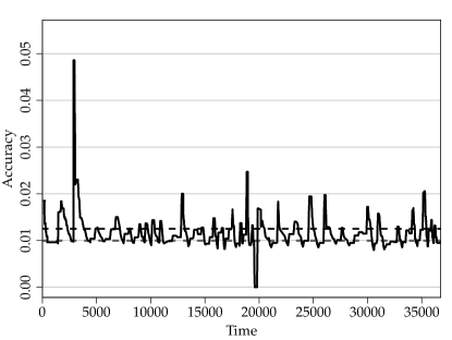
(a)

(b)

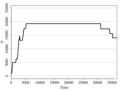
(c)

(d)

Figure 1: System results using $7$ day batches where (a) is the accuracy ($A$) of the predictions, (b) is the quality ($Q$) of the samples, (c) is the number of samples in the database ($N$) as new data are revealed and (d) is the Kaplan-Meier estimator the samples lifetime.

In order to determine the quality of the predicted ranks given by the system, we performed a separate run and consider the coverages of the prediction intervals. For this run the initial observations consisted of the 2005/06 to 2007/08 seasons results. We then introduced the match results for the 2008/09 to 2012/13 seasons in $7$ day batches. Over the $5$ seasons there were $178$ batches of intervals for each team. Before each batch of results was introduced, conservative $50$% and $95$% intervals were formed for the predicted end of season rank of each team. These confidence intervals are conservative due to the discreteness of ranks. The true mass contained in the conservative $50$% intervals was on average $76.1$%. Similarly, the true mass contained in the conservative $95$% intervals was on average $98.8$%. When compared with the true end of season ranks, $74.2$% of the true ranks lied in the conservative $50$% intervals and $99.3$% lied in the $95$% intervals.

4 Application to a Linear Gaussian Model

In §3 we are unable to check if the strengths of the teams and the other parameters (i.e. the states and parameters) are being estimated accurately as their true distributions are unknown. In this section we inspect the estimates given by the RMCMC system using simulated data. We use a linear Gaussian model such that the Kalman filter (Kalman, 1960) can be applied. This simulation will allow us to compare the RMCMC system and the Kalman filter estimates. This linear and Gaussian model was chosen to resemble the football model described in §3. For this model the Kalman filter gives the exact conditional distribution. Therefore, the Kalman filter will provide the benchmark estimates to compare against.

Consider the model defined as follows:

$$\begin{cases}\text{State}:\quad\quad\quad X_{t}=AX_{t-1}+\Phi_{t},&\Phi_{t}\stackrel{{\scriptstyle\text{iid}}}{{\sim}}\text{N}(0,\Sigma)\\ \text{Observation}:\quad Y_{t}=BX_{t}+\Psi_{t},&\Psi_{t}\stackrel{{\scriptstyle\text{iid}}}{{\sim}}\text{N}(0,\Xi)\end{cases},\quad\text{for }t=1,2,\dots$$ (2)

and prior distribution $X_{0}\sim\text{N}(\mu_{0},\Sigma_{0})$. For this particular simulation we chose $A=0.7(\mathbb{I}_{20}-\frac{1}{20}1_{20}1_{20}^{T})$, $\Sigma=0.05\mathbb{I}_{20}$ and $\Xi=0.02\mathbb{I}_{380}$. The matrix $B$ is constructed according to the football matches in the English Premier League in the $2005/06$ season. More precisely, each row of $B$ is consists of zeros apart from two entries at $i$ and $j$ corresponding to a football match between home team $i$ and away team $j$. A $2$ is put in the $i$th position and a $1$ at the $j$th. The rows are ordered chronologically from top to bottom. For the prior distribution, we set $\mu_{0}$ to be a vector of zeroes and $\Sigma_{0}=\mathbb{I}_{20}$. Denote the $i$th component of $X_{t}$ as $X_{i,t}$.

A single realisation of the states and observations were generated for $t=1,\dots,7$. Using these observations, the RMCMC system was run $100$ times to estimate means. This was compared with the estimates given by the Kalman filer. Each run of the RMCMC system was initialised using the observations from state $t=1,\dots,5$.

The sequence of targets is similar to that used in §3.1 with $\varpi_{k,t}=p(x_{1:t}|\widetilde{y}_{1:k,t},y_{1:(t-1)})$. For the transition function $f_{j}$ ($j\in D$) we use the observation equation in (2). Finally, we take $g_{n}$ to be the identity function, so that our estimate of interest in the posterior mean. The observations were revealed in batches of $10$, so that each state consisted of $38$ batches. Specifically, the vector $Y_{t}$ contains all $380$ observations where we denote the $j$th observation as $Y_{j,t}$. The $k$th observation batch of state $t$ is $\widetilde{Y}_{k,t}:=Y_{10k-9,t},\dots,Y_{10k,t}$. Therefore, after initialisation, the batches $\widetilde{Y}_{1,6},\dots,\widetilde{Y}_{38,6},\widetilde{Y}_{1,7},\dots\widetilde{Y}_{38,7}$ are revealed.

Within the control process we again use $\beta_{1}=0.01$, $\beta_{2}=0.0125$ and $\gamma_{1}=0.1$, $\gamma_{2}=0.75$. Also, we set $N_{\text{MIN}}=1,000$. For this simulation controlling the accuracy $A$ pertains to controlling the mean posterior of each component of every state as new data are observed. We use a Gibbs sampler (see e.g. Geman and Geman, 1984) as the conditional distributions for the states can be explicitly computed for this model. Each Gibbs sampler step consists of updating a single randomly chosen state as outlined in Algorithm 1. We used no subsampling and a burn-in period of $B_{0}=1,000$. The accuracy was calculated using the batch mean approach described in §2.7 with batch lengths $10$ and $25$. The RMCMC process wrote $500$ samples to the database at a time.

Algorithm 1 Gibbs Sampler: Single step

1:Given $X_{1},\dots,X_{n}$ and $Y_{1},\dots,Y_{n}$.

2:Generate $s\sim\text{Uniform}\{1,\dots,n\}$.

3:if $s=1$ then Draw $Z_{s}$ from the pdf $f(x_{1}|X_{2},\dots,X_{n},Y_{1},\dots,Y_{n})$.

4:if $s>1$ and $s<n$ then Draw $Z_{s}$ from the pdf $f(x_{s}|X_{1},\dots,X_{s-1},X_{s+1},\dots,X_{n},Y_{1},\dots,Y_{n})$.

5:if $s=n$ then Draw $Z_{s}$ from the pdf $f(x_{s}|X_{1},\dots,X_{n-1},Y_{1},\dots,Y_{n})$.

6:Let $X_{s}=Z_{s}$.

Figure 2 presents results comparing the Kalman filter estimates with the $100$ RMCMC estimates as the observations are revealed. The upper row of Fig 2 are violin plots (see e.g.  Hintze and Nelson, 1998) of the difference between the Kalman filter and the $100$ RMCMC system posterior mean of selected states and components. Violin plots are smoothed histograms either side of a box plot of the data.

The estimate may be bias due to the scaling and normalisation of the weights carried out by the update process (§2.4) (see for example Hesterberg (1995) for the bias in weighted importance sampling). This is apparent in posterior mean for $X_{18,6}$ (Fig. 2b), as in $81$ out of the $100$ runs the RMCMC process remained paused after $\widetilde{Y}_{37,6}$ was revealed. For these $81$ runs, the posterior mean was formed using weighted importance sampling. In contrast, we see nearly no bias in the posterior mean for $X_{5,6}$ after $\widetilde{Y}_{1,6}$ was revealed (Fig. 2a) where the RMCMC process was started in every run (the posterior mean given by the Gibbs sampler is unbiased). Table 6 shows the estimated bias of the $100$ RMCMC system posterior means with respect to estimate given by the Kalman filter. Table 7 shows the standard deviation of the $100$ RMCMC system posterior means. We see that the standard deviation (the accuracy $A$) is controlled below the imposed threshold of $\beta_{2}=0.0125$. The lower row of Fig 2 are Q-Q plots of the Kalman filter estimate and the weighted RMCMC samples posterior distribution at the $1\%,2\%,\dots,99\%$ quantile from $1$ of the $100$ runs. The Q-Q plots for other components of and RMCMC runs are similar to those presented. These Q-Q plots indicate that the two distributions are roughly similar.

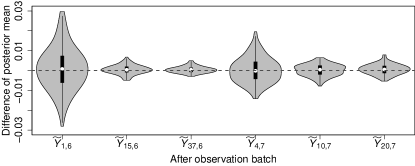
(a) Posterior Mean of $X_{5,6}$ and $X_{5,7}$.

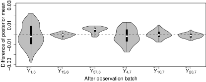
(b) Posterior Mean of $X_{18,6}$ and $X_{18,7}$.

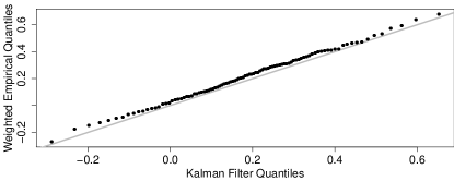
(c) Posterior mean of $X_{5,6}$ after $\widetilde{Y}_{1,6}$ revealed.

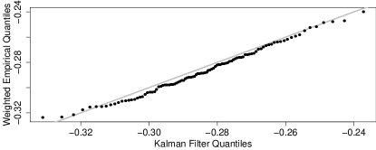
(d) Posterior mean of $X_{18,7}$ after $\widetilde{Y}_{20,7}$ revealed.

Figure 2: Simulation results: (a) and (b) are violin plots of the difference between the $100$ RMCMC and the Kalman filter posterior mean. (c) and (d) are Q-Q plots of the Kalman filter and RMCMC system posterior distribution from a single run (black).

Comparison of the two distributions is difficult as the RMCMC samples are not only weighted but are also dependent. Thus tests, such as the Kolmogorov-Smirnov test (e.g. see p. 35 Lehmann and D’Abrera, 1975), cannot be applied.

Table 6: Tables of estimated bias of the $100$ system posterior means with respect to Kalman filter posterior mean.

	Last batch revealed
	$\widetilde{Y}_{1,6}$	$\widetilde{Y}_{15,6}$	$\widetilde{Y}_{37,6}$
$X_{5,6}$	$0.0009$	$0.0004$	$0.0004$
$X_{18,6}$	$-0.0012$	$-0.0001$	$0.0049$

	Last batch revealed
	$\widetilde{Y}_{1,6}$	$\widetilde{Y}_{15,6}$	$\widetilde{Y}_{37,6}$
$X_{5,6}$	$0.0009$	$0.0004$	$0.0004$
$X_{18,6}$	$-0.0012$	$-0.0001$	$0.0049$

Table 7: Tables of the empirical standard deviation of posterior mean given by $100$ runs of the system.

	Last batch revealed
	$\widetilde{Y}_{1,6}$	$\widetilde{Y}_{15,6}$	$\widetilde{Y}_{37,6}$
$X_{5,6}$	$0.0109$	$0.0023$	$0.0016$
$X_{18,6}$	$0.0110$	$0.0019$	$0.0030$

	Last batch revealed
	$\widetilde{Y}_{3,7}$	$\widetilde{Y}_{10,7}$	$\widetilde{Y}_{20,7}$
$X_{5,7}$	$0.0065$	$0.0030$	$0.0026$
$X_{18,7}$	$0.0077$	$0.0037$	$0.0022$

5 Conclusion

We have presented a new method that produces estimates from a sequence of distributions that maintains the accuracy at a user-specified level. In §3 we demonstrated that the system is not resumed each time an observation is revealed thus the samples are reused. Therefore, we proceed with importance sampling whenever possible. Further we attempt to reduce the size of the sample database whenever possible (§2.5), thus limiting the computational effort of the update process and calculation of the estimates or predictions. In §4 we used a linear Gaussian model to show that the system produced comparable estimates to those given by the Kalman filter. Proving exactness of the estimates produced by the system, if possible, is a topic for future work.

For our system, we advocate using a standard MCMC method such as a Metropolis-Hastings algorithm before resorting to another more complicated method such as particle MCMC methods (Andrieu et al., 2010) or SMC² (Chopin et al., 2013). By starting with a standard MCMC approach, we avoid choosing the number of particles, choosing the transition densities and the resampling step that comes with using a particle filter, not to mention the higher computational cost.

Appendix A Further System Results

In this section we present further results from §4.5 in the main article. In Figure 3 we display the change of the accuracy of the predictions ($A$), the quality of the samples ($Q$) and the number of samples in the database ($N$) as new data are revealed. As expected, the larger the batch size the more frequently the accuracy of the predictions and the quality of the samples exceed the thresholds. Table 8, 9 and 10 present the predicted end of 2012/13 English Premier league ranks for the various batch sizes. The predictions are similar for all batch sizes. This is unsurprising since the predictions are based on the same data. Each probability (percentage) in Table 8, 9 and 10 are being controlled. More precisely, for each team and each rank the standard deviation of the reported probability (percentage) is being controlled below $\beta_{2}=0.0125$ (as set in the simulation in the main article §4.4).

The survival of the samples as new data are observed varies greatly depending on the batch size (Figure 4). From the Kaplan-Meier estimators in Fig 4a, 4b and 4c we observe that smaller batches increases the number of batches a sample survives. Hence, using smaller data batches results in samples being reused more.

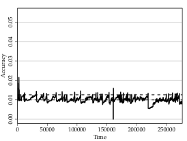
(a)

(b)

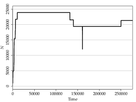
(c)

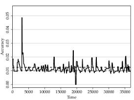
(d)

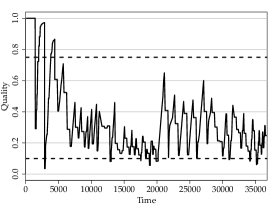
(e)

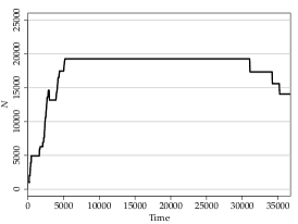
(f)

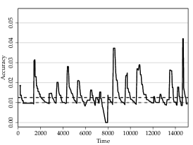
(g)

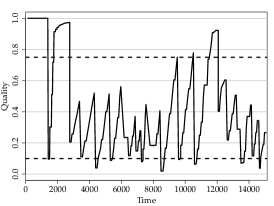
(h)

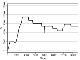
(i)

Figure 3: Panel of plots of the system variables as new data, of varying size, are observed. Columns, from left to right, are the accuracy of the predictions ($A$), the quality of the samples ($Q$) and the Number of samples in the database $N$. Rows, from top to bottom are for individual, weekly and monthly data sizes.

(a)

(b)

(c)

Figure 4: Kaplan-Meier estimators of the survival of the samples as new data are observed using (a) individual results, (b) 7 day batches and (c) 30 day batches.

Table 8: Predicted end of season 2012/13 ranks for the English Premier League using individual results reported in percent.

	Rank
Team	1	2	3	4	5	6	7	8	9	10	11	12	13	14	15	16	17	18	19	20
Arsenal	8	14	17	17	15	10	7	4	3	2	1	1	1	0	0	0	0	0	0	0
Aston Villa	0	0	1	1	3	3	5	6	7	7	8	8	8	7	8	7	6	6	5	4
Chelsea	9	15	19	17	13	9	6	4	2	2	1	1	1	0	0	0	0	0	0	0
Everton	1	2	6	8	11	11	12	10	9	7	6	5	4	3	2	1	2	1	1	0
Fulham	0	1	2	4	5	7	8	9	9	8	8	6	6	7	5	4	4	3	2	1
Liverpool	2	5	8	11	13	13	10	9	7	6	5	3	2	2	2	1	1	0	0	0
Man City	32	28	18	10	5	3	2	1	0	0	0	0	0	0	0	0	0	0	0	0
Man United	46	26	12	7	4	2	1	1	0	0	0	0	0	0	0	0	0	0	0	0
Newcastle	0	1	2	3	5	6	8	9	10	8	8	7	6	6	5	5	4	3	2	2
Norwich	0	0	0	1	1	2	3	4	4	6	6	8	8	8	8	9	9	8	9	7
QPR	0	0	0	0	0	1	2	2	3	5	5	6	6	7	8	9	9	11	13	12
Reading	0	0	0	0	1	1	2	2	4	4	5	5	7	7	7	9	9	10	12	14
Southampton	0	0	0	1	1	2	2	3	3	4	5	5	6	7	8	8	10	11	11	13
Stoke	0	0	1	1	2	3	4	6	7	7	7	8	8	7	8	7	7	7	7	5
Sunderland	0	0	1	2	4	5	6	8	8	8	8	8	7	7	6	6	5	4	4	3
Swansea	0	0	0	1	1	3	4	5	6	6	7	8	8	8	8	8	8	7	7	6
Tottenham	2	7	12	14	14	12	10	8	6	4	3	2	2	2	1	1	0	0	0	0
West Brom	0	0	0	1	2	3	4	5	6	8	7	8	8	8	7	8	7	7	5	5
West Ham	0	0	0	0	1	1	2	3	3	4	5	5	6	7	8	9	10	11	11	14
Wigan	0	0	0	0	1	1	2	2	3	4	5	6	7	8	9	9	10	10	11	13

Table 9: Predicted end of season 2012/13 ranks for the English Premier League using 7 day batches reported in percent.

	Rank
Team	1	2	3	4	5	6	7	8	9	10	11	12	13	14	15	16	17	18	19	20
Arsenal	8	14	17	19	13	9	6	4	3	2	2	1	1	0	0	0	0	0	0	0
Aston Villa	0	0	1	1	3	4	5	6	7	7	7	9	8	8	7	7	6	6	5	4
Chelsea	9	15	21	16	12	9	6	4	3	1	1	1	1	0	0	0	0	0	0	0
Everton	1	3	5	8	11	12	13	10	8	6	5	4	3	3	2	2	1	1	1	0
Fulham	0	1	2	3	5	6	8	9	9	9	9	7	7	5	5	4	4	3	3	2
Liverpool	2	4	7	11	15	13	10	9	7	6	4	3	3	2	2	1	1	1	0	0
Man City	29	27	18	10	6	4	2	1	0	0	0	0	0	0	0	0	0	0	0	0
Man United	47	26	14	7	3	1	1	0	0	0	0	0	0	0	0	0	0	0	0	0
Newcastle	0	1	2	3	5	7	9	9	8	9	8	7	7	6	6	4	3	3	2	1
Norwich	0	0	0	0	2	2	3	4	5	6	6	8	7	8	7	9	9	9	9	8
QPR	0	0	0	0	1	1	2	2	3	4	5	6	6	7	7	8	9	12	13	13
Reading	0	0	0	0	1	2	2	2	3	4	5	6	5	7	8	8	10	11	11	15
Southampton	0	0	0	0	0	1	2	2	3	5	5	5	6	7	8	9	9	10	12	13
Stoke	0	0	0	1	2	3	4	6	6	7	8	8	8	7	7	8	7	7	7	5
Sunderland	0	0	1	3	3	5	7	8	8	8	8	8	8	7	7	5	5	4	3	2
Swansea	0	0	0	1	1	2	3	4	6	6	7	7	8	8	8	8	9	8	7	6
Tottenham	4	8	11	14	14	13	10	8	6	4	3	2	1	1	1	1	0	0	0	0
West Brom	0	0	0	1	2	3	4	6	7	7	7	7	8	7	8	8	7	6	5	5
West Ham	0	0	0	0	1	1	2	3	3	5	4	5	7	7	9	9	9	11	11	14
Wigan	0	0	0	0	1	1	2	3	3	5	5	6	7	9	8	9	10	10	11	12

Table 10: Predicted end of season 2012/13 ranks for the English Premier League using 30 day batches reported in percent.

	Rank
Team	1	2	3	4	5	6	7	8	9	10	11	12	13	14	15	16	17	18	19	20
Arsenal	8	15	19	16	12	10	6	5	3	2	2	1	1	0	0	0	0	0	0	0
Aston Villa	0	0	1	1	2	4	6	6	7	7	7	8	8	7	6	7	6	6	5	3
Chelsea	10	16	20	16	12	9	6	4	2	2	2	1	0	1	0	0	0	0	0	0
Everton	1	2	5	8	11	10	10	10	9	8	5	5	3	3	2	1	2	1	1	0
Fulham	0	1	2	4	5	8	9	9	8	9	8	8	6	5	6	4	3	3	2	1
Liverpool	2	4	7	11	13	12	11	9	7	6	4	4	3	2	2	1	1	1	0	0
Man City	29	28	17	11	6	3	2	1	1	0	0	0	0	0	0	0	0	0	0	0
Man United	47	24	14	7	4	2	1	0	0	0	0	0	0	0	0	0	0	0	0	0
Newcastle	0	1	2	4	5	6	9	9	9	9	9	7	7	6	4	4	3	3	2	1
Norwich	0	0	0	0	1	2	2	4	5	6	7	7	7	8	8	8	8	8	9	9
QPR	0	0	0	0	0	1	2	2	3	4	4	4	7	7	8	9	10	11	12	14
Reading	0	0	0	0	1	2	2	2	3	5	4	5	7	7	8	8	9	10	12	14
Southampton	0	0	0	1	1	2	2	2	3	4	6	6	6	7	9	8	10	10	10	13
Stoke	0	0	0	1	2	2	4	6	5	7	7	8	7	8	8	8	8	7	6	5
Sunderland	0	0	1	2	4	6	6	7	8	8	7	8	8	7	6	6	4	5	4	2
Swansea	0	0	0	1	2	3	4	5	7	6	6	7	8	9	8	9	7	7	7	5
Tottenham	3	7	10	14	15	13	10	7	6	4	3	2	2	1	1	1	0	0	0	0
West Brom	0	0	1	1	2	4	4	5	7	8	8	7	8	7	7	7	6	7	6	5
West Ham	0	0	0	0	1	1	2	3	3	4	4	5	6	7	8	9	10	10	12	13
Wigan	0	0	0	0	1	1	2	2	3	4	5	6	6	7	7	9	11	11	12	13

References

- Andrieu et al. (2010) C. Andrieu, A. Doucet, and R. Holenstein. Particle Markov chain Monte Carlo methods. Journal of the Royal Statistical Society: Series B, 72(3):269–342, 2010.
- Brooks et al. (2011) S. Brooks, A. Gelman, G. Jones, and X. Meng. Handbook of Markov Chain Monte Carlo. CRC Press, 2011.
- Chopin (2002) N. Chopin. A sequential particle filter method for static models. Biometrika, 89(3):539–552, 2002.
- Chopin et al. (2013) N. Chopin, P. E. Jacob, and O. Papaspiliopoulos. SMC2: an efficient algorithm for sequential analysis of state space models. Journal of the Royal Statistical Society: Series B, 75(3):397–426, 2013.
- Del Moral et al. (2006) P. Del Moral, A. Doucet, and A. Jasra. Sequential Monte Carlo samplers. Journal of the Royal Statistical Society: Series B (Statistical Methodology), 68(3):411–436, 2006.
- Dixon and Coles (1997) M. J. Dixon and S. G. Coles. Modelling association football scores and inefficiencies in the football betting market. Journal of the Royal Statistical Society: Series C, 46(2):265–280, 1997.
- Doucet et al. (2001) A. Doucet, N. de Freitas, and N. Gordon, editors. Sequential Monte Carlo Methods in Practice. Springer, 2001.
- Flegal and Jones (2010) J. M. Flegal and G. L. Jones. Batch means and spectral variance estimators in Markov chain Monte Carlo. The Annals of Statistics, 38(2):1034–1070, 2010.
- Geman and Geman (1984) S. Geman and D. Geman. Stochastic relaxation, Gibbs distributions, and the Bayesian restoration of images. Pattern Analysis and Machine Intelligence, IEEE Transactions on, (6):721–741, 1984.
- Geyer (1992) C. J. Geyer. Practical Markov chain Monte Carlo. Statistical Science, 7(4):473–483, 1992.
- Glickman and Stern (1998) M. E. Glickman and H. S. Stern. A state-space model for National Football League scores. Journal of the American Statistical Association, 93(441):25–35, 1998.
- Gordon et al. (1993) N. Gordon, D. Salmond, and A. Smith. Novel approach to nonlinear/non-Gaussian Bayesian state estimation. Radar and Signal Processing, IEE Proceedings F, 140(2):107 –113, 1993.
- Gramacy et al. (2010) R. Gramacy, R. Samworth, and R. King. Importance tempering. Statistics and Computing, 20(1):1–7, 2010.
- Hastings (1970) W. K. Hastings. Monte Carlo sampling methods using Markov chains and their applications. Biometrika, 57(1):97–109, 1970.
- Hesterberg (1995) T. Hesterberg. Weighted average importance sampling and defensive mixture distributions. Technometrics, 37(2):185–194, 1995.
- Hintze and Nelson (1998) J. L. Hintze and R. D. Nelson. Violin plots: A box plot-density trace synergism. The American Statistician, 52(2):181–184, 1998.
- Jones (2004) G. L. Jones. On the Markov chain central limit theorem. Probability surveys, 1:299–320, 2004.
- Kalman (1960) R. E. Kalman. A new approach to linear filtering and prediction problems. Journal of basic Engineering, 82(1):35–45, 1960.
- Kaplan and Meier (1958) E. Kaplan and P. Meier. Nonparametric estimation from incomplete observations. Journal of the American Statistical Association,, 53:457–481, 1958.
- Kitagawa (2014) G. Kitagawa. Computational aspects of sequential Monte Carlo filter and smoother. Annals of the Institute of Statistical Mathematics, pages 1–29, 2014.
- Lahiri (2003) S. Lahiri. Resampling Methods for Dependent Data. Springer, 2003.
- Lehmann and D’Abrera (1975) E. L. Lehmann and H. D’Abrera. Nonparametrics: Statistical Methods Based on Ranks. Holden-Day, 1975.
- Liu (2008) J. S. Liu. Monte Carlo Strategies in Scientific Computing. Springer, 2008.
- Metropolis et al. (1953) N. Metropolis, A. W. Rosenbluth, M. N. Rosenbluth, A. H. Teller, and E. Teller. Equation of state calculations by fast computing machines. The Journal of Chemical Physics, 21(6):1087–1092, 1953.