Memory and long-range correlations in chess games

Abstract

In this paper we report the existence of long-range memory in the opening moves of a chronologically ordered set of chess games using an extensive chess database. We used two mapping rules to build discrete time series and analyzed them using two methods for detecting long-range correlations; rescaled range analysis and detrended fluctuation analysis. We found that long-range memory is related to the level of the players. When the database is filtered according to player levels we found differences in the persistence of the different subsets. For high level players, correlations are stronger at long time scales; whereas in intermediate and low level players they reach the maximum value at shorter time scales. This can be interpreted as a signature of the different strategies used by players with different levels of expertise. These results are robust against the assignation rules and the method employed in the analysis of the time series.

1 Introduction

Some games are complex systems which provide information about social and biological processes [2, 3, 4, 5, 6, 7, 8, 9, 10, 11, 12, 13]. They are currently being studied because of the existence of very well documented registers of games which are useful for statistical analysis. In particular, recent works have tried to understand the statistics of wins and losses in baseball teams [7], the final standing in basketball leagues [8], the distribution of career longevity in baseball [9], the football goal distribution [10], and face to face game rank distributions [11]. The time evolution of the table during a season, for instance, can be interpreted as a random walk [12], and long-range correlations have been found in the score evolution of the game of cricket [13]. Among them, the game of chess has a main place in occidental culture because its intrinsic complexity is viewed as a symbol of intellectual prowess. Since the skill level of chess players can be correctly identified [14] chess has contributed to the scientific understanding of expertise [6]. In addition, nowadays, there is a big world-wide community of chess players which makes the game a benchmark for studying, for instance, decision making processes [5] and population level learning [4].

Exploring a chess database Blasius and Tönjes [3] observed that the pooled distribution of all opening weights follows a Zipf law with universal exponent. This is a remarkable result [15, 16] since the Zipf law is followed in a range that comprises six orders of magnitude. In their work, the authors explain the results using a multiplicative process with a branching ratio distribution which resembles the real branching distribution measured in the database. Beyond the very good agreement between their empirical observations and the proposed model to explain Zipf’s law, they do not provide an explanation of the evolution of the pool of games; disregarding for instance, the question of possible memory effects between different games. The development of a given chess game should depend on the expertise of the players because the first moves (game opening) are usually known in advance by high level players as a result of their theoretical background. Other aspects can influence the development of a chess game according to the level of expertise. It has been established that skillful players develop outstanding rapid object recognition abilities that differentiate them from the non-expert players [17, 18]. In particular, Gobet and Simon [18] suggested that chess players, like experts in other fields, use long-term memory retrieval structures or templates in addition to chunks [19, 20] in short-term memory in order to store information rapidly. Then, it can be expected that the differences in the level of expertise of chess players are reflected in the historical development of chess databases introducing correlations between games through memory effects.

Currently there is a big corpus of digitized texts which allows the study of cultural trends tracing memory effects [21], opening a new branch in science known as culturomics [22]. In particular, long-range correlations have been observed in literary corpora [23, 24] where Zipf’s law was also studied using extensive databases [25]. Testing signatures of memory effects is important because it has been shown that systems which exhibit Zipf’s law need a certain degree of coherence [26] for its emergence. Therefore, the detection of long-range memory effects can be useful to shed light on the general mechanism behind the Zipf law.

In this work we explored the existence of long-range correlations in game sequences. To that end, time-series are constructed using a chronological ordered chess database similar to the one used by Blasius and Tönjes. In order to support the reliability of our results, we used two mapping rules to build the discrete time series. We also used different techniques to detect long-range correlations,namely the rescaled range analysis and the detrended fluctuation analysis [27].

2 Long-range correlation analysis

Rescaled range analysis ($R/S$) and detrended fluctuation analysis (DFA) are two useful tools for detecting long-range correlations in discrete time series. The $R/S$ analysis was introduced by Hurst when studying the regularization problem of the Nile River [27], whereas DFA was introduced by Peng et al. [28] for detecting long-range (auto-) correlations in time series with non-stationarities. Both methods use the accumulated time series which can be thought as the displacement of a one dimensional random walker whose steps are dictated by the values of the temporal series.

As a general procedure, the discrete time series $X(t)$ is first centered and normalized,

$$\tilde{X}(t)=\frac{X(t)-\langle X(t)\rangle}{\hat{\sigma}}$$ (1)

where $\hat{\sigma}=\sqrt{\langle X(t)^{2}\rangle-(\langle X(t)\rangle})^{2}$ and $\langle...\rangle$ means arithmetic averages over the complete series. Normalization is useful in order to compare different assignation rules [23]. Then the accumulated series $Y(t)$ is constructed,

$$Y(t)=\sum_{u=1}^{t}\tilde{X}(u).$$ (2)

Once the series $Y(t)$ is obtained, we applied the rescaled range analysis [23, 27] and the detrended fluctuation analysis [29, 30, 31]. In the $R/S$ method the time series $\tilde{X}(t)$ is divided into non-overlapping intervals of size $n$. The range of each interval is computed,

$$R(n)=max[Y(1),Y(2),...,Y(n)]-min[Y(1),Y(2),...,Y(n)],$$ (3)

and the corresponding standard deviation,

$$S(n)=\sqrt{\frac{1}{n}\sum_{i=1}^{n}{(X_{i}-m)}^{2}},$$ (4)

where $m$ is the average of $X(t)$ in the interval of size $n$. Then the average of the rescaled range $E[R(n)/S(n)]$ over all the intervals of size $n$ is calculated. The Hurst exponent $H$ is obtained varying the size of the intervals and fitting the data to the expression $Cn^{H}$ where $H$ is the Hurst exponent.

In the DFA method, the $Y(t)$ series is also segmented into intervals of size $n$. At each segment the cumulated series is fitted to a polynomial $y_{n}(t)$ and the fluctuation $F(n)$ is obtained:

$$F(n)=\sqrt{\frac{1}{N}\sum_{i=1}^{N}{[y(i)-y_{n}(i)]}^{2}},$$ (5)

where $N$ is the total number of data points. A log-log plot of F(n) is expected to be linear and if the slope is less than unity it corresponds to the Hurst exponent. When $H=0.5$ the time series resembles a memoryless random walker, and for $H>0.5$ ($H<0.5$) a random walker with persistent (antipersistent) long-range correlations.

3 Results

In our work we use the ChessDB database which has $3.5\times 10^{6}$ registered games; however, all our analysis is based on a subset of $1.4\times 10^{6}$ obtained by filtering corrupted data. The total time spanned in the database is about $10$ years, from $1998$ to $2007$. The first step in our analysis consists in mapping the chronologically ordered chess games into a discrete time series. The database contains approximately $380$ games per day uniformly distributed over $\approx 3650$ days. The games played on the same day are not chronologically ordered, hence the minimum time resolution in the studied temporal series is a day. The mapping for building the time series is far from being unique, but as a general rule it should not introduce spurious correlations [23, 24]. We used two assignation rules. In the first one, given a subset of consecutive games we evaluate the similitude of the last of them with the rest. We call this rule the similitude assignation rule (SAR). We chose to compare the recent $t$–th game against the rest using the following mapping expression,

$$X(t)=\sum_{t^{\prime}=t-\tau}^{t-1}S_{d}(t,t^{\prime}),$$ (6)

where $S_{d}(t,t^{\prime})=k\in\{0,1,2,3,...,d\}$ if and only if the $t$–th and $t^{\prime}$–th games are identical up to move $k$ included. Here $\tau+1$ is the total number of games in the set, and $d$ is the maximum number of moves to be considered. In this work we considered full length games, i.e. $d$ is the length of the shortest game to be compared. In our database the mean value of a game length is $\approx 60$ and the longest game corresponds to $400$ moves. According to Eq. (6) when $\tau=1$ then $X(t)=S_{d}(t,t-1)$, meaning that each point of the time series uses two consecutive games. For instance, if the sequence of moves of two games at $t$ and $t-1$ are –algebraic notation– $e4,e5;Nf3,Nc6;Bb5,a6;...$ and $e4,e5;Nf3,Nc6;d3,d6;...$, respectively, then $X(t)=4$ because these two games have four common moves. In the second rule, $X(t)$ is the popularity at depth $d$ of the t-th game, where the popularity at depth $d$ of the t-th game is equal to the number of games in the database that have the same moves up to depth $d$. We call this rule the popularity assignation rule (PAR) and is similar to the one introduced by Montemurro and Pury [23] for the study of a literary corpus. The popularity of a given game is computed using its firsts $d$ movements. Games that evolve in the same way up to a depth $d$ determine a subset of games with the same popularity. The popularity of a given game is equal to the number of elements of the subset to which it belongs. Notice that this assignation rule is based on a global characterization of the database; however, it does not introduce spurious correlations as we will see.

The mapping rules we have chosen are roughly equivalent since games with a popular sequence of movess are likely to match with other games. Popular games are related to opening lines which develop to different depths. From the chess opening system classification it is known that the game lines branch at different depths depending on the opening system, for instance, Caro-Kann opening has a long sequence of moves before branching. However, in a global characerization [3] the tree of chess moves has been proved to be self-similar to a certain degree, which means that the topology of the tree is nearly independent of the depth, supporting the equivalence of both mapping rules.

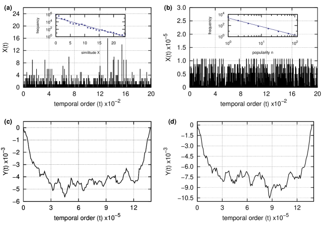
Figure 1: The top panels show fragments of the temporal series $X(t)$ (2000 points) obtained using the assignation by similitude (a) and popularity (b). The bottom panels show the complete integrated series, $Y(t)$, similitude (c) and popularity (d). Insets: distribution of similarities (a) and popularities (b). The straight lines correspond to fits using: $f(x)=Ae^{\alpha x}$ and $g(x)=Bx^{\beta}$, insets (a) and (b) respectively, where $\alpha=-0.49$ and $\beta=-1.53$.

The upper panels of Fig. 1 show fragments of the time series obtained using the two assignation rules described above. On the right, we show the PAR using a game depth $d=4$ and on the left the SAR using Eq.6 with $\tau=1$. These parameters are appropriated for comparing the two assignation rules. As we will see the mean value of the SAR series (with $\tau=1$) is small, meaning that the SAR is testing the first moves, therefore $d=4$ for the PAR is convenient. On the other hand, we have checked that the Hurst exponent is nearly independent of $d$ up to $d=20$. For $d>20$ correlations are affected maybe because the exponent of the power law which controls the distribution of popularities is much greater than 2, therefore fluctuations in the popularities become relevant [3]. In the SAR series the Hurst exponent is nearly independent of $\tau$ for $\tau\leq 500$. Beyond that value $H$ drops, and the SAR series do not show long-range correlations. Note that in the SAR case, increasing $\tau$ implies a sort of time averaging. The points of the series obtained by the PAR are distributed according to a scale free distribution as expected. In the corresponding inset we show this distribution, the exponent obtained by fitting is in agreement with that obtained by Blasius and Tönjes [3] (see caption). SAR series have small values since most of the matches between games are restricted to the first moves, in fact the distribution of coincidences is exponential and has a rapid decay (see inset and caption). This means that most of the consecutive games are similar in the very first moves, and a few of them have coincidences beyond the $10^{th}$ moves. In the bottom panels we show the complete accumulated series for both cases, SAR on the left and PAR on the right. Persistence can be appreciated from the monotonic behavior of the curve over long times.

In Fig. 2, we show data corresponding to the $R/S$ analysis (upper panel) and DFA (medium and lower panels). The left side panels show the analysis of the SAR series and the right one, that corresponding to the PAR series. In all cases a log-log plot of the points can be well fitted by a straight line as can be appreciated. The Hurst exponent obtained from both analyses $R/S$ and DFA are similar; however, the exponent tends to be larger in the PAR series, $H\simeq 0.75$ as compared to the SAR series $\simeq 0.67$. According to these values both series exhibit long-range correlations. Since SAR is a local assignation rule and PAR is based on a global charactarization of the database, SAR series should be noisier than PAR series. According to this the Hurst exponent of SAR is expected to be less than that of the PAR series. The fact that both methods give nearly the same value for the Hurst exponent indicates that non-stationarities are negligible in the time series. When the SAR and PAR time series are randomly shuffled (lower panels), the Hurst exponent in both analyses becomes close to $0.5$, which corresponds to series without long-range correlations. This means that the assignation rules we used do not introduce artificial correlations.

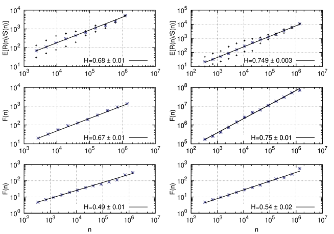
Figure 2: $R/S$ analysis (top panel) and DFA analysis (medium and lower panels) for the similitude (left) and popularity (right) assignation rules. The straight dashed lines are linear fits of the data. The $R/S$ error points (black crosses) correspond to the maximum and minimum point of the averaged data.

In order to compare the correlations obtained from different subsets of the total time series we will first study the dependence of the Hurst exponent on the length of the series. In the upper panel of Fig. 3 we plotted the Hurst exponent as function of the length $N$ of the PAR (full line) and SAR (dashed line) series. In all this analysis we used the DFA method and we averaged over all possible sets of consecutive games of length $N$. A certain correlation can be appreciated between the Hurst exponent of the two series assignations. The exponent $H$ of the PAR assignation is always greater than that of the SAR assignation, as in Fig.2. In both cases $H$ grows as the length of the series increases reaching a maximum value at nearly $2\times 10^{5}$ and then nearly stabilizes to $H\simeq 0.75$ in the PAR series and $H\simeq 0.65$ in the SAR series. In the case of the shuffled series (medium panel) we do not observe size effects and $H$ fluctuates around $0.5$ as expected. It is worth noting that in this analysis, a change in the size of the time series is equivalent to a change in the total time spanned. Finally, in the lower panel of Fig.3 we show the effects of reducing the series by pruning them. The error bars are obtained from the fitting errors. In this case we constructed reduced series by removing points from complete series but keeping nearly constant the total time span. More specifically, to construct the set of reduced series we pick up one point from the complete series every $s$ points, where $s=2,4,8,...$. The result after pruning is similar to that observed in the upper panel. In both cases, the exponent grows as the size of the series increases. However, in the pruned series $H$ seems not to be stabilized even in the larger series.

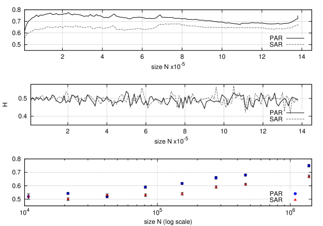
Figure 3: Upper panel: Hurst exponent obtained by the DFA method as function of the length of the time series using the two assignation rules, PAR and SAR series, full and dashed lines, respectively. Meddle panel: Hurst exponent obtained from the shuffled series. Lower panel: $H$ versus size in the pruned series.

Since the level of the players can be ranked according to their ELOs, a rating system introduced by the physicist Arpad Elo [14], we repeated the analysis filtering the database according to different ELO intervals. We used the following ELO’s ranges [6]: $[1,2199]$, $[2200,2399]$ and above $2400$. These intervals nearly correspond to: non-experts and master candidates, masters, and grand masters, respectively. In particular, this partition also ensures each interval contains nearly the same number of games. In Fig. 4, we show the Hurst exponent as function of the length of the time series associated to the ELO’s interval defined above. In the upper panel, we show the distribution of ELO’s rank of our database. As expected it is well described by a Gaussian function $\exp(\frac{-(x-x_{0})^{2}}{2a^{2}})$ (continuous line), with the fitted values, $x_{0}=2303$ and $a=203$. On the left we show the SAR series; and on the right, the PAR series. As in Fig. 3, the behavior of the two assignation rules is similar and the exponents of PAR series are slightly greater than in the SAR series. At short times the Hurst exponent in the three ELO intervals is close to 0.5, i.e. at this time scale games are uncorrelated and no persistence can be detected. At intermediate times, the lower ELO intervals show stronger correlations; and at the longest times, the order reverses and the games of high level players are the most correlated.

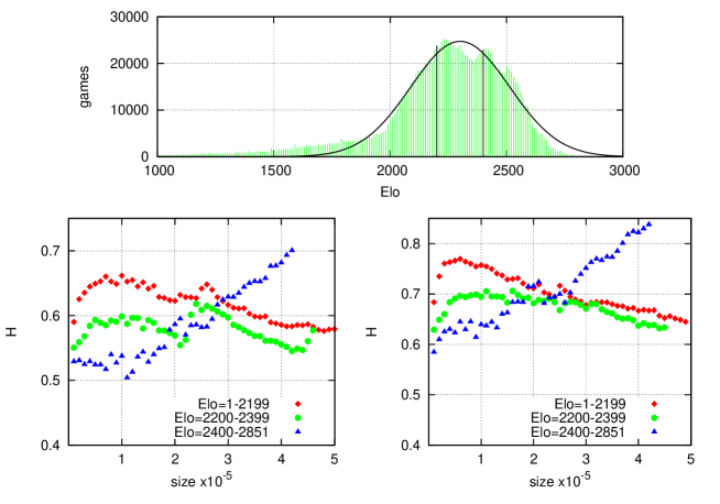
Figure 4: Hurst exponents obtained by the DFA method computed in different ELO intervals as function of the length of the series. SAR left lower panel and PAR rule right lower panel. Upper panel: ELO distribution of the whole database, the vertical lines indicates the ELO’s intervals. The continuous line correspond to a fit using a Gaussian function, $f(x)=\exp(\frac{-(x-x_{0})^{2}}{2a^{2}})$, with $x_{0}=2303$ and $a=203$.

When a pruning is implemented in series filtered according to ELO ranks, the Hurst exponent decreases as the length of the series decreases, as in the complete database (see Fig.5). The error bars are obtained from the fitting errors. At variance with the results of Fig.4 the series of higher ELOs are always more correlated, suggesting a different origin of this behavior.

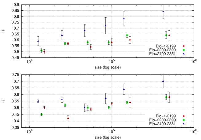
Figure 5: Size effects in the Hurst exponent for pruned series in different ELO ranges. Upper panel PAR series and lower panel SAR series.

4 Summary and Discussion

The Hurst exponents obtained through $R/S$ and DFA analysis are similar indicating that the time series analyzed are stationary for both assignation rules, SAR and PAR. For the case of PAR and the $R/S$ analysis our results are similar to that reported in literary corpora [23]. The value $H\simeq 0.5$ that emerges from the shuffled series implies that the assignation rules we used to build the series do not introduce spurious correlations. The analysis of the series as a function of the time spanned shows that there is a threshold in the length of the time series from which long-range correlations appear. This threshold depends on the assignation rule and on the level of the players. When the database is filtered by ELO ranks, our results indicate that long-range correlations observed at large time scales are related to the presence of high level players. The games corresponding to intermediate and low level players show correlations at shorter times when compared to high level players. A reduction of the database by pruning indicates that in short series correlations disappear. At variance with the analysis based on the length of the time spanned, the reduction in correlations by pruning has a similar behavior irrespective of the ELO ranks analyzed. Therefore, the reduction of correlations in this case should have a different origin.

Size effects in the detection of long-range correlations have been analyzed in the work of Coronado et al. [32] using time series generated by the Makse algorithm [33]. They observed that when DFA is used, size effects are negligible even in series containing as few as $10^{3}$ points. Since we use DFA and in our series size effects were observed in series having more than $10^{3}$ elements, our results must be reflecting intrinsic properties of the system. However, in our case we have portions of the time series which are randomly shuffled due to the minimum time resolution of our database, and this is affecting the detection of persistence in the time series. In long-memory analysis of persistence if missing data are replaced using random data drawn from the empirical distribution of the time series, the Hurst exponent tends to decrease [34]. Notice that pruning does not affect the total time spanned in the series. When pruning, the parameter $s$ can go up to $s\approx 380$ and still have on average one game per day in the pruned series with a time series of length $\approx 3,650$. According to this, the pruned time series we used should be representative samples of the temporal evolution of the games. However, as was pointed out, in pruned series correlations decrease. In our case, a possible explanation is that pruning affects the representativity of samples because persistence is a collective effect. The samples in order to be representative have to include at each time the behavior of a representative pool of different players. When series are pruned, the number of samples taken at the minimum resolution time (one day) are reduced hence the behavior of the pool of players is not correctly probed.

For intermediate and low level players persistence reaches its maximum in two or three years and then nearly stabilizes. This behavior is independent of the origin of time used for the analysis. In fact, the points shown in Fig. 4 result from the averaging of equivalent non-overlapping time intervals. For the most specialized players a signature of persistence appears after one or two years. According to our results, it seems that very high level players use different strategies as compared to low level players. It seems they vary the lines of play more often at short times scales, maybe because outstanding players know many opening lines in depth and are less influenced by the opponents. In particular, in high level players the correlations at large time scale are the strongest.

This work was partially supported by grants from CONICET, SeCyT–Universidad Nacional de Córdoba (Argentina), and the Academy of Finland, project no 260427. The authors thank Pedro Pury for useful discussion.

References

- [1]
- [2] F. Prost, On the impact of information technologies on society: an historical perspective through the game of chess, in: A. Voronkov (Ed.), Turing-100, Vol. 10 of EPiC Series, EasyChair, 2012, pp. 268–277.
- [3] B. Blasius, R. Tönjes, Zipf’s Law in the Popularity Distribution of Chess Openings, Phys. Rev. Lett. 103 (2009) 218701.
- [4] H. V. Ribeiro, R. S. Mendes, E. K. Lenzi, M. del Castillo-Mussot, L. A. N. Amaral, Move-by-move dynamics of the advantage in chess matches reveals population-level learning of the game, PLoS ONE 8 (1) (2013) e54165.
- [5] M. Sigman, P. Etchemendy, D. F. Slezak, G. A. Cecchi, Response time distributions in rapid chess: A large-scale decision making experiment, Frontiers in Neuroscience 4 (2010) 1.
- [6] P. Chassy, F. Gobet, Measuring chess experts’ single-use sequence knowledge: An archival study of departure from ’Theoretical’ openings, PLoS ONE 6 (11), PMID: 22110590 PMCID: PMC3217924.
- [7] C. Sire, S. Redner, Understanding baseball team standings and streaks, The European Physical Journal B 67 (3) (2009) 473–481.
- [8] Y. de Saá Guerra, J. M. González, S. S. Montesdeoca, D. R. Ruiz, A. García-Rodríguez, J. García-Manso, A model for competitiveness level analysis in sports competitions: Application to basketball, Physica A: Statistical Mechanics and its Applications 391 (10) (2012) 2997 – 3004.
- [9] A. M. Petersen, W.-S. Jung, H. E. Stanley, On the distribution of career longevity and the evolution of home-run prowess in professional baseball, EPL (Europhysics Letters) 83 (5) (2008) 50010.
- [10] E. Bittner, A. Nu baumer, W. Janke, M. Weigel, Football fever: goal distributions and non-gaussian statistics, The European Physical Journal B 67 (3) (2009) 459–471.
- [11] E. Ben-Naim, S. Redner, F. Vazquez, Scaling in tournaments, EPL (Europhysics Letters) 77 (3) (2007) 30005.
- [12] A. Heuer, O. Rubner, Fitness, chance, and myths: an objective view on soccer results, The European Physical Journal B 67 (3) (2009) 445–458.
- [13] H. V. Ribeiro, S. Mukherjee, X. H. T. Zeng, Anomalous diffusion and long-range correlations in the score evolution of the game of cricket, Phys. Rev. E 86 (2012) 022102.
- [14] M. E. Glickman, Chess rating systems, American Chess Journal 3 (1995) 59–102.
- [15] S. Maslov, Power laws in chess, Physics 2 (2009) 97.
- [16] Statistical physics: Chess obeys the law, Nature 462 (7273) (2009) 546–546.
- [17] F. Gobet, H. Simon, Recall of random and distorted chess positions: Implications for the theory of expertise, Memory & Cognition 24 (4) (1996) 493–503.
- [18] F. Gobet, H. A. Simon, Templates in chess memory: A mechanism for recalling several boards, Cognitive Psychology 31 (1) (1996) 1 – 40.
- [19] G. A. Miller, The magical number seven, plus or minus two: some limits on our capacity for processing information, Psychological Review 63 (2) (1956) 81–97.
- [20] W. G. Chase, H. A. Simon, Perception in chess, Cognitive Psychology 4 (1) (1973) 55 – 81.
- [21] C. Diuk, D. Fernandez Slezak, I. Raskovsky, M. Sigman, G. A. Cecchi, A quantitative philology of introspection, Frontiers in Integrative Neuroscience 6 (80).
- [22] J.-B. Michel, Y. K. Shen, A. P. Aiden, A. Veres, M. K. Gray, T. G. B. Team, J. P. Pickett, D. Hoiberg, D. Clancy, P. Norvig, J. Orwant, S. Pinker, M. A. Nowak, E. L. Aiden, Quantitative analysis of culture using millions of digitized books, Science 331 (6014) (2011) 176–182.
- [23] M. A. Montemurro, P. A. Pury, Long-range fractal correlations in literary corpora, Fractals 10 (04) (2002) 451–461.
- [24] E. G. Altmann, G. Cristadoro, On the origin of long-range correlations in texts, Proceedings of the National Academy of Sciences 109 (29) (2012) 11582–11587.
- [25] A. M. Petersen, J. N. Tenenbaum, S. Havlin, H. E. Stanley, M. Perc, Languages cool as they expand: Allometric scaling and the decreasing need for new words, Scientific Reports 2 (2012) 1.
- [26] M. Cristelli, M. Batty, L. Pietronero, There is more than a power law in zipf, Sci. Rep. 6 (80) (2012) 1–7.
- [27] J. Beran, Statistics for Long-Memory Processes, 1st Edition, Chapman-Hall, 1994.
- [28] C.-K. Peng, S. V. Buldyrev, S. Havlin, M. Simons, H. E. Stanley, A. L. Goldberger, Mosaic organization of dna nucleotides, Phys. Rev. E 49 (1994) 1685–1689.
- [29] C.-K. Peng, S. V. Buldyrev, A. L. Goldberger, S. Havlin, F. Sciortino, M. Simons, H. E. Stanley, Long-range correlations in nucleotide sequences, Nature 356 (6365) (1992) 168–170.
- [30] J. W. Kantelhardt, E. Koscielny-Bunde, H. H. Rego, S. Havlin, A. Bunde, Detecting long-range correlations with detrended fluctuation analysis, Physica A: Statistical Mechanics and its Applications 295 (3) (2001) 441–454.
- [31] R. M. Bryce, K. B. Sprague, Revisiting detrended fluctuation analysis, Scientific Reports 2 (315) (2012) 1–6.
- [32] A. Coronado, P. Carpena, Size effects on correlation measures, Journal of Biological Physics 31 (1) (2005) 121–133.
- [33] H. A. Makse, S. Havlin, M. Schwartz, H. E. Stanley, Method for generating long-range correlations for large systems, Phys. Rev. E 53 (1996) 5445–5449.
- [34] P. S. Wilson, C. A. Tomsett, R. Toumi, Long-memory analysis of time series with missing values, Phys. Rev. E 68 (2003) 017103.