Quantum dissipative effects in graphene-like mirrors

Abstract

We study quantum dissipative effects due to the accelerated motion of a single, imperfect, zero-width mirror. It is assumed that the microscopic degrees of freedom on the mirror are confined to it, like in plasma or graphene sheets. Therefore, the mirror is described by a vacuum polarization tensor $\Pi_{\alpha\beta}$ concentrated on a time-dependent surface. Under certain assumptions about the microscopic model for the mirror, we obtain a rather general expression for the Euclidean effective action, a functional of the time-dependent mirror’s position, in terms of two invariants that characterize the tensor $\Pi_{\alpha\beta}$. The final result can be written in terms of the TE and TM reflection coefficients of the mirror, with qualitatively different contributions coming from them. We apply that general expression to derive the imaginary part of the ‘in-out’ effective action, which measures dissipative effects induced by the mirror’s motion, in different models, in particular for an accelerated graphene sheet.

I Introduction

One of the most remarkable manifestations of the quantum nature of the electromagnetic (EM) field is the so called ‘motion induced radiation’ or ‘Dynamical Casimir Effect’ (DCE), whereby the accelerated motion of a mirror can make the EM field vacuum to evolve to an excited state, namely, one containing a non-vanishing number of photons moore .

Predictions about potentially observable DCE effects have been obtained for a variety of geometries and systems, and by means of quite different theoretical tools reviews . In this paper we concentrate on the calculation of DCE effects for the case of ‘imperfect mirrors’, by which we mean those that do not necessarily impose perfect conductor boundary conditions.

To conduct this study, we shall follow our previous work for scalar and spinorial vacuum fields prd07 ; prd11 in which we used the particularly convenient functional approach proposed in Ref.GK . This approach is based on the introduction of auxiliary fields inside the functional integral for the vacuum field, whose role is to impose the proper boundary conditions for the scalar field on each mirror. We shall here use an adapted version of the method, designed to deal with the case of imperfect mirrors, in the presence of the quantum EM field.

In a recent work maghrebi , the DCE for imperfect mirrors has been analyzed using a scattering approach, for the case of a quantum scalar field. Here, instead, we will consider the EM case, and for mirrors that can be described by means of their vacuum polarization tensors (VPT), which in turn are assumed to come from the integration of charged microscopic degrees of freedom constrained to them. Our results are therefore applicable, for instance, to plasma and graphene sheets.

Formally, we will compute the Euclidean effective action, and use analytic continuation to obtain the imaginary part of the real-time ‘in-out’ effective action. The latter is proportional to the probability of vacuum decay, an effect due to the mirror’s acceleration.

The paper is organized as follows: in Section II, we describe the kind of system that we shall consider, and define the corresponding effective action, within the framework of a perturbative expansion in powers of the departure of the mirror from its equilibrium position (a planar, static configuration). We obtain a general expression for the effective action at the second order in that expansion, in terms of two scalar functions which entirely define the response functions of the mirror. Moreover, up to this order, the result can be written as an integral that involves the transverse electric (TE) and transverse magnetic (TM) reflection coefficients of the mirror.

In Section III we evaluate the Euclidean effective action for different examples, discarding terms that do not contribute to the imaginary part of the vacuum energy (i.e., to the vacuum decay probability) when rotated back to Minkowski spacetime. The examples considered are distinguished by the different choices for the mirror’s VPT. We consider, in particular, the VPT corresponding to a graphene sheet described by massless fermions.

We present our conclusions in Section IV.

II The model and its Euclidean effective action

II.1 The model

We shall begin by defining here the characteristics of the system and its geometry, as well as the conventions and approximations adopted to describe it.

Euclidean spacetime coordinates $x_{0},x_{1},x_{2},x_{3}$, with the metric $(g_{\mu\nu})={\rm diag}(1,1,1,1)$ are used. The (vacuum) fluctuating field is assumed to be an Abelian gauge field $A_{\mu}$, with $\mu=0,1,2,3$, interacting with a zero-width mirror. This interaction is realized, in a linear response approximation, via the VPT due to a medium confined to a surface. An approximation will be implemented here, regarding this object: the surface curvatures shall be assumed to be sufficiently small as to allow for a description where the linear response function corresponding to a plane can be used locally. In other words, at each tangent plane, we shall use the VPT due to a plane mirror. The rationale behind this approximation, as well as the kind of effect that are neglected by its implementation are discussed below.

The most general kind of motion we shall deal with, amounts to a mirror whose shape and position can be defined by a single scalar function $\psi$, such that $x_{3}=\psi(x_{\parallel})$, where $x_{\parallel}\equiv(x_{0},x_{1},x_{2})$. Inside this general situation we shall focus on an interesting particular case, namely, a situation where the mirror’s surface is defined by an equation of the form $x_{3}=q(x_{0})$, i.e., a rigidly moving infinite plane. The reason for considering this case is that it will allow us to find explicit expressions for some interesting models. Nevertheless, expressions corresponding to more general functions will also be presented in the result for the effective action.

We would like to stress that, to make the calculations in Euclidean spacetime, is in no way mandatory; rather, it is a technique that, in some situations, may simplify the intermediate calculations without altering the underlying physics. For the particular problem of moving mirrors, the Euclidean formalism has already been used in Ref.GK . The connection with the “in-out” and “in-in” formalisms has been discussed in detail in our previous work prd07 . For more general discussions see Ref.vilkov .

The Euclidean action ${\mathcal{S}}$ is assumed to fall under the general structure:

$${\mathcal{S}}\;=\;{\mathcal{S}}(A,\psi)\,=\,{\mathcal{S}}_{0}(A)\,+\,{\mathcal{S}}_{I}(A,\psi)\;,$$ (1)

where $S_{0}$ denotes the free action for the electromagnetic field

$${\mathcal{S}}_{0}(A)\,=\,\frac{1}{4}\int F_{\mu\nu}F_{\mu\nu}\;,$$ (2)

where $\mu,\nu$ and, in general, indices from the middle of the Greek alphabet are assumed to run from $0$ to $3$. On the other hand, ${\mathcal{S}}_{I}(A,\psi)$ accounts for the coupling between $A$ and the microscopic degrees of freedom on the moving mirror. To construct it, we start by defining it in the case of a flat and static mirror at $x_{3}=\psi_{0}={\rm constant}$:

$${\mathcal{S}}_{I}(A,\psi_{0})\;=\;\frac{1}{2}\int_{x_{\parallel},y_{\parallel}}A_{\alpha}(x_{\parallel},\psi_{0})\Pi^{\alpha\beta}(x_{\parallel}-y_{\parallel})A_{\beta}(y_{\parallel},\psi_{0})\;,$$ (3)

where $\Pi^{\alpha\beta}(x_{\parallel}-y_{\parallel})$ denotes the VPT for the medium on the plane sheet, and $\alpha,\beta=0,1,2$. It depends, in this case, on the difference between its arguments, because of the (assumed) homogeneity of the medium. We are working in the usual linear response approximation, in which one retains only the quadratic terms in the gauge field.

Note that the component of the gauge field which is normal to the mirror’s plane ($A_{3}$) does not couple to the medium, something which is perfectly consistent with the assumption about the mirror to have zero width, since in this case the current associated to the microscopic degrees of freedom is confined to the plane.

We consider now the general form of the interaction term for a moving and deformed mirror described by $x_{3}=\psi(x_{\parallel})$. Formally, the integration of the microscopic degrees of freedom must be performed in a curved hypersurface, whose induced metric reads

$$g_{\alpha\beta}(x_{\parallel})\;=\;\delta_{\alpha\beta}+\partial_{\alpha}\psi(x_{\parallel})\,\partial_{\beta}\psi(x_{\parallel})\;.$$ (4)

Therefore, on general grounds we expect the interaction term to have the covariant expression

$${\mathcal{S}}_{I}(A,\psi) = \frac{1}{2}\,\int_{x_{\parallel},y_{\parallel}}\sqrt{g(x_{\parallel})}\sqrt{g(y_{\parallel})}\,A_{\alpha}(x_{\parallel},\psi(x_{\parallel}))$$ (5)

$$\times \,\Pi_{g}^{\alpha\beta}(x_{\parallel},y_{\parallel})A_{\beta}(y_{\parallel},\psi(y_{\parallel}))$$

where $g(x_{\parallel})=\det[g_{\alpha\beta}(x_{\parallel})]=1+\partial_{\alpha}\psi(x_{\parallel})\partial_{\alpha}\psi(x_{\parallel})$.

The components of the gauge fields which are parallel the mirror ($A_{\alpha}$) can be written in terms of the components in the laboratory frame ($A_{\mu}$) using three tangent vectors to the world-volume swept by the mirror during its time evolution:

$$e^{\mu}_{\alpha}(x_{\parallel})\,=\,\delta^{\mu}_{\alpha}\,+\,\delta^{\mu}_{3}\,\partial_{\alpha}\psi(x_{\parallel})\;$$ (6)

as follows

$$A_{\alpha}(x_{\parallel})=e^{\mu}_{\alpha}(x_{\parallel})A_{\mu}(x_{\parallel}).$$ (7)

Note that, unlike for a flat and static mirror, the interaction term contains the laboratory frame component $A_{3}$.

$\Pi^{\alpha\beta}_{g}(x_{\parallel},y_{\parallel})$ in Eq. (5) denotes the VPT for the medium on the curved mirror (the subindex $g$ emphasizes the dependence of the VPT with the induced metric). For an arbitrary $\psi$, this is a rather involved object, which can be computed, in principle, using techniques of quantum field theory in curved spacetimes. We shall assume that the induced metric is almost flat, i.e. $g_{\alpha\beta}\simeq\delta_{\alpha\beta}$. Physically, this means that at each time the mirror is gently curved, and that its motion involves non-relativistic velocities, so that $\partial_{\alpha}\psi(x_{\parallel})\,\partial_{\beta}\psi(x_{\parallel})\ll 1$.

We proceed as usual and expand the VPT around the flat metric

$$\Pi^{\alpha\beta}_{g}(x_{\parallel},y_{\parallel}) \simeq \Pi^{\alpha\beta}(x_{\parallel}-y_{\parallel})+\Delta\Pi^{\alpha\beta}_{g}(x_{\parallel},y_{\parallel})$$ (8)

$$= \Pi^{\alpha\beta}(x_{\parallel}-y_{\parallel})+O(\psi^{2})\,,$$

where the first term is the flat VPT and the first correction, linear in the metric, will be quadratic in $\psi$. One could compute $\Delta\Pi^{\alpha\beta}_{g}(x_{\parallel},y_{\parallel})$, using, for instance a covariant perturbation theory vilkov . However, as we will see, the flat VPT will be enough for our purposes.

Our next step is to introduce $\Gamma(\psi)$, the effective action for the mirror’s configuration:

$$e^{-\Gamma(\psi)}\,=\,\frac{{\mathcal{Z}}(\psi)}{{\mathcal{Z}}(0)}\;,$$ (9)

where

$${\mathcal{Z}}(\psi)\,=\,\int[{\mathcal{D}}A]\;e^{-{\mathcal{S}}(A,\psi)}\;,$$ (10)

and $[{\mathcal{D}}A]$ is the path integral measure including gauge fixing.

II.2 Auxiliary fields

Then we use an equivalent way of writing the $S_{I}$ term, by means of an auxiliary field $\xi^{\alpha}(x_{\parallel})$, a vector field in $2+1$ dimensions:

$$e^{-{\mathcal{S}}_{I}(A,\psi)} = {\cal N}\,\,\int{\mathcal{D}}\xi\,\delta(\nabla\cdot\xi)$$

$$\times e^{-\frac{1}{2}\int_{x_{\parallel},y_{\parallel}}\xi^{\alpha}(x_{\parallel})\Lambda_{\alpha\beta}(x_{\parallel},y_{\parallel})\xi^{\beta}(y_{\parallel})+i\int_{x}J_{\mu}(x)A_{\mu}(x)}$$

where we introduced $J^{\mu}(x)$, a current concentrated on the mirror’s world-volume:

$$J^{\mu}(x)\,=\,\sqrt{g(x_{\parallel})}\,e^{\mu}_{\alpha}(x_{\parallel})\,\delta(x_{3}-\psi(x_{\parallel}))\,\xi^{\alpha}(x_{\parallel})\;,$$ (12)

and $\Lambda_{\alpha\beta}(x_{\parallel},y_{\parallel})$ is the inverse (with respect to continuous and discrete indices) of $\Pi_{g}^{\alpha\beta}(x_{\parallel},y_{\parallel})$. The inverse is understood on the space of fields satisfying $\nabla_{\alpha}\xi^{\alpha}=0$, the covariant divergence of the auxiliary field. The reason for introducing the factor with a functional $\delta$-function of this divergence has to do with the transverse nature of the vacuum polarization tensor (Ward-Takahashi identities): the Gaussian representation used in Eq.(II.2) has to be constructed not with unconstrained vector fields but rather only with transverse ones. Indeed, $\Pi_{g}^{\alpha\beta}$ is invertible, and has $\Lambda_{\alpha\beta}$ as its inverse, on the subspace of transverse fields. Besides, the condition on the divergence of the auxiliary field implies the conservation of $J^{\mu}$, and hence the invariance of the action under gauge transformations $A_{\mu}\to A_{\mu}+\partial_{\mu}\omega$.

Using now Eq.(II.2) in Eq.(10), and integrating out $A$, we see that:

$${\mathcal{Z}}(\psi)\,=\,{\mathcal{Z}}_{0}\,{\cal N}\,\int{\mathcal{D}}\xi\,\delta(\nabla\cdot\xi)\,e^{-{\mathcal{S}}_{\rm eff}(\xi)}$$ (13)

where ${\mathcal{Z}}_{0}$ is the vacuum amplitude for the free electromagnetic field, and

$${\mathcal{S}}_{\rm eff}(\xi)\,=\,\frac{1}{2}\int_{x_{\parallel},y_{\parallel}}\xi^{\alpha}(x_{\parallel}){\mathcal{K}}_{\alpha\beta}(x_{\parallel},y_{\parallel})\xi^{\beta}(y_{\parallel})\;,$$ (14)

where

$${\mathcal{K}}_{\alpha\beta}(x_{\parallel},y_{\parallel}) = \sqrt{g(x_{\parallel})}\,e^{\mu}_{\alpha}(x_{\parallel})\,G_{\mu\nu}\big{(}x_{\parallel}-y_{\parallel},\psi(x_{\parallel})-\psi(y_{\parallel})\big{)}$$ (15)

$$\times e^{\nu}_{\beta}(y_{\parallel})\,\sqrt{g(y_{\parallel})}+\Lambda_{\alpha\beta}(x_{\parallel},y_{\parallel})\;,$$

with $G_{\mu\nu}(x-y)$ denoting the gauge field propagator. We have found it convenient to use the Feynman gauge, so that

$$G_{\mu\nu}(x-y)\;=\;\delta_{\mu\nu}\int\frac{d^{4}k}{(2\pi)^{4}}\,\frac{e^{ik\cdot(x-y)}}{k^{2}}\;.$$ (16)

Note that, since the auxiliary field is constrained to verify $\nabla\cdot\xi=0$, in Eq.(14) we may discard from ${\mathcal{K}}_{\alpha\beta}$ any contribution which vanishes when acting on the subspace of fields satisfying that condition.

II.3 Second order expansion

Let us now implement the second order perturbative expansion for the effective action $\Gamma(\psi)$ to the second order in $\psi$, the departure of the mirror from its average position. We first note that the formal result of integrating out the auxiliary field is:

$$\Gamma(\psi)\,=\,\frac{1}{2}\,\Big{[}{\rm Tr}\log{\mathcal{K}}\,-\,{\rm Tr}\log{\mathcal{K}}|_{\psi\equiv 0}\Big{]}\;.$$ (17)

Denoting by ${\mathcal{K}}^{(a)}$ the $a^{th}$-order term in an expansion in powers of $\psi$, we obtain the corresponding expansion of $\Gamma$. The $0^{th}$-order term vanishes, as well as the first-order term, while the second-order term $\Gamma^{(2)}$ becomes:

$$\Gamma^{(2)}(\psi)\,=\,\frac{1}{2}\,{\rm Tr}\Big{[}\big{(}{\mathcal{K}}^{(0)}\big{)}^{-1}{\mathcal{K}}^{(2)}\big{]}\;.$$ (18)

In this approximation, the effective action will be of the form

$$\Gamma^{(2)}(\psi)\;=\;-\frac{1}{2}\int_{x_{\parallel},x^{\prime}_{\parallel}}\,\psi(x_{\parallel})F(x_{\parallel},x^{\prime}_{\parallel})\psi(x^{\prime}_{\parallel})$$ (19)

for some two-point function $F$. As we are interested in dissipative effects, we may neglect any contribution to $\Gamma^{(2)}$ which is local in derivatives of $\psi$. This will simplify the calculations below.

The explicit form of the zeroth-order kernel, which is translation invariant, is

$${\mathcal{K}}^{(0)}_{\alpha\beta}(x_{\parallel},y_{\parallel})\,=\,\int\frac{d^{3}k_{\parallel}}{(2\pi)^{3}}\,e^{ik_{\parallel}\cdot(x_{\parallel}-y_{\parallel})}\,\widetilde{\mathcal{K}}^{(0)}_{\alpha\beta}(k_{\parallel})$$ (20)

where

$$\widetilde{\mathcal{K}}^{(0)}_{\alpha\beta}(k_{\parallel})\,=\,\frac{1}{2|k_{\parallel}|}{\mathcal{P}}^{\perp}_{\alpha\beta}(k_{\parallel})\,+\,\widetilde{\Lambda}^{(0)}_{\alpha\beta}(k_{\parallel})\;,$$ (21)

$\widetilde{\Lambda}^{(0)}_{\alpha\beta}$ is the Fourier transform of the inverse of the flat VPT and ${\mathcal{P}}^{\perp}_{\alpha\beta}\equiv\delta_{\alpha\beta}-\frac{k_{\alpha}k_{\beta}}{k_{\parallel}^{2}}$.

Regarding the second-order object ${\mathcal{K}}^{(2)}$, it receives many different contributions. However, as already stressed, we are here interested only in the calculation of dissipative terms. Thus, we may ignore any term producing a local contributions. In particular, as the deviation of the induced metric from the identity tensor is already quadratic in $\psi$, we can replace it by the identity tensor. For the same reason, we can omit the corrections to the flat VPT in Eq.(8), and replace $\Lambda_{\alpha\beta}$ by $\Lambda^{(0)}_{\alpha\beta}$ in Eq.(15). Note however, that there will be a non trivial contribution from the tangent vectors $e_{\alpha}^{\mu}$, that contain terms linear in $\psi$. Thus,

$${\mathcal{K}}^{(2)}_{\alpha\beta}(x_{\parallel},y_{\parallel}) = -\frac{1}{2}\psi(x_{\parallel})\psi(y_{\parallel})\,\int\frac{d^{3}k_{\parallel}}{(2\pi)^{3}}\,e^{ik_{\parallel}\cdot(x_{\parallel}-y_{\parallel})}\,|k_{\parallel}|\delta_{\alpha\beta}$$ (22)

$$+ \partial_{\alpha}\psi(x_{\parallel})\partial_{\beta}\psi(y_{\parallel})\,\int\frac{d^{3}k_{\parallel}}{(2\pi)^{3}}\,\frac{e^{ik_{\parallel}\cdot(x_{\parallel}-y_{\parallel})}}{2|k_{\parallel}|}\;.$$

We may obtain a more explicit formula for the second order contribution to $\Gamma$, by taking into account the structure of the VPT, which appears in $\widetilde{\mathcal{K}}^{(0)}$. Under the assumption of invariance under spatial rotations on $x_{3}$=constant planes, this tensor can be decomposed into orthogonal projectors. Indeed, since:

$$k_{\alpha}\widetilde{\Pi}^{\alpha\beta}\;=\;0\;,$$ (23)

the irreducible tensors (projectors) along which $\widetilde{\Pi}_{\alpha\beta}$ may be decomposed must satisfy the condition above and may be constructed using as building blocks the objects: $\delta_{\alpha\beta}$, $k_{\alpha}$, and $n_{\alpha}=(1,0,0)$. By performing simple combinations among them, we also introduce: $\breve{k}_{\alpha}\equiv k_{\alpha}-k_{0}n_{\alpha}$, and $\breve{\delta}_{\alpha\beta}\equiv\delta_{\alpha\beta}-n_{\alpha}n_{\beta}$.

Then we construct two independent tensors satisfying the transversality condition, ${\mathcal{P}}^{t}$ and ${\mathcal{P}}^{l}$, defined as follows:

$${\mathcal{P}}^{t}_{\alpha\beta}\,\equiv\,\breve{\delta}_{\alpha\beta}-\frac{\breve{k}_{\alpha}\breve{k}_{\beta}}{\breve{k}^{2}}$$ (24)

and

$${\mathcal{P}}^{l}_{\alpha\beta}\,\equiv\,{\mathcal{P}}^{\perp}_{\alpha\beta}\,-\,{\mathcal{P}}^{t}_{\alpha\beta}\;.$$ (25)

Defining also:

$${\mathcal{P}}^{\shortparallel}_{\alpha\beta}\,\equiv\,\frac{k_{\alpha}k_{\beta}}{k^{2}}\;.$$ (26)

we find the following algebraic properties:

$${\mathcal{P}}^{\perp}+{\mathcal{P}}^{\shortparallel}=I\;,\;\;{\mathcal{P}}^{t}+{\mathcal{P}}^{l}={\mathcal{P}}^{\perp}$$

$${\mathcal{P}}^{t}{\mathcal{P}}^{l}={\mathcal{P}}^{l}{\mathcal{P}}^{t}=0\;,\;\;{\mathcal{P}}^{\shortparallel}{\mathcal{P}}^{t}={\mathcal{P}}^{t}{\mathcal{P}}^{\shortparallel}=0\;,$$

$$\;\;{\mathcal{P}}^{\shortparallel}{\mathcal{P}}^{l}={\mathcal{P}}^{l}{\mathcal{P}}^{\shortparallel}=0\;,$$

$$\big{(}{\mathcal{P}}^{\perp}\big{)}^{2}={\mathcal{P}}^{\perp}\;,\big{(}{\mathcal{P}}^{\shortparallel}\big{)}^{2}={\mathcal{P}}^{\shortparallel}\;,\big{(}{\mathcal{P}}^{t}\big{)}^{2}={\mathcal{P}}^{t}\;,\big{(}{\mathcal{P}}^{l}\big{)}^{2}={\mathcal{P}}^{l}\;.$$ (27)

For a general medium, we shall have:

$$\widetilde{\Pi}_{\alpha\beta}(k)\,=\,g_{t}\big{(}k_{0},{\mathbf{k}}_{\parallel}\big{)}\,{\mathcal{P}}^{t}_{\alpha\beta}\,+\,g_{l}\big{(}k_{0},{\mathbf{k}}_{\parallel}\big{)}\,{\mathcal{P}}^{l}_{\alpha\beta}\;,$$ (28)

where $g_{t}$ and $g_{l}$ are model-dependent scalar functions.

In what follows, we particularize to the case of the rigid motion of a flat mirror along its normal direction, i.e. $\psi(x_{\parallel})=q(x_{0})$. In this case $\Gamma^{(2)}$ has the form:

$$\frac{1}{L^{2}}\Gamma^{(2)}\; = \;-\frac{1}{2}\int_{x_{0},x^{\prime}_{0}}\,q(x_{0})f(x_{0}-x^{\prime}_{0})q(x^{\prime}_{0})$$ (29)

$$= \frac{1}{2}\int dp_{0}{\tilde{f}}(p_{0})|\tilde{q}(p_{0})|^{2}\,,$$

where $L^{2}$ denotes the area of the $x_{1},x_{2}$ space. Using the projectors introduce above, after some algebra, we see that ${\tilde{f}}(p_{0})$, the Fourier transform of $f$, naturally decomposes as follows:

$${\tilde{f}}(p_{0})\,=\,{\tilde{f}}_{t}(p_{0})+{\tilde{f}}_{l}(p_{0})$$ (30)

where

$${\tilde{f}}_{t}(p_{0})\;=\;\int\frac{d^{3}k_{\parallel}}{(2\pi)^{3}}\;r_{t}(k_{\parallel})\,|k_{\parallel}|\,\sqrt{(k_{0}+p_{0})^{2}+{\mathbf{k}_{\parallel}}^{2}}\;,$$ (31)

and

$${\tilde{f}}_{l}(p_{0}) = \int\frac{d^{3}k_{\parallel}}{(2\pi)^{3}}\;r_{l}(k_{\parallel})\,\left[|k_{\parallel}|\,\sqrt{(k_{0}+p_{0})^{2}+{\mathbf{k}_{\parallel}}^{2}}\right.$$ (32)

$$- \left.\frac{{\mathbf{k}_{\parallel}}^{2}\,p_{0}^{2}}{|k_{\parallel}|\sqrt{(k_{0}+p_{0})^{2}+{\mathbf{k}_{\parallel}}^{2}}}\right]\;,$$

where

$$r_{t,l}(|k_{\parallel}|)\,=\,\frac{1}{1+\frac{2|k_{\parallel}|}{g_{t,l}(k_{\parallel})}}\;.$$ (33)

The decomposition in Eqs.(30)-(32), the main general result of this article, implies that the EM field problem is decomposed into two independent contributions, one due to $r_{t}$ and the other to $r_{l}$, which, as we will see below, are the Euclidean version of the TE and TM mirror’s reflection coefficients.

The dissipative effects can be obtained from the imaginary part of the real time “in-out” effective action $\Gamma^{(2)}_{\rm in-out}$, which is related to the probability $P$ of producing a photon pair out of the vacuum vpa through

$$P\simeq 2\,{\rm Im}[\Gamma^{(2)}_{\rm in-out}]\,.$$ (34)

The “in-out” effective action can be obtained from the Euclidean effective action performing a Wick rotation. From Eq.(29) we obtain

$$\frac{\Gamma^{(2)}_{\rm in-out}}{L^{2}}=\frac{1}{2}\int dp_{0}[{\tilde{f}}_{t}(ip_{0})+{\tilde{f}}_{l}(ip_{0})]|\tilde{q}(p_{0})|^{2}\,,$$ (35)

where $\tilde{q}(p_{0})$ denotes the Fourier transform of the physical trajectory in Minkowski spacetime.

It is noteworthy that the coefficients $r_{t,l}$ appearing in Eq.(33) and in the final formula for the effective action are just the static TE and TM reflection coefficients of the mirror. Indeed, in Ref. fialkovsky it has been shown that for a thin mirror characterized by its VPT, the Euclidean reflection coefficients are given by

$$r_{TM}=\frac{1}{1+\frac{2{\mathbf{k}}^{2}_{\parallel}}{|k_{\parallel}|\widetilde{\Pi}_{00}}}$$ (36)

$$r_{TE}=\frac{-k_{\parallel}^{2}\,\widetilde{\Pi}_{00}+{\mathbf{k}}^{2}_{\parallel}\,\widetilde{\Pi}_{\alpha\alpha}}{-k_{\parallel}^{2}\,\widetilde{\Pi}_{00}+{\mathbf{k}}^{2}_{\parallel}\,\widetilde{\Pi}_{\alpha\alpha}+2|k_{\parallel}|{\mathbf{k}}^{2}_{\parallel}}\,.$$ (37)

From Eq.(28) and the definitions of the transverse and longitudinal projectors it is easy to see that

$$\widetilde{\Pi}_{00} = \frac{{\mathbf{k}}^{2}_{\parallel}}{k_{\parallel}^{2}}g_{l}$$

$$\widetilde{\Pi}_{\alpha\alpha} = g_{l}+g_{t}.$$ (38)

Inserting these results into Eqs.(36) and (37) one can verify that $r_{t}=r_{TE}$ and $r_{l}=r_{TM}$.

An important remark is in order here, namely, that there are still in $\tilde{f}$, as given by (31), contributions that are cancelled by the subtraction of $\psi=0$, time-independent effects. In Fourier space we shall simply implement that by subtracting from ${\tilde{f}}$ its value at $p_{0}=0$. Besides, depending on the large momentum behaviour of the $r_{t,l}$ functions, we may also need to perform the subtraction of more terms inside the momentum integral. Indeed, depending on the superficial degree of divergence, we shall need to subtract from the integrand a polynomial of a higher degree in $p_{\parallel}$. Note that these terms will not affect the imaginary part of the effective action, and could be absorbed by redefining the mass and, eventually, terms with higher derivatives in the classical action for the mirror.

In what follows we evaluate the resulting $\tilde{f}$ and its analytic continuation for some interesting examples.

III Examples

III.1 The thin perfect conductor

We start by considering the simplest case of perfect conductivity, for which $r_{t,l}=1$.

To evaluate the contribution of the TE mode, we need to evaluate the integral

$${\tilde{f}}_{t}(p_{0})\;=\;\int\frac{d^{3}k_{\parallel}}{(2\pi)^{3}}\;|k_{\parallel}|\,\sqrt{(k_{0}+p_{0})^{2}+{\mathbf{k}_{\parallel}}^{2}}\;,$$ (39)

or, using spherical coordinates

$${\tilde{f}}_{t}(p_{0})=\frac{1}{4\pi^{2}}\int_{0}^{\infty}dk\int_{0}^{\pi}d\theta k^{3}\sin\theta\sqrt{k^{2}+p_{0}^{2}+2kp_{0}\cos\theta}.$$ (40)

This integral is of course divergent. As mentioned in the previous section, to renormalize the form factor $\tilde{f}_{t}$ we follow a BPHZ approach, subtracting from the integrand its Taylor expansion in $p_{0}^{2}$ around $0$, up to the order $p_{0}^{4}$ (dictated by the superficial degree of divergence).

After the subtraction, the integrals in $\theta$ and $k$ can be performed analytically math . The result is

$${\tilde{f}}_{t}(p_{0})\;=\;-\frac{|p_{0}|^{5}}{360\pi^{2}}$$ (41)

which is the well known result for TE contribution paulo94 .

We now consider the TM contribution. Using again spherical coordinates, the form factor is given by

$${\tilde{f}}_{l}(p_{0}) = \frac{1}{4\pi^{2}}\int_{0}^{\infty}dk\int_{0}^{\pi}d\theta k^{3}\sin\theta\sqrt{k^{2}+p_{0}^{2}+2kp_{0}\cos\theta}$$ (42)

$$\times \left(1-\frac{p_{0}^{2}\sin^{2}\theta}{k^{2}+p_{0}^{2}+2kp_{0}\cos\theta}\right).$$

Following the same steps as before we obtain

$${\tilde{f}}_{l}(p_{0})\;=\;-\frac{11|p_{0}|^{5}}{360\pi^{2}}\,$$ (43)

which reproduces the TM contribution computed using different methods paulo94 .

The perfect conductor limit is useful not only as a consistency check of our calculations. Indeed, as pointed out in Ref. Bordag , there is a subtle difference in the boundary conditions for thin and thick perfect conductors. Although this difference is not manifested in the static Casimir effect, it influences the Casimir-Polder interaction. We have seen that this is not the case for the DCE.

III.2 A medium with constant functions $g_{t,l}$

We shall consider here the case in which the functions $g_{t,l}$ are constant; namely, $g_{t,l}=\lambda_{t,l}$. The calculation can be performed following the same steps than for the perfect conductor case, inserting into the integrals the reflection coefficients

$$r_{t,l}(|k_{\parallel}|)\,=\,\frac{1}{1+\frac{2|k_{\parallel}|}{\lambda_{t,l}}}\;.$$ (44)

It is worth to stress that the expression for the TE contribution coincides exactly with that of a quantum scalar field with a $\delta$-potential, that was considered in Ref.prd07 . Therefore, a VPT with a constant functions $g_{t}$ yields, for the TE mode, the natural EM generalization of the scalar problem, that was considered in several previous works to analyze the static and DCE milton .

Using again spherical coordinates, we first subtract the Taylor expansion up to the order $p_{0}^{4}$, and then compute the integral in $\theta$. The resulting expression can be integrated in $k$ analytically. The result is:

$${\tilde{f}}_{t}(p_{0})\;=\;-|p_{0}|^{5}\,\varphi_{t}\Big{(}\frac{|p_{0}|}{\lambda_{t}}\Big{)},$$ (45)

where

$$\varphi_{t}(\xi) = \frac{24\xi^{5}-60\xi^{4}-220\xi^{3}-150\xi^{2}-30\xi}{5760\pi^{2}\xi^{6}}$$ (46)

$$+ \frac{15(2\xi+1)^{3}\log(2\xi+1)}{5760\pi^{2}\xi^{6}}\;.$$

In the strong coupling (almost perfectly conducting mirror) limit, we get the expansion:

$${\tilde{f}_{t}}(p_{0})\;=\;-\frac{|p_{0}|^{5}}{360\pi^{2}}+\frac{|p_{0}|^{6}}{420\pi^{2}\lambda_{t}}-\frac{|p_{0}|^{7}}{420\pi^{2}\lambda_{t}^{2}}+\ldots$$ (47)

Among these terms, only the ones involving odd powers of $|p_{0}|$ contribute, when continued to real time, to the imaginary part of the effective action:

$${\rm Im}\Big{[}{\tilde{f}_{t}}(ip_{0})\Big{]}\;=\;\frac{|p_{0}|^{5}}{360\pi^{2}}-\frac{|p_{0}|^{7}}{420\pi^{2}\lambda_{t}^{2}}+\ldots$$ (48)

where we recognize the leading term as identical to the one for a scalar field with Dirichlet boundary conditions, and to the one of the TE modes of the electromagnetic field for perfect conductors.

In the weak coupling limit, we obtain the expansion:

$${\tilde{f}_{t}}(p_{0})=-\frac{|p_{0}|^{4}\lambda_{t}}{240\pi^{2}}+\frac{|p_{0}|^{3}\lambda_{t}^{2}}{96\pi^{2}}$$ (49)

$$- \frac{|p_{0}|^{2}\left(-11+6\log(2|p_{0}|)-6\log\lambda_{t}\right)\lambda_{t}^{3}}{288\pi^{2}}+\ldots$$

where we neglected terms of higher order in $\lambda_{t}$. Therefore we obtain, to leading order

$${\rm Im}\Big{[}{\tilde{f}_{t}}(ip_{0})\Big{]}\;=\;\frac{|p_{0}|^{3}\lambda_{t}^{2}}{96\pi^{2}}\,.$$ (50)

The form factor associated to the TM reflection coefficient can be computed along the same lines. The result can be written as

$${\tilde{f}}_{l}(p_{0})\;=\;-|p_{0}|^{5}\,\varphi_{l}\Big{(}\frac{|p_{0}|}{\lambda_{l}}\Big{)},$$ (51)

where

$$\varphi_{l}(\xi) = \frac{-872\xi^{5}+1020\xi^{4}+20\xi^{3}-690\xi^{2}-210\xi}{28800\pi^{2}\xi^{6}}$$ (52)

$$+ \frac{15(2\xi+1)^{3}(8\xi^{2}-12\xi+7)\log(2\xi+1)}{28800\pi^{2}\xi^{6}}\;.$$

In the strong coupling limit we obtain

$${\tilde{f}_{l}}(p_{0})=-\frac{11|p_{0}|^{5}}{360\pi^{2}}+\frac{|p_{0}|^{6}}{60\pi^{2}\lambda_{l}}-\frac{17|p_{0}|^{7}}{1260\pi^{2}\lambda_{l}^{2}}+\dots$$ (53)

that reproduces the perfect conductor result for $\lambda_{l}\to\infty$.

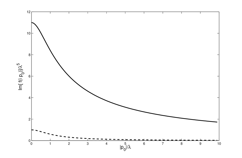
Figure 1: ${\rm Im}[{\tilde{f}_{t}(ip_{0})}]/{\lambda}^{5}$ divided by the TE-perfect conductor result, as a function of $|p_{0}|/\lambda$ for a rigid motion in a medium with constant $g_{t}=\lambda$ in the dashed line. The solid line plot is the ${\rm Im}[{\tilde{f}_{l}(ip_{0})}]/{\lambda}^{5}$ divided by the TE-perfect conductor result, as a function of $|p_{0}|/\lambda$. While dashed line coincides with the TE perfect conductor result for small $|p_{0}|/\lambda$, the solid line goes to 11, which is the correct limit paulo94 .

In Fig. 1 we plot the imaginary part ${\rm Im}\Big{[}{\tilde{f}}(ip_{0})\Big{]}$ divided by the TE-perfect conductor result, as a function of the external frequency. Solid line represents the result of Eq.(45) that, in the limit of $|p_{0}|/\lambda\rightarrow 0$, goes to 11, as it is remarked in Ref.paulo94 . Dashed line corresponds to Eq.(51) and it approaches to 1 in the zero frequency limit (coincides with the perfect conductor limit for the TE mode). Dissipative effects grow with $p_{0}$.

III.3 Evaluation of $\tilde{f}(p_{\parallel})$ for graphene

For the case of graphene, we may apply the tools introduced in the previous section to decompose the vacuum polarization tensor in terms of the irreducible projectors:

$$\widetilde{\Pi}_{\alpha\beta}(k)=\frac{e^{2}N|m|}{4\pi}F\big{(}\frac{k_{0}^{2}+v_{F}^{2}{\mathbf{k}}^{2}}{4m^{2}}\big{)}\Big{[}{\mathcal{P}}^{t}_{\alpha\beta}+\frac{k_{0}^{2}+{\mathbf{k}}^{2}}{k_{0}^{2}+v_{F}^{2}{\mathbf{k}}^{2}}{\mathcal{P}}^{l}_{\alpha\beta}\Big{]}$$ (54)

where:

$$F(x)\;=\;1-\frac{1-x}{\sqrt{x}}\,\arcsin[(1+x^{-1})^{-\frac{1}{2}}]\;,$$ (55)

$m$ is the mass (gap), $N$ the number of $2$-component Dirac fermion fields, and $v_{F}$ the Fermi velocity (in units where $c=1$).

Usually, the most relevant case corresponds to $m=0$; when that is the case:

$$\widetilde{\Pi}_{\alpha\beta} = \frac{e^{2}N}{16}\,\sqrt{k_{0}^{2}+v_{F}^{2}{\mathbf{k}}^{2}}\;\Big{[}{\mathcal{P}}^{t}_{\alpha\beta}\,+\,\frac{k_{0}^{2}+{\mathbf{k}}^{2}}{k_{0}^{2}+v_{F}^{2}{\mathbf{k}}^{2}}{\mathcal{P}}^{l}_{\alpha\beta}\Big{]}$$ (56)

$$= \frac{e^{2}N}{16}\,\sqrt{k_{0}^{2}+{\mathbf{k}}^{2}}\,\Big{[}\,\sqrt{\frac{k_{0}^{2}+v_{F}^{2}{\mathbf{k}}^{2}}{k_{0}^{2}+{\mathbf{k}}^{2}}}\;{\mathcal{P}}^{t}_{\alpha\beta}$$

$$+ \sqrt{\frac{k_{0}^{2}+{\mathbf{k}}^{2}}{k_{0}^{2}+v_{F}^{2}{\mathbf{k}}^{2}}}\;{\mathcal{P}}^{l}_{\alpha\beta}\Big{]}\;.$$

Then, coming back to the general formulae, we see that (with massless fermions), the reflection coefficients are

$$r_{t}(k_{\parallel})\,=\,\frac{1}{1+\frac{32}{e^{2}N}\sqrt{\frac{k_{0}^{2}+{\mathbf{k}_{\parallel}}^{2}}{k_{0}^{2}+v_{F}^{2}{\mathbf{k}_{\parallel}}^{2}}}}$$ (57)

and

$$r_{l}(k_{\parallel})\,=\,\frac{1}{1+\frac{32}{e^{2}N}\sqrt{\frac{k_{0}^{2}+v_{F}^{2}{\mathbf{k}_{\parallel}}^{2}}{k_{0}^{2}+{\mathbf{k}_{\parallel}}^{2}}}}\;.$$ (58)

As there are no dimensionful constants in the VPT, dimensional analysis implies that

$${\tilde{f}}(p_{0})\;=\;|p_{0}|^{5}C(Ne^{2},v_{F})\,,$$ (59)

that is, the result is proportional to that of a perfect conductor. The dimensionless function $C$ depends on the coupling constant and the Fermi velocity.

In order to compute explicitly this function, we insert the graphene reflection coefficients into Eqs.(31) and (32), subtract the Taylor expansion up to order $p_{0}^{4}$, and evaluate the integrals using spherical coordinates. Unlike the previous examples, the complicated dependence of the reflection coefficients with the angle $\theta$ makes not possible to compute analytically this integral. Therefore we computed the form factors numerically for different values of the coupling constants and Fermi velocity. The results are shown in Fig. 2. As expected, the form factors tend to the perfect conductor limit $C\to-1/(30\pi^{2})$ as $Ne^{2}\to\infty$, and vanish in the weak coupling limit $Ne^{2}\to\ 0$. Note that, for small values of the Fermi velocity, the behaviour is non-monotonous with the coupling constant. Most notably, for some values of the parameters, the dissipative effects can be larger for graphene than for perfect conductors.

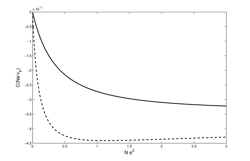
Figure 2: $C(Ne^{2},v_{F})$ as a function of the dimensionless coupling constant $Ne^{2}$ for two different Fermi velocities $v_{F}=0.5$ in the solid line plot, and $v_{F}=0.05$ for the dashed line (in units in which $c=1$). The form factors vanish in the weak coupling limit $Ne^{2}\to\ 0$, and tend slowly to the perfect conductor limit $-1/(30\pi^{2})$ as $Ne^{2}\to\infty$

In the particular case $v_{F}\to 1$, relativistic fermion limit, the reflection coefficients become constants, and the results for the TE and TM form factors are those of the perfect conductor divided by the factor $1+32/(e^{2}N)$.

We end this section pointing out that it would be interesting to compute the VPT in the framework of quantum fields in curved spaces, beyond the weak field approximation, and check explicitly the validity of the approximation $\Pi^{\alpha\beta}_{g}\simeq\Pi^{\alpha\beta}$ used in Eq.(8).

IV Conclusions

We have obtained a general expression for the effective action corresponding to a single imperfect mirror coupled to the EM field, to second order in the departure of the mirror from its equilibrium position. The resulting formula decomposes into two scalar like contributions, in terms of two scalar functions that define the VPT. The final expression for the effective action can be written in a very compact way in terms of the TE and TM reflection coefficients of the mirror. These results can be considered as a generalization to the electromagnetic case of those in Ref.prd07 , where we considered scalar and spinorial vacuum fields and modeled the interaction between an imperfect mirror and the vacuum field using a $\delta$-potential.

We have evaluated explicitly the effective action for some examples, which in our context correspond to the use of the corresponding VPT. We have obtained the vacuum decay amplitude using a proper analytic continuation of the Euclidean results.

We have shown that our results reproduce correctly the TE and TM contributions in the case of perfect conductors. For the particular case of graphene, we have shown that the imaginary part of the effective action is that of a perfect conductor times a function that depends on the coupling constant and the Fermi velocity. We computed explicitly this function and found a non-monotonous behavior with the coupling constant. Moreover, for some values of the parameters, the dissipative effects may be larger than those for a perfect conductor.

It would be of interest to compute the VPT beyond the weak field approximation, in particular for the case of massless fermions. We hope to address this relevant issue in a forthcoming work. This kind of system would require a fuller knowledge of the dependence of the VPT on the geometry. Even in the absence of coupling to the gauge field, a curved monolayer graphene can be considered as a physical realization of quantum field theory in curved spacetimes Iorio , providing condensed matter analogues of semiclassical gravitational effects.

References

- (1) G. T. Moore, J. Math Phys 11, 2679 (1970); S.A. Fulling and P.C.W. Davies, Proc. R. Soc. Lond. A 348, 393 (1976).
- (2) For recent reviews see The nonstationary Casimir effect and quantum systems with moving boundaries, G. Barton, V.V. Dodonov and V.I. Manko (editors), J. Opt. B: Quantum Semiclass. Opt.7 S1 (2005). V. V. Dodonov, Phys. Scripta 82 (2010) 038105; D. A. R. Dalvit, P. A. Maia Neto and F. D. Mazzitelli, Lect. Notes Phys. 834 (2011) 419; P. D. Nation, J. R. Johansson, M. P. Blencowe and F. Nori, Rev. Mod. Phys. 84, 1 (2012).
- (3) C. D. Fosco, F. C. Lombardo and F. D. Mazzitelli, Phys. Rev. D 76, 085007 (2007).
- (4) C. D. Fosco, F. C. Lombardo and F. D. Mazzitelli, Phys. Rev. D 84, 025011 (2011).
- (5) R. Golestanian and M. Kardar, Phys. Rev. A 58, 1713 (1998).
- (6) M. F. Maghrebi, R. Golestanian and M. Kardar, Phys. Rev. D 87, 025016 (2013).
- (7) A. O. Barvinsky and G. A. Vilkovisky, Nucl. Phys. B 333, 512 (1990), and references therein.
- (8) I. V. Fialkovsky, V. N. Marachevsky and D. V. Vassilevich, Phys. Rev. B 84, 035446 (2011).
- (9) More generally, is the total vacuum decay probability, which also includes the possibility of excitation of the internal degrees of freedom of the mirror. These internal degrees of freedom also produce inertial forces and dissipation on the accelerated mirror, see for instance Ref.inertial .
- (10) C. D. Fosco, F. C. Lombardo and F. D. Mazzitelli, Phys. Rev. D 82, 125039 (2010).
- (11) We computed the integrals using Mathematica. A useful point is to note that, after the integration in , the resulting function vanishes for .
- (12) P. A. Maia Neto, J. Phys. A: Math. Gen. 27, 2167 (1994).
- (13) M. Bordag, Phys. Rev. D 70, 085010 (2004).
- (14) K. A. Milton and J. Wagner, J. Phys. A 41, 155402 (2008).
- (15) A. Iorio and G. Lambiase, arXiv:1308.0265 [hep-th].