A minimal model for acoustic forces on Brownian particles

Abstract

We present a generalization of the inertial coupling (IC) [Usabiaga et al. J. Comp. Phys. 2013] which permits the resolution of radiation forces on small particles with arbitrary acoustic contrast factor. The IC method is based on a Eulerian-Lagrangian approach: particles move in continuum space while the fluid equations are solved in a regular mesh (here we use the finite volume method). Thermal fluctuations in the fluid stress, important below the micron scale, are also taken into account following the Landau-Lifshitz fluid description. Each particle is described by a minimal cost resolution which consists on a single small kernel (bell-shaped function) concomitant to the particle. The main role of the particle kernel is to interpolate fluid properties and spread particle forces. Here, we extend the kernel functionality to allow for an arbitrary particle compressibility. The particle-fluid force is obtained from an imposed “no-slip” constraint which enforces similar particle and kernel fluid velocities. This coupling is instantaneous and permits to capture the fast, non-linear effects underlying the radiation forces on particles. Acoustic forces arise either because an excess in particle compressibility (monopolar term) or in mass (dipolar contribution) over the fluid values. Comparison with theoretical expressions show that the present generalization of the IC method correctly reproduces both contributions. Due to its low computational cost, the present method allows for simulations with many [$O(10^{4})$] particles using a standard Graphical Processor Unit (GPU).

I Introduction

Sound waves in the ultrasonic frequency range $\omega>\mathrm{kHz}$, are used for an amazing list of applications such as object detection, testing flaws in materials, medical imaging, cleaning, therapeutic al purposes, tumor destruction, and even as weapon. A related phenomena, cavitation, uses powerful kHz waves to produce a significant temperature and pressure increase in the liquid and locally boost chemical reactions. At larger MHz frequencies, the sound wavelength in a typical liquid is in the millimeter range and thus suited for lab-on-a-chip technologies Settnes and Bruus (2012). MHz sound interacts and impinges forces to micron-size particles due to a nice example of non-linear correlation between the oscillating density and velocity fields Settnes and Bruus (2012). Such force, known as acoustic radiation force Settnes and Bruus (2012), was theoretically predicted for rigid objects in a fluid by King King (1934) in 1934 and two decades later extended to compressible particles by Yoshioka and KawashimaYosioka and Kawasima (1955). In the sixties, Gor’kov Gorkov (1962) published an elegant approach in the soviet literature, showing that in the inviscid limit (large enough frequencies) the radiation force for standing waves can be derived from the gradient of an effective potential energy ${\boldsymbol{F}}_{ac}=-\nabla U_{ac}$; a result that has been quite useful for subsequent engineering applications. The (sometimes called Wang and Dual (2011)) Gor’kov potential, scales with the particle volume $\mathbb{V}$ and has contributions from the time-averaged pressure $p_{in}$ and velocity $v_{in}$ of the incoming wave,

$$U_{ac}=-\frac{\mathbb{V}}{2}\left[\kappa_{e}\langle p_{in}^{2}\rangle+\frac{3m_{e}}{2m_{p}+\rho_{0}\mathbb{V}}\rho_{0}\langle v_{in}^{2}\rangle\right],$$ (1)

where $\rho_{0}$ is the fluid density and $\langle x\rangle=(1/\tau)\int_{0}^{\tau}x(t)dt$ and $\tau=2\pi/\omega$ is the oscillation period. These two contributions to the acoustic potential (1) are proportional to particle excess-quantities relative to the fluid values. In particular, $m_{e}=m_{p}-\rho_{0}\mathbb{V}$ denotes the excess of particle mass ($m_{p}$) over the mass of fluid it displaces $\rho_{0}\mathbb{V}$ and $\kappa_{e}=\kappa_{p}-\kappa_{f}$ is the excess in particle compressibility ($\kappa=(1/\rho)\partial\rho/\partial p$) relative to the fluid. Despite their relevance, the early papers on acoustic radiation were rather scarce in explanations and recent theoretical works revisiting this phenomenon have been most welcome (see Settnes and Bruus (2012) and citations thereby). Bruus Settnes and Bruus (2012) used a perturbation expansion in the (small) wave amplitude to show that both terms in Eq. 1 are in fact related to the monopole and dipolar moments of the flow potential, which are uncoupled in linear acoustics. He also extended the analysis to the viscid regime (smaller frequencies) generalizing previous studied by Doinikov Doinikov (1994, 1997) and others (see Settnes and Bruus (2012)).

The first application of ultrasound forces were carried out in the eighties by Maluta et al. Dion et al. (1982). They used standing waves to trap and orient wood pulp fibers diluted in water into the equidistant pressure planes. The idea was used by the paper industry to measure the fiber size. Recently the usage of ultrasound for manipulation of small objects is flourishing and offering many promising applications for material science, biology, physics, chemistry and nanotechnology. An excellent review of the current state-of-art can be found in the monographic issue on the journal Lab on a chip [Volume 12, (2012)] and also in the review of Ref. Friend and Yeo (2011) which focuses on applications, cavitation and more exotic phenomena. Trapping extremely small objects (reaching submicron-sizes) using ultrasound, in what has been called “acoustic tweezers” Ding et al. (2012), is explored by several groups Oberti et al. (2007); Ding et al. (2012) and used for many different purposes, such as to move and capture colloids Oberti et al. (2007) or even individual living cells without even damaging themHaake et al. (2005); Ding et al. (2012). Quoting T.J.Huang: “acoustic tweezers are much smaller than optical tweezers and use 500,000 times less energy.”Ding et al. (2012)

Despite the increase in theoretical and experimental works, there are not too many numerical simulations on ultrasound-particle interaction. Its cause might be the inherent difficulties this phenomenon poses to numerical calculations. The acoustic force arises as a non-linear coupling between two fast-oscillating signals and only manifests after averaging over many oscillations. This means a tight connection between the fastest hydrodynamic mode (sound) and the much slower viscous motion of the particle, at a limiting velocity dictated by the viscous drag. The situation, from the numerical standpoint, is even worse if one is interested in studying the dispersion of many small colloids around the loci of the minima of the Gor’kov potential, because dispersion is a diffusion-driven process and requires much longer time scales. Colloidal dispersion around the accumulation loci is certainly important and a nuisance for many applications. It was first studied by Higashitani et al Higashitani et al. (1981), who worked with the hypothesis that the particles follow a Boltzmann distribution based on the acoustic potential energy. Simulation of a swarm of particles diffusing under acoustic radiation involve solving an intertwined set of mechanisms acting over time-scales spanning over many decades. As a typical example, in a liquid, sound crosses a micron-size colloid in $R/c_{F}\sim 10^{-9}$ seconds, while the colloid diffuses its own radius in $R^{2}/D\sim 10^{0}$ seconds. Such wide dynamic range is certainly impossible to tackle for any numerical method involving a detailed resolution of each particle surface.

An important task for numerical studies in the realm of acoustic force applications is the determination of the pressure pattern in resonant cavities Skafte-Pedersen (2008); Dual et al. (2012). The main objective of these calculations, which solve the Helmholtz wave equation (but do not involve any particle) is to forecast the pressure nodes inside the chamber, where colloidal coagulation is expected to occur. Using a one-way-coupling approach Maxey and Riley (1983), it is also possible to get some insight on the particle trajectories, by directly applying the theoretical acoustic forces together with the (self-particle) viscous drag Muller et al. (2012). This leads however to uncontrolled approximations Skafte-Pedersen (2008) which neglect significant non-linear effects such as the hydrodynamic particle-particle interactions and the effect of multiple particle scattering on the wave pattern Feuillade (1996).

Another group of numerical studies explicitly calculate the acoustic force on objects although, to the best of our knowledge, have been so far restricted to single two-dimensional spheres (or, more precisely axially projected ”cylinders”) Wang and Dual (2009). These works were based on finite element or finite volume discretizations of the fluid and the immersed object, with explicit resolution of its surface (no-slip and impenetrability conditions). The effect of viscous loss has been studied in a recent work Wang and Dual (2011). There are also some calculations using Lattice Boltzmann solvers Barrios and Rechtman (2008) also involving single 2D cylinders and ideal fluid. It has to be mentioned that all these works considered rigid particles. In fact, implementing a finite particle compressibility is not straightforward for this type of surface-resolved approach as it would demand implementing elastic properties to the solid and couple it to the dynamics of the particle interiorHasegawa (1979). Another downside of fully fledged resolution is the large computational cost per particle which limits feasible simulations to few particles at most.

In this work we propose a quite different modeling route for the particle dynamics. First, our method is based on the Eulerian-Lagrangian approach Dünweg and Ladd (2009); Peskin (2002), meaning that particles are not constructed with or restricted to the “fluid mesh” but move freely in the continuum space. This avoids complicated triangulation and remeshing around the particle and permits solve the fluid equations (we consider Navier-Stokes Fluctuating Hydrodynamics) in a simple regular lattice of fluid cells, using a finite volume scheme Balboa Usabiaga et al. (2012a). Second, particles are described with a minimal-resolution model involving a single kernel function per particle, which just contains $3^{3}$ fluid-cells in 3D. The particle kernel, originally designed by Peskin and Roma Roma et al. (1999) for the Immersed Boundary (IB) method, is used to interpolate local fluid properties and to spread the particle forces to the surrounding fluid. The third important issue, and in fact the novelty of what we refer to as “inertial coupling” (IC) method Balboa Usabiaga et al. (2013) resides in imposing an instantaneous “no-slip” constraint (the particle velocity equals the interpolated fluid velocity) to couple the dynamics of the particle and the fluid. Such coupling is instantaneous and, as shown in our previous work Balboa Usabiaga et al. (2013) it captures the fast ultrasound-particle interaction. Here we further explore this line of minimally-resolved particle modeling which is based on the idea that the particle kernel (originally designed for interpolation purposes Peskin (2002)) can be used to embed all the relevant physical properties of the particle, such as its hydrodynamic radius $R_{H}$ Dünweg and Ladd (2009), its volume $\mathbb{V}$, and mass ($m_{p}=m_{e}+\rho_{\mathbb{V}}$). A characteristic feature of this minimal model (which proves to be beneficial for the present work) is the absence of density boundary conditions to ensure the particle impenetrability across its surface. In fact, in the present model the “particle” has not a well-defined surface and the fluid density field is not zero inside the particle domain. For this reason, after Dunweg and Ladd Dünweg and Ladd (2009), this model is sometimes called “blob” model. Imposing a pressure force ${\boldsymbol{F}}$ to a surface-less “particle” is however not a problem provided it is contained in a well defined volume $\mathbb{V}$. Thanks to Gauss-Ostrogradsky integral theorem, we can convert the traction done by pressure (tensor) ${\bf P}$ over the particle surface $S$ to an integral over its volume $\mathbb{V}$

$${\boldsymbol{F}}=-\oint_{S}{\bf P}\cdot{\boldsymbol{n}}\,\mathrm{d}r^{2}=-\int_{\mathbb{V}}\nabla\cdot{\bf P}\mathrm{d}r^{3}=-\mathbb{V}\int\Theta({\bf q}-{\boldsymbol{r}})\nabla\cdot{\bf P}\mathrm{d}r^{3}.$$ (2)

where ${\bf q}$ is the position of the particle center. The second equality is indeed exact for the hard-kernel of a rigid particle $\Theta(\boldsymbol{q}-{\boldsymbol{r}})$ which differs from zero only inside the particle, where

$$\Theta({\bf q}-{\boldsymbol{r}})=1/\mathbb{V}\;\;\mbox{for}|{\boldsymbol{r}}-\boldsymbol{q}|<a.$$ (3)

The “blob” approach consist on deploying instead a soft-kernel (bell-shape, everywhere derivable). Slightly different version of this idea is used in all Eulerian-Langrangian and fully Lagrangian (meshfree) particle methods Lomholt and Maxey (2003); Tatsumi and Yamamoto (2012); Vazquez-Quesada et al. (2012).

The IC method for particle hydrodynamics was presented in a recent work Balboa Usabiaga et al. (2013) and subsequently extended to incompressible flow Balboa Usabiaga et al. (2012b). Capturing ultrasound forces was one of the relevant tests performed Balboa Usabiaga et al. (2013) to check the viability of its instantaneous coupling. However, as stated, the original blob model does not impose any constraint on the fluid density field and, not unexpectedly, the resulting acoustic forces were found to be fully compatible with particles with the same compressibility than the fluid, i.e. to $\kappa_{e}=\kappa_{p}-\kappa_{f}=0$. Inspection of Eq. (1) indicates that our neutrally buoyant “blobs” $m_{e}=0$ did not experienced any irradiation force. In the present work we focus on the acoustic force problem and extend the blob model to allow for a particle compressibility, different from that of the fluid. This is part of a research line with two main targets: to extend the kernel functionality by assigning more physical properties to it and more generally, to highlight that a carefully built minimally-resolved model can achieve considerable accuracy and capture realistic physics over a broader range of time and length scales.

We start by presenting the essential kernel properties in Section II and focus in how to implement the particle compressibility in Sec. III. The dynamics of the particle and fluid coupled equations of motion is described in Sec. IV, where it is shown that the model preserves the local momentum and also the energy in the ideal fluid limit. It is then shown that equilibrium fluctuations (of velocity and particle density) are consistent with the thermodynamic prescriptions. Acoustic forces are briefly reviewed in Sec. V. Simulations, presented in Sec. VI, are shown to agree with the theoretical monopolar and dipolar primary forces. A study of the dispersion of a small colloid under a standing wave is also presented. Concluding remarks are finally given in Sec. VII.

II Particle model: kernel properties

One of the most important issues in the blob-particle approach is the construction of the particle kernel $\theta_{h}({\boldsymbol{r}}-\boldsymbol{q})$. From the standpoint of the hybrid Eulerian-Lagrangian methodology, the role of the kernel is to act as the “glue” between both descriptions. As carefully explained in previous works Balboa Usabiaga et al. (2012b); Atzberger (2011), the kernel provides the two translating operations: the averaging operator transfers information from the Eulerian representation of the fluid to the Lagrangian representation of the particles $\boldsymbol{J}:\mathcal{E}\rightarrow\mathcal{L}$ while the the spreading operator $\boldsymbol{S}:\mathcal{L}\rightarrow\mathcal{E}$, translates “Lagrangian” forces into “Eulerian” force density fields.

In the continuum formulation, these two operations are defined as

$$\boldsymbol{J}(\boldsymbol{q}){\boldsymbol{v}}({\boldsymbol{r}}) = \int\theta_{h}(\boldsymbol{q}-{\boldsymbol{r}}){\boldsymbol{v}}({\boldsymbol{r}})\;d^{3}r,$$ (4)

$$\boldsymbol{S}(\boldsymbol{q}){\boldsymbol{F}}(\boldsymbol{q}) = \theta_{h}(\boldsymbol{q}-{\boldsymbol{r}}){\boldsymbol{F}}(\boldsymbol{q}),$$ (5)

so it is clear that $\boldsymbol{S}$ has units of inverse volume. As noted in Balboa Usabiaga et al. (2012b), using the same kernel to spread and interpolate, brings about an important mathematical property which is crucial to maintain energy conservation and the fluctuation dissipation balance: $\boldsymbol{J}$ and $\boldsymbol{S}$ are adjoint,

$$\boldsymbol{J}{\boldsymbol{v}}\cdot{\boldsymbol{u}}=\int{\boldsymbol{v}}\cdot\boldsymbol{S}{\boldsymbol{u}}\,d^{3}r=\int\theta_{h}(\boldsymbol{q}-{\boldsymbol{r}}){\boldsymbol{v}}\cdot{\boldsymbol{u}}d^{3}r$$ (6)

The Eulerian fluid description is solved in a discrete mesh, which for practical purposes is regular, ${\boldsymbol{r}}_{\vec{k}}=h{\vec{k}}$. Therefore, in practice, one needs to work with the discrete version of Eqs. 4,

$$\boldsymbol{J}(\boldsymbol{q}){\boldsymbol{v}}({\boldsymbol{r}}) = \sum_{i}h^{3}\theta_{h}(\boldsymbol{q}-{\boldsymbol{r}}_{i}){\boldsymbol{v}}({\boldsymbol{r}}_{i})$$ (7)

$$\boldsymbol{S}(\boldsymbol{q}-{\boldsymbol{r}}_{i}){\boldsymbol{F}}(\boldsymbol{q}) = \theta_{h}(\boldsymbol{q}-{\boldsymbol{r}}_{i}){\boldsymbol{F}}(\boldsymbol{q})$$ (8)

where $h^{3}$ is the volume of the hydrodynamic cell. Discreteness brings about restrictions in the kernel shape. First, the operation $\boldsymbol{J}$ becomes a discrete average which should at least have linear consistency: i.e. for any Lagrangian position $\boldsymbol{q}$,

$$\sum_{i}h^{3}\theta_{h}({\boldsymbol{r}}_{i}-\boldsymbol{q}) = 1$$ (9)

$$\sum_{i}h^{3}({\boldsymbol{r}}_{i}-\boldsymbol{q})\theta_{h}({\boldsymbol{r}}_{i}-\boldsymbol{q}) = 0.$$ (10)

This ensures that any linear field $f(r)=a+br$ is exactly interpolated, $f(q)=\sum_{i}h^{3}f(r_{i})\theta_{h}(r_{i}-q)$.

II.1 Kernel volume

In the blob-model approach, the particle kernel is not only sought as mathematical object, but also a tool to provide physical meaning to the particle model. This idea is clearly illustrated with the kernel volume, which in fact, introduces the third condition in the kernel construction. Note that the norm of the hard-kernel (3) trivially yields the inverse volume of the domain, $\int\Theta({\bf q}-{\boldsymbol{r}})^{2}d^{3}r=1/\mathbb{V}$. Similarly, in the discrete Eulerian mesh, the norm of the kernel,

$$\boldsymbol{J}\boldsymbol{S}=\sum_{i}h^{3}\theta_{h}({\boldsymbol{r}}_{i}-\boldsymbol{q})^{2}=1/\mathbb{V},$$ (11)

should be independent on the Lagrangian position $\boldsymbol{q}$. Although for different reasons, this condition (11) was first formulated by Peskin Peskin (2002) in his Immersed Boundary (IB) method. In fact, conditions (9),(10) and (11) determine the 3-point kernel introduced by Roma and Peskin Roma et al. (1999), whose norm, in 1D, is $(1/2)h$. For 3D, the standard tensor product construction, $\theta_{h}({\boldsymbol{r}})=\theta_{h}(x)\theta_{h}(y)\theta_{h}(z)$, which trivially yields, $\mathbb{V}=8h^{3}$. Thus, the “blob” volume cannot be arbitrary changed, being a property of the kernel.

II.2 Hydrodynamic radius

The kernel provides all the relevant physical dimensions of the “blob”. In previous works Balboa Usabiaga et al. (2012b); Balboa Usabiaga et al. (2013) we measured its hydrodynamic radius [$R_{H}=(0.91\pm 0.01)\,h$, where the error bar comes from the variation of $R_{H}$ over the mesh] from the ratio between a drag force $F_{d}$ and the resulting fluid terminal velocity $v_{0}$, at small Reynolds number, $R_{H}=F_{d}/(6\pi\eta v_{0})$. Fitting the perturbative flow created around the blob to the Stokes profile gave a similar value of $R_{H}$ Balboa Usabiaga et al. (2013). The size of the perturbative vorticity field created by the particle is related to its hydrodynamic radius and can be also estimated from its effective Faxén radius. The perturbative velocity field ${\boldsymbol{v}}(r)$ created by an immersed sphere at ${\boldsymbol{r}}=\boldsymbol{q}$ can be expanded as ${\boldsymbol{v}}({\boldsymbol{r}})={\boldsymbol{v}}(\boldsymbol{q})+(a^{2}/6)\nabla^{2}{\boldsymbol{v}}(\boldsymbol{q})+...$ Kim and Karrila (1991). The Faxén term is proportional to the squared particle radius $a^{2}$. Taylor expanding ${\boldsymbol{v}}(r)$ around $\boldsymbol{q}$,

$${\boldsymbol{v}}({\boldsymbol{r}})={\boldsymbol{v}}(\boldsymbol{q})+\nabla{\boldsymbol{v}}(\boldsymbol{q})({\boldsymbol{r}}-\boldsymbol{q})+\frac{1}{2}({\boldsymbol{r}}-\boldsymbol{q})^{T}\cdot\nabla\nabla{\boldsymbol{v}}(\boldsymbol{q})\cdot({\boldsymbol{r}}-\boldsymbol{q})+...$$ (12)

and applying the average operator $\boldsymbol{J}$ yields,

$$\boldsymbol{J}{\boldsymbol{v}}({\boldsymbol{r}})={\boldsymbol{v}}(\boldsymbol{q})+\frac{1}{2}\nabla^{2}{\boldsymbol{v}}(\boldsymbol{q})\boldsymbol{J}\left[(r-q)^{2}\right]+O(\boldsymbol{J}\left[(r-q)^{4}\right]),$$ (13)

which informs about the effective Faxén radius of our blob model Balboa Usabiaga et al. (2012b): $R_{F}^{2}=3\boldsymbol{J}\left[(r-q)^{2}\right]$. For the 3-pt kernel this gives $R_{F}=0.945\,h$ with a small variation of about $5\%$ over the mesh.

III Blob compressibility

In this work the idea of adding physical properties to the blob, via the kernel, is extended to provide a finite blob compressibility. To that end we use the kernel to include a local particle contribution to the pressure equation of state. The idea is thus quite general and independent of the type of particle-fluid coupling used and of the equations of motion (presented in Sec. IV), although here we solve the isothermal compressible Navier-Stokes equations. The pressure of the fluid phase is barotropic $p=p(\rho)$ and we consider $p(\rho)=p_{0}+c_{f}^{2}\rho$, with constant speed of sound $c_{f}$. To take into account the effect of a compressible particle in the fluid we propose a modification to the pressure field based on the following functional,

$$\pi(\rho,\boldsymbol{q})=p(\rho)+\boldsymbol{S}(\boldsymbol{q})\Omega(\rho;\boldsymbol{q}).$$ (14)

The extra particle contribution $\boldsymbol{S}(\boldsymbol{q}-{\bf r})\Omega(\rho;\boldsymbol{q})$ only affects locally within each particle domain. Recall that $\boldsymbol{S}$ has units of inverse volume, so $\Omega$ has dimensions of energy. In fact, the field $\boldsymbol{S}\Omega$ can be related to the chemical potential created by particle-fluid interactions Español and Delgado-Buscalioni (2013) (see Sec.VII). It determines the energetic cost for fluid entertainment into the kernel domain. A simple, yet efficient, implementation of $\Omega$ consists on assuming that the particle contribution to the pressure is a linear function of the averaged local density,

$$\Omega(\boldsymbol{J}\rho)=\epsilon_{pf}\mathbb{V}\left(\boldsymbol{J}\rho-\rho_{0}\right)$$ (15)

where $\rho_{0}$ is the fluid equilibrium density and the auxiliary parameter $\epsilon_{pf}$ is the particle-fluid interaction energy per unit of fluid mass Español and Delgado-Buscalioni (2013). Note that $\Omega$ depends on $\boldsymbol{q}$ through the average operator $\boldsymbol{J}=\boldsymbol{J}(\boldsymbol{q})$. A variation in $\Omega$ corresponds to a work done by the fluid to compress the particle domain, or more precisely to increase the fluid density inside the fixed volume $\mathbb{V}$ (which surrounds the particle and moves along with it). The particle mass can assigned to be $m_{p}=m_{e}+\rho_{0}\mathbb{V}$, where $m_{e}$ is the excess of particle mass over the mass of fluid it displaces in equilibrium ($\Omega=0$). Thus, in Eq. (15) we choose $\Omega$ to be proportional to the mass of fluid $\mathbb{V}(\boldsymbol{J}\rho-\rho_{0})$ that have entered into the kernel domain. The resulting fluid work is positive if the particle is compressed and viceversa. We will come back to this issue in next section where the equation of motion of the blob is derived.

One can now evaluate the compressibility $\kappa({\boldsymbol{r}})$ and the speed of sound $c({\boldsymbol{r}})$ of the fluid, which are scalar fields. To that end we evaluate the pressure variation $\delta\pi({\boldsymbol{r}})$

$$\delta\pi({\boldsymbol{r}})=\int\frac{\delta\pi({\boldsymbol{r}})}{\delta\rho({\boldsymbol{r}}^{\prime})}\delta\rho({\boldsymbol{r}}^{\prime})d^{3}r$$ (16)

where the functional derivative $\delta\pi({\boldsymbol{r}})/\delta\rho({\boldsymbol{r}}^{\prime})$ provides change of the pressure field at ${\boldsymbol{r}}$ (per unit volume) due to a density perturbation $\delta\rho({\boldsymbol{r}}^{\prime})$. The total pressure functional can be written as

$$\pi({\boldsymbol{r}})=\int p[\rho({\boldsymbol{r}}^{\prime})]\delta({\boldsymbol{r}}^{\prime}-{\boldsymbol{r}})d^{3}r^{\prime}+\epsilon_{pf}\mathbb{V}\theta_{h}(\boldsymbol{q}-{\boldsymbol{r}})\int\theta_{h}(\boldsymbol{q}-{\boldsymbol{r}}^{\prime})(\rho({\boldsymbol{r}}^{\prime})-\rho_{0})d^{3}r^{\prime},$$ (17)

whose functional derivative is given by

$$\frac{\delta\pi({\boldsymbol{r}})}{\delta\rho({\boldsymbol{r}}^{\prime})}=c_{f}^{2}\delta({\boldsymbol{r}}-{\boldsymbol{r}}^{\prime})+\epsilon_{pf}\mathbb{V}\theta_{h}(\boldsymbol{q}-{\boldsymbol{r}})\theta_{h}(\boldsymbol{q}-{\boldsymbol{r}}^{\prime}).$$ (18)

where, $c_{f}$ is constant for the fluid equation of state used hereby (in general $c_{f}^{2}({\boldsymbol{r}})=\partial p(\rho({\boldsymbol{r}}))/\partial\rho$ is a density dependent field).

In terms of the spreading and average operators, the pressure first variation is then

$$\delta\pi({\boldsymbol{r}})=c_{f}^{2}\delta\rho({\boldsymbol{r}})+\epsilon_{pf}\mathbb{V}\boldsymbol{S}\boldsymbol{J}(\delta\rho).$$ (19)

A sound velocity field $c({\boldsymbol{r}})$ can be defined as

$$c^{2}({\boldsymbol{r}}) = \int\frac{\delta\pi({\boldsymbol{r}})}{\delta\rho({\boldsymbol{r}}^{\prime})}d^{3}r^{\prime}=c_{f}^{2}+\epsilon_{pf}\mathbb{V}\boldsymbol{S}(\boldsymbol{q}-{\boldsymbol{r}})$$ (20)

Averaging in (19) gives the overall variation of pressure inside the kernel which, for constant fluid sound velocity $c_{f}$ is equal to,

$$\boldsymbol{J}[\delta\pi]=\left(c_{f}^{2}+\epsilon_{pf}\right)\boldsymbol{J}[\delta\rho],$$ (21)

where we have used $\boldsymbol{J}\boldsymbol{S}=\mathbb{V}^{-1}$. Equation (21) can be understood as the blob equation of state, which justify our identification of $c_{p}$ with the speed of sound inside the particle. It is given by,

$$c_{p}=\sqrt{c_{f}^{2}+\epsilon_{pf}}.$$ (22)

The input parameter $\epsilon_{pf}$ can be then either positive or negative (with the obvious condition $c_{p}\geq 0$). For instance, taking $\epsilon_{pf}\simeq-c_{f}^{2}$ permits to simulate very compressible particles (gas bubbles). Equivalently, one can introduce $\kappa_{p}=\kappa_{f}+\kappa_{e}$ where $\kappa_{p}\equiv 1/(\rho_{0}c_{p}^{2})$ and $\kappa_{f}=1/(\rho_{0}c_{f}^{2})$ provide the particle and fluid compressibility, respectively. Then using (22), the “excess particle compressibility” is just

$$\kappa_{e}=-\frac{\epsilon_{pf}}{c_{p}^{2}}\kappa_{f}.$$ (23)

It is noted that the term related to the particle compressibility in the ultrasound potential of Eq. (1) is proportional to $\kappa_{e}$ but either $\epsilon_{pf}$ or $\kappa_{e}$ can be used as input parameters of the model.

From Eq. (19) one can also infer a bulk modulus operator which applied to any density perturbation field $\delta\rho({\boldsymbol{r}})$ provides the resulting variation in the pressure field $\delta\pi({\boldsymbol{r}})=\mathcal{B}\delta\rho({\boldsymbol{r}})/\rho_{0}$,

$$\rho_{0}^{-1}\mathcal{B}\equiv c_{f}^{2}{\bf 1}+\epsilon_{pf}\mathbb{V}\boldsymbol{S}\boldsymbol{J}$$ (24)

Its inverse ${\boldsymbol{\kappa}}=\mathcal{B}^{-1}$ is the compressibility operator, which applied to some pressure field $\delta\hat{p}({\boldsymbol{r}})$ provides the resulting density perturbation $\delta\hat{\rho}({\boldsymbol{r}})=\rho_{0}{\boldsymbol{\kappa}}[\delta\hat{p}({\boldsymbol{r}})]$. To invert (24) one can use the same formal Taylor expansion used in appendix A of Ref. Balboa Usabiaga et al. (2012b) and get,

$${\boldsymbol{\kappa}}=\kappa_{f}+\kappa_{e}\mathbb{V}\boldsymbol{S}\boldsymbol{J}.$$ (25)

IV Inertial coupling method

IV.1 Coupling

In this section we present the essence of the Inertial Coupling (IC) method Balboa Usabiaga et al. (2013); Balboa Usabiaga et al. (2012b), developed to capture inertial effects in simulation of colloids and other microparticles in compressible or incompressible flows. The IC method uses ingredients of the Immersed Boundary (IB) method Peskin (2002), and in particular those related to how to “hide” the discrete mesh to the kernels. Here however, each kernel is not a surface-marker, but represents a single particle whose dynamics should be infered from some suitable coarse-grained representation of the constraints it imposes to the fluid velocity. In particular, the fluid velocity at the boundary of a spherical particle with a non-slip surface should satisfy,

$${\boldsymbol{v}}({\boldsymbol{r}})={\boldsymbol{u}}+{\boldsymbol{\omega}}\times\left({\boldsymbol{r}}-\boldsymbol{q}\right)\;\;\mbox{for}|{\boldsymbol{r}}-\boldsymbol{q}|\leq a,$$ (26)

where $a$ is the particle radius, ${\boldsymbol{u}}$ its translation velocity, ${\boldsymbol{\omega}}$ its angular velocity and $\boldsymbol{q}$ its center position. Applying the average operator in the previous equation and noting that $\boldsymbol{J}(\boldsymbol{q})[{\boldsymbol{r}}-\boldsymbol{q}]=0$ one gets a coarse-grained representation of the no-slip constraint,

$$\boldsymbol{J}(\boldsymbol{q}){\boldsymbol{v}}({\boldsymbol{r}})={\boldsymbol{u}}.$$ (27)

which is the one implemented in the present method. The constraint (27) does not resolve the effect of particle rotation and rigidity (no strain) on the surrounding fluid (see Refs. Yeo and Maxey (2010) for generalizations). The no-slip constraint is non-dissipative, so it conserves the energy of the fluid-particle system in reversible processes (i.e. in the inviscid limit) Balboa Usabiaga et al. (2012b). The no-slip constraint (27) can be generalized to allow for partial slip (see Appendix B of Balboa Usabiaga et al. (2012b)) which introduces a finite relaxation time ($m/\xi\sim\mu\mathrm{s}$) for the equilibration of the particle and local fluid velocities Bedeaux and Mazur (1974). Partial-slip dissipates energy and requires adding an extra random force to represent the transmission of momentum (tangential to the particle surface) through fluid-particle molecular collisions and to guarantee the fluctuation-dissipation balance. By contrast, the no-slip constraint idealizes instantaneous fluid-particle interactions which, in practice captures the extremely fast forces involved in the acoustic time scale ($a/c\sim 10^{3}\mathrm{ps}$), which are actually not far from molecular forces decorrelation times Kinsler et al. (2000).

IV.2 Dynamics

In this section we present the equations of motion for the fluid and a single particle (the generalization to $N$ particles is straightforward). These equations were discussed in previous works Balboa Usabiaga et al. (2013); Balboa Usabiaga et al. (2012b) and the novelty here is the addition of the particle compressibility contribution in the pressure field $\pi=\pi(\rho,\boldsymbol{q})$, whose details were discussed in Sec. III. The fluid and particle dynamics are specified by the conservation of fluid mass and momentum [Eqs. (28) and (29)], the particle momentum Eq. (30) and the (no-slip) fluid-particle coupling (31),

$$\partial_{t}\rho+\boldsymbol{\nabla}\cdot{\boldsymbol{g}} = 0$$ (28)

$$\partial_{t}{\boldsymbol{g}}+\boldsymbol{\nabla}\cdot({\boldsymbol{g}}{\boldsymbol{v}}) = -\boldsymbol{\nabla}\cdot{\boldsymbol{P}}-\boldsymbol{S}\boldsymbol{\lambda}$$ (29)

$$m_{e}\dot{{\boldsymbol{u}}} = {\boldsymbol{F}}(\boldsymbol{q},t)+\boldsymbol{\lambda}$$ (30)

$$\mbox{s.t. }{\boldsymbol{u}} = \boldsymbol{J}{\boldsymbol{v}}.$$ (31)

The total stress tensor is now given by,

$${\boldsymbol{P}}=\pi{\bf 1}-\boldsymbol{\sigma}=p(\rho){\bf 1}+\boldsymbol{S}(\boldsymbol{q}-{\boldsymbol{r}})\Omega-\boldsymbol{\sigma},$$ (32)

where the particle-fluid interaction energy $\Omega$ is given by Eq. (15). We consider a Newtonian fluid, with constant shear and bulk viscosities $\eta$ and $\zeta$ and this allows us to write the divergence of the viscous terms in the standard Laplacian form,

$$\boldsymbol{\nabla}\cdot\boldsymbol{\sigma}=\eta\boldsymbol{\nabla}^{2}{\boldsymbol{v}}+\left(\zeta+\frac{\eta}{3}\right)\boldsymbol{\nabla}(\boldsymbol{\nabla}\cdot{\boldsymbol{v}})+\boldsymbol{\nabla}\cdot\boldsymbol{\Sigma},$$ (33)

The stochastic components of the stress tensor are collected in $\boldsymbol{\Sigma}$ Landau and Lifshitz (1987); Fabritiis et al. (2007); Donev et al. (2010); Balboa Usabiaga et al. (2012a); Balboa Usabiaga et al. (2013), being given by

$$\boldsymbol{\Sigma}=\sqrt{2\eta k_{B}T}\widetilde{\mathcal{W}}+\left(\sqrt{\frac{\zeta k_{B}T}{3}}-\frac{1}{3}\sqrt{2\eta k_{B}T}\right)\mbox{Tr}\left(\widetilde{\mathcal{W}}\right)\boldsymbol{I}.$$ (34)

Where the symmetric tensor $\widetilde{\mathcal{W}}=(\mathcal{W}+\mathcal{W}^{T})/2$ is defined by the covariance of a random Gaussian tensor $\mathcal{W}$ delta-correlated in time and space,

$$\langle\mathcal{W}_{ij}({\boldsymbol{r}},t)\mathcal{W}_{kl}({\boldsymbol{r}}^{\prime},t^{\prime})\rangle=\delta_{ik}\delta_{jl}\delta({\boldsymbol{r}}-{\boldsymbol{r}}^{\prime})\delta(t-t^{\prime}).$$ (35)

The particle evolves according the Second Newton’s Law (30) and receives the force exerted by the fluid $\boldsymbol{\lambda}$ and eventually some other external (or inter-particle) potential force ${\boldsymbol{F}}(\boldsymbol{q},t)$. In turn, the fluid phase receives back from the particle a local source of momentum density given by $-\boldsymbol{S}\boldsymbol{\lambda}$ (see Eq. 29). This form guarantees the Third Newton’s Law both globally and locally (see Balboa Usabiaga et al. (2012b) and below). In passing we note that, in contrast to friction-based couplings Giupponi et al. (2007); Dünweg and Ladd (2009), we do not assume any functional form for the fluid force $\boldsymbol{\lambda}$. Instead, $\boldsymbol{\lambda}$ is treated as a Lagrangian multiplier to impose (at any instant) the no-slip constraint (31). This allows to recover the correct hydrodynamics under quite different flow regimes; even at large Reynolds numbers where the drag force has a strong convective origin and strongly deviates from the Stokes (friction) value Balboa Usabiaga et al. (2013); Español and Delgado-Buscalioni (2013).

The appearance of $m_{e}$ in the particle equation of motion (30) reflects the Archimedes Principle, which states that the inertial mass of an object immersed in a fluid is equal to its excess of mass $m_{e}$ over the fluid it displaces $\rho_{0}\mathbb{V}$. The nominal particle mass is then,

$$m_{p}=m_{e}+\rho_{0}\mathbb{V}.$$ (36)

Thus, for $m_{e}=0$ the particle is neutrally-buoyant and just follows the inertia of the local fluid parcel. The particle kernel contains a fluid mass $m_{f}=\boldsymbol{J}\rho\mathbb{V}$ whose equilibrium fluctuations are studied in Sec. IV.5.

IV.3 Momentum conservation

The total momentum in the particle kernel is then $\mathbb{V}\boldsymbol{J}{\boldsymbol{p}}=\boldsymbol{J}\left[\left(m_{e}+\rho\mathbb{V}\right){\boldsymbol{v}}\right]$ which, using the no-slip constraint Eq. (31), gives a kernel momentum density $\boldsymbol{J}{\boldsymbol{p}}=m_{e}{\boldsymbol{u}}/\mathbb{V}+\boldsymbol{J}{\boldsymbol{g}}$. The total momentum density field of the system (fluid and particle) is just Balboa Usabiaga et al. (2012b); Español and Delgado-Buscalioni (2013) ${\boldsymbol{p}}({\boldsymbol{r}})=m_{e}\boldsymbol{S}(\boldsymbol{q}-{\boldsymbol{r}}){\boldsymbol{u}}+{\boldsymbol{g}}(r)$. To better understand the coupled dynamics it is illustrative to write out the equations of motion for ${\boldsymbol{p}}$ and $\boldsymbol{J}{\boldsymbol{p}}$.

Eliminating $\boldsymbol{\lambda}$ from Eq. 30 and after some algebra with Eqs. (28)-(31) one finds,

$$\frac{\partial{\boldsymbol{p}}}{\partial t}=-\nabla\cdot\left[{\boldsymbol{P}}+{\boldsymbol{g}}{\boldsymbol{v}}+m_{e}\boldsymbol{S}{\boldsymbol{u}}{\boldsymbol{u}}\right]+\boldsymbol{S}{\boldsymbol{F}},$$ (37)

which, for vanishing external force ${\boldsymbol{F}}=0$, shows that rate change of total momentum ${\boldsymbol{p}}$ can be written in a conservative form. Therefore, ${\boldsymbol{p}}$ is locally conserved and obviously $\int{\boldsymbol{p}}d^{3}$ is a constant of motion.

Taking averages in Eq. (37) and noting that the material derivative concomitant to the particle is

$$\frac{\mathrm{d}\boldsymbol{J}{\boldsymbol{g}}}{\mathrm{d}t}=\boldsymbol{J}\left[\frac{\partial{\boldsymbol{g}}}{\partial t}+\boldsymbol{\nabla}\cdot({\boldsymbol{u}}{\boldsymbol{g}}),\right]$$ (38)

one gets,

$$\frac{\mathrm{d}\boldsymbol{J}{\boldsymbol{p}}}{\mathrm{d}t}=-\boldsymbol{J}\boldsymbol{\nabla}\cdot\left[{\boldsymbol{P}}+({\boldsymbol{v}}-{\boldsymbol{u}}){\boldsymbol{g}}\right]+{\boldsymbol{F}}/\mathbb{V}.$$ (39)

The change rate of the kernel momentum $d\boldsymbol{J}{\boldsymbol{p}}/\mathrm{d}t=m_{e}\dot{\boldsymbol{u}}+\mathrm{d}\boldsymbol{J}{\boldsymbol{g}}/\mathrm{d}t$ is driven by the local fluid pressure force $-\boldsymbol{J}\nabla\cdot{\boldsymbol{P}}$ and by convective forces, proportional to the relative acceleration between the particle and the fluid inside the kernel. The particle equation of motion can be also written as,

$$\frac{m_{e}}{\mathbb{V}}\dot{\boldsymbol{u}}+\boldsymbol{J}\left[\frac{\partial{{\boldsymbol{g}}}}{\partial t}\right]=-\boldsymbol{J}\nabla\cdot\left[{\boldsymbol{P}}+{\boldsymbol{g}}{\boldsymbol{v}}\right]+{\boldsymbol{F}}/\mathbb{V}.$$ (40)

The right hand side contains all the (driving and damping) forces arising in the acoustophoretic phenomena. As explained below, this term includes two very different time scales. The radiation force builds up in the (fast) sonic time scale, but the slow dynamics of the particle is driven by a balance between the time-averaged sonic force and friction.

IV.4 Energy conservation

It has been demonstrated Balboa Usabiaga et al. (2012b) that the no-slip constraint $\boldsymbol{J}{\boldsymbol{v}}={\boldsymbol{u}}$ does not insert energy into the system. A necessary condition for this result is the adjoint relation between $\boldsymbol{J}$ and $\boldsymbol{S}$ (Eq. 6). It is not difficult to show that the modified pressure field $\pi(\rho)$ does not introduces energy either. The total energy field per unit mass can be written as $e({\boldsymbol{r}})=v^{2}/2+\epsilon$ where the field $\epsilon$ is the specific internal energy $\epsilon=\epsilon_{0}-\pi/\rho$. We do not consider exchange of heat in this work and the energy $\epsilon_{0}$, of entropic origin, is constant. The differential form of the First Law is then $d\epsilon=(\pi/\rho^{2})d\rho$ and only includes the reversible work done by the pressure field $\pi$. The rate of total energy production can be shown to be (see e.g. de Groot S. and P. (1984 (reprinted); Español and Delgado-Buscalioni (2013)),

$$\frac{d}{dt}\int\rho edr^{3}=\int\rho\frac{d\,e}{dt}dr^{3}=-\int\nabla\cdot({\boldsymbol{P}}\cdot{\boldsymbol{v}})d^{3}r+\int{\bf f}^{ext}\cdot{\boldsymbol{v}}d^{3}r.$$ (41)

Using the Gauss integral theorem $\int\nabla\cdot({\boldsymbol{P}}\cdot{\boldsymbol{v}})d^{3}r=\oint{\boldsymbol{v}}{\boldsymbol{P}}\cdot{\bf n}d^{3}r$ (with ${\bf n}$ the outwards surface versor) hence, a way to introduce energy into the system consists on moving its boundaries (${\boldsymbol{v}}\neq 0$ at the boundary). For an ideal fluid (inviscid limit) ${\boldsymbol{P}}=(p+\boldsymbol{S}\Omega)\boldsymbol{1}$, the input power equals the rate of reversible work $-\oint p\,{\boldsymbol{v}}\cdot{\bf n}d^{2}r$ on the system’s boundaries. It is noted that the total work done by the particle compressibility $-\oint\boldsymbol{S}{\boldsymbol{v}}\cdot{\bf n}\Omega d^{2}r$ vanishes ($\boldsymbol{S}$ has compact support). In a periodic system the total surface integral vanishes identically and the only way to introduce energy is to apply an external volume force ${\bf f}^{ext}$, as explained in Sec. VI

IV.5 Equilibrium fluctuations

The contribution $-\nabla(\boldsymbol{S}\Omega)$ to the fluid momentum equation is non-dissipative. The way to numerically verify this is to show that the equipartition of energy remains unaltered upon adding the particle compressibility term. To do so we evaluated the static structure factor of the longitudinal velocity $S_{v,v}(q)$ in an ensemble of $N=1000$ compressible particles ($c_{p}=2c_{f}$) interacting with repulsive Lennard-Jones potential with strength $\epsilon=k_{B}T$ and volume fraction $\phi=0.244$. As expected, the structure factor is $q-$independent $S_{v,v}(q)=k_{B}T/\rho_{0}$, showing that the added particle compressibility term does not affect the fluctuation dissipation balance Balboa Usabiaga et al. (2012b). Further we measured the radial distribution function (RDF) of “colloids” with different compressibilities. Results, in the right panel of Fig. 1 show that the RDF is not essentially affected by the particle compressibility. This result is not however not as general as energy equipartition. Acoustic Casimir forces could, in principle, alter the structure of a colloidal dispersion. The thermo-acoustic Casimir forces are however small Bschorr (1999), although larger acoustic Casimir forces can be triggered by forced white noise of strong amplitude Larraza and Denardo (1998).

In the present approach the particle kernel can be sought as a small domain of fixed volume $\mathbb{V}$ which encloses the particle and it is open to the fluid. As expressed in Eq. (21), the particle compressibility is here translated as an excess in the isothermal compressibility of the fluid in the kernel.

The mass of fluid in the kernel $m_{f}=\mathbb{V}\boldsymbol{J}\rho$ fluctuates and in equilibrium ($\langle\Omega\rangle=0$ and $\langle\boldsymbol{J}\rho\rangle=\rho_{0}$) its variance should coincide with the grand canonical ensemble prescription $\mathrm{Var}[m_{f}]=m_{f}k_{B}T/c_{P}^{2}$. The kernel-density variance should then be,

$$\mathrm{Var}\left[\left(\boldsymbol{J}\rho\right)^{2}\right]=\frac{\rho_{0}k_{B}T}{c^{2}_{p}\mathbb{V}}.$$ (42)

In the weak fluctuation regime (assumed by the fluctuating hydrodynamics formulation Landau and Lifshitz (1987)) the density probability distribution should then be Gaussian,

$$P(\boldsymbol{J}\rho)=\left(\frac{\mathbb{V}c_{p}^{2}}{2\pi\rho_{0}k_{B}T}\right)^{1/2}\exp\left(-\frac{\mathbb{V}c_{p}^{2}}{2\rho_{0}k_{B}T}(\boldsymbol{J}\rho-\rho_{0})^{2}\right).$$ (43)

Figure 1 shows the numerical results obtained for $P(\boldsymbol{J}\rho)$ for particles with different compressibilities, immersed in a fluid at thermal equilibrium. Results are compared with the grand-canonical distribution of Eq. 43. We find excellent agreement, for particles with either larger or smaller compressibility than the surrounding fluid (in Fig. 1 $c_{f}=4$, see Table I for the rest of simulation parameters). As shown in Sec. A, the variance of the kernel density can be used as a sensible measure of the convergence of the numerical scheme.

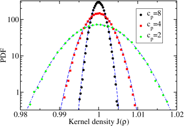
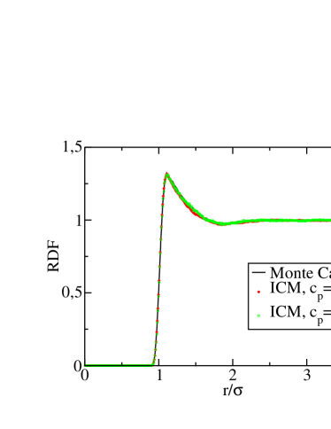
Figure 1: Left, probability density function (PDF) for the average fluid density inside particle kernel, with varying particle compressibilities $\kappa_{p}=1/(\rho_{0}c_{P}^{2})$. Lines corresponds to the normal distribution with the grand canonical ensemble variance in Eq. (43). In all cases the fluid sound velocity is $c_{f}=4$ (parameters are given in table 1). Right, radial distribution of a set of particles at volume fraction $\phi=0.244$ interacting through a repulsive (truncated and shifted) Lennard-Jones potential with strength $\epsilon=k_{B}T$ with mass $m_{e}=0$. Comparison is made between Monte-Carlo simulations and the hydrodynamic code with two different particle compressibilities.

V Acoustic Forces

A central application of the present work is the simuation of acoustophoresis of small particles $(a>0.1\mu\mathrm{m})$ suspended in a fluid subject to MHz ultrasound waves. Such process which is receiving renewed attention in the context of many applications, such as control and manipulation of particles microfluidic devices. We now briefly explain its essential features and the reader is refereed to Refs. Gorkov (1962); Landau and Lifshitz (1987); Doinikov (1997); Settnes and Bruus (2012) for a more comprehensive theoretical description.

We start by considering a fluid under otherwise quiescent condition, which is submitted to an oscillatory mechanical perturbation (maybe through one of its boundaries) which creates a standing acoustic wave. The amplitude of the sound wave is assumed very small, so a standard approach Landau and Lifshitz (1987); Settnes and Bruus (2012) consists on expanding the hydrodynamic fields whose amplitude decrease as increasing powers of the wave amplitude. To second order,

$$\rho = \rho_{0}+\rho_{1}+\rho_{2}$$ (44)

$${\boldsymbol{v}} = {\boldsymbol{v}}_{1}+{\boldsymbol{v}}_{2}.$$ (45)

The time dependence of any hydrodynamic perturbative field (say $\Phi_{i}$ with $i>0$) should have a fast oscillatory contribution with the same frequency as the forced sound wave, i.e. $\Phi_{i}({\boldsymbol{r}},t)=\phi({\boldsymbol{r}})\exp(i\omega t)$. The average $\langle\Phi\rangle=(1/\tau)\int_{0}^{\tau}\Phi(\tau)d\tau$ over the wave period $\tau=2\pi/\omega$ vanishes. Inserting this expansion into the mass and momentum fluid equations leads to a hierarchy of equations at each order in the wave amplitude. At first order the set equations are linear so the time-average of the first-order momentum change rate yields no resulting mean force. However, at second order, the average of non-linear terms (such as $\langle\rho_{0}{\boldsymbol{v}}_{1}{\boldsymbol{v}}_{1}\rangle$) do not vanish ($\langle\cos(\omega t)^{2}\rangle=1/2$) and create the so called radiation force. The leading terms creating the radiation force are already present in an inviscid fluid and for most applications viscous terms only lead to relatively small corrections Settnes and Bruus (2012). Viscous forces are only important near the particle surface $r=a$, where the oscillating fluid velocity field is enforced to match the particle velocity. At a distance $\delta=\sqrt{2\nu/\omega}$ from the particle surface, called viscous penetration length or sonic boundary layer, the fluid inertia (transient term) $\rho\partial_{t}{\boldsymbol{v}}\sim\rho\omega v$ becomes of the same order than viscous forces $\eta\nabla^{2}{\boldsymbol{v}}\sim\eta\delta^{-2}v$. For $|r-a|>\delta$ the fluid can be treated as ideal (inviscid) so the ratio $\delta/a$ determines the relevance of viscous regime Settnes and Bruus (2012). For large values $\delta/a\simeq 5$ the acoustic force reach a plateau which corresponds to the transient (frictional) Stokes force Settnes and Bruus (2012). Here we focus on the inviscid regime ($\delta<<h$) where we expect the inertial (instantaneous and energy conserving) coupling will quantitatively capture the acoustophoretic forces Balboa Usabiaga et al. (2013) on small particles with arbitrary acoustic contrast.

The force exerted by a standing wave on a spherical particle was derived by Gor’kov for the case of an inviscid fluid Gorkov (1962) and recently extended to viscous fluids by Settnes and Bruus Settnes and Bruus (2012). The primary acoustic force can be written in the form

$${\boldsymbol{F}}_{1}=-\boldsymbol{\nabla}U_{ac}$$ (46)

where the acoustic potential $U_{ac}$ is given in Eq. (1). For a sinusoidal wave along the $z$ axis with wavenumber $k$ the expression for the force can be simplified to,

$${\boldsymbol{F}}_{1}=\frac{c_{f}^{2}\Delta\rho^{2}\mathbb{V}k}{4\rho_{0}}\left(f_{1}+\frac{3}{2}f_{2}\right)\sin(2kz),$$ (47)

In the inviscid fluid limit, the viscous layer $\delta=\sqrt{2\nu/\omega}$ is small compared with the wave length $\lambda$ and the particles radius, the coefficients $f_{1}$ and $f_{2}$ are Gorkov (1962); Settnes and Bruus (2012),

$$f_{1} = 1-\frac{\kappa_{p}}{\kappa_{f}}=-\frac{\kappa_{e}}{\kappa_{f}}$$ (48)

$$f_{2} = \frac{2(\rho_{p}-\rho_{0})}{2\rho_{p}+\rho_{0}}=\frac{2m_{e}}{2m_{e}+3\rho_{0}\mathbb{V}}$$ (49)

where the particle density is $\rho_{p}=m_{p}/\mathbb{V}=m_{e}/\mathbb{V}+\rho_{0}$.

In this work we extend the blob model to model a particle with finite compressibility $\kappa_{p}$. Under the local pressure variations of an incoming sound wave a compressible particle pulsates and in doing so it eject fluid mass in the form of a spherical scattered wave. If the particle and fluid compressibilities do not match, the scattered fluid mass is ejected at a rate which differs from the flux of the incoming wave. This difference creates variations in the Archimedes force which is expressed as a (monopolar) radiation force Crum (1974); Settnes and Bruus (2012). The mass of fluid in the kernel is $m_{f}=\mathbb{V}\boldsymbol{J}\rho$ so the mass ejected by pulsation of the particle volume, can be equivalently expressed in terms of changes in the local fluid density. Consider an incoming pressure wave $p_{in}$ which is scattered by the particle. The incoming density wave satisfies $\rho_{in}=\rho_{0}\kappa_{f}p_{in}$, so if the particle were absent, the mass of fluid in the kernel would be $\mathbb{V}\boldsymbol{J}\rho_{in}=\mathbb{V}\rho_{0}\kappa_{f}\boldsymbol{J}p_{in}$. However, the particle modifies the local density according to Eq. (25) and the total mass inside the kernel is then $\mathbb{V}\boldsymbol{J}\rho=\boldsymbol{J}({\boldsymbol{\kappa}}p_{in})\mathbb{V}$ with,

$$\boldsymbol{J}\rho=\left(1+\frac{\kappa_{e}}{\kappa_{f}}\right)\boldsymbol{J}\rho_{in}.$$ (50)

The scattered mass

$$m_{sc}=\mathbb{V}\frac{\kappa_{e}}{\kappa_{f}}\boldsymbol{J}\rho_{in}$$ (51)

is then ejected at a rate,

$$\dot{m}_{sc}=\mathbb{V}\frac{\kappa_{e}}{\kappa_{f}}\frac{d}{dt}\boldsymbol{J}\rho_{in}=\mathbb{V}\frac{\kappa_{e}}{\kappa_{f}}\left[\boldsymbol{J}(\partial_{t}\rho_{in})+\boldsymbol{J}(\nabla\cdot\rho_{in}{\boldsymbol{u}})\right],$$ (52)

where the prefactor $f_{1}=-\kappa_{e}/\kappa_{f}=1-\kappa_{p}/\kappa_{f}$ is in agreement with Gor’kov theoretical result Gorkov (1962); Settnes and Bruus (2012). It is noted that the advective term $\boldsymbol{J}(\nabla\cdot\rho_{in}{\boldsymbol{u}})$ is a second order quantity neglected in theoretical analyses Settnes and Bruus (2012) for low Reynolds numbers, however particle-advective terms need to be included in studies of larger bubbles at non-vanishing Reynolds Pelekasi et al. (2004); Garbin et al. (2009).

VI Acoustic forces: simulations

To create a standing wave in a periodic box we employ a simple method that resembles the experimental setups Haake and Dual (2005). We include a periodic pressure perturbation in all the cells at the plane with coordinate $z=z_{0}$. The pressure perturbation has the form,

$$p^{ext}(t)=\Delta p_{0}\sin(ck_{0}t)h\delta(z-z_{0})$$ (53)

where $k_{0}=2\pi/L$ is the smallest wave number that fits into the simulation box of length $L$. In the discrete setting the delta function should be understood as a Kronecker delta $h\delta(z-z_{0})=\delta^{K}_{zz_{0}}$ so only the cells at the plane $z=z_{0}$ are forced.

A solution for the density modes can be analytically obtained by inserting the forcing pressure (53) into the linearized Navier-Stokes equations and transforming the problem into the Fourier space. This leads to,

$$\rho_{k}=\Delta\rho_{k}\sin(ck_{0}t+\phi)=\frac{k^{2}\Delta p_{0}}{\sqrt{4\Gamma^{2}k^{4}(ck_{0})^{2}+((ck)^{2}-(ck_{0})^{2})^{2}}}\sin(ck_{0}t+\phi).$$ (54)

Where $\Gamma=\nu_{L}/2$ is the sound absorption coefficient (which, in absence of heat diffusion, equals half of the longitudinal viscosity). The singular pressure perturbation $\delta(z-z_{0})$ excites all the spatial modes of the box. However, since $c\gg\Gamma k$, the resonant mode $k=k_{0}$ is by far the dominant one and it is safe to assume that the incoming wave is just a standing wave with wavenumber $k_{0}$,

$$\rho_{in}(z,t)=\Delta\rho_{k=k_{0}}\cos(k_{0}z)\sin(ck_{0}t+\phi)$$ (55)

The validity of this approximation requires working in the linear regime $\Delta\rho_{0}\ll\rho_{0}$ (i.e. low Mach number) which is also satisfied in experiments.

We checked the validity of the present model against the theoretical expression for the (primary) radiation force in Eq. (47), by measuring the acoustic force felt by particles with different mass $m_{e}\neq 0$ or compressibility $\kappa_{e}\neq 0$ than the carrier fluid. To measure the acoustic force at a given location, particles were bounded to an harmonic potential $U_{\mathrm{spring}}=-(1/2)k_{\mathrm{spring}}\left(z-z_{eq}\right)^{2}$ with a given spring constant and equilibrium position $z_{eq}$. The acoustic force displaces the equilibrium position of the spring to an amount $\Delta l$ and its average gives the local acoustic force $F(\hat{z})=k_{\mathrm{spring}}\langle\Delta l\rangle$ where $\hat{z}=z_{eq}+\langle\Delta l\rangle$. In order to conserve the total linear momentum of the system, we place two particles at equal but opposite distances from the pressure perturbation plane $z=z_{0}$ (a wave antinode). In this way the momentum introduced by each harmonic force cancels exactly. Moreover to minimize the effect of secondary forces, particles were placed at different positions in the $x,y$ plane. In most simulations the particles positions were at ${\bf r}_{1}=(1/2,1/2,3/8)L$ and ${\bf r}_{2}=(0,0,-3/8)L$.

VI.1 Monopolar acoustic forces

According to the acoustic potential in Eq. (1), neutrally buoyant particles ($m_{e}=0$) can only feel monopole acoustic forces proportional to the deficiency in particle compressibility $-\kappa_{e}$ with respect to the carrier fluid. [see $f_{1}$ in Eq. (48)]. The left panel of figure 2 represents the acoustic force observed in numerical simulations at different positions in the plane of the standing wave $z$. The particle speed of sound is $c_{p}=2c_{f}$, which corresponds to a particle less compressible than the fluid [$\kappa_{e}=-(3/4)\kappa_{f}$, see Eq. (23)]. Simulations of Fig. 2 were performed in a cubic periodic box of size $L=32\,h$ (see Table I for the rest of simulation parameters). Numerical results exactly recover the dependence of the radiation force with $z$ given by the theoretical expression of the primary radiation force in Eq. (47). However, the force amplitude presents deviations of up to about 10 percent. These deviations tend to zero as the box size is increased, indicating the presence of hydrodynamic finite size effects which, as explained in Sec. VI.3, scale like secondary acoustic forces between particles Crum (1974).

The right panel of figure 2 shows the maximum value of the acoustic force for different particle compressibilities (here, in terms of the ratio $c_{p}/c_{f}=(\kappa_{f}/\kappa_{p})^{1/2}$). It is noted that while the dipole scattering coefficient is bounded $f_{2}\in(-2,1)$, the monopole scattering coefficient is not $f_{1}\in(-\infty,1)$: for incompressible particles it goes to $f_{1}=1$ but diverges if particles are infinitely compressible $c_{p}/c_{f}\rightarrow 0$. This explains why ultrasound is an outstanding tool to manipulate bubbles Garbin et al. (2009). As shown in Fig. 2, the present method correctly describes the divergence of the acoustic force in the limit of large particle compressibility, $\kappa_{p}\rightarrow\infty$.

VI.2 Dipolar acoustic forces

In the left panel of figure 3 we plot the acoustic force along the coordinate $z$ felt by a particle with excess of mass $m_{e}=m_{f}$ and equal compressibility than the fluid $\kappa_{e}=0$. A perfect agreement is found between the numerical results and Eq. 47. In the right panel of the same figure we show the dependence of the maximum acoustic force with the particle-fluid density ratio $\rho_{p}/\rho_{0}$. Again, a quasi-perfect agreement ($1.5\%$ deviation) is observed when compared with the theoretical expression for primary radiation force 47.

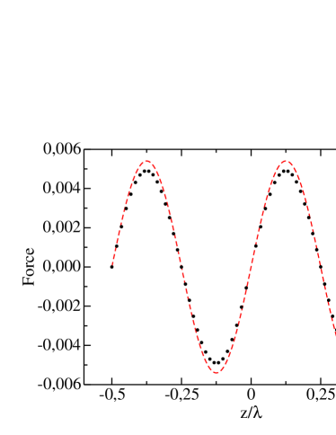
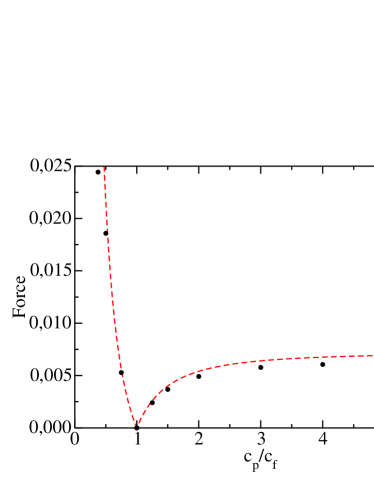
Figure 2: Left panel, acoustic force along the pressure wave for a neutrally-buoyant particle with $c_{p}=2c_{f}$. Right panel, maximum acoustic force versus the ratio $c_{p}/c_{f}$. All the simulation parameters are given in table 1.

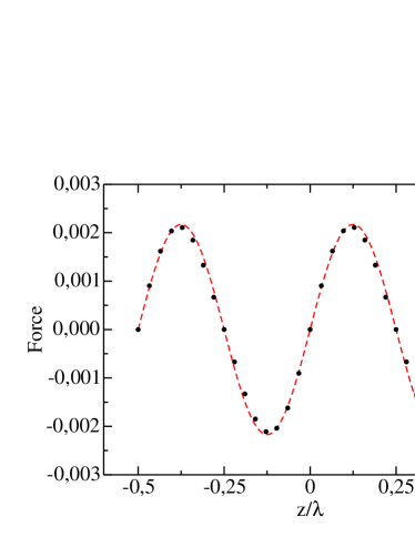
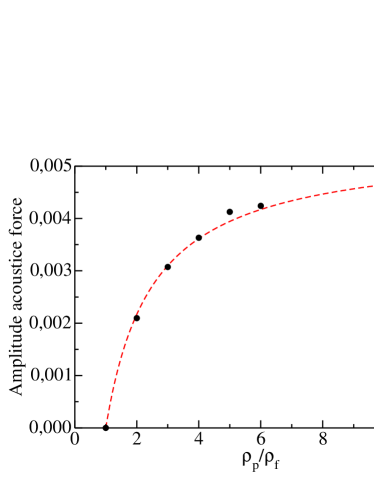
Figure 3: Left panel, acoustic force along the pressure wave for a non-neutrally buoyant particle with speed of sound $c_{p}=c_{f}$. Right, maximum acoustic force versus the particle fluid density ratio $\rho_{p}/\rho_{0}$ for $c_{p}=c_{f}$. Points represent the numerical results and red lines the theoretical prediction. All the simulation parameters are given in table 1.

VI.3 Finite size effects: secondary radiation forces

To understand the discrepancies observed between numerical and theoretical expressions for the primary radiation force, we performed simulations with different box sizes $L$. Results, in Fig. 4, show that discrepancies between the numerical and theoretical forces vanishes as $L$ increases and indicate that these deviations are not algorithmic or discretization errors but rather finite size effects of hydrodynamic origin. Notably, in a periodic box, particles can interact via secondary radiation forces Crum (1974) arising from the scattered waves, irradiated by each particle pulsation Garbin et al. (2009). We now analyze the observed deviations to show that they have the signature of secondary radiation forces.

Secondary radiation forces, also called Bjerknes secondary forces, depend on the particles’ spatial configuration. The problem of elucidating the secondary forces from-and-to an array of scatters is certainly a difficult one Feuillade (1995), but approximate expressions have been proposed for a couple of interacting particles at distance $d$, under certain conditions. In particular, for $R\ll d\ll\lambda$, Crum Crum (1974), Gröschl Gröschl (1998) and others derived the following analytical expression for the secondary forces for two particles at distance $d$ forming at angle $\theta$ with the incident wave is

$${\boldsymbol{F}}_{2}^{(p)} = -\frac{9}{4\pi}\mathbb{V}^{2}\langle p^{2}_{in}(z)\rangle\left[\frac{\omega^{2}\rho_{0}\kappa_{e}^{2}}{9d^{2}}\right]{\bf e_{r}}$$ (56)

$${\boldsymbol{F}}_{2}^{(v)} = \frac{3}{4\pi}\frac{m_{e}^{2}}{2\rho_{0}d^{4}}\langle v^{2}_{in}(z)\rangle\left[(3\cos^{2}\theta-1){\bf e_{r}}+\sin(2\theta){\bf e_{\theta}}\right]$$ (57)

In general, however, the secondary forces depend on the phase difference between the field scattered from particle $1$ (at the particle $2$ location) and the vibration of particle $2$ Crum (1974); Mettin et al. (1997). This phase relation is neglected in the derivation of Eqs. 56, 57, which assumes that $p_{in}(z+d)=p_{in}(z)$ (same for the velocity field) and that both particle oscillates in phase. Details of Bjerknes secondary forces are still under researchGarbin et al. (2009); Pelekasi et al. (2004), for instance, in the case of bubbles, this phase difference might even lead to secondary force reversal (it is attractive for zero phase difference, see Eq. 56).

Let us first analyze secondary forces resulting from an imbalance in the particle density with respect the fluid density, $m_{e}\neq 0$ when particles have similar compressibility as the fluid $\kappa_{e}=0$. In this case, the scattered field has the form of a dipole and decays with the square of the distance Settnes and Bruus (2012). Therefore, secondary forces (dipole-dipole interaction) should decay as the fourth power of the distance, as expressed in Eq. (57). These type of secondary forces are thus short-ranged (and small in magnitude) so they do not induce finite size effects. Consistently, we do not observe any trace of finite size effects in simulations on dipolar acoustic forces, as shown in Fig. 3.

By contrast, particles with some excess in compressibility $\kappa_{e}\neq 0$ vibrate in response to the primary wave, acting as point-sources (monopoles) of fluid mass and creating scattered density waves. These monopolar scattered fields decays like $1/r$ so the secondary interaction between two particles decays with the square of their distance (see Eq. 56). This means that secondary compressibility forces are long ranged and reach image particles beyond the primary box of the periodic cell. Although the exact form of the multiple scattering problem leading to finite size effects in periodic boxes is not easy to solve, it is possible to elucidate some of their essential features. In our setup, due to symmetry, secondary forces are directed in $z$ direction (as the primary one) so the total radiation force on one particle (say $i=1$) should be (summing up to pair reflections in the scattering problem), $F=F_{1}(z_{i})+\sum_{j\neq i}F_{2}(r_{ij})$, with $j$ running over all particles (including periodic images) and $F_{1}$ given by Eq. 47).

For any particle pair, the magnitude of $F_{2}$ is proportional to the product of the fluid mass ejected by each particle, i.e. to $\kappa_{e}^{2}$ (see Eq. 56). Thus, for a given external wave amplitude $\Delta\rho$, the difference between the force $F$ from simulations and the theoretical primary force $F_{1}$ should be proportional to,

$$\Delta F\equiv F-F_{1}\propto\left(\frac{\mathbb{V}\omega}{c_{f}}\right)^{2}\left(\frac{\kappa_{e}}{\kappa_{f}}\right)^{2}$$ (58)

We have measured $\Delta F$ for several compressibilities ratios $|\kappa_{e}/\kappa_{f}|$ and frequencies $\omega$. The left side panel of figure 4 shows $\Delta F$ against $|\kappa_{e}/\kappa_{f}|=|f_{1}|$ for a set of force measures with only differ in the value of $\kappa_{e}$. As predicted by the scaling of secondary forces (58), we get a quadratic dependence $\Delta F\propto|\kappa_{e}/\kappa_{f}|^{2}$. A slight deviation from this trend is observed for the smallest value of $|\kappa_{e}|$ considered (see Fig. 4). Near $\kappa_{e}=0$ both forces (primary $F_{1}$ and secondary force) tend to zero (see Fig. 2) and the evaluation of $\Delta F$ becomes more prone to numerical errors. Values of $\Delta F$ for $\kappa_{e}>0$ (more compressible particles) and $\kappa_{e}<0$ (less compressible) were found to differ in a factor 2; the reason might come from some change in the phase difference of the interacting particles taking place at $f_{1}=0$.

In the right panel of figure 4 we show the relative difference $\Delta F/F_{1}$ obtained in simulations at different forcing frequencies $\omega$. The primary force scales linearly with $\omega$ (see Eq. 47) so, according to Eq. 58, the relative difference $\Delta F/F_{1}$ should also scale linearly in frequency, as observed in Fig. 4 (left). Although an analysis of the total effect of multiple scatterings of secondary forces (Edwald summation) is beyond this work, the inset of this figure shows that the effect of scattered waves from periodic images decreases with the system size.

To further check the resolution of secondary acoustic forces we performed some tests with two neutrally buoyant particles and compressibilities $\kappa_{p}=\kappa_{f}/2$. Particles were located at ${\bf r}_{1}=(0,0,z_{0})$ and ${\bf r}_{2}=(d,0,z_{0})$, where $z_{0}$ is the plane of the pressure antinode where the primary force vanishes. As predicted by the theory (see Eq. 56) the radial secondary forces were found to be attractive. At close distances $d=[2-3]\,h$, we found them to be in very good agreement with Eq. (56) although, at larger distances we found that they decay significantly slower than $d^{-2}$, probably due to the effect of secondary forces coming from the periodic images. In any case, for most practical colloidal applications the effect of secondary forces is small and quite localized. It tends to agglutinate close by colloids to form small clusters, but only after the main primary force collects them in the node-plane of the sound wave. Simulations showed that this local effect of the secondary forces is captured by the present method.

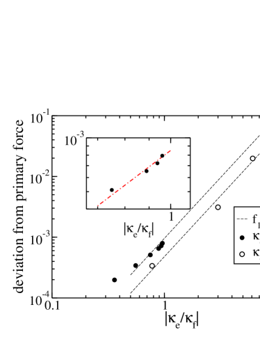
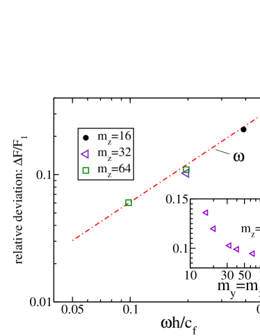
Figure 4: Left panel, deviation of the numerical force from the theoretical primary radiation force $\Delta F=F-F_{1}$ versus the ratio $\kappa_{e}/\kappa_{f}$ with $\kappa_{e}=\kappa_{p}-\kappa_{f}$. All parameters as in figure 2. Right panel, relative deviation $\Delta F/F_{1}$ versus the wave frequency $\omega$. Main figure: simulations in cubic periodic boxes with $m_{z}$ cells per side; inset figure: rectangular boxes with $m_{z}=32$ and varying $m_{x}=m_{y}$ showing that the effect of the periodic images decreases with the system size.

VI.4 Boltzmann distribution and standing waves

Most of the experimental works on acoustophoresis employ particles with diameters above one micrometer or at least close to that size. The reason is that the acoustic force decays strongly with the particles radius and below diameters of one micrometer other forces become equally important in the nano-particle dynamics. As stated previously, one of these forces is the streaming force Nyborg (1965), whose nature and structure is more difficult to control Bruus et al. (2011). Advances in miniaturized devices and in experimental techniques makes easy to guess that acoustophoresis will be soon extended to smaller scales (see the recent work Johansson et al. (2012)). An intrinsic limitation for this miniaturization process comes however from thermal fluctuations which strongly affect the dynamics of nanoscopic particles. Here we study how thermal fluctuations disperse sonicated particles around the minimum of the acoustic potential energy.

A standing waves exert a first-order force that oscillate with the same frequency $\omega$ than the primary wave and averages to zero Bedeaux and Mazur (1974). Since the diffusion of the particles is much slower than the wave period, the first-order force should not have any effect in the slow (time-averaged) dynamics of the particle, which is driven by the second-order radiation force. If the particle mass is not very large (typical particles-fluid density ratio $m_{p}/m_{f}\sim O(1)$) the particle inertia, acting in times of $m_{p}/\xi=(2/9)(m_{p}/m_{f})a^{2}/\nu$, is also negligible in the time scale of Brownian (diffusive) motion ($a^{2}/D$). This indeed is only true provided a large value of the Schmidt number $Sc=\nu/D\sim\nu^{2}\rho a/k_{B}T>>1$ such as those found in solid colloid - liquid dispersion (here $D=k_{B}T/(6\pi\rho\nu a)$ is the Stokes-Einstein diffusion coefficient). Thus, in the Brownian time scale, the relevant forces are the radiation force $F_{1}$, resulting from the acoustic potential Eq. (1), the Stokes friction (which, assuming $\langle{\bf v}\rangle=0$, is equal to $6\pi\eta a{\bf u}$) and dispersion forces from fluid momentum fluctuations. Assuming there are no other momentum sources, such as secondary forces from other particles, and that there is no temperature rising from conversion of acoustic energy into heat, the resulting time-averaged motion can be described by the Brownian dynamics of a particle in an external field, given by the acoustic potential (1). The resulting particle spatial distribution should then follow the Gibbs-Boltzmann distribution,

$$P({\boldsymbol{r}})\propto e^{-U_{ac}({\boldsymbol{r}})/k_{B}T}$$ (59)

This rationale was proposed in an early work by Higashitany et al. Higashitani et al. (1981), who found a good agreement with experiments in very dilute colloidal suspensions. For validation purposes, the simulations presented hereby are done within the range of validity of these approximations. Figure 5 shows the probability density function of the position of a single particle in a standing wave, where different wave amplitudes have been chosen so as to vary the depth of the acoustic potential well 1. The agreement between the numerical result and the Gibbs-Boltzmann distribution is remarkably good and illustrates the difficulty in collecting particles as soon as dispersion forces dominate, $U<k_{B}T$. The present method offers the possibility to investigate what happens if any of the above approximations fail; notably, in situations where non-linear couplings might become relevant, such as the effect of colloidal aggregation, secondary forces between particles or advection by thermal velocity fluctuations Donev et al. (2011).

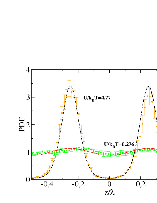
Figure 5: PDF for particles inside an acoustic field. Lines Boltzmann distribution. Circles PDF for a single particle (volume concentration $2.4\cdot 10^{-4}$). Temperature $k_{B}T=1$, the rest of the parameters are given in table 1.

Figure	1	3	2	5
grid spacing $h$	$10$	$10$	$10$	$10$
number of cells	$32^{3}$	$32^{3}$	$32^{3}$	$32^{3}$
fluid density	$1$	$1$	$1$	$1$
shear viscosity $\eta$	$0.5$	$0.5$	$0.5$	$0.5$
bulk viscosity $\zeta$	$0.5$	$1$	$0.5$	$0.5$
fluid speed of sound $c_{f}$	$4$	$4$	$4$	$4$
wave frequency $\omega$	-	$0.0784137$	$0.0784134$	$0.0784134$
pressure forcing $\Delta p$	-	$0.005$	$0.005$	$0.005$ - $0.025$
density perturbation $\Delta\rho$	-	$0.00240249$	$0.00339202$	$0.00339202$ - $0.0140955$
hydrodynamic radius $R_{H}$	$9.9$	$9.9$	$9.9$	$9.9$
particle’s excess of mass $m_{e}$	$0$	$8000$	$0$	$0$
particle’s speed of sound $c_{p}$	$2$-$40$	$4$	$8$	$8$

Table 1: Variables and parameters of the particle (arbitrary units). The forcing frequency is $\omega=2\pi c_{f}/L$ with $L=m_{z}h$ the box size.

VII Concluding remarks

This work presents a coarse-grained model to simulate acoustophoretic phenomena on small particles $O(\mu\mathrm{m})$. The model is based on an Eulerian-Lagrangian approach where the (isothermal) fluctuating hydrodynamics equations are solved in a staggered grid (finite volume scheme) and the colloidal particles move freely in space. The communication between the Eulerian lattice and the particle Lagrangian dynamics is based on the Immersed Boundary (IB) method however, here each particle is described with a single IB kernel. The kernel is used to i) average local fluid properties (e.g. velocity, density) and ii) to convert particle forces into a localized force density field, which acts as a source of fluid momentum. In this way, the particle-fluid interaction conserves local momentum exactly. We use a kinematic coupling between the fluid and the particle which enforces that the kernel-average fluid velocity ($\boldsymbol{J}{\boldsymbol{v}}$) equals the particle velocity, $\boldsymbol{J}{\boldsymbol{v}}={\boldsymbol{u}}$ . The essential property of this type of coupling is that it instantaneously transfers momentum between the particle and the fluid, thus resolving the inertia of both particle and fluid Muser et al. (2013). This instantaneous inertial coupling, as we called it Balboa Usabiaga et al. (2013), is required to resolve ultrasound forces which builds up in sonic times $a/c$, several orders of magnitude faster than friction $a^{2}/\nu$.

The second novelty of the present method is the use of a minimal-resolution model for the particles. We work with the 3-point kernel introduced by Roma and Peskin Roma et al. (1999) which only demand 27 fluid cells per particle. Despite its computational efficiency and simplicity the kernel is physically robust in the sense that it embeds all the essential particle properties (size, mass and, as proved hereby, compressibility). Notably, radiation forces on particles are proportional to their volume, which in the present model is a constant (position-independent) quantity $\mathbb{V}=8h^{3}$ pertaining to the kernel shape and mesh size $h$. In this work the kernel is also used to implement an arbitrary particle compressibility by embedding a small domain with a different equation of state 21. Alternatively, the particle compressibility can be justified from a free energy functional constructed from the particle-fluid (potential) interaction. Here, such functional would have the form,

$${\cal F}\left[\rho,{\boldsymbol{q}}\right]=\frac{\mathbb{V}\epsilon_{pf}}{2\rho_{0}}\left[\boldsymbol{J}(\rho-\rho_{0})\right]^{2},$$ (60)

providing a local fluid chemical potential arising from the particle presence,

$$\mu=\frac{\delta{\cal F}}{\delta\rho}=\frac{\mathbb{V}\epsilon_{pf}}{\rho_{0}}\boldsymbol{S}(\boldsymbol{q}-{\boldsymbol{r}})\left(\boldsymbol{J}\rho-\rho_{0}\right).$$ (61)

Any variation in this chemical potential would then induce a force density field $\rho\nabla\mu$ in the fluid. A Boussinesq-type approximation, valid at low Mach number $\rho\nabla\mu\simeq\rho_{0}\nabla\mu$ leads to the present model equations. In particular, the fluid momentum equation 29 can be then written in a conservative form $\nabla\rho_{0}\mu=\nabla\boldsymbol{S}\Omega$ (see Eqs. 15 and 32). A rigorous connection between our blob-model (based on a mean field approach) and a first-principle derivation of the coupled fluid-particle equations is beyond the scope of the present work. We believe however that such connection is possible and will provide clues to the interaction free energy functional which ultimately, stems from molecular interactions Español and Delgado-Buscalioni (2013). This would certainly open many other applications (wettability) to the present mean field approach. Here however, our main target problem is to model the fluid mass ejected by the pulsation of a colloid’s volume forced by an ultrasound wave. The main benefit of Eq. (14) is that it translates this difficult “mechanical” constraint at the particle surface in a much more simple “thermodynamic” language: it just becomes a local density change. The excellent agreement between simulations and theory Landau and Lifshitz (1987); Gorkov (1962); Settnes and Bruus (2012) confirms that this “translation” works.

The present approach can be safely used to resolve micron particles under several MHz, using for instance, water as carrier fluid $\nu\simeq 10^{-6}\mathrm{m}^{2}/\mathrm{s}$. It is also suited to sub-micron particles $O(0.1\mu\mathrm{m})$, where the thermal drift Higashitani et al. (1981) becomes significant and one needs to include hydrodynamic fluctuations (here they are treated according to the Landau-Lifshitz formalism). Methods for the acoustophoretic control of sub-micron particles are now appearing and indeed require larger frequencies (up to 40MHz range) Johansson et al. (2012). Another potential problem in controlling submicron particles is the drag created by the streaming velocity (the second-order average velocity field $\langle{\boldsymbol{v}}_{2}\rangle$) which at these scales, becomes comparable to the radiation force Bruus et al. (2011). The streaming field $\langle v_{2}\rangle$ spreads over the acoustic boundary layer of any obstacle (e.g. walls) creating, by continuity, an array of vortices. Streaming can be certainly resolved using the present scheme (see Ref.Balboa Usabiaga et al. (2012a) for a description on how to add boundaries in the fluctuating hydrodynamic solver) although, for validation purposes here we use periodic boxes ($\langle{\boldsymbol{v}}_{2}\rangle=0$) and avoid this effect.

As in any coarse-grained description, the present model introduces some artifacts which has to be taken into account when analyzing simulation results. In particular, acoustic forces are proportional to the particle volume $\mathbb{V}$ which, in principle, could be used to define a particle acoustic radius $R_{a}=(6/\pi)^{1/3}h\approx 1.2407h$. This “acoustic radius” however is not the particle hydrodynamic radius, which for the present surface-less, soft-particle model takes a somewhat smaller value $R_{H}=0.91\,h$ Balboa Usabiaga et al. (2013). The blob hydrodynamic radius is calibrated using the Stokes drag on a sphere with no-slip surface Maxey and Riley (1983) (i.e. $g\pi\eta Rv_{0}$ and we use $g=6$ to calibrate $R=R_{H}$). The slow particle dynamics arises from the balance of the acoustic force and the Stokes drag and in practice, to match experimental particle trajectories one should consider that the blob model has a slightly smaller effective skin friction (i.e., $R=R_{a}$ yields $g=4.4$).

The present model cannot properly resolve viscous effects related to the acoustic boundary layer $\delta=\sqrt{2\nu/\omega}$. The radius $R$ of the present one-kernel-particle model is similar to mesh size $h$, so $\delta\sim R\sim h$ and the flow inside the viscous layer is ill-resolved. We observe a limited sensitivity of the resolved dipolar forces to the size of the acoustic layer. For instance, the primary force in Fig. 3 corresponds to $\delta\simeq 0.28\,R_{a}$ and it is found to be about $2\%$ larger than the inviscid limit result ($\delta\rightarrow 0$), however Settnes and Bruus Settnes and Bruus (2012) predict that viscous effects should increase this force in about $10\%$.

Nevertheless, the present approach offers a route to describe these finer details by adding more computational resources to the particle description (larger object resolution, in the spirit of fluid-structure interaction Peskin (2002)). We believe the save in computational cost would be still large compared with fully-Eulerian (particle remeshing) schemes and would allow to resolve the acoustic boundary layer (around “arbitrary” 3D objects) and provide more accurate descriptions of secondary acoustic forces and multiple scattering interaction in multiparticle flows.

Comparison with theoretical expressions show that the present generalization of the IC method accurate resolves acoustic forces in particles with arbitrary acoustic contrast (any excess in particle compressibility and/or mass). The benefit of this minimally-resolved particle model is that although it has a very low computational cost, it naturally includes the relevant non-linear hydrodynamic interactions between particles: mutual hydrodynamic friction, history forces Garbin et al. (2009) convective effects and secondary forces. Interesting non-trivial effects such as changes in the wave pattern due to multiple scattering Feuillade (1995) or sound absorption by colloids or bubbles Kinsler et al. (2000); Riese and Wegdam (1999) can also be simulated . The code Balboa Usabiaga has been written in CUDA and efficiently runs in Graphical Processor Units (GPU): we have verified that simulations with $O(10^{4})$ particles over the colloidal diffusive scale are feasible in affordable computational times.

Appendix A Numerical implementation

We present in this appendix the time-stepping to solve the equations 28-31. The fluid and hybrid (fluid+particle) package (we call fluam) have been coded in CUDA to run on Graphical Processor Units (GPU) and they can be downloaded under GNU license Balboa Usabiaga . Detailed explanation of the numerical scheme for the fluid solver can be found elsewhere Balboa Usabiaga et al. (2012a, b); Balboa Usabiaga et al. (2013). Here we focus on the fluid-particle interaction and in particular in the pressure contribution made by the particles.

A.1 Spatial discretization

The fluid solver, explained in detail in Ref. Balboa Usabiaga et al. (2012a), employs a staggered grid to solve the Navier-Stokes equations. In this grid the scalar variables (i.e. density) are defined at the cell centers, which are located at ${\boldsymbol{r}}_{\boldsymbol{i}}$. On the other hand, vectors, like velocity or momentum, are defined at the cell faces. For example, the x-component of the velocity is defined at ${\boldsymbol{r}}_{\boldsymbol{i}}+\frac{h}{2}\hat{\boldsymbol{x}}$. This nature of the staggered grid should be taken into account when interpolating or spreading variables. Then, the averaging of the fluid density at the particle position $\boldsymbol{q}$ is given by

$$\boldsymbol{J}\rho=\sum_{\boldsymbol{i}\in\mbox{\tiny{grid}}}h^{3}\theta_{h}(\boldsymbol{q}-{\boldsymbol{r}}_{\boldsymbol{i}})\rho_{\boldsymbol{i}}$$ (62)

while the interpolation of the x-component of the velocity is

$$\boldsymbol{J}v^{x}=\sum_{\boldsymbol{i}\in\mbox{\tiny{grid}}}h^{3}\theta_{h}(\boldsymbol{q}-({\boldsymbol{r}}_{\boldsymbol{i}}+\frac{h}{2}\hat{\boldsymbol{x}}))v^{x}_{\boldsymbol{i}+\frac{h}{2}\hat{\boldsymbol{x}}}$$ (63)

The same precaution should be followed when spreading variables at cell centers (i.e. pressure) or at cell faces (forces like $\boldsymbol{\lambda}$ or $\boldsymbol{F}$).

The kernel is defined as the tensor product of three interpolating functions $\phi(r)$, one for each spatial direction $\alpha$

$$\theta_{h}({\boldsymbol{r}})=h^{-3}\prod_{\alpha}\phi\left(\frac{r_{\alpha}}{h}\right)$$ (64)

Although it is not necessary to factorize the kernel in this form, this choice is easy to implement and it is known to give good results Peskin (2002); Dünweg and Ladd (2009) even if the kernel $\theta_{h}(\boldsymbol{q})$ is no longer isotropic. For the interpolating function $\phi(r)$ we employ the three points kernel of Roma and Peskin Roma et al. (1999)

$$\phi(r)=\left\{\begin{array}[]{l l}\frac{1}{3}\left(1+\sqrt{-3r^{2}+1}\right)&|r|\leq 0.5\\ \frac{1}{6}\left(5-3|r|-\sqrt{-3(1-|r|)^{2}+1}\right)&0.5\leq|r|\leq 1.5\\ 0&1.5<|r|\end{array}\right.$$ (68)

which has a good balance between its properties to hide the grid discretization to the particle dynamics and its computational efficiency (each particle only interacts with $27$ cells in three dimensions)Peskin (2002); Roma et al. (1999); Dünweg and Ladd (2009).

A.2 Temporal discretization

Our temporal discretization is based on previous works for deterministic incompressible flows Griffith and Luo (2012) and it was presented in reference Balboa Usabiaga et al. (2012b). The scheme has the following substeps

1. Update the particle half time step

   $$\boldsymbol{q}^{n+\frac{1}{2}}=\boldsymbol{q}^{n}+\frac{\Delta t}{2}\boldsymbol{J}^{n}{\boldsymbol{v}}^{n}$$ (69)

   Note that the particle is advected by the fluid as it could have been expected from the no-slip condition. In the averaging we employ the particle position at time $t^{n}=n\Delta t$ as indicated by the superscript $n$ on $\boldsymbol{J}$.

2. Calculate the external force acting on the particle at time $t^{n+\frac{1}{2}}=(n+\frac{1}{2})\Delta t$

   $${\boldsymbol{F}}^{n+\frac{1}{2}}={\boldsymbol{F}}(\boldsymbol{q}^{n+\frac{1}{2}},t^{n+\frac{1}{2}})$$ (70)

3. Update the fluid state from time $t^{n}=n\Delta t$ to time $t^{n+1}=(n+1)\Delta t$ to obtain the final density $\rho^{n+1}$ and the unperturbed velocity $\boldsymbol{\tilde{v}}^{n+1}$. During this substep we take into account the effect of the external force ${\boldsymbol{F}}^{n+\frac{1}{2}}$ and the particle contribution to the pressure, but we do not impose the no-slip condition, note the absence of the force $\boldsymbol{\lambda}$ on the equations

   $$\partial_{t}\rho+\boldsymbol{\nabla}\cdot({\boldsymbol{g}}) = 0$$ (71)

   $$\partial_{t}{\boldsymbol{g}}+\boldsymbol{\nabla}\cdot({\boldsymbol{g}}{\boldsymbol{v}}) = -\boldsymbol{\nabla}\pi(\rho,\boldsymbol{q}^{n+\frac{1}{2}})+\boldsymbol{\nabla}\cdot\boldsymbol{\sigma}+\boldsymbol{S}^{n+\frac{1}{2}}{\boldsymbol{F}}^{n+\frac{1}{2}}$$ (72)

   To solve this set of equations we employ a third-order Runge-Kutta scheme as explained shortly. During this substep the particle is fixed $\boldsymbol{q}^{n+\frac{1}{2}}=\mbox{const.}$ and so it is the external force ${\boldsymbol{F}}^{n+\frac{1}{2}}$.

4. Calculate the impulse exchange between fluid and particle during the time step

   $$\Delta{\boldsymbol{g}}=\Delta t(\boldsymbol{\lambda}+{\boldsymbol{F}}^{n+\frac{1}{2}})=\frac{m_{e}m_{f}}{m_{e}+m_{f}}\left(\boldsymbol{J}^{n+\frac{1}{2}}\boldsymbol{\tilde{v}}^{n+1}-{\boldsymbol{u}}^{n}\right)$$ (73)

   Where $m_{f}$ is the fluid mass dragged by the particle $m_{f}=\mathbb{V}\boldsymbol{J}^{n+\frac{1}{2}}\rho^{n+1}$.

5. Update the particle velocity

   $${\boldsymbol{u}}^{n+1}={\boldsymbol{u}}^{n}+\frac{\Delta{\boldsymbol{g}}}{m_{e}}={\boldsymbol{u}}^{n}+\frac{m_{f}}{m_{e}+m_{f}}\left(\boldsymbol{J}^{n+\frac{1}{2}}\boldsymbol{\tilde{v}}^{n+1}-{\boldsymbol{u}}^{n}\right)$$ (74)

6. Update the fluid velocity in a momentum conserving manner

   $${\boldsymbol{v}}^{n+1}=\boldsymbol{\tilde{v}}^{n+1}-\frac{\mathbb{V}}{m_{f}}\boldsymbol{S}^{n+\frac{1}{2}}\Delta{\boldsymbol{g}}=\boldsymbol{\tilde{v}}^{n+1}+\mathbb{V}\boldsymbol{S}^{n+\frac{1}{2}}\left({\boldsymbol{u}}^{n+1}-\boldsymbol{J}^{n+\frac{1}{2}}\boldsymbol{\tilde{v}}^{n+1}\right)$$ (75)

   Note that a neutrally-buoyant particle ($m_{e}=0$) is simply advected by the fluid ${\boldsymbol{u}}^{n+1}=\boldsymbol{J}^{n+\frac{1}{2}}\boldsymbol{\tilde{v}}^{n+1}$, as it usually assumed in the IB method Peskin (2002). At the end of this substep the no-slip condition is satisfied in the form ${\boldsymbol{u}}^{n+1}=\boldsymbol{J}^{n+\frac{1}{2}}{\boldsymbol{v}}^{n+1}$ for either neutrally or non-neutrally buoyant particles.

7. Conclude the time step by updating the particle position to time $t^{n+1}=(n+1)\Delta t$

   $$\boldsymbol{q}^{n+1}=\boldsymbol{q}^{n}+\frac{\Delta t}{2}\boldsymbol{J}^{n+\frac{1}{2}}\left({\boldsymbol{v}}^{n+1}+{\boldsymbol{v}}^{n}\right)$$ (76)

The scheme is second order for $m_{e}=0$ (provided that in the third substep the fluid state is updated to at least second order accuracy). However, for $m_{e}\neq 0$ the scheme is only first order although it shows a good accuracy.

In principle, any compressible solver can be used in the substep $3$, we employ the strong stability preserving, third-order accuracy, explicit Runge-Kutta scheme Balboa Usabiaga et al. (2012a); Donev et al. (2010) The scheme is based on a conservative discretization of the Navier-Stokes equation of the form

$$\partial_{t}\boldsymbol{U}=-\boldsymbol{\nabla}\cdot\boldsymbol{F}(\boldsymbol{U},\boldsymbol{q},\boldsymbol{W},t)$$ (77)

where $\boldsymbol{U}=(\rho,{\boldsymbol{g}})$ is an array that collects the fluid variables density and momentum and $\boldsymbol{F}(\boldsymbol{U,\boldsymbol{q},\boldsymbol{W},t})$ represent the flux of the fluctuating Navier-Stokes equations. The flux depends on the particle position through the pressure field $\pi(\rho,\boldsymbol{q})$ and also on the random numbers $\boldsymbol{W}$ through the stochastic fluxes. The Runge-Kutta scheme consist on three substeps where it calculates predictions at times $t^{n+1}=(n+1)\Delta t$, $t^{n+\frac{1}{2}}=(n+\frac{1}{2})\Delta t$ and the final prediction at time $t^{n+1}=(n+1)\Delta t$. In each substep the following increment is calculated

$$\Delta\boldsymbol{U}(\boldsymbol{U},\boldsymbol{q},\boldsymbol{W},t)=-\Delta t\boldsymbol{\nabla}\cdot{\boldsymbol{F}}(\boldsymbol{U},\boldsymbol{q},\boldsymbol{W},t)$$ (78)

and the Runge-Kutta substep are

$$\widetilde{\boldsymbol{U}}^{n+1} = \boldsymbol{U}^{n}+\Delta\boldsymbol{U}(\boldsymbol{U}^{n},\boldsymbol{q}^{n+\frac{1}{2}},\boldsymbol{W}^{n}_{1},t^{n})$$ (79)

$$\boldsymbol{U}^{n+1/2} = \frac{3}{4}\boldsymbol{U}^{n}+\frac{1}{4}\left(\widetilde{\boldsymbol{U}}^{n+1}+\Delta\boldsymbol{U}(\widetilde{\boldsymbol{U}}^{n+1},\boldsymbol{q}^{n+\frac{1}{2}},\boldsymbol{W}_{2}^{n},t^{n+1})\right)$$ (80)

$$\boldsymbol{U}^{n+1} = \frac{1}{3}\boldsymbol{U}^{n}+\frac{2}{3}\left(\boldsymbol{U}^{n+1/2}+\Delta\boldsymbol{U}(\boldsymbol{U}^{n+1/2},\boldsymbol{q}^{n+\frac{1}{2}},\boldsymbol{W}_{3}^{n},t^{n+\frac{1}{2}})\right)$$ (81)

The last substep can be written in the well known form

$$\boldsymbol{U}^{n+1}=\boldsymbol{U}^{n}+\frac{1}{6}\left(\Delta\boldsymbol{U}^{n}+4\Delta\boldsymbol{U}^{n+1/2}+\Delta\widetilde{\boldsymbol{U}}^{n+1}\right)$$ (82)

that shows that it is a centered scheme. The combination of random numbers is such that guarantees a third-order weak accuracy in the linear setting Donev et al. (2010); Balboa Usabiaga et al. (2012b); Delong et al. (2013) and they are

$$\boldsymbol{W}_{1}^{n} = \boldsymbol{W}_{A}^{n}-\sqrt{3}\boldsymbol{W}_{B}^{n}$$ (83)

$$\boldsymbol{W}_{2}^{n} = \boldsymbol{W}_{A}^{n}+\sqrt{3}\boldsymbol{W}_{B}^{n}$$ (84)

$$\boldsymbol{W}_{3}^{n} = \boldsymbol{W}_{A}^{n}$$ (85)

$$\langle\boldsymbol{W}_{C}^{n}({\boldsymbol{r}}_{i})\boldsymbol{W}_{D}^{m}({\boldsymbol{r}}_{j})\rangle = \delta_{CD}\delta_{nm}\delta_{ij}$$ (86)

The only difference with previous works is that here the pressure depends on the particle position, which along the Runge-Kutta step is fixed $\boldsymbol{q}^{n+\frac{1}{2}}=\mbox{constant}$. The three pressures used in the fluid update are

$$\pi^{n} = c_{f}^{2}\rho^{n}+\epsilon_{pf}\mathbb{V}\boldsymbol{S}^{n+\frac{1}{2}}\left(\boldsymbol{J}^{n+\frac{1}{2}}\rho^{n}-\rho_{0}\right)$$ (87)

$$\widetilde{\pi}^{n+1} = c_{f}^{2}\widetilde{\rho}^{n+1}+\epsilon_{pf}\mathbb{V}\boldsymbol{S}^{n+\frac{1}{2}}\left(\boldsymbol{J}^{n+\frac{1}{2}}\widetilde{\rho}^{n+1}-\rho_{0}\right)$$ (88)

$$\pi^{n+\frac{1}{2}} = c_{f}^{2}\rho^{n+\frac{1}{2}}+\epsilon_{pf}\mathbb{V}\boldsymbol{S}^{n+\frac{1}{2}}\left(\boldsymbol{J}^{n+\frac{1}{2}}\rho^{n+\frac{1}{2}}-\rho_{0}\right)$$ (89)

A.3 Convergence analysis: comment on the variance of the kernel density

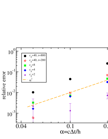
Figure 6: Deviation between the input particle speed of sound $c_{p}=\sqrt{c_{f}^{2}+\epsilon_{pf}}$ and that obtained from the best fit of the kernel density $\boldsymbol{J}\rho$ PDF to the grand-canonical Gaussian distribution of Eq. (43) (see Fig. 1). The abscissa correspond to the CFL number $\alpha=c\Delta t/h$ where the speed of sound $c$ is the maximum value between the fluid and particle speed of sound. In the simulation with cell Reynolds number $r=200$ the viscosities where $\eta=\zeta=2$, the rest of simulation parameters are given in Table I.

We found that the PDF of the interpolated density $\boldsymbol{J}\rho$ follows a Gaussian distribution for all the considered cases. However, its variance presents some numerical deviation if large time steps are used. As we said in section IV this variance can be used to measure the convergence order of our scheme. In figure 6 we present the relative error between the input particle speed of sound $c_{p}=\sqrt{c_{f}^{2}+\epsilon_{pf}}$ and the numerical measure obtained from the variance $\mbox{Var}[(\boldsymbol{J}\rho)^{2}]=\rho_{0}k_{B}T\mathbb{V}^{-1}/c_{p}^{2}$. For neutrally buoyant particles the scheme is second order accurate, as we anticipated. It is interesting to note that when the cell Reynolds number $r=ch/\nu$ is large, the errors are larger for a given speed of sound and time step. The cell Reynolds number measures the relative importance of the advection relative to the viscous terms and it seems that high advective terms reduce the accuracy of the present scheme.

References

- Settnes and Bruus (2012) M. Settnes and H. Bruus, Physical Review E 85, 016327 (2012).
- King (1934) L. V. King, Proceedings of the Royal Society of London A 147, 212 (1934).
- Yosioka and Kawasima (1955) K. Yosioka and Y. Kawasima, Acustica 5, 167 (1955).
- Gorkov (1962) L. P. Gorkov, Sov. Phys. Dokl. 6, 773 (1962).
- Wang and Dual (2011) J. Wang and J. Dual, Journal of Acoustical Society of America 129, 3490 (2011).
- Doinikov (1994) A. A. Doinikov, Proceedings: Mathematical and Physical Sciences 447, 447 (1994).
- Doinikov (1997) A. A. Doinikov, Journal of Acoustical Society of America 101, 713 (1997).
- Dion et al. (1982) J. L. Dion, A. Malutta, and P. Cielo, Journal of the Acoustical Society of America 72, 1524 (1982).
- Friend and Yeo (2011) J. Friend and L. Y. Yeo, Review of Modern Physics 83, 647 (2011).
- Ding et al. (2012) X. Ding, J. Shi, S.-C. S. Lin, S. Yazdi, B. Kiralya, and T. J. Huang, Lab on a Chip 12, 2491 (2012).
- Oberti et al. (2007) S. Oberti, A. Neild, and J. Dual, Journal of Acoustical Society of America 121, 778 (2007).
- Haake et al. (2005) A. Haake, A. Neild, G. Radziwill, and J. Dual, Biotechnology and Bioengineering 92, 8 (2005).
- Higashitani et al. (1981) K. Higashitani, M. Fukushima, and Y. Matsuno, Chemical Engineering Science 36, 1877 (1981).
- Skafte-Pedersen (2008) P. Skafte-Pedersen, Master’s thesis, Technical University of Denmark (2008).
- Dual et al. (2012) J. Dual, P. Hahn, I. Leibacher, D. Möller, T. Schwarz, and J. Wang, Lab on a Chip 12, 4010 (2012).
- Maxey and Riley (1983) M. R. Maxey and J. J. Riley, Physics of Fluids 26, 883 (1983).
- Muller et al. (2012) P. B. Muller, R. Barnkob, M. J. H. Jensenc, and H. Bruus, Lab on a Chip 12, 4617 (2012).
- Feuillade (1996) C. Feuillade, Journal of the Acoustical Society of America 99, 3412 (1996).
- Wang and Dual (2009) J. Wang and J. Dual, Journal of Physics A: Mathematical and Theoretical 42, 285502 (2009).
- Barrios and Rechtman (2008) G. Barrios and R. Rechtman, Journal of Fluid Mechanics 596, 191 (2008).
- Hasegawa (1979) T. Hasegawa, Journal of the Acoustical Society of America 65, 32 (1979).
- Dünweg and Ladd (2009) B. Dünweg and A. J. C. Ladd, Advances in Polymer Science 221, 89 (2009).
- Peskin (2002) C. S. Peskin, Acta Numerica p. 479 (2002).
- Balboa Usabiaga et al. (2012a) F. Balboa Usabiaga, J. B. Bell, R. Delgado-Buscalioni, A. Donev, T. G. Fai, B. E. Griffith, and C. S. Peskin, Multiscale Modeling & Simulation 10, 1369 (2012a).
- Roma et al. (1999) A. M. Roma, C. S. Peskin, and M. J. Berger, J. Comput. Phys. 153, 509 (1999).
- Balboa Usabiaga et al. (2013) F. Balboa Usabiaga, I. Pagonabarraga, and R. Delgado-Buscalioni, Journal of Computational Physics 235, 701 (2013).
- Lomholt and Maxey (2003) S. Lomholt and M. R. Maxey, Journal of Computational Physics 184, 381 (2003).
- Tatsumi and Yamamoto (2012) R. Tatsumi and R. Yamamoto, Physical Review E 85, 066704 (2012).
- Vazquez-Quesada et al. (2012) A. Vazquez-Quesada, M. Ellero, and P. Espanol, Microfluidics and Nanofluidics 13, 249 (2012).
- Balboa Usabiaga et al. (2012b) F. Balboa Usabiaga, R. Delgado-Buscalioni, B. E. Griffith, and A. Donev, Inertial coupling method for particles in an incompressible fluid (2012b), URL http://arxiv.org/abs/1212.6427.
- Atzberger (2011) P. J. Atzberger, Journal of Computational Physics 230, 2821 (2011).
- Kim and Karrila (1991) V. S. Kim and S. J. Karrila, Microhydrodynamics: Principles and Selected Applications (Butterworth-Heinemann Ltd., 1991).
- Español and Delgado-Buscalioni (2013) P. Español and R. Delgado-Buscalioni (2013).
- Yeo and Maxey (2010) K. Yeo and M. R. Maxey, Journal of Computational Physics 229, 2401 (2010).
- Bedeaux and Mazur (1974) D. Bedeaux and P. Mazur, Physica 78, 505 (1974).
- Kinsler et al. (2000) L. E. Kinsler, A. R. Frey, A. B. Coppens, and J. V. Sanders, Fundamental of Acoustics (fourth edition) (John Wiley and Sons, 2000).
- Landau and Lifshitz (1987) L. D. Landau and E. M. Lifshitz, Fluid Mechanics (Pergamon Press, 1987).
- Fabritiis et al. (2007) G. D. Fabritiis, M. Serrano, R. Delgado-Buscalioni, and P. V. Coveney, Physical Review E 75, 026307 (2007).
- Donev et al. (2010) A. Donev, E. Vanden-Eijnden, A. L. García, and J. B. Bell, Communications in Applied Mathematics and Computational Science 5, 149 (2010).
- Giupponi et al. (2007) G. Giupponi, G. D. Fabritiis, and P. V. Coveney, Journal of Chemical Physics 126, 154903 (2007).
- de Groot S. and P. (1984 (reprinted) de Groot S. and M. P., Non equilibrium thermodynamics (Dover, 1984 (reprinted)).
- Bschorr (1999) . Bschorr, J. Acoust. Soc. Am. 106, 3730 (1999).
- Larraza and Denardo (1998) A. Larraza and B. Denardo, Phys. Lett. A 248, 151 (1998).
- Crum (1974) L. A. Crum, J. Acoust. Soc. Am. 57, 1363 (1974).
- Pelekasi et al. (2004) N. Pelekasi, A. Gaki, A. Doinikov, and J. A. Tsamopoulos, J. Fluid Mech. 500, 313 (2004).
- Garbin et al. (2009) V. Garbin, B. Dollet, D. Lohse, M. Versluis, N. de Jong, dLeen van Wijngaarden, A. Prosperetti, M. Overvelde, D. Cojoc, and E. D. Fabrizio, Phys. Fluids 21, 092003 (2009).
- Haake and Dual (2005) A. Haake and J. Dual, Journal of the Acoustical Society of America 117, 2752 (2005).
- Feuillade (1995) C. Feuillade, Journal of the Acoustical Society of America 98, 1178 (1995).
- Gröschl (1998) M. Gröschl, Acustica 84, 432 (1998).
- Mettin et al. (1997) R. Mettin, I. Akhatov, U. Parlitz, C. D. Ohl, and W. Lauterborn, Phys. Rev. E 56, 2924 (1997), URL http://link.aps.org/doi/10.1103/PhysRevE.56.2924.
- Nyborg (1965) W. L. M. Nyborg, Physical Acoustics 2, 265 (1965).
- Bruus et al. (2011) H. Bruus, J. Dual, J. Hawkes, M. Hill, T. Laurell, J. Nilsson, S. Radel, S. Sadhal, and M. Wiklund (Lab on a chip, 2011).
- Johansson et al. (2012) L. Johansson, J. Enlund, S. Johansson, I. Katardjiev, and V. Yantchev, Biomed. Microdevices 14, 279 (2012).
- Donev et al. (2011) A. Donev, J. B. Bell, A. de la Fuente, and A. L. Garcia, Physical Review Letters 106, 204501 (2011).
- Muser et al. (2013) M. H. Muser, G. Sutmann, and R. G. Winkler, eds., Inertial Coupling Method for Blob-Model Particle Hydrodynamics: From Brownian Motion to Inertial Effects, vol. 46 of Hybrid Particle-Continuum Methods in Computational Materials Physics, Publication Series of the John von Neumann Institute for Computing (NIC) (2013).
- Riese and Wegdam (1999) D. O. Riese and G. H. Wegdam, Physical Review Letters 82, 1676 (1999).
- (57) F. Balboa Usabiaga, Fluam, URL https://code.google.com/p/fluam/.
- Griffith and Luo (2012) B. E. Griffith and X. Luo, Hybrid finite difference/finite element version of the immersed boundary method (2012).
- Delong et al. (2013) S. Delong, B. E. Griffith, E. Vanden-Eijnden, and A. Donev, Physical Review E 87, 033302 (2013).