Model of hard spheroplatelets near a hard wall

Abstract

A system of hard spheroplatelets near an impenetrable wall is studied in the low-density Onsager approximation. Spheroplatelets have optimal shape between rods and plates, and the direct transition from the isotropic to biaxial nematic phase is present. A simple local approximation for the one-particle distribution function is used. Analytical results for the surface tension and the entropy contributions are derived. The density and the order-parameter profiles near the wall are calculated. The preferred orientation of the short molecule axes is perpendicular to the wall. Biaxiality close to the wall can appear only if the phase is biaxial in the bulk.

I Introduction

Biaxial nematic phases attracting experimental, theoretical, and computer simulation research since its first prediction by Freiser 1970_Freiser . There phases are characterized by an orientational order along three perpendicular directions and by the existence of three distinct optical axes. They are very interesting from both the fundamental and the technological points of view 2008_Berardi_JP , 2010_Tschierske . Biaxial materials could offer a possibility of fast switching of the second director and better viewing characteristics.

In practical applications liquid crystals are always placed in limited space and even a weak interaction with a limiting surface can change the structure of a liquid crystal near the boundary. A basic model for a phase boundary is the smooth hard planar wall. Despite its simplicity it can induce interesting phenomena.

The behavior of hard biaxial molecule fluids near a hard surface is poorly understood. In this paper we study the nematic-wall and the isotropic-wall interfaces assuming that biaxial molecules interact with one another and with the wall only via hard-core repulsion. Analytical results for the surface tension and the entropy contributions are derived. We find the preferred orientation of the phase composed of the most biaxial spheroplatelets with the optimal shape between rods and plates. For such molecules there is the direct transition from the isotropic phase to the biaxial nematic phase on increasing the density. The preferred phase orientation minimize the nematic-wall surface tension. The density and order-parameter profiles are calculated in the case of the isotropic and the biaxial nematic phase.

The paper is organized as follows. In Sec. II interfacial phenomena and biaxial molecules studies are briefly reviewed in order to provide the background for our studies. In Sec. III the statistical theory of the phase ordering is provided for the case of the hard molecules at the hard wall in the low-density limit. In Sec. IV the theory is applied to the system of hard spheroplatelets where the direct transition from the isotropic phase to the biaxial nematic phase is present in the bulk. Section V contains a summary.

II Background

In order to make the paper self-contained, we collect the relevant definitions and fact concerning interfacial phenomena and biaxial molecule studies.

II.1 Fluid interfacial phenomena

There are many fluid interfacial phenomena, such as anchoring, critical adsorption, pre-wetting and wetting transitions 1991_Jerome . The possible structural rearrangements in the vicinity of the interface are (1) periodic modulations of density, (2) polar ordering of molecular dipoles, and (3) modifications of the scalar order parameter 2003_Kleman_Lavrentovich . Anchoring is a fixing of the phase orientation by the surface with lifting the orientation in the bulk via the elastic forces. In confined geometry, phase transitions are usually shifted with respect to the transitions observed in infinite geometry.

Let us consider the case of a second-order transition from a disordered to an ordered phase. The order parameter fluctuations appear in the bulk with a correlation length which diverges at the transition. The correlation length at the surface becomes infinite in a direction parallel to the surface plane. This creates an ordered layer at the surface in which the order parameter decreases exponentially to zero in the bulk over a penetration length. The penetration length is equal to the correlation length and thus diverges at the transition. This phenomenon is called critical adsorption 1991_Jerome .

When the transition is first order, the situation is more complex. Partial or complete wetting can appear depending on the values of a contact angle. When one explores the coexistence curve between phases, one can go from a partial wetting regime to a complete wetting regime via a wetting transition.

II.2 Studies of hard biaxial molecules

Computer simulations studies of anisotropic hard molecules have confirmed that hard-core interactions are essential for liquid crystal phase behavior 1993_Allen . Over the years a variety of hard-particle models have been studied theoretically and by using computer simulations. These investigations have shown that hard-particle fluids can exhibit many liquid-crystalline phases, such as uniaxial and biaxial nematic 1990_Allen , smectic, crystal, and plastic solid phases 1985_Frenkel_Mulder , 1987_Stroobants .

Several types of biaxial molecule fluids were investigated: ellipsoids with three different axes 1990_Allen , 1997_Camp_Allen , 1997_Vega , 1997_Zakhlevnykh_Sosnin , 2007_McBride_Lomba , biaxial Gay-Berne particles 1995_Berardi , 1998_Berardi , 2000_Berardi_Zannoni , 2001_Zannoni , 2008_Berardi_JCP , rectangular parallelepipeds 2008_John , 2011_Martinez-Raton , spheroplatelets, and spherocuboids 2005_Mulder . Singh and Kumar developed a theory with a general convex-body coordinate system that can be used to describe any hard convex body 1996_Singh_Kumar , 2001_Singh_Kumar . The results can be utilized in the study of structural, thermodynamic, and transport properties of ellipsoidal fluids.

The hard spheroplatelet is a natural generalization of the spherocylinder. In 1986 Mulder expressed the pair-excluded volume at fixed orientation in closed form 1986_Mulder . Later the phase diagram of the hard spheroplatelet fluid was proposed as a result of bifurcation analysis in the low-density Onsager approximation 1989_Mulder . The density versus particle biaxiality phase diagram displays a cusp-shaped biaxial nematic phase intervening between two uniaxial nematic phases. Holyst and Poniewierski studied the Landau bicritical point at which a direct transition from the isotropic phase to the biaxial nematic phase occurs 1990_Holyst_Poniewierski . A dense system of hard biaxial molecules (spheroplatelets and ellipsoids) was considered using a density functional theory. They found that the density of the isotropic phase at the Landau bicritical point was always higher than that at the isotropic-nematic transition in the limit of uniaxial molecules.

In 1991 Taylor extended the pair-excluded volume to the case of non-identical spheroplatelets 1991_Taylor . In the same year Taylor and Herzfeld studied nematic and smectic order in a fluid of hard biaxial spheroplatelets 1991_Taylor_Herzfeld . They used scaled particle theory for the fluid configurational entropy, in conjunction with a cell description of translational order. When the possibility of translational order was considered, the phase diagram displayed three distinct smectic A phases, columnar and crystalline ordering for higher densities (packing greater then 0.6). For low and intermediate densities the diagram was identical with previous findings (the isotropic phase, the two uniaxial nematic phases separated by the biaxial nematic phase). The necessity of further studies of the Landau point region was noted.

In 2009 van der Pol et al. found biaxial nematic and biaxial smectic phases in a colloidal model system of mineral goethite particles with a simple boardlike shape and short-range repulsive interaction 2009_Pol . The biaxial nematic phase was stable over a large concentration range and the uniaxial nematic phase was not found. Other studies showed that shape polidispersity of particles can stabilize the biaxial nematic phase, and it can induce a novel topology in the phase diagram 2003_Vanakaras , 2011_Belli . Another stabilizing factor is a small tetrahedral deformation of particles as was shown within the extended Straley model 2011_Kapanowski .

Recently Peroukidis et al. calculated the full phase diagram of hard biaxial spheroplatelets by means of Monte Carlo simulations 2013_Peroukidis_Vanakaras , 2013_Peroukidis . New classes of phase sequences were identified: $I-[N_{+}]-SmA$, $I-[N_{b-}-N_{b+}]-SmA$ (crossover), $I-[N_{-}]-SmA$, $I-[N_{-}]-Col_{x}$ (columnar phases), $I-Cub$ (cubatic phases). The brackets indicate phases that may be absent. The most interesting finding was the crossover between two distinct biaxial nematic states. The formation of anisotropic supramolecular assemblies was demonstrated.

II.3 Hard molecules at the interface

Properties of liquid crystal phases in the bulk and at the surface generally are not the same. Different physical systems were studied in the past: fluids with uniaxial molecules in contact with a single (hard or attractive) wall, confined by two walls (thin cells) or curved surfaces 2012_Zhang . Let us recall the main results concerning solid-fluid interfaces. We will not discuss nematic free surfaces and thin films.

In 1984 Telo da Gama studied wetting transitions at a solid-fluid interface using attractive walls and the attractive forces with a hard core for molecular interactions 1984_Telo_da_Gama . The wetting transitions were always weakly first order. In 1988 Poniewierski and Holyst studied a system of hard spherocylinders in contact with a single hard wall 1988_Poniewierski_Holyst_PRA . They used a simple local approximation for the one-particle distribution function and showed that the preferred orientation of the nematic director is parallel to the wall. The density and order-parameter profiles were calculated. The nematic main order parameter was enhanced near the wall even though the density was reduced. The wall-induced biaxiality was small in the interfacial region. Wetting by the nematic phase occurred at the nematic-isotropic coexistence. Later the stability of the uniaxial solution close to the wall was investigated in the limit of very long molecules 1993_Poniewierski , and the bifurcation point was found. The nematic-phase–isotropic-phase interface for hard spherocylinders was studied in Ref. 1988_Holyst_Poniewierski_PRA .

A hard-rod fluid confined by two parallel wall was studied by Mao et al. 1997_Mao . The aim of this work was to calculate the depletion force between the plates due to confinement of the rods. Van Roij et al. investigated the phase behavior of colloidal hard-rod fluids ($L/D=15$) near a single wall and confined in a slit pore 2000_Roij , 2000_Roij_JCP , 2001_Dijkstra , 2005_Dijkstra . They obtained (1) a wall-induced surface transition from uniaxial to biaxial symmetry, (2) complete orientational wetting of the wall-isotropic fluid interface by a nematic film, and (3) capillary nematization, with a capillary critical point, induced by confinement in the slit pore.

The properties of a model suspension of hard colloidal platelets with continuous orientations and vanishing thickness were studied using several methods by Reich et al. 2007_Reich . It is interesting that this system is not described well by the Onsager theory, and a scaling argument known from thin rods does not hold. The fundamental measure theory density functional was used, which includes contributions to the free energy that are of the third order in density.

III Theory

The aim of this section is to develop the statistical theory of the phase ordering for the case of the hard molecules at the hard wall in the low-density limit. The expressions for the density, the order parameters, and the surface tension will be derived.

III.1 Description of the system

The system of hard spheroplatelets in the presence of a hard wall is considered. A spheroplatelet can be described as a rectangular block with dimensions $2a\times b\times c$, capped with quarter spheres of radius $a$ and half-cylinders with radius $a$ and lengths $b$ and $c$ such as to produce a piece-wise smooth convex body; see Fig. 1. The position and the orientation of a spheroplatelet are determined by $\vec{r}$ and the three Euler angles $R=(\phi,\theta,\psi)$, respectively. Alternatively, the orientation can be described by the three orthonormal vectors $(\vec{l},\vec{m},\vec{n})$. The $z$ axis is chosen to be perpendicular to the wall. The density of the fluid at $z=+\infty$ is $\rho_{0}$.

Figure 1: Front, side, and top view of a spheroplatelet.

The grand thermodynamical potential $\Omega$ as a functional of the one-particle distribution function $\rho(\vec{r},R)$ has the following form:

$$\beta\Omega\{\rho\}=\beta F_{id}\{\rho\}+\beta F_{ex}\{\rho\}\\ +\beta\int d\vec{r}dR\rho(\vec{r},R)[V_{ext}(\vec{r},R)-\mu],$$ (1)

where the ideal gas contribution is

$$\beta F_{id}\{\rho\}=\int d\vec{r}dR\rho(\vec{r},R)\{\ln[\Lambda\rho(\vec{r},R)]-1\},$$ (2)

$\mu$ is the chemical potential, $\beta=1/k_{B}T$ is the Boltzmann factor, $V_{ext}$ stands for the external potential, and $\Lambda$ is the (irrelevant) thermal volume of molecules. $F_{ex}$ is the excess part of the free energy corresponding to the interactions between molecules. We assume the low-density Onsager approximation for $F_{ex}$, i.e.,

$$\beta F_{ex}=-\frac{1}{2}\int d\vec{r}_{1}dR_{1}d\vec{r}_{2}dR_{2}\rho(\vec{r}_{1},R_{1})\rho(\vec{r}_{2},R_{2})f_{12},$$ (3)

where $f_{12}$ stands for the Mayer function, which is equal to $-1$ when two molecules overlap and $0$ otherwise. The one-particle distribution function has the normalization

$$\int d\vec{r}dR\rho(\vec{r},R)=N.$$ (4)

The expression for the external potential exerted on a molecule by the hard wall reads as follows:

$$V_{ext}(z,R)=\left\{\begin{array}[]{ll}+\infty&\mbox{for}\ z<z_{m}(R),\\ 0&\mbox{for}\ z>z_{m}(R),\end{array}\right.$$ (5)

where $z_{m}(R)=a+(b|m_{z}|+c|n_{z}|)/2$ stands for the minimal distance between the wall and a molecule of orientation $R$. The minimization of $\Omega\{\rho\}$ with respect to $\rho(\vec{r},R)$ leads to the integral equation for $\rho(\vec{r},R)$:

$$\ln[\Lambda\rho(\vec{r}_{1},R_{1})]+\beta V_{ext}(\vec{r}_{1},R_{1})\\ -\int d\vec{r}_{2}dR_{2}\rho(\vec{r}_{2},R_{2})f_{12}=\beta\mu.$$ (6)

In the absence of an external potential Eq. (6) has a spatially uniform solution $\rho(\vec{r}_{1},R_{1})=\rho_{0}f(R)$, where $f(R)$ is the orientational distribution function normalized to unity. For the isotropic phase $f(R)=1/8\pi^{2}$, for the uniaxial nematic phase $f(R)=f(\vec{l}\cdot\vec{N},\vec{n}\cdot\vec{N})$, and for the biaxial nematic phase $f(R)=f(\vec{l}\cdot\vec{L},\vec{l}\cdot\vec{N},\vec{n}\cdot\vec{L},\vec{n}\cdot\vec{N})$. The unit orthogonal vectors $(\vec{L},\vec{M},\vec{N})$ determine three axes of the $D_{2h}$ symmetry of the biaxial nematic phase. In the uniaxial nematic phase with $D_{\infty h}$ symmetry only the $\vec{N}$ vector survives.

III.2 The liquid crystal-wall surface tension

When the wall is present, instead of solving Eq. (6), we approximate $\rho(z,R)$ as follows 1988_Poniewierski_Holyst_PRA :

$$\rho(z,R)=\rho_{0}f(R)\exp[-\beta V_{ext}(z,R)].$$ (7)

Let us note that the density profiles obtained from (7) will not exhibit the short-range oscillatory behavior that is expected close to the wall. It is assumed that the directors $(\vec{L},\vec{M},\vec{N})$ do not change throughout the sample. Substitution of (7) into (1) and subtraction of the bulk term leads to the expression for the liquid crystal-wall surface tension $\gamma$ 1988_Poniewierski_Holyst_PRA ,

$$\beta\gamma=-(S_{rot}+S_{tr,id}+S_{tr,ex})/k_{B}-\beta\Delta\mu\Gamma,$$ (8)

where $S_{rot}$, $S_{tr,id}$, and $S_{tr,ex}$ are the surface entropies per unit area,

$$\beta\Delta\mu=\beta\mu-\ln[\Lambda\rho_{0}/(8\pi^{2})];$$ (9)

$$\begin{split}\Gamma&=\int_{0}^{\infty}dzdR[\rho(z,R)-\rho_{0}f(R)]\\ &=-\rho_{0}\int dRf(R)z_{m}(R)\end{split}$$ (10)

stands for the adsorption 1988_Poniewierski_Holyst_PRA . The rotational entropy $S_{rot}$ comes only from the ideal term in the free energy. According to the usual convention, the rotational entropy is defined in such a way that it vanishes for the isotropic phase

$$S_{rot}/k_{B}=\rho_{0}\int dRf(R)z_{m}(R)\ln[8\pi^{2}f(R)].$$ (11)

The translational entropy have two contributions: $S_{tr,id}$ from the ideal term and $S_{tr,ex}$ from the excess term:

$$S_{tr,id}/k_{B}=-\rho_{0}\int dRf(R)z_{m}(R),$$ (12)

$$S_{tr,ex}/k_{B}=\\ \frac{1}{2}\rho_{0}^{2}\int dR_{1}dR_{2}f(R_{1})f(R_{2})z_{m}(R_{1})K(R_{1},R_{2})\\ +\frac{1}{2}\rho_{0}^{2}\int dR_{1}dR_{2}f(R_{1})f(R_{2})L(R_{1},R_{2}),$$ (13)

where

$$L(R_{1},R_{2})=\int_{z_{m}(R_{1})-z_{m}(R_{2})}^{\infty}dz_{12}\\ \times\left[z_{12}-z_{m}(R_{1})+z_{m}(R_{2})\right]V(|z_{12}|,R_{1},R_{2}),$$ (14)

$$V(|z_{12}|,R_{1},R_{2})=-\int dx_{12}dy_{12}f_{12},$$ (15)

$$K(R_{1},R_{2})=-\int dr_{12}f_{12}.$$ (16)

$K(R_{1},R_{2})$ is the excluded volume for two spheroplatelets. $V(|z_{12}|,R_{1},R_{2})$ is the intersection of the excluded volume for two spheroplatelets of orientations $R_{1}$ and $R_{2}$ with a plane parallel to the wall and distant from the center of the excluded volume by $|z_{12}|$. The entropy $S_{tr,id}$ is negative because the wall restricts the translational freedom of molecules. The first (positive) term in $S_{tr,ex}$ takes into account the pairs of molecules, one of which interacts directly with the wall whereas the other does not. The second (positive) term takes into account all pairs in which both molecules interact directly with the wall 1988_Poniewierski_Holyst_PRA .

The nematic-wall surface tension $\gamma$ is a function of directors through the distribution function $f(R)$. The tension should be minimized with respect to the phase orientation in order to find the equilibrium value of the phase orientation.

III.3 The density and the order parameter profiles

In the approximation (7) for the one-particle distribution function $\rho(z,R)$, the thickness of the interfacial region is equal to the range of $V_{ext}$. Outside, the density and the order parameters are equal to their bulk values. Thus only the range $a\leq z\leq a+\sqrt{b^{2}+c^{2}}/2$ is interesting. For $z<a$, $\rho(z)=0$ and the order parameters are undefined. Integrating $\rho(z,R)$ over the angular variables, we find that

$$\rho(z)=\rho_{0}\int dRf(R)\exp[-\beta V_{ext}(z,R)].$$ (17)

The orientational distribution function is equal to $f(z,R)=\rho(z,R)/\rho(z)$ in the interfacial region. The average of any function $A(R)$ can be calculated as

$$\langle A\rangle(z)=\int dRf(z,R)A(R).$$ (18)

The formula (18) will be used to calculate the order parameters.

IV Results

The spheroplatelets are useful objects because many calculations can be done analytically. In this section the most important results from the literature are recalled and an exemplary calculations for the spheroplatelets at the hard wall are presented.

IV.1 Spheroplatelets

The volume of a spheroplatelet is equal to

$$V_{mol}=4\pi a^{3}/3+\pi a^{2}(b+c)+2abc.$$ (19)

The pair-excluded volume is given by 1989_Mulder

$$K(R_{1},R_{2})=32\pi a^{3}/3+8\pi a^{2}(b+c)+8abc\\ +4abc\{|\vec{m}_{1}\times\vec{n}_{2}|+|\vec{n}_{1}\times\vec{m}_{2}|\}\\ +4ab^{2}|\vec{m}_{1}\times\vec{m}_{2}|+4ac^{2}|\vec{n}_{1}\times\vec{n}_{2}|\\ +b^{2}c\{|\vec{l}_{1}\cdot\vec{m}_{2}|+|\vec{m}_{1}\cdot\vec{l}_{2}|\}\\ +bc^{2}\{|\vec{l}_{1}\cdot\vec{n}_{2}|+|\vec{n}_{1}\cdot\vec{l}_{2}|\}.$$ (20)

The expansion of the excluded volume $K(R_{1},R_{2})$ can be given as

$$\begin{split}K(R_{1},R_{2})&=\sum_{j}\sum_{\mu\nu}K_{\mu\nu}^{(j)}F_{\mu\nu}^{(j)}(R_{2}^{-1}R_{1})\\ &=\sum_{[I]}K^{[I]}F^{[I]}(R_{2}^{-1}R_{1}),\end{split}$$ (21)

where the coefficients $K_{\mu\nu}^{(j)}$ are symmetric in the indices $\mu$ and $\nu$ due to the particle interchange symmetry. The invariants $F_{\mu\nu}^{(j)}=F^{[I]}$ are defined in Ref. 1997_Kapanowski , where the indicator $[I]=(j,\mu,\nu)$ is explained. First indices are: $[1]=(0,0,0)$, $[2]=(2,0,0)$, $[3]=(2,0,2)$, $[4]=(2,2,0)$, and $[5]=(2,2,2)$. The invariants are related to Wigner functions $D_{\mu\nu}^{(j)}$. If $j$ is even, then $0\leq\mu,\nu\leq j$,

$$F_{00}^{(j)}(R)=D_{00}^{(j)}(R),$$ (22)

$$F_{0\nu}^{(j)}(R)=\frac{1}{\sqrt{2}}[D_{0\nu}^{(j)}(R)+D_{0-\nu}^{(j)}(R)],$$ (23)

$$F_{\mu 0}^{(j)}(R)=\frac{1}{\sqrt{2}}[D_{\mu 0}^{(j)}(R)+D_{-\mu 0}^{(j)}(R)],$$ (24)

$$F_{\mu\nu}^{(j)}(R)=\frac{1}{2}[D_{\mu\nu}^{(j)}(R)+D_{\mu-\nu}^{(j)}(R)+D_{-\mu\nu}^{(j)}(R)+D_{-\mu-\nu}^{(j)}(R)].$$ (25)

If $j$ is odd, then $2\leq\mu,\nu\leq j$,

$$F_{\mu\nu}^{(j)}(R)=\frac{1}{2}[D_{\mu\nu}^{(j)}(R)-D_{\mu-\nu}^{(j)}(R)-D_{-\mu\nu}^{(j)}(R)+D_{-\mu-\nu}^{(j)}(R)].$$ (26)

The most important excluded volume coefficients have the form:

$$K_{00}^{(0)}=32\pi a^{3}/3+8\pi a^{2}(b+c)+(8+2\pi)abc\\ +\pi a(b^{2}+c^{2})+b^{2}c+bc^{2},$$ (27)

$$K_{00}^{(2)}=(5/16)(b^{2}c-2bc^{2}+2\pi abc-2\pi ac^{2}-\pi ab^{2}/2),$$ (28)

$$K_{02}^{(2)}=K_{20}^{(2)}=(5\sqrt{3}/16)(bc^{2}+\pi abc-\pi ab^{2}/2),$$ (29)

$$K_{22}^{(2)}=(-15/16)(b^{2}c+\pi ab^{2}/2).$$ (30)

For molecules intermediate between rods and plates, called the most biaxial molecules, the direct transition from the isotropic to the biaxial nematic phase is present. In that case $K_{02}^{(2)}=K_{20}^{(2)}=0$, $K_{00}^{(2)}>0$, $K_{22}^{(2)}<0$, and

$$c^{2}+\pi ac-\pi ab/2=0\ \mbox{for}\ b>c.$$ (31)

From the analysis of isotropic-symmetry-breaking bifurcations 1989_Mulder it is possible to find the transition point from the isotropic phase to the biaxial nematic phase

$$\rho_{C}=-5/K_{22}^{(2)}\ \mbox{for}\ b>c.$$ (32)

We will study physically equivalent systems with $b<c$ because then it is easier to discuss the values of the order parameters. The condition for the most biaxial molecules has the form

$$b^{2}+\pi ab-\pi ac/2=0\ \mbox{for}\ b<c.$$ (33)

Let us define packing $y=\rho V_{mol}$. We studied two systems with $b<c$ in order to check that our results do not depend qualitatively on the molecule elongations (this is important in the context of the Onsager approximation):

$$b=1.5\pi a,\ c=7.5\pi a,\ y_{C}=0.48174\ \mbox{(system A)},$$ (34)

$$b=2\pi a,\ c=12\pi a,\ y_{C}=0.29437\ \mbox{(system B)}.$$ (35)

This choice corresponds to the following sets of parameters from Ref. 2013_Peroukidis_Vanakaras : $(l^{*},w^{*})\approx(12.78,3.36)$ for system A; $(l^{*},w^{*})\approx(19.85,4.14)$ for system B.

IV.2 The phase in the bulk

The phase in the bulk is described by a spatially uniform solution of the form

$$\ln f(R)=\sum_{j}\sum_{\mu\nu}S_{\mu\nu}^{(j)}F_{\mu\nu}^{(j)}(R),$$ (36)

$$S_{\mu\nu}^{(j)}=-\rho_{0}\sum_{\sigma}K_{\sigma\nu}^{(j)}\langle F_{\mu\sigma}^{(j)}\rangle\ \mbox{for}\ j>0,$$ (37)

$$\langle F_{00}^{(0)}\rangle=1\ \mbox{(the normalization condition)}.$$ (38)

According to Mulder 1989_Mulder and others 2006_Rosso_Virga , we can focus on the $j=2$ subspace with four independent parameters $S_{\mu\nu}^{(2)}$,

$$f\sim\exp(S^{[2]}F^{[2]}+S^{[3]}F^{[3]}+S^{[4]}F^{[4]}+S^{[5]}F^{[5]}).$$ (39)

The solution of Eq. (37) should have the orientation minimizing the surface tension $\gamma$. Equation (37) was solved numerically for systems A and B by means of the C program. Multidimensional minimization was done by the downhill simplex method, implemented in the function amoeba Numerical_Recipes . The dependence of the order parameters on the packing are presented in Fig. 2 (system A) and in Fig. 3 (system B).

Let us recall the meaning of the order parameters $\langle F_{\mu\nu}^{(2)}\rangle$. The $\langle F_{00}^{(2)}\rangle$ order parameter is a measure of the alignment of the $\vec{n}$ molecule axis along the $Z$ axis of the reference frame. The $\langle F_{02}^{(2)}\rangle$ order parameter describes the relative distribution of the $\vec{l}$ and the $\vec{m}$ axes along the $Z$ axis. Both $\langle F_{00}^{(2)}\rangle$ and $\langle F_{02}^{(2)}\rangle$ can be nonzero in the uniaxial nematic phase. The $\langle F_{20}^{(2)}\rangle$ order parameter describes the relative distribution of the $\vec{n}$ axis along the $X$ and the $Y$ axes. The $\langle F_{22}^{(2)}\rangle$ order parameter is related to the distribution of the $\vec{l}$ axis along the $X$ axis and the distribution of the $\vec{m}$ axis along the $Y$ axis.

Figure 2: Order parameters $\langle F_{\mu\nu}^{(2)}\rangle$ ($F2\mu\nu$ in the picture) vs packing in the bulk for system A. The phase orientation for $y>y_{C}$ is described by the vectors $(\vec{L},\vec{M},\vec{N})=(\vec{e}_{z},-\vec{e}_{y},\vec{e}_{x})$. This is the solution minimizing the surface tension.

Figure 3: Order parameters $\langle F_{\mu\nu}^{(2)}\rangle$ ($F2\mu\nu$ in the picture) vs packing in the bulk for system B. The phase orientation is the same as in Fig. 2.

IV.3 Isotropic phase in the bulk

The system is in the isotropic phase ($S_{\mu\nu}^{(j)}=0$) for $\rho<\rho_{C}$. Near the wall the order parameter $\langle F_{00}^{(2)}\rangle$ decreases from 0 to $-1/2$ whereas the order parameter $\langle F_{02}^{(2)}\rangle$ increases from 0 to $\sqrt{3}/2$. The long molecule axes $\vec{n}$ tend to be parallel to the wall and the short molecule axes $\vec{l}$ tend to be perpendicular to the wall. The symmetry in the $xy$ plane is not broken and the phase is uniaxial. In the interfacial region the density is reduced and decreases to zero as $z\rightarrow a$. The density and the order parameters profiles for system A are plotted in Fig. 4. In the case of system B the results are similar. The same profiles for the uniaxial order parameter $\langle F_{00}^{(2)}\rangle$ were obtained in the case of hard spherocylinders by means of Monte Carlo simulations 2001_Dijkstra . We have the additional nonzero order parameter $\langle F_{02}^{(2)}\rangle$ indicating that our particles are biaxial. The density profiles of a hard-spherocylinder fluid suggest that a small kink (a density maximum) at $z=a+c/2$ is possible for the spheroplatelets.

The surface tension for the isotropic phase is positive and has the form

$$\beta\gamma=\rho_{0}(a+b/4+c/4)\\ +\frac{1}{2}\rho_{0}^{2}[K^{[1]}(a+b/4+c/4)-L^{[1][1]}].$$ (40)

The relation between $\mu$ and $\rho_{0}$ in our model, for the case of the isotropic phase and the weak biaxial nematic phase, is

$$\beta\Delta\mu=\rho_{0}K^{[1]}>0.$$ (41)

Figure 4: Density profile $\rho(z)/\rho_{0}$ and order parameters $\langle F_{\mu\nu}^{(2)}\rangle$ ($F2\mu\nu$ in the picture) for the isotropic phase in the bulk (system A). In the interfacial region the phase is uniaxial, $\langle F_{20}^{(2)}\rangle=\langle F_{22}^{(2)}\rangle=0$. The density decreases to zero near the wall. The molecule positions are in the range $z>a$.

IV.4 Weak biaxial nematic phase

Let us consider a weak biaxial nematic phase near the transition point from the isotropic to the biaxial nematic phase:

$$S_{\mu\nu}^{(j)}\ll 1\ \mbox{for}\ j>0,\ S_{00}^{(0)}=-\ln(8\pi^{2}).$$ (42)

The orientational distribution function $f(R)$ and the order parameters have a simplified form

$$f(R)=\frac{1}{8\pi^{2}}\left[1+\sum_{j>0}S_{\mu\nu}^{(j)}F_{\mu\nu}^{(j)}(R)\right],$$ (43)

$$\langle F_{\mu\nu}^{(j)}\rangle=\frac{S_{\mu\nu}^{(j)}}{2j+1}.$$ (44)

For the case of the weak biaxial nematic phase, it is possible to calculate many physical quantities analytically.

IV.5 Alignment close to the wall

Disregarding the problem of the equilibrium phase orientation we can study the alignment close to the wall $(z=a)$ in the case of the weak biaxial nematic phase in the bulk. The restrictions imposed on the Euler angles are as follows: $\theta=\pi/2$, $\psi=0$ or $\psi=\pi$, or $\psi=2\pi$. We assume that the most important are the parameters $S_{\mu\nu}^{(2)}$ and the order parameters $\langle F_{\mu\nu}^{(2)}\rangle$:

$$F_{00}^{(2)}(R)|_{wall}=-1/2,$$ (45)

$$F_{02}^{(2)}(R)|_{wall}=\sqrt{3}/2,$$ (46)

$$F_{20}^{(2)}(R)|_{wall}=\cos(2\phi)\sqrt{3}/2,$$ (47)

$$F_{22}^{(2)}(R)|_{wall}=\cos(2\phi)/2.$$ (48)

$$f(a,\phi)=\frac{1}{2\pi}\left[1+\sum_{\mu\nu}S_{\mu\nu}^{(2)}F_{\mu\nu}^{(2)}(R)|_{wall}\right],$$ (49)

$$\langle F_{\mu\nu}^{(2)}\rangle|_{wall}=\int_{0}^{2\pi}d\phi f(a,\phi)F_{\mu\nu}^{(2)}(R)|_{wall},$$ (50)

$$\langle F_{00}^{(2)}\rangle|_{wall}=-1/2,$$ (51)

$$\langle F_{02}^{(2)}\rangle|_{wall}=\sqrt{3}/2,$$ (52)

$$\langle F_{20}^{(2)}\rangle|_{wall}=\left[S_{20}^{(2)}\sqrt{3}+S_{22}^{(2)}\right]\sqrt{3}\pi/4,$$ (53)

$$\langle F_{22}^{(2)}\rangle|_{wall}=\left[S_{20}^{(2)}\sqrt{3}+S_{22}^{(2)}\right]\pi/4.$$ (54)

The order parameters close to the wall can be expressed by the bulk order parameters by means of Eq. (44):

$$\langle F_{20}^{(2)}\rangle|_{wall}=\left[\langle F_{20}^{(2)}\rangle\sqrt{3}+\langle F_{22}^{(2)}\rangle\right]5\sqrt{3}\pi/4,$$ (55)

$$\langle F_{22}^{(2)}\rangle|_{wall}=\left[\langle F_{20}^{(2)}\rangle\sqrt{3}+\langle F_{22}^{(2)}\rangle\right]5\pi/4.$$ (56)

We conclude that biaxiality close to the wall can appear only if the phase is biaxial in the bulk. Note that the equality $\langle F_{20}^{(2)}\rangle|_{wall}=\sqrt{3}\langle F_{22}^{(2)}\rangle|_{wall}$ is valid also for the strong biaxial nematic phase.

IV.6 Alignment in the interfacial region

The weak biaxial phase is now considered. It is possible to calculate almost all parts of the surface tension analytically:

$$\Gamma=-\rho_{0}[(a+b/4+c/4)\\ +S^{[2]}(-b/32+c/16)+S^{[3]}(-\sqrt{3}b/32)],$$ (57)

$$S_{rot}/(\rho_{0}k_{B})=S^{[2]}(-b/32+c/16)+S^{[3]}(-\sqrt{3}b/32)\\ +S^{[2]}S^{[2]}(a/5+5b/128+c/16)\\ +S^{[2]}S^{[3]}(\sqrt{3}b/64)\\ +S^{[3]}S^{[3]}(a/5+7b/128+c/32)\\ +S^{[4]}S^{[4]}(a/5+15b/256+c/32)\\ +S^{[4]}S^{[5]}(-7\sqrt{3}b/384)\\ +S^{[5]}S^{[5]}(a/5+31b/768+13c/24),$$ (58)

$$S_{tr,id}/k_{B}=\Gamma,$$ (59)

$$A_{\mu\sigma}^{(j)}=\frac{1}{2j+1}\sum_{\nu}S_{\mu\nu}^{(j)}K_{\sigma\nu}^{(j)},$$ (60)

$$L^{[I][J]}=\int dR_{1}dR_{2}\frac{1}{(8\pi^{2})^{2}}F^{[I]}(R_{1})F^{[J]}(R_{2})L(R_{1},R_{2}),$$ (61)

$$2S_{tr,ex}/(\rho_{0}^{2}k_{B})=K^{[1]}(a+b/4+c/4)\\ +A^{[2]}(-b/32+c/16)+A^{[3]}(-b\sqrt{3}/32)\\ +K^{[1]}S^{[2]}(-b/32+c/16)+K^{[1]}S^{[3]}(-b\sqrt{3}/32)\\ +S^{[2]}A^{[2]}(a/5+5b/128+c/16)\\ +(S^{[2]}A^{[3]}+S^{[3]}A^{[2]})(b\sqrt{3}/128)\\ +S^{[3]}A^{[3]}(a/5+7b/128+c/32)\\ +S^{[4]}A^{[4]}(a/5+15b/256+c/32)\\ +(S^{[4]}A^{[5]}+S^{[5]}A^{[4]})(-7\sqrt{3}b/768)\\ +S^{[5]}A^{[5]}(a/5+31b/768+13c/24)\\ +L^{[1][1]}+\sum_{[I]=2}^{5}S^{[I]}(L^{[1][I]}+L^{[I][1]})\\ +\sum_{[I]=2}^{5}\sum_{[J]=2}^{5}S^{[I]}S^{[J]}L^{[I][J]}.$$ (62)

The coefficients $L^{[I][J]}$ were calculated numerically in two steps. In the first step, the values of the function $L(R_{1},R_{2})$ were calculated for the selected orientations $(R_{1},R_{2})$ by means of Romberg’s method Numerical_Recipes . The function $V(|z_{12}|,R_{1},R_{2})$ was calculated in the discrete space where the space step length was $a/2$ or $a/3$. In the second step, the Gauss-Legendre integration in six dimensions (six Euler angles) was applied. The approximations with four, eight, and 16 nodes per dimension were checked. The programs were implemented in Python and C++ languages. In Tables 1 and 2 the coefficients $L^{[I][J]}$ are reported, obtained with 16 nodes per dimension. Errors estimated were less then 10%.

Let us note that in the case of hard ellipsoids the hard Gaussian overlap (HGO) model 1972_Berne_Pechukas , 1998_Berardi is often used, because it is computationally simple and shares some similarities with the hard ellipsoid fluid. However, it was shown 2001_Miguel_Rio that the HGO model turns out to be inappropriate for elongated molecules (length to breadth ratio above 5). In the case of spheroplatelets we used known expressions for the excluded volume and the $K^{[I]}$ coefficients, but the coefficients $L^{[I][J]}$ were calculated numerically. Inside the formula for the surface tension there are no terms with $K^{[I]}$ that mix $(S^{[2]},S^{[3]})$ with $(S^{[4]},S^{[5]})$. Numerical calculations suggest that the same is true for the terms with $L^{[I][J]}$. The biaxial order parameters are separated from the uniaxial ones.

The density and the order parameters profiles for system A, for the biaxial nematic phase in the bulk, are plotted in Fig. 5. The biaxiality is present also in the interfacial region. The surface tension for systems A and B is shown in Figs. 6 and 7, respectively. On increasing density, the surface tension increases, and there is the maximum at the transition (in the bulk) from the isotropic to the biaxial nematic phase.

For high density, the surface tension decreases, but it can be attributed to the fact that the low-density approximation is no longer valid and the order parameters $\langle F_{\mu\nu}^{(j)}\rangle$ with $j>2$ are needed. Note that the closest packing of spheroplatelets in both systems is greater than 0.9. The density profiles in the interfacial region for system A are shown in Fig. 8.

The density dependence of the adsorption is shown in Fig. 9. In the case of the isotropic phase, the adsorption decreases according to a simple linear formula $\Gamma=-\rho_{0}(a+b/4+c/4)$. After the transition to the biaxial nematic phase the adsorption first increases and then again decreases. The adsorption is finite, and this suggests lack of the wall wetting 2007_Reich .

Table 1: Table reporting the values of the coefficients $L^{[I][J]}$ in $a^{4}$ units for system A. Errors estimated are less then 10%. The dagger symbol ($\dagger$) points to values that probably go to zero (according to our tests).

$L^{[I][J]}/a^{4}$	$[J]=[1]$	$[J]=[2]$	$[J]=[3]$	$[J]=[4]$	$[J]=[5]$
$[I]=[1]$	26209	7294	-112	5.16 $\dagger$	-4.97$\dagger$
$[I]=[2]$	-3415	-1027	214	-0.247$\dagger$	0.256$\dagger$
$[I]=[3]$	1211	415	-84.4	0.061 $\dagger$	0.214 $\dagger$
$[I]=[4]$	11.4$\dagger$	3.68 $\dagger$	-0.622 $\dagger$	-213	355
$[I]=[5]$	-3.16$\dagger$	-0.921$\dagger$	0.154 $\dagger$	85.5	-94.0

Table 2: Table reporting the values of the coefficients $L^{[I][J]}$ in $a^{4}$ units for system B. Errors estimated are less then 10%. The dagger symbol ($\dagger$) points to values that probably go to zero (according to our tests).

$L^{[I][J]}/a^{4}$	$[J]=[1]$	$[J]=[2]$	$[J]=[3]$	$[J]=[4]$	$[J]=[5]$
$[I]=[1]$	110826	32921	-4264	14.5$\dagger$	-13.9 $\dagger$
$[I]=[2]$	-15975	-5075	960	-0.317$\dagger$	0.002 $\dagger$
$[I]=[3]$	5355	2149	-370	-0.094 $\dagger$	-0.996 $\dagger$
$[I]=[4]$	36.0 $\dagger$	13.2 $\dagger$	-1.4 $\dagger$	-1026	1911
$[I]=[5]$	-5.63 $\dagger$	-2.55 $\dagger$	0.02$\dagger$	432	-456

Figure 5: Density profile $\rho(z)/\rho_{0}$ and order parameters $\langle F_{\mu\nu}^{(2)}\rangle$ ($F2\mu\nu$ in the picture) for the biaxial nematic phase in the bulk at packing $y=0.6$ (system A). In the interfacial region the phase is biaxial. The density decreases to zero near the wall. The phase orientation is $(\vec{L},\vec{M},\vec{N})=(\vec{e}_{z},-\vec{e}_{y},\vec{e}_{x})$.

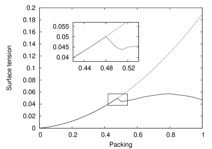
Figure 6: Surface tension $\beta\gamma a^{2}$ vs packing (system A). The dashed line describes values calculated for the isotropic phase. The inset shows the neighborhood of the point $y_{C}=0.48174$ with the transition from the isotropic phase to the biaxial nematic phase.

Figure 7: Surface tension $\beta\gamma a^{2}$ vs packing (system B). The dashed line describes values calculated for the isotropic phase. The inset shows the neighborhood of the point $y_{C}=0.29437$ with the transition from the isotropic phase to the biaxial nematic phase.

Figure 8: Comparison of the packing profiles $y(z)$ in the interfacial region for different phase packing in the bulk (system A).

Figure 9: Adsorption $\Gamma a^{2}$ vs packing for systems A and B.

V Summary

In this paper, we presented the statistical theory of hard molecules near a hard wall in the low-density Onsager approximation. A simple local approximation for the one-particle distribution function was applied. The theory was used to study two systems composed of the most biaxial hard spheroplatelets, where the direct transition from the isotropic phase to the biaxial nematic phase occurs in the bulk. The density and the order-parameter profiles near the wall were calculated.

The main result is the description of the phase near a wall at the transition from the isotropic to the biaxial nematic phase. Analytical results for the surface tension and the entropy contributions were presented. The results should not depend on the low-density approximation because they are the same for systems with different molecule elongations. The preferred orientation $(\vec{L},\vec{M},\vec{N})$ of the biaxial nematic phase is described by the condition $\vec{L}=\vec{e}_{z}$, where the short molecule axes tend to be perpendicular to the wall. The uniaxial symmetry along the axis perpendicular to the wall must be broken spontaneously in order to set the vectors $\vec{M}$ and $\vec{N}$. The phase orientation imposed by the wall extends into the bulk via the elastic forces.

For the case of the isotropic phase in the bulk, the phase near the wall is uniaxial because some orientations are excluded by the presence of the wall. The density profile of the phase in the interfacial region changes at the transition. If the phase is biaxial in the bulk then more molecules can enter the interfacial region. The complete wetting of the wall by a nematic film is not expected because the transition from the isotropic to the biaxial nematic phase is second order and the adsorption remains finite.

In order to confirm our predictions computer simulations of hard spheroplatelets near the wall are needed. It would be interesting to check the density profiles in the interfacial region. The validity of the local approximation for the one-particle distribution function could be also tested. We expect the short range density oscillations close to the wall.

Another interesting problem is the behavior of the system composed of less biaxial molecules where, on increasing the density, the following sequence of transitions is present: the first-order transition from the isotropic phase to the uniaxial nematic phase and, next, the second-order transition to the biaxial nematic phase.

- (1) M. J. Freiser, Phys. Rev. Lett. 24, 1041 (1970).
- (2) R. Berardi, L. Muccioli, S. Orlandi, M. Ricci, and C. Zannoni, J. Phys.: Condens. Matter 20, 463101 (2008).
- (3) C. Tschierske and D. J. Photinos, J. Mater. Chem. 20, 4263 (2010).
- (4) B. Jerome, Rep. Prog. Phys. 54, 391 (1991).
- (5) M. Kleman and O. D. Lavrentovich, Soft Matter Physics: An Introduction (Springer-Verlag, New York, 2003).
- (6) M. P. Allen, G. T. Evans, D. Frenkel, and B. M. Mulder, Adv. Chem. Phys. 86, 1 (1993).
- (7) M. P. Allen, Liq. Cryst. 8, 499 (1990).
- (8) D. Frenkel and B. M. Mulder, Mol. Phys. 55, 1171 (1985).
- (9) A. Stroobants, H. N. W. Lekkerkerker, D. Frenkel, Phys. Rev. A 36, 2929 (1987).
- (10) P. J. Camp and M. P. Allen, J. Chem. Phys. 106, 6681 (1997).
- (11) C. Vega, Mol. Phys. 92, 651 (1997).
- (12) A. N. Zakhlevnykh and P. A. Sosnin, Mol. Cryst. Liq. Cryst. 293, 135 (1997).
- (13) C. McBride and E. Lomba, Fluid Phase Equilib. 255, 37 (2007).
- (14) R. Berardi, C. Fava, and C. Zannoni, Chem. Phys. Lett. 236, 462 (1995).
- (15) R. Berardi, C. Fava, and C. Zannoni, Chem. Phys. Lett. 297, 8 (1998).
- (16) R. Berardi and C. Zannoni, J. Chem. Phys. 113, 5971 (2000).
- (17) C. Zannoni, J. Mater. Chem. 11, 2637 (2001).
- (18) R. Berardi, L. Muccioli, and C. Zannoni, J. Chem. Phys. 128, 024905 (2008).
- (19) B. S. John, C. Juhlin, and F. A. Escobedo, J. Chem. Phys. 128, 044909 (2008).
- (20) Y. Mart nez-Rat n, S. Varga, and E. Velasco, Phys. Chem. Chem. Phys. 13, 13247 (2011).
- (21) B. M. Mulder, Mol. Phys. 103, 1411 (2005).
- (22) G. S. Singh and B. Kumar, J. Chem. Phys. 105, 2429 (1996).
- (23) G. S. Singh and B. Kumar, Ann. Phys. (NY) 294, 24 (2001).
- (24) B. M. Mulder, Liq. Cryst. 1, 539 (1986).
- (25) B. Mulder, Phys. Rev. A 39, 360 (1989).
- (26) R. Holyst and A. Poniewierski, Mol. Phys. 69, 193 (1990).
- (27) M. P. Taylor, Liq. Cryst. 9, 141 (1991).
- (28) M. P. Taylor and J. Herzfeld, Phys. Rev. A 44, 3742 (1991).
- (29) E. van den Pol, A. V. Petukhov, D. M. E. Thies-Weesie, D. V. Byelov, and G. J. Vroege, Phys. Rev. Lett. 103, 258301 (2009).
- (30) A. G. Vanakaras, M. A. Bates, and D. J. Photinos, Phys. Chem. Chem. Phys. 5, 3700-3706 (2003).
- (31) S. Belli, A. Patti, M. Dijkstra, and R. van Roij, Phys. Rev. Lett. 107, 148303 (2011).
- (32) A. Kapanowski, Mol. Cryst. Liq. Cryst. 540, 50 (2011).
- (33) S. D. Peroukidis and A. G. Vanakaras, Soft Matter 9, 7419 (2013).
- (34) S. D. Peroukidis, A. G. Vanakaras, and D. J. Photinos, Phys. Rev. E 88, 062508 (2013).
- (35) W.-Y. Zhang, Y. Jiang, and J. Z. Y. Chen, Phys. Rev. Lett. 108, 057801 (2012).
- (36) M. M. Telo da Gama, Mol. Phys. 52, 585 (1984); 52, 611 (1984).
- (37) A. Poniewierski and R. Holyst, Phys. Rev. A 38, 3721 (1988).
- (38) A. Poniewierski, Phys. Rev. E 47, 3396 (1993).
- (39) R. Holyst and A. Poniewierski, Phys. Rev. A 38, 1527 (1988).
- (40) Y. Mao, P. Bladon, H. N. W. Lekkerkerker, and M. E. Cates, Mol. Phys. 92, 151 (1997).
- (41) R. van Roij, M. Dijkstra, and R. Evans, Europhys. Lett. 49, 350 (2000).
- (42) R. van Roij, M. Dijkstra, and R. Evans, J. Chem. Phys. 113, 7689 (2000).
- (43) M. Dijkstra, R. van Roij, and R. Evans, Phys. Rev. E 63, 051703 (2001).
- (44) M. Dijkstra and R. van Roij, J. of Phys.: Condens. Matter 17, S3507-S3514 (2005).
- (45) H. Reich, M. Dijkstra, R. van Roij, and M. Schmidt, J. Phys. Chem. B 111, 7825-7835 (2007).
- (46) A. Kapanowski, Phys. Rev. E 55, 7090 (1997).
- (47) R. Rosso and E. G. Virga, Phys. Rev. E 74, 021712 (2006).
- (48) W. H. Press, B. P. Flannery, S. A. Teukolsky, and W. T. Vetterling, Numerical Recipes in C: The Art of Scientific Computing (Cambridge University Press, Cambridge, 1988).
- (49) B. J. Berne and P. Pechukas, J. Chem. Phys. 56, 4213 (1972).
- (50) E. de Miguel and E. M. del Rio, J. Chem. Phys. 115, 9072 (2001).