On non-equilibrium photon distributions in the Casimir effect

Abstract

The electromagnetic field in a typical geometry of the Casimir effect is described in the Schwinger–Keldysh formalism. The main result is the photon distribution function (Keldysh Green function) in any stationary state of the field. A two-plate geometry with a sliding interface in local equilibrium is studied in detail, and full agreement with the results of Rytov fluctuation electrodynamics is found. As an illustration, plots are shown for a spectrum of the energy density between the plates.

I Introduction

In his seminal article 65 years ago, Casimir formulated a physical problem Cas which has had a tremendous influence on physics. His pioneering analysis of the physical consequences of field quantization under external, macroscopic boundary conditions is still of current relevance. Indeed, it turned out to be one of the most prolific ideas in modern theoretical physics. Having a pure quantum background and being closely related to classical physics, the Casimir effect is a universal and wide-spread phenomenon that can be found on all scales in the Universe.

One of the fascinating aspects of the Casimir effect is its simplicity, i.e., there are theoretical models that are amenable to exact solutions. Leaving aside many important features of modern Casimir physics Dalvit_Book , we consider the simple system of Ref.Cas with a slight generalization. Namely, our setting consists of two half-spaces of different materials with a plane-parallel gap in between. What we know about the two media are their reflection coefficients (a matrix in general) and macroscopic conditions like temperature distributions, macroscopic current densities, distance and relative motion parallel to the interfaces. We assume that these conditions are maintained stationary by external (generalized) forces. We want to compute correlation functions of the electromagnetic field in the gap. These yield for example the average energy density of the field and the pressure exerted on the two bodies as components of the stress (energy-momentum) tensor. We focus in particular on symmetrized correlations, also known as Keldysh-Green functions (KGF) in quantum kinetics, and are able to derive them under rather general circumstances in a stationary Casimir geometry. We thus establish a natural non-equilibrium extension of Casimir’s results.

Our approach starts from a simple observation which is a common feature among all manifestations of the Casimir effect: the interaction between the two interfaces disappears when their distance becomes large enough. On quite general grounds, we may therefore conclude that the electromagnetic field which we observe in any Casimir system results from several fields that originate in the material of the different half-spaces and in the vacuum gap between them. The distance dependence of the Casimir interaction is such that these fields become independent (uncorrelated) as the interfaces are infinitely far away. This fact is the cornerstone of our analysis: we use the large-distance limit to express the KGF in a two-plate setting in terms of KGFs of independent half-spaces.

In this paper, we relax the assumption that the two plates share the same temperature and state of motion. This makes it impossible to describe the field between the plates as being in thermal equilibrium. The appropriate tool to calculate photon correlation functions is then the Schwinger-Keldysh techniqueSchwinger_1961 ; Kel of nonequilibrium processes. The application of the Keldysh formalism to the field of Casimir-Van der Waals interactions has a relatively short history. The first application, to our knowledge, is due to Janowicz, Reddig and Holthaus Jan in calculations of the electromagnetic heat transfer between two bodies at different temperature. Sherkunov used the non-equilibrium technique extensively for dispersion interactions involving excited atoms and excited media Sher . A general expression for the electromagnetic force on an atom, in terms of the KGFs of atom and radiation field, was found a few years ago by one of the present authors vem .

The physical processes behind these field-mediated interactions are the multiple reflections of photons between the interfaces and their tunneling from one body to the other, which follow from the boundary conditions for the electromagnetic field on the interfaces. To include these boundary conditions, we use an effective action in the Schwinger-Keldysh technique with auxiliary fields and evaluate generating functionals for KGFs by performing path integrals NO . Path integral approaches for the Casimir effect were introduced by Bordag, Robaschik and Wieczorek Bord . Li and Kardar considered the interaction between bodies mediated by a fluid with long range correlations Meh2 ; Meh3 . They applied a path integral technique to include arbitrarily deformed bodies on which any kind of boundary condition can be implemented. This feature makes the approach amenable to a perturbative analysis of any deformed ideally conducting surfaces Emig1 ; Emig2 . Further on, Emig and Büscher Emig3 used the optical extinction theorem Born to reformulate the boundary conditions for a vacuum-dielectric interface in integral form that depends only on the fields on the vacuum side (i.e., in the gap between two bodies). They then derived with path integral techniques an effective Gaussian action for the photon gas in the gap, providing the free energy and in particular the Casimir interaction of dielectric bodies with arbitrary shaped surfaces. A similar approach has been followed by Soltan et al. Soltan for a dispersive medium between the bodies. Recently, Behunin and Hu applied path integrals to problems of the Casimir-Polder type (atom-surface interaction) in different nonequilibrium situations: in Ref.Hu1 is considered the Van der Waals interaction between an atom and a substrate in a stationary state out of global equilibrium; Ref.Hu2 is calculating atom-atom interactions in a quantized radiation field which is in a nonequilibrium state.

Our theoretical approach to the non-equilibrium Casimir interaction where the boundary conditions involve different, locally defined temperatures, is thus a synthesis between the Feynman path integral and the Keldysh-Schwinger formalism of nonequilibrium processes KL ; Alt .

The paper is organized as follows: after preliminary notations and introductions in Sec.II, we introduce rather general expressions for retarded Green functions in the Casimir geometry of two planar boundaries (Sec.III). In Sec.IV is analyzed a Gaussian action in Schwinger-Keldysh space which yields the non-equilibrium correlations for the fields (Keldysh-Green functions). This action implements in particular the boundary conditions for the retarded Green functions. In Sec.V we discuss the retarded Green functions in the limit where the interfaces of the Casimir system are infinitely removed from each other. Using this limiting procedure, the Keldysh-Green function at any point in the gap is expressed via Keldysh functions of the single interface systems defined at the surfaces and via photon numbers in free space (Sec.VI). As an application of the developed technique, we find in Sec.VII the field correlation functions in a Casimir geometry with a sliding interface. This result is checked in Appendix D where the same problem is solved using Rytov fluctuation electrodynamics. We illustrate our results by analyzing the electromagnetic energy density between the plates in two typical non-equilibrium situations (Appendix LABEL:a:energy-spectrum). Concluding remarks are given in Sec.VIII, while technical details are collected in the other Appendices.

II Preliminaries

II.1 Geometry of the problem

We consider two bodies with parallel and homogeneous boundaries located at $z=\pm a/2$. The boundaries are in stationary conditions: their temperatures are constant in time, and their relative motion (if any) is uniform and parallel to each other. We can then assume that the EM field in the cavity [$-a/2\leq z\leq a/2$] is stationary in time and homogenous in the $xy$-plane. As a consequence, all relevant fields and correlation functions can be expanded in Fourier integrals with respect to frequency $\omega$ and wave vectors ${\bf q}=(q_{x},q_{y})$ along the interfaces. We use in the following the shorthand

$$\Omega=(\omega,q_{x},q_{y})\,.$$ (II.1)

For fields like the vector potential, we get a mixed representation

$${\bf A}(\omega,q_{x},q_{y},z)={\bf A}(\Omega,z)\,,$$ (II.2)

where the argument $\Omega$ is suppressed where no confusion is possible.

We work in the Dzyaloshinskii gauge $\varphi=0$ where due to the transversality condition for the electric field, the normal component $A_{z}$ of the vector potential can be eliminated in favor of the tangential ones $A_{x},\,A_{y}$. Furthermore, given the plane of incidence spanned by ${\bf q}$ and the normal to the interfaces, the dynamical variables of the EM field in the cavity are the following linear combinations

$$A_{s}=\frac{q_{y}A_{x}-q_{x}A_{y}}{|{\bf q}|}\,,\qquad A_{p}=\frac{{\bf q}\cdot{\bf A}}{|{\bf q}|}\,,$$ (II.3)

which are nothing but the vector potential amplitudes of s- and p-polarized waves. In the following, we call the components defined in Eq.(II.3) the Weyl representation of the vector potential or we say the vector potential is written in the Weyl basis Pieplow_2012 : $\hat{A}=(A_{s},A_{p})$.

II.2 Weyl representation of free space Green function

The Green function (GF) of the EM field plays a crucial role in the following. Since it simply represents the vector potential due to a point current source, it is also represented by a mixed Fourier representation involving a tensor $D_{\alpha\alpha^{\prime}}(\Omega;z,z^{\prime})$ ($\alpha,\alpha^{\prime}=x,y,z$). The latter is the solution of (given the gauge $\varphi=0$) Landau_9

$$\left[(\partial_{z}^{2}+q_{z}^{2})\delta_{\alpha\beta}-{\partial}_{\alpha}{\partial}_{\beta}\right]D_{\beta\alpha^{\prime}}(\Omega;z,z^{\prime})=4\pi\delta_{\alpha\alpha^{\prime}}\delta(z-z^{\prime})$$ (II.4)

where (we set $c=1$)

$$q_{z}^{2}=\omega^{2}-q^{2}\,,\quad{\partial}_{\alpha}=(iq_{x},iq_{y},\partial_{z})$$ (II.5)

In the following, we only need the tangential part of the GF $D_{\sigma\sigma^{\prime}}$ with $\sigma,\sigma^{\prime}=x,y$. (See Eqs.(III.16–III.18) below for the normal components.) Projecting both indices into the Weyl basis according to Eq.(II.3), we get from Eq.(II.4) the simple Helmholtz equation

$$(\partial_{z}^{2}+q_{z}^{2})\hat{D}(\Omega;z,z^{\prime})=4\pi\hat{g}\delta(z-z^{\prime}),$$ (II.6)

where the $2\times 2$ matrix $\hat{g}$ reads

$$\hat{g}=\left(\begin{array}[]{cc}1&0\\ 0&q_{z}^{2}/\omega^{2}\end{array}\right)\,.$$ (II.7)

The GF in free space (no boundary conditions) is written $\hat{\Delta}(\Omega;z,z^{\prime})$. As is well known, it comes in two types: retarded $\hat{\Delta}^{R}$ and advanced $\hat{\Delta}^{A}$ Green functions. In the Weyl representation, they are given by

$$\hat{\Delta}^{R}(\Omega;z,z^{\prime})=\hat{\Delta}_{0}\,{\rm e}^{iq_{z}|z-z^{\prime}|}=\hat{\Delta}^{A\ast}(\Omega;z,z^{\prime})$$ (II.8)

where

$$\hat{\Delta}_{0}=\frac{2\pi}{iq_{z}}\hat{g}$$ (II.9)

and the wave vector $q_{z}$ is defined over the entire frequency axis by

$$q_{z}=\left\{\begin{array}[]{ll}\mathop{\rm sgn}\omega\sqrt{\omega^{2}-q^{2}}+i0&\mbox{for}\quad\omega^{2}>q^{2}\\ i\sqrt{q^{2}-\omega^{2}}&\mbox{for}\quad q^{2}>\omega^{2}\end{array}\right.$$ (II.10)

The two cases corresponding to outgoing propagating and to evanescent waves, respectively. The infinitesimal imaginary part of $q_{z}$ in (II.10) secures the analytical continuation of $\hat{\Delta}^{R}$ to complex frequencies in the upper half plane. It entails the existence of the limit

$$\lim_{a\to+\infty}{\rm e}^{iq_{z}a}=0$$ (II.11)

for both propagating and evanescent waves. In addition, we have the symmetry relation

$$q_{z}(-\Omega)=-q_{z}^{*}(\Omega)\,.$$ (II.12)

As a consequence, the retarded GF has the property $\hat{\Delta}^{R}(-\Omega;z,z^{\prime})=\hat{\Delta}^{R\ast}(\Omega;z,z^{\prime})$, as it should, being a response function between real-valued fields.

III Retarded Green functions

III.1 Single interface

We include stationary and translation-invariant (in the $xy$-plane) boundary conditions in the retarded GF by adding reflected waves. Let us start with a single interface at $z=-a/2$ where the GF (subscript $-$) reads

$$\hat{D}_{-}^{R}(\Omega;z,z^{\prime})=\hat{\Delta}^{R}(\Omega;z,z^{\prime})+\hat{R}_{-}\hat{\Delta}_{0}\,{\rm e}^{iq_{z}(z+z^{\prime}+a)},$$ (III.1)

for $z,z^{\prime}\geq-a/2$. The first term is the same as in free space. The reflection matrix $\hat{R}_{-}$ at the lower interface takes a simple diagonal form in the frame where the lower body is at rest

$$\hat{R}_{-}=\left(\begin{array}[]{cc}R^{s}_{-}&0\\ 0&R^{p}_{-}\end{array}\right)$$ (III.2)

whose matrix elements are for a

$$\mbox{metal}:\quad R^{s}_{-}=\frac{q_{z}\zeta(\omega)-\omega}{q_{z}\zeta(\omega)+\omega}\,,\quad R^{p}_{-}=\frac{\omega\zeta(\omega)-q_{z}}{\omega\zeta(\omega)+q_{z}}\,,$$ (III.3)

where $\zeta(\omega)$ is the (dimensionless) impedance, and for a

$$\mbox{dielectric}:\quad R^{s}_{-}=\frac{q_{z}-q_{z\varepsilon}}{q_{z}+q_{z\varepsilon}}\,,\quad R^{p}_{-}=\frac{q_{z\varepsilon}-\varepsilon(\omega)q_{z}}{q_{z\varepsilon}+\varepsilon(\omega)q_{z}}\,,$$ (III.4)

where $\varepsilon(\omega)$ is the dielectric permittivity and

$$q_{z\varepsilon}=[\varepsilon(\omega)\omega^{2}-q^{2}]^{1/2}$$ (III.5)

the wave vector in the lower medium.

If only the upper medium is present, we have a GF similar to Eq.(III.1), for $z,z^{\prime}\leq+a/2$

$$\hat{D}_{+}^{R}(\Omega;z,z^{\prime})=\hat{\Delta}^{R}(\Omega;z,z^{\prime})+\hat{R}_{+}\hat{\Delta}_{0}\,{\rm e}^{-iq_{z}(z+z^{\prime}-a)}\,,$$ (III.6)

where $\hat{R}_{+}$ is the corresponding reflection matrix. We suppose here a generic form for $\hat{R}_{+}$. The case of a sliding upper interface is discussed in Appendix D.

III.2 General properties

Let us collect a few general properties of the reflection matrices and the GFs. It follows from Eq.(D.17–D.20) for $\hat{R}_{+}$ and from the diagonal form of $\hat{R}_{-}$ [Eq.(III.2)] that both fulfill the identity

$$\hat{g}\hat{R}_{\nu}^{T}=\hat{R}_{\nu}\hat{g}\,,\quad\nu=\pm$$ (III.7)

The retarded GF (III.1) therefore satisfies

$$\hat{D}^{R}(\Omega;z,z^{\prime})=[\hat{D}^{R}(\Omega;z^{\prime},z)]^{T}$$ (III.8)

which is not the reciprocity condition because the wave vector $\mathbf{q}$ in the arguments of both sides is the same.

Taking into account Eqs.(II.12) and (D.17–D.20), the reflection matrices in Eq.(III.2) and Sec.D satisfy the identity

$$\hat{R}_{\nu}(-\Omega)=\hat{R}_{\nu}^{\ast}(\Omega)$$ (III.9)

where the asterisk denotes the element-wise complex conjugation. This entails that the symmetry relation is also valid for the retarded GF at a single interface

$$\hat{D}^{R}_{\nu}\left(-\Omega;z,z^{\prime}\right)=\hat{D}^{R\ast}_{\nu}\left(\Omega;z,z^{\prime}\right)\,,\quad\nu=\pm$$ (III.10)

Below, we shall also deal with the advanced GF which is defined as

$$\hat{D}^{A}_{\nu}(\Omega;z,z^{\prime})=[\hat{D}^{R}_{\nu}(\Omega;z^{\prime},z)]^{\dagger}=\hat{D}^{R\ast}_{\nu}(\Omega;z,z^{\prime})$$ (III.11)

where the last equality follows from Eq.(III.8).

III.3 Planar cavity

The preceding properties carry over to the retarded and advanced GF in the cavity formed by two interfaces. By adding up multiply reflected waves, one finds the expression

$$\hat{D}^{R}(\Omega;z,z^{\prime})=\hat{\Delta}^{R}(\Omega;z,z^{\prime})+\sum\limits_{\nu,\nu^{\prime}=\pm}\hat{C}^{\nu\nu^{\prime}}\,{\rm e}^{iq_{z}(\nu z+\nu^{\prime}z^{\prime})}$$ (III.12)

where

$$\hat{C}^{--}=\hat{U}_{+-}^{-1}\hat{R}_{+}\hat{\Delta}_{0}\,{\rm e}^{iq_{z}a}\,,\quad\hat{C}^{-+}=\hat{U}_{+-}^{-1}\hat{R}_{+}\hat{R}_{-}\hat{\Delta}_{0}\,{\rm e}^{2iq_{z}a}$$ (III.13)

and $\hat{C}^{++},\hat{C}^{+-}$ are defined by swapping indices $-\leftrightarrow+$ in Eq.(III.13). The matrix $\hat{U}_{+-}$ takes into account multiple reflections of photons in the cavity; it is given by the expression

$$\hat{U}_{+-}=\hat{I}-\hat{R}_{+}\hat{R}_{-}\,{\rm e}^{2iq_{z}a}\,,$$ (III.14)

where $\hat{I}$ is the unit matrix. An analogous formula gives $\hat{U}_{-+}$. Eq.(III.7) above gives us the property

$$\hat{U}_{-+}^{-1}\hat{g}=\hat{g}\hat{U}_{+-}^{-1T}$$ (III.15)

which ensures that the generalized reciprocity relation (III.8) also holds for the cavity GF (III.12). Similarly, the relation (III.11) between retarded and advanced GFs remains true as well.

III.4 Normal components

To conclude this Section, we give the tensor components involving the normal direction. The following formulas can be shown from the wave equation Eq. (II.4) and the symmetry properties above ($\lambda=s,p$ and $q=|{\bf q}|$):

$$q_{z}^{2}D_{z\lambda}^{R} = iq\partial_{z}D_{p\lambda}^{R}\,,$$ (III.16)

$$q_{z}^{2}D_{\lambda z}^{R} = -iq\partial_{z^{\prime}}D_{\lambda p}^{R}\,,$$ (III.17)

$$q_{z}^{2}D_{zz}^{R} = \frac{q^{2}}{q_{z}^{2}}\partial_{z}\partial_{z^{\prime}}D_{pp}^{R}+4\pi\delta(z-z^{\prime})\,.$$ (III.18)

III.5 Generalized impedance matrices

The reflection matrices $\hat{R}_{\nu}$ appearing in the expressions above are the solutions to a scattering problem at the planar interfaces. We discuss here an equivalent formulation in terms of generalized surface impedances. These will provide the link between boundary conditions imposed on fields and interactions with auxiliary fields restricted to the interfaces.

Evaluating the derivative with respect to $z$ and $z^{\prime}$ of the retarded GF (III.12) at the interfaces $\pm a/2$, we come to the boundary conditions. With respect to the first coordinate $z$ (derivative $\partial_{z}$), we find

$$iq_{z}^{-1}\partial_{z}\hat{D}^{R}(-a/2,z^{\prime})-\hat{Y}_{-}\hat{D}^{R}(-a/2,z^{\prime})=0\quad$$ (III.19)

$$iq_{z}^{-1}\partial_{z}\hat{D}^{R}(+a/2,z^{\prime})+\hat{Y}_{+}\hat{D}^{R}(+a/2,z^{\prime})=0$$ (III.20)

where we defined the matrices

$$\hat{Y}_{\nu}=(\hat{I}+\hat{R}_{\nu})^{-1}(\hat{I}-\hat{R}_{\nu})\,,\quad\nu=\pm$$ (III.21)

These generalize the concept of a surface admittance to a general reflection problem. Indeed, from the reflection amplitudes (III.3) for a metallic surface at rest, we get in the Weyl basis

$$\mbox{metal:}\quad\hat{Y}_{-}=\frac{1}{\zeta(\omega)}\left(\begin{array}[]{cc}\omega/q_{z}&0\\ 0&q_{z}/\omega\end{array}\right)$$ (III.22)

Note that despite multiple reflections, the boundary conditions (III.19, III.20) are of local character: they link the fields and their normal derivatives at the same position with the corresponding admittance matrices.

With respect to the second coordinate $z^{\prime}$ (derivative $\partial_{z^{\prime}}$) of the GF, a similar calculation yields

$$iq_{z}^{-1}\partial_{z^{\prime}}\hat{D}^{R}(z,{-a/2})-\hat{D}^{R}(z,-a/2)\hat{Y}_{-}^{T}=0\quad$$ (III.23)

$$iq_{z}^{-1}\partial_{z^{\prime}}\hat{D}^{R}(z,{+a/2})+\hat{D}^{R}(z,+a/2)\hat{Y}_{+}^{T}=0$$ (III.24)

where the admittance matrices appear transposed.

In the case of a single interface, we still find two boundary conditions at $z,z^{\prime}=\pm a/2$. If the “missing” body is the upper one, for example, the admittance degenerates into $\hat{Y}_{+}=\hat{I}$ from Eq.(III.21). The boundary condition (III.20) then becomes equivalent to the Sommerfeld condition for an outgoing wave: $\hat{D}^{R}(z,z^{\prime})\sim{\rm e}^{iq_{z}z}$. This holds as long as $z>z^{\prime}$ and in both the propagating and evanescent sectors.

III.6 Remarkable identity

Using the boundary conditions (III.19–III.24), their counterparts for the advanced GF $\hat{D}^{A}$, and the Green equation (II.6), we come to the following property of the GFs in the two-plate geometry

$$\sum\limits_{\nu=\pm} \hat{D}^{R}(z,\nu a/2)\hat{\Gamma}^{\nu}\hat{D}^{A}(\nu a/2,z^{\prime})$$ (III.25)

$$=\hat{D}^{R}(z,z^{\prime})-\hat{D}^{A}(z,z^{\prime})$$

In Eq.(III.25) we have introduced effective source strengths

$$\hat{\Gamma}^{\nu}=-\frac{1}{2}\left(\hat{\Delta}_{0}^{-1}\hat{Y}_{\nu}-\mbox{h.c.}\right)$$ (III.26)

which are easily shown to be antihermitian: $\hat{\Gamma}^{\nu\dagger}=-\hat{\Gamma}^{\nu}$ and symmetric: $\hat{\Gamma}^{\nu T}=\hat{\Gamma}^{\nu}.$ Therefore, they have purely imaginary matrix elements: $\hat{\Gamma}^{\nu\ast}=-\hat{\Gamma}^{\nu}.$ Besides, using the parity properties (II.12) and (III.9) of $q_{z}$ and the reflection matrices, the definition of the $\hat{\Gamma}^{\nu}$ entails

$$\hat{\Gamma}^{\nu}(-\Omega)=\hat{\Gamma}^{\nu\ast}(\Omega)=-\hat{\Gamma}^{\nu}(\Omega)$$ (III.27)

The identity (III.25) has a long history in macroscopic fluctuation electrodynamics. It has been noted by Eckhardt Eckhardt_1982 , although involving a spatial integral over volumes where the imaginary part of the permittivity is nonzero. The version we give here is technically somewhat simpler because only surface sources appear. This may be related to the “holographic principle” stating that under certain circumstances, all relevant properties of a (source-free) field are encoded in a hypersurface. This is obviously related to the classical Huyghens principle. An alternative proof of Eq.(III.25) is given in Appendix A using the Leontovich surface impedance boundary condition.

If one of the two interfaces is missing, an identity similar to Eq.(III.25) can be derived analogously. One simply has to replace the source strength for the missing interface by

$$\Gamma^{\nu}\mapsto\Gamma^{0}=-\frac{1}{2}\left(\hat{\Delta}_{0}^{-1}\hat{I}-\mbox{h.c.}\right)=-\hat{\Delta}_{0}^{-1}\Theta(\omega^{2}-q^{2})$$ (III.28)

where $\Theta$ is the unit step function. Note that only propagating waves appear on the free boundary: they represent the fields incident from infinity towards the interface.

IV Non-equilibrium action

We now address the key problem of this paper: evaluate correlations for the EM field under non-equilibrium conditions. To this effect, we use the path integral method and work with an action for the EM field. An auxiliary field $\varphi$ is introduced to enforce the boundary conditions at the two interfaces NO . This technique was developed in previous work Bord ; Meh2 ; Meh3 for equilibrium situations. We extend the approach to the whole Schwinger-Keldysh space and define a Gaussian action for two coupled Bose fields: the vector potential $A$ and the auxiliary field $\varphi$

$$S = \frac{1}{2}\int\big{\{}\check{A}^{{\dagger}}(\Omega,z)\check{\Delta}^{-1}(\Omega;z,z^{\prime})\check{A}(\Omega,z^{\prime})+\check{\varphi}^{{\dagger}}(\Omega)\check{F}\check{\varphi}(\Omega)$$

$$+\check{\varphi}^{{\dagger}}(\Omega)\check{M}(\Omega,z)\check{A}(\Omega,z)+\check{A}^{{\dagger}}(\Omega,z)\check{M}^{{\dagger}}(\Omega,z)\check{\varphi}(\Omega)\big{\}}\,.$$

The integration is over $\Omega$ and $z$. In the action (LABEL:eq:6.1), the vector potential $\check{A}$ lives in Keldysh space and has two components that are called quantum $\hat{A}^{\rm q}$ and classical $\hat{A}^{\rm cl}$:

$$\check{A}=\left(\begin{array}[]{c}\hat{A}^{\rm q}\\ \hat{A}^{\rm cl}\end{array}\right)\,,$$ (IV.2)

each of which contains the familiar transverse amplitudes in the Weyl basis

$$\hat{A}=\left(\begin{array}[]{c}A_{s}\\ A_{p}\end{array}\right)\,.$$ (IV.3)

The $4\times 4$ matrix $\check{\Delta}^{-1}$ is the inverse of the Keldysh-Green (KG) matrix of the free EM field. In the Keldysh basis (IV.2) for $\check{A}$, this KG matrix has the block structure

$$\check{\Delta}=\left(\begin{array}[]{cc}\hat{0}&\hat{\Delta}^{A}\\ \hat{\Delta}^{R}&\hat{\Delta}^{K}\end{array}\right)\,,$$ (IV.4)

where $\hat{\Delta}^{R,A}$ are the retarded and advanced Green functions for free space, introduced in Sec.II.2. The function $\hat{\Delta}^{K}$ is the KGF for the free field, it collects symmetrized correlations of the vector potential. (A calculation is sketched in Sec.C below.) Our goal is to calculate its counterpart in the presence of the two interfaces that we denote $\hat{D}^{K}$. It is given in the coordinate representation X as ($x=(t,{\bf r})$)

$$D_{\alpha\alpha^{\prime}}^{K}(x,x^{\prime})=-i\left\langle\{\hat{A}_{\alpha}(x),\hat{A}_{\alpha^{\prime}}(x^{\prime})\}_{+}\right\rangle$$ (IV.5)

where $\{\cdot,\,\cdot\}_{+}$ is the anti-commutator. We work here with the corresponding Fourier transforms with respect to $t-t^{\prime}$ and to the tangential coordinates. In the Weyl basis, this gives the matrix $\hat{D}^{K}(\Omega,z,z^{\prime})$.

The auxiliary field $\check{\varphi}$ in Eq.(LABEL:eq:6.1) has eight components that are also grouped in the Keldysh structure

$$\check{\varphi}=\left(\begin{array}[]{c}\hat{\varphi}^{\rm q}\\ \hat{\varphi}^{\rm cl}\end{array}\right)\,.$$ (IV.6)

The components $\hat{\varphi}^{\rm q,\,cl}$ themselves are

$$\hat{\varphi}=\left(\begin{array}[]{c}\varphi_{-,s}\\ \varphi_{-,p}\\ \varphi_{+,s}\\ \varphi_{+,p}\end{array}\right)\,.$$ (IV.7)

They are Weyl spinors localized in the lower (index $-$) and the upper ($+$) interface. Finally, the matrix $\check{M}(\Omega,z)$ in the action (LABEL:eq:6.1) is related, as we shall see below, to the boundary conditions imposed at $z=\pm a/2$.

IV.1 Evaluating the path integral

We follow the standard path integral procedure and add source terms to the action (LABEL:eq:6.1)

$$\frac{1}{2}\int(\check{J}^{{\dagger}}\check{A}+\check{A}^{{\dagger}}\check{J})$$ (IV.8)

Then Gaussian path integrals are evaluated, first over the EM field and then over the auxiliary field. We get the generating functional for field correlations whose expansion to second order in $\check{J}$ provides the following expression for the KG matrix:

$$\check{D}=\check{\Delta}+\check{\Delta}\check{M}^{{\dagger}}\check{\Lambda}\check{M}\check{\Delta}$$ (IV.9)

where $\check{\Lambda}$ is the solution of

$$\check{\Lambda}^{-1}=\check{F}-\check{M}\check{\Delta}\check{M}^{{\dagger}}$$ (IV.10)

The KG matrix $\check{D}$ of Eq.(IV.9) must have the block structure (IV.4) with off-diagonal blocks that are Hermitian conjugates [Eq.(III.11)] and with an antihermitian Keldysh block

$$[\hat{D}^{K}(\Omega;z,z^{\prime})]^{{\dagger}}=-\hat{D}^{K}(\Omega;z^{\prime},z)\,.$$ (IV.11)

In addition, we impose the boundary conditions (III.19–III.24) on the off-diagonal elements $\hat{D}^{R},\hat{D}^{A}$ of (IV.9). These conditions unambiguously define the structure of the matrices $\check{M}$ and $\check{F}$ in the action (LABEL:eq:6.1) as

$$\check{F}=\left(\begin{array}[]{cc}\hat{F}&\hat{0}\\ \hat{0}&\hat{0}\end{array}\right)$$ (IV.12)

where $\hat{F}$ is a $4\times 4$ antihermitian matrix, and

$$\check{M}=\left(\begin{array}[]{cc}\hat{0}&\hat{M}\\ \hat{M}^{\ast}&\hat{0}\end{array}\right)$$ (IV.13)

Here the matrix $\hat{M}$ collects the boundary conditions at the two interfaces into a vector of operators in the Weyl basis

$$\hat{M}(\Omega,z)=\left(\begin{array}[]{c}\delta(z+a/2)[iq_{z}^{-1}\hat{I}\partial_{z}-\hat{Y}_{-}]\\ \delta(z-a/2)[iq_{z}^{-1}\hat{I}\partial_{z}+\hat{Y}_{+}]\end{array}\right)$$ (IV.14)

The boundary conditions (III.19–III.20) then take the integral form (common argument $\Omega$ suppressed)

$$0 = \int\!dz\,\hat{M}(z)\hat{D}^{R}(z,z^{\prime})$$ (IV.15)

$$0 = \int\!dz^{\prime}\,\hat{D}^{R}(z,z^{\prime})\hat{M}^{T}(z^{\prime})$$ (IV.16)

with a derivative $\partial_{z^{\prime}}$ acting to the left in the second line. For the advanced GF, the boundary conditions (III.23–III.24) can be written as integrals over $\hat{M}^{\ast}(z)\hat{D}^{A}(z,z^{\prime})$ and over $\hat{D}^{A}(z,z^{\prime})\hat{M}^{{\dagger}}(z^{\prime})$.

With the choices (IV.12, IV.13), one can show that the Keldysh action (LABEL:eq:6.1) acquires that so-called “causal structure” KL ; Alt .

Inserting the matrices $\check{M}$ and $\check{F}$ from Eqs.(IV.13, IV.12) into Eq.(IV.9), we find for the KG functions $\hat{D}^{R,A,K}$ the expressions

$$\hat{D}^{R} = \hat{\Delta}^{R}+\hat{\Delta}^{R}\hat{M}^{T}\hat{\Lambda}\hat{M}\hat{\Delta}^{R}$$ (IV.17)

$$\hat{D}^{A} = \hat{\Delta}^{A}+\hat{\Delta}^{A}\hat{M}^{{\dagger}}\hat{\Lambda}^{{\dagger}}\hat{M}^{\ast}\hat{\Delta}^{A}$$ (IV.18)

$$\hat{D}^{K} = \big{(}\hat{I}+\hat{\Delta}^{R}\hat{M}^{T}\hat{\Lambda}\hat{M}\big{)}\hat{\Delta}^{K}\big{(}\hat{I}+\hat{M}^{{\dagger}}\hat{\Lambda}^{{\dagger}}\hat{M}^{\ast}\hat{\Delta}^{A}\big{)}$$ (IV.19)

$${}+\hat{\Delta}^{R}\hat{M}^{T}\hat{\Lambda}\hat{F}\hat{\Lambda}^{{\dagger}}\hat{M}^{\ast}\hat{\Delta}^{A}$$

where $\hat{\Lambda}$ is a $4\times 4$ matrix given by

$$\hat{\Lambda}=-(\hat{M}\hat{\Delta}^{R}\hat{M}^{T})^{-1}$$ (IV.20)

The expressions (IV.17) and (IV.18) are integral forms of retarded and advanced GF because matrix products actually have to be read as the concatenation of integral operators. It is trivial to check that they satisfy the boundary conditions (IV.15, IV.16). Using the explicit form (IV.14) of $\hat{M}$, we have checked in a straightforward calculation that Eq.(IV.17) coincides with Eq.(III.12) for the retarded GF.

IV.2 Distribution (Keldysh-Green) functions for photons

To analyse the expression (IV.19) for the KG function, we first observe that the first term is equal to zero because $\hat{\Delta}^{K}$ is a solution of the homogeneous equation corresponding to Eq.(II.6). (See Appendix B for details.) We shall argue that $\hat{F}$ that characterizes the auxiliary fields can be taken in block-diagonal form

$$\hat{F}=\left(\begin{array}[]{cc}4\hat{\Delta}_{0}\hat{P}(-)\hat{\Delta}_{0}^{{\dagger}}&\hat{0}\\ \hat{0}&4\hat{\Delta}_{0}\hat{P}(+)\hat{\Delta}_{0}^{{\dagger}}\end{array}\right)$$ (IV.21)

where the quantity $\hat{P}(-)$ [$\hat{P}(+)$] correspond to the lower [upper] boundary, respectively. Adopting this choice, a tedious, but elementary calculation leads us to (common argument $\Omega$ suppressed)

$$\hat{D}^{K}(z,z^{\prime})=\sum\limits_{\nu=\pm}\hat{D}^{R}(z,\nu a/2)\hat{P}(\nu)\hat{D}^{A}(\nu a/2,z^{\prime})\,,$$ (IV.22)

for the KG function. This has the same form as the Keldysh equation in quantum kinetics Kel . If we would take this formal analogy serious, then the quantities $\hat{P}(\Omega;\nu)$ would coincide with the Keldysh polarization operators on the boundaries (i.e., the KG correlation of interface polarization fields). In the non-equilibrium theory, these are nonlinear functionals of the Keldysh function for photons, so that in the semiclassical approximation, Eq.(IV.22) would generate a kinetic equation of Boltzmann type for the photon distribution function.

In the two-plate geometry of the Casimir effect, however, this is not the case because the $\hat{P}(\nu)$ are independent of the photon KG functions $\hat{D}^{R}$, $\hat{D}^{A}$, and $\hat{D}^{K}$. They are rather determined by given macroscopic states of the bodies and their interfaces and act like a linear driving for the EM field in the cavity. This suggests an interpretation of Eq.(IV.22) in the spirit of Rytov’s fluctuation electrodynamics: the quantities $\hat{P}(\pm)$ encapsulate the distribution of photon sources. They are the only piece of information needed to produce the (non-equilibrium) distribution function of photons in the cavity. For this reason, we call $\hat{P}(\pm)$ the photon sources or fluctuating sources in the following.

The above interpretation also helps to understand the diagonal form for the source distribution function $\hat{F}$ in Eq.(IV.21): the sources are located on the bodies’ interfaces, and correlations between the macroscopic states of the two bodies are neglected. We intend to investigate corrections to this approximation in future work.

V The large distance limit

In this Section, we consider the limit $a\to\infty$ in order to fix the strength of photon sources by referring to the EM field in free space and near a single interface.

There are three different ways to take the limit:

(A) If we fix both points $z$, $z^{\prime}$ in the cavity and go to the limit $a\to\infty$, we recover Green functions in free space. In particular for the retarded Green function,

$$\lim\limits_{a\to\infty}\hat{D}^{R}(z,z^{\prime})=\hat{\Delta}^{R}(z,z^{\prime})$$ (V.1)

with the free space Green function defined in Eq.(II.8).

(B) If the points stay at fixed distances $z,z^{\prime}>0$ from the lower interface, we get

$$\lim\limits_{a\to\infty}\hat{D}^{R}(z-a/2,z^{\prime}-a/2)=\hat{D}^{R}_{-}(z,z^{\prime};a\to 0)\equiv\hat{d}^{R}_{-}(z,z^{\prime})$$ (V.2)

where $\hat{D}^{R}_{-}$ is the Green function above a single interface. The notation $(\ldots;a\to 0)$ means that in the expression for $\hat{D}^{R}_{-}$ [Eq.(III.1)], $a$ should be set to zero.

(C) Similarly, we may take points at positions $z,z^{\prime}<0$ below the upper interface and get the Green function below a single interface:

$$\lim\limits_{a\to\infty}\hat{D}^{R}(z+a/2,z^{\prime}+a/2)=\hat{D}^{R}_{+}(z,z^{\prime};a\to 0)\equiv\hat{d}^{R}_{+}(z,z^{\prime})$$ (V.3)

where the Green function $\hat{D}^{R}_{+}(z,z^{\prime};a\to 0)$ is defined similar to case (B) from Eq.(III.6).

We also need for the Keldysh-Green function Eq.(IV.22) the limiting values when one position in the Green functions recedes to infinity. Keeping $z$ fixed,

$${a\to\infty}:\quad \hat{D}^{R}(z,\nu a/2)\to\hat{\Delta}^{R}(z,\nu)\,{e}^{iq_{z}a/2}\,,$$ (V.5)

$$\hat{\Delta}^{R}(z,\nu)=\hat{\Delta}_{0}\,{e}^{-i\nu q_{z}z}$$

In this limit, the exponential ${\rm e}^{iq_{z}a/2}$ in the first line restricts the support to propagating waves (real $q_{z}$); it drops out when products with the advanced GF $\hat{D}^{A}$ are formed because of Eq.(II.8). In a similar way, we define for the single-interface limits (B, C) the functions

$$\hat{d}_{-}^{R}(z,\nu) = [\hat{I}e^{-i\nu q_{z}z}+\hat{R}_{-}e^{iq_{z}z}]\hat{\Delta}_{0}$$ (V.6)

$$\hat{d}_{+}^{R}(z,\nu) = [\hat{I}e^{-i\nu q_{z}z}+\hat{R}_{+}e^{-iq_{z}z}]\hat{\Delta}_{0}$$ (V.7)

VI Keldysh–Green functions

We now consider the KG function derived at Eq.(IV.22) in the limit $a\rightarrow+\infty$ in order to find the photon sources $\hat{P}(\nu)$. Using the notation $\hat{\Delta}^{K}$, $\hat{d}_{\pm}^{K}$ and $\hat{P}_{0,-,+}$ in the three limits (A), (B) and (C), we get

$$\hat{\Delta}^{K}(z,z^{\prime}) = \sum\limits_{\nu}\hat{\Delta}^{R}(z,\nu)\hat{P}_{0}(\nu)\hat{\Delta}^{A}(\nu,z^{\prime})\,,$$ (VI.1)

$$\hat{d}_{\mp}^{K}(z,z^{\prime}) = \sum\limits_{\nu}\hat{d}_{\mp}^{R}(z,\nu)\hat{P}_{\mp}(\nu)\hat{d}_{\mp}^{A}(\nu,z^{\prime})\,,$$ (VI.2)

where the GFs on the right hand sides are defined in Eqs.(V.5–V.7) above. Manifestly, the sources in free space $\hat{P}_{0}(\nu)$ are defined by the quantum state of free EM field. Similarly, the fluctuation sources on the physical interfaces [the lower one, $\hat{P}_{-}(-)$ in case (B) and the upper one, $\hat{P}_{+}(+)$ in case (C)] are defined by the macroscopic quantum state of the corresponding bodies.

We assume the statistical independence of the bodies and the free EM field Henkel_2002 and come to the conclusion that the sources on the ‘free interfaces’ coincide:

$$\hat{P}_{-}(+)=\hat{P}_{0}(+)\,;\quad\hat{P}_{+}(-)=\hat{P}_{0}(-)\,,$$ (VI.3)

and that the sources on the macroscopic interfaces are the same for one and for two plates:

$$\hat{P}(-)=\hat{P}_{-}(-)\,;\quad\hat{P}(+)=\hat{P}_{+}(+)\,.$$ (VI.4)

By evaluating Eq.(VI.2) at $z=z^{\prime}=0$, we can also express the interface sources in terms of the KG function there:

$$\hat{P}(\nu)=\hat{\Delta}_{0}^{-1}(\hat{I}+\hat{R}_{\nu})^{-1}\hat{d}_{\nu}^{K}(\hat{I}+\hat{R}_{\nu}^{\dagger})^{-1}\hat{\Delta}_{0}^{-1\dagger}-\hat{P}_{0}(-\nu)$$ (VI.5)

where $\hat{d}_{\nu}^{K}$ is the boundary value of the KG function for a system with a single interface

$$\hat{d}_{\nu}^{K}=\hat{d}_{\nu}^{K}(\Omega;0,0)$$ (VI.6)

The free space photon sources $\hat{P}_{0}(\nu)$ are calculated in Appendix C. In Sec.VII, we work out the quantities $\hat{P}(\nu)$ for a specific example, allowing for the upper body to be in uniform motion relative to the lower one.

We are now ready to collect our main result. The explicit expressions for the GFs $\hat{D}^{R,A}$ [Eqs.(III.1, III.11)] and for the photon sources $\hat{P}$ [Eq.(VI.4)] are inserted into the KG function (IV.22) to give

$$\hat{D}^{K}(z,z^{\prime})=\sum\limits_{\nu,\nu^{\prime}=\pm}\hat{D}^{\nu\nu^{\prime}}e^{i(\nu q_{z}z-\nu^{\prime}q_{z}^{\ast}z^{\prime})}\,.$$ (VI.7)

We find the amplitudes

$$\hat{D}^{--} = \hat{T}_{+}+e^{-2{\rm Im}\,q_{z}a}\hat{R}_{+}\hat{T}_{-}\hat{R}_{+}^{\dagger}\,,$$ (VI.8)

$$\hat{D}^{-+} = \hat{R}_{+}\hat{T}_{-}e^{iq_{z}a}+\hat{T}_{+}\hat{R}_{-}^{\dagger}e^{-iq_{z}^{\ast}a}\,,$$ (VI.9)

$$\hat{T}_{-} = \hat{U}_{-+}^{-1}\hat{\gamma}_{-}\hat{U}_{-+}^{-1\dagger}\,;$$ (VI.10)

where $\hat{D}^{++}$, $\hat{D}^{+-}$, $T_{+}$ are found by swapping the subscripts $+$ and $-$, $\hat{U}_{-+}$ has been defined in Eq.(III.14), and

$$\hat{\gamma}_{\nu}=e^{-{\rm Im}\,q_{z}a}(\hat{I}+\hat{R}_{\nu})\hat{\Delta}_{0}\hat{P}(\nu)\hat{\Delta}_{0}^{\dagger}(\hat{I}+\hat{R}_{\nu}^{\dagger})$$ (VI.11)

These expressions give the distribution function of photons in a planar cavity (homogeneous along the $xy$-directions and stationary in time) whatever the macroscopic state of the two boundaries, as encoded in $\hat{P}(\nu)$. Based on the assumption of statistical independence, the $\hat{P}(\nu)$ are given by reference situations with a single interface [Eqs.(VI.5, VI.6)].

In some cases (for instance in the Casimir effect), one needs to subtract the free-space KG function to get finite results for the relevant observables:

$$\hat{D}_{\rm ren}^{K}=\hat{D}^{K}-\hat{\Delta}^{K}$$ (VI.12)

where $\hat{\Delta}^{K}$ is defined by Eq.(VI.1) with free-space photon sources $\hat{P}_{0}(\nu)$ in the problem.

For completeness, the normal ($z$-) components of the KG functions are also given here. They are expressed in terms of tangential components, using the homogenous version of Eq.(II.4). We get in analogy to Eqs.(III.16–III.18) for the retarded GF

$$q_{z}^{2}D_{z\lambda}^{K} = iq\partial_{z}D_{p\lambda}^{K}\,,$$ (VI.13)

$$q_{z}^{2}D_{\lambda z}^{K} = -iq\partial_{z^{\prime}}D_{\lambda p}^{K}\,,$$ (VI.14)

$$q_{z}^{2}D_{zz}^{K} = \frac{q^{2}}{q_{z}^{2}}\partial_{z}\partial_{z^{\prime}}D_{pp}^{K}\,.$$ (VI.15)

VII Example: sliding interfaces

As an application of the theory developed so far, let us consider the KG function in the case of two bodies in relative motion. In this case in the limit ($\mathbf{C}$) we have a sliding interface (moving parallel to $x$ with velocity $v$). We suppose that we have equilibrium in the body’s rest frame (with temperature $T_{+}^{\prime}$), similar to Refs.Polevoi_1990 ; Kyasov_2002 ; Dedkov_2002b . Using the Lorentz covariant formulation of the fluctuation-dissipation theorem Pieplow_2013 , we get for the KG function in the limit ($\mathbf{C}$) the expression ($k_{B}=\hbar=1$)

$$\hat{D}_{+}^{K}(\Omega,z,z^{\prime}) = [\hat{d}_{+}^{R}(\Omega,z,z^{\prime})-\hat{d}_{+}^{A}(\Omega,z,z^{\prime})]\coth\frac{\omega^{\prime}}{2T_{+}^{\prime}}\,;$$

$$\omega^{\prime} = \gamma(\omega-vq_{x})$$ (VII.2)

where $\omega^{\prime}$ is the Doppler-shifted frequency. A calculation starting from Eq.(VI.5) yields the corresponding source located at the upper surface

$$\hat{P}(+)=\hat{\Gamma}^{+}\coth\frac{\omega^{\prime}}{2T_{+}^{\prime}}$$ (VII.3)

where $\hat{\Gamma}^{+}$ is given in Eq.(III.26). The reflection matrix $\hat{R}_{+}$ that appears in $\hat{d}^{R}_{+}$ [see Eq.(V.7)] is calculated in Appendix D, Eqs.(D.16–D.21). These expressions cover any relative velocities $v$.

The lower interface is in equilibrium at $T_{-}$. Therefore

$$\hat{D}_{-}^{K}(\Omega,z,z^{\prime})=[\hat{d}_{-}^{R}(\Omega,z,z^{\prime})-\hat{d}_{-}^{A}(\Omega,z,z^{\prime})]\coth\frac{\omega}{2T_{-}}$$ (VII.4)

and then using Eq.(VI.5) we get for the sources there

$$\hat{P}(-)=\hat{\Gamma}^{-}\coth\frac{\omega}{2T_{-}}$$ (VII.5)

Inserting Eqs.(VII.3, VII.5) into Eq.(IV.22), we come to the KG function for the cavity with one sliding interface

$$\hat{D}^{K}(\Omega;z,z^{\prime})$$ (VII.6)

$$=\hat{D}^{R}(\Omega;z,-a/2)\hat{\Gamma}^{-}\hat{D}^{A}(\Omega;-a/2,z^{\prime})\coth\frac{\omega}{2T_{-}}$$

$$\quad{}+\hat{D}^{R}(\Omega;z,+a/2)\hat{\Gamma}^{+}\hat{D}^{A}(\Omega;+a/2,z^{\prime})\coth\frac{\omega^{\prime}}{2T_{+}^{\prime}}$$

That the frequencies differ in the two $\coth$ terms has been known in similar contexts since the pioneering work by Frank and Ginzburg on the Cherenkov effect (see Ref.Ginzburg_1996 for an overview). This spoils any attempt to describe the sliding geometry by a global equilibrium assumption even if the two bodies are of the same temperature (as in Ref.Philbin_2009 ). The sign change between $\omega$ and $\omega^{\prime}$ (anomalous Doppler effect) has also been noted in early work on field quantization in moving media, see, e.g., Jauch and Watson Jauch_1948 .

VIII Conclusions

We have calculated the photon distribution function between two parallel plates (Casimir geometry) under rather general conditions: on the two plates, any arbitrary stationary nonequilibrium state is allowed for. Using the Schwinger-Keldysh formalism of nonequilibrium field theory, we could express the Keldysh-Green function of photons at any point in the gap between the plates via the Keldysh functions of single interface systems, defined at the surfaces, and via photon numbers in free space. As a cross check of the results, we consider one plate sliding relative to the other in local equilibrium, and we find full coincidence of the results with Rytov theory, without any restriction in relative velocities.

Our approach is flexible enough to allow for the zero-temperature limit $T\to 0$ to be taken. The example of the sliding plates of Sec.VII then illustrates that one does not recover an equilibrium situation. The resulting frictional stress that opposes the relative motion is an interesting (and controversial Philbin_2009 ; Dedkov_2010a ; Pendry_2010 ; Barton_2011 ) manifestation of an unstable vacuum state. For similar situations, we may quote the Klein paradox IV (electron-positron pairs created by maintaining a static field configuration), and the Schwinger-Unruh effect (thermalization of an accelerated detector in vacuum). Indeed, one possible explanation for quantum friction involves the creation of particle pairs in the two plates Pendry_2010 ; Barton_2011 ; Maghrebi_2013b , as pointed out in earlier work by Polevoi within the context of Rytov theory Polevoi_1990 .

Finally, we suggest that the developed formalism is general enough to investigate generalizations beyond the standard fluctuation electrodynamics. The crucial assumptions of the latter are clearly spelled out: statistical independence of the sources localized on the macroscopic bodies. If this is relaxed, one has to establish the photon source strengths in some other way. Concepts from non-equilibrium kinetic theory like the Boltzmann equation or the balance of energy and entropy exchanges are likely to be instrumental here.

Appendix A Remarkable surface identity

In this Appendix, we give an alternative derivation of the remarkable identity (III.25) for the retarded and advanced Green functions. Coming back to its interpretation as the electric field radiated by a point electric dipole, we have the wave equation

$$\nabla\times(\nabla\times{\bf E})-\omega^{2}{\bf E}=4\pi\omega^{2}{\bf d}\,\delta({\bf x}-{\bf x}^{\prime})$$ (A.1)

where the source dipole ${\bf d}$ is located at ${\bf x}^{\prime}$. Multiply this equation by some vector field ${\bf F}$, to be specified later, and integrate over a volume $V$ with boundary $A$. Performing a partial integration leads to

$$\int\!{\rm d}V\,(\nabla\times{\bf F})\cdot(\nabla\times{\bf E})-\int\!{\rm d}A\,{\bf F}\cdot({\bf n}\times(\nabla\times{\bf E}))$$

$${}-\omega^{2}\int\!{\rm d}V\,{\bf F}\cdot{\bf E}=4\pi\omega^{2}{\bf F}({\bf x}^{\prime})\cdot{\bf d}$$ (A.2)

where ${\bf n}$ is the unit normal pointing into the volume $V$. We choose for the volume $V$ the cavity bounded by two plates. Use one of the Maxwell equations and apply on the plates the surface impedance boundary condition ${\bf E}_{t}=\zeta{\bf n}\times{\bf H}$ due to Leontovich Landau_10 , where ${\bf E}_{t}$ is the tangential electric field. This gives under the surface integral in Eq.(A.2)

$${\bf F}\cdot({\bf n}\times(\nabla\times{\bf E}))={\rm i}\omega\,{\bf F}\cdot({\bf n}\times{\bf H})={\rm i}\frac{\omega}{\zeta}\,{\bf F}\cdot{\bf E}_{t}\qquad$$ (A.3)

More general boundary conditions (as for dielectrics) could be included by allowing for a ${\bf q}$-dependent impedance. We now make the choice ${\bf F}={\bf E}^{*}$ (complex conjugate) and take the imaginary part of Eq.(A.2). This removes the volume integrals over the real functions $|{\bf E}|^{2}$ and $|\nabla\times{\bf E}|^{2}$. The rest leads to

$$\int\!{\rm d}A\,{\rm Re}\left(\frac{1}{\zeta}\right)|{\bf E}_{t}|^{2}=4\pi\omega\,{\rm Im}\left({\bf E}({\bf x}^{\prime})\cdot{\bf d}^{*}\right)$$ (A.4)

We recognize on the right-hand side the imaginary part of the Green function, ${\rm Im}\,[D^{R}_{ij}(\omega;{\bf x}^{\prime},{\bf x}^{\prime})d_{j}d_{i}^{*}]$ which can be written as the difference between retarded and advanced GFs. On the left-hand side, we recognize a source strength for surface currents given by the (positive) real part of the admittance $1/\zeta$. This integral indeed represents the radiation by surface currents because the field ${E}_{ti}({\bf x})=D^{R}_{ij}(\omega;{\bf x},{\bf x}^{\prime})d_{j}$ is related, by reciprocity [Eq.(III.8)], to the field generated at the vacuum point ${\bf x}^{\prime}$ by a source at the boundary point ${\bf x}$.

Let us finally emphasize that Eq.(A.4) greatly simplifies calculations in fluctuation electrodynamics because there is no need to perform a volume integration over sources distributed throughout the bulk of the bodies. It is sufficient to specify the radiation generated by the bodies on their boundaries. A technique that can be applied with a similar advantage is the generalized Kirchhoff principle where so-called ‘mixed losses’ are used to calculate correlation functions outside a body Dorofeyev_2011b .

Appendix B Simplification of the KG function (IV.19)

We show here that the first line of Eq.(IV.19) for $\hat{D}^{K}$ vanishes:

$$0=\big{(}\hat{I}+\hat{\Delta}^{R}\hat{M}^{T}\hat{\Lambda}\hat{M}\big{)}\hat{\Delta}^{K}\big{(}\hat{I}+\hat{M}^{{\dagger}}\hat{\Lambda}^{{\dagger}}\hat{M}^{\ast}\hat{\Delta}^{A}\big{)}$$ (B.1)

Recall that the KG function in free space $\hat{\Delta}^{K}(z,z^{\prime})$ solves the homogeneous equation corresponding to Eq.(II.6). The dependence on the first argument $z$ therefore reduces to ${\rm e}^{{\rm i}\nu q_{z}z}$, $\nu=\pm$. We shall show that $-\hat{\Delta}^{R}\hat{M}^{T}\hat{\Lambda}\hat{M}$ acts like the unit operator on these kind of functions and cancels with the first term $\hat{I}$ in the left bracket of Eq.(B.1).

This program can be carried out by straightforward algebra, calculating the matrix $\hat{\Lambda}$ by inversion from Eq.(IV.20), and working out the action of the boundary operator $\hat{M}$ [Eq.(IV.14)] on the exponentials:

$$\int\!{\rm d}z\,\hat{M}(z)\,{\rm e}^{{\rm i}\nu q_{z}z}=\left(\begin{array}[]{c}{\rm e}^{{\rm i}\nu q_{z}a/2}[-\nu\hat{I}-\hat{Y}_{-}]\\ {\rm e}^{-{\rm i}\nu q_{z}a/2}[-\nu\hat{I}+\hat{Y}_{+}]\end{array}\right)$$ (B.2)

We present here a more compact proof whose starting point is the product $\hat{\Delta}^{R}\hat{M}^{T}$, i.e., the line vector

$$\int dz^{\prime}\hat{\Delta}^{R}(z,z^{\prime})\hat{M}^{T}(z^{\prime})$$ (B.3)

$$=e^{iq_{z}a/2}\left(\begin{array}[]{cc}e^{iq_{z}z}\hat{\Delta}_{0}(\hat{I}-\hat{Y}_{-}^{T})\,,&-e^{-iq_{z}z}\hat{\Delta}_{0}(\hat{I}-\hat{Y}_{+}^{T})\end{array}\right)$$ (B.5)

By acting on this from the right with the block-diagonal, non-singular matrix

$$\hat{Q}={\rm e}^{-iq_{z}a/2}\left(\begin{array}[]{cc}(\hat{I}-\hat{Y}_{-}^{T})^{-1}\hat{\Delta}_{0}^{-1}&0\\ 0&-(\hat{I}-\hat{Y}_{+}^{T})^{-1}\hat{\Delta}_{0}^{-1}\end{array}\right)$$ (B.6)

we get

$$\int dz^{\prime}\hat{\Delta}^{R}(z,z^{\prime})\hat{M}^{T}(z^{\prime})\hat{Q}=\left(\begin{array}[]{cc}e^{iq_{z}z}\,,&e^{-iq_{z}z}\end{array}\right)$$ (B.7)

The action of the operator $\hat{\Delta}^{R}\hat{M}^{T}\hat{\Lambda}\hat{M}$ on these exponentials is precisely what we have to check. Using the operator representation of Eq.(B.7), this is easily worked out to be

$$\hat{\Delta}^{R}\hat{M}^{T}\hat{\Lambda}\hat{M}\left(\begin{array}[]{cc}e^{iq_{z}z}\,,&e^{-iq_{z}z}\end{array}\right)$$ (B.9)

$$=\hat{\Delta}^{R}\hat{M}^{T}\hat{\Lambda}\hat{M}\hat{\Delta}^{R}\hat{M}^{T}\hat{Q}$$

$$\stackrel{{\scriptstyle(*)}}{{=}}-\hat{\Delta}^{R}\hat{M}^{T}\hat{\Lambda}\hat{\Lambda}^{-1}\hat{Q}$$

$$=-\hat{\Delta}^{R}\hat{M}^{T}\hat{Q}=-\left(\begin{array}[]{cc}e^{iq_{z}z}\,,&e^{-iq_{z}z}\end{array}\right)$$ (B.11)

where in step $(*)$ the definition Eq.(IV.20) was used. The same cancellation with the unit operator $\hat{I}$ in Eq.(B.1) happens for the operator in the right bracket there which is just hermitean conjugate to this one.

Appendix C Free-space sources

To find the photon sources in free space $\hat{P}_{0}(\pm)$ required for Eq.(VI.5) we calculate the KG function by the standard mode expansion. The quantized vector potential isIV

$$\mathbf{A}(x)=\sum\limits_{\mathbf{k}\lambda}\big{(}\hat{c}_{\mathbf{k}\lambda}\mathbf{A}_{\mathbf{k}\lambda}+\hat{c}_{\mathbf{k}\lambda}^{\dagger}\mathbf{A}_{\mathbf{k}\lambda}^{\ast})$$ (C.1)

where $\hat{c}_{\mathbf{k}\lambda}$ and $\hat{c}_{\mathbf{k}\lambda}^{\dagger}$ are the familiar annihilation and creation operators for plane wave photon modes (wave vector ${\bf k}$, polarization index $\lambda$). The normalized mode functions are ($\hbar=c=1$)

$$\mathbf{A}_{\mathbf{k}\lambda}(x)=\sqrt{\frac{2\pi}{\omega_{k}}}\mathbf{e}_{\mathbf{k}\lambda}e^{i(\mathbf{k}\cdot{\bf r}-\omega_{k}t)}\,,\quad\omega_{k}=\left|\mathbf{k}\right|\,.$$ (C.2)

This is inserted into the definition (IV.5) for the KG function $D_{\alpha\alpha^{\prime}}^{K}(x,x^{\prime})$ in the space-time domain. We take the tangential components, switch to the Fourier-Weyl representation and compare with Eq.(VI.1). In this way, we find for the photon sources in free space

$$\hat{P}_{0}(\Omega,\nu) = \hat{\mathcal{N}}_{\nu}(\Omega)\hat{\Gamma}^{0}$$ (C.3)

$$\hat{\mathcal{N}}_{\nu}(\Omega) = \hat{I}\mathop{\rm sgn}\omega+2[\Theta(\omega)\hat{N}_{\nu}(\Omega)-(\Omega\rightarrow-\Omega)]\qquad$$ (C.4)

where we introduce two different matrices for left- and right-propagating photons

$$\hat{N}_{\nu}(\Omega)=\hat{N}(\mathbf{q},-\nu|q_{z}|)$$ (C.5)

which are, of course, diagonal in the polarization basis. They involve the Bose-Einstein distribution:

$$\hat{N}=\left(\begin{array}[]{cc}N_{s}&0\\ 0&N_{p}\end{array}\right)=\frac{\hat{I}}{e^{\omega/T}-1}$$ (C.6)

in the simple case of a uniform temperature $T$. The photon sources in free space are thus defined by the average number of propagating photons that penetrate into the “cavity” through the corresponding “surfaces”.

Appendix D Rytov theory for a sliding interface

For comparison with the non-equilibrium Keldysh-Schwinger formalism, we outline here a calculation for the two-plate system within fluctuation electrodynamics, as developed by Rytov Ryt . More details can be found in Refs.Polevoi_1990 ; Dedkov_2010a ; Maghrebi_2013b . For simplicity, we construct fluctuating sources based on surface currents that are tangential to the two surfaces. As a concrete example, we consider a “sheared cavity”, i.e., the upper body is in relative motion with velocity $v$ along the $x$-axis. Its reflection matrix $\hat{R}_{+}$ is found by applying the Lorentz transformation.

D.1 Spectral strength of surface currents

We begin by considering the surface currents of the sliding body in its rest frame $K^{\prime}$. From electric charge conservation, we get the charge density

$$\rho^{\prime}=\frac{\mathbf{q}^{\prime}\cdot\mathbf{j}^{\prime}}{\omega^{\prime}}$$ (D.1)

The currents in the laboratory frame $K$ are found with the help of a Lorentz transformation. Using Eq.(D.1) for the charge density $\rho^{\prime}$, we find in the Weyl basis the representation

$$j_{\lambda}(\Omega,z)=O_{\lambda\lambda^{\prime}}j_{\lambda^{\prime}}^{\prime}(\Omega^{\prime},z)\,,\qquad\Omega^{\prime}\equiv(\omega^{\prime},q_{x}^{\prime},q_{y})$$ (D.2)

where the primed $k$-vector is given by the familiar Lorentz matrix (recall that $c=1$)

$$\left(\begin{array}[]{c}\omega^{\prime}\\ q_{x}^{\prime}\end{array}\right)=\left(\begin{array}[]{cc}\gamma&-\gamma v\\ -\gamma v&\gamma\end{array}\right)\left(\begin{array}[]{c}\omega\\ q_{x}\end{array}\right)\,,\qquad\gamma=(1-v^{2})^{-1/2}\,.$$ (D.3)

For the matrix $\hat{O}$ in Eq.(D.2), the calculation yields

$$\hat{O} = \frac{\gamma}{qq^{\prime}\omega^{\prime}}\left(\begin{array}[]{cc}\eta\omega^{\prime}&-vq_{y}q_{z}^{2}\\ vq_{y}\omega\omega^{\prime}&\eta\omega\end{array}\right)$$ (D.6)

$$q^{\prime 2} = q_{x}^{\prime 2}+q_{y}^{2}\,,\qquad\eta=q^{2}-v\omega q_{x}\,.$$ (D.7)

We assume that the current density contains only surface current contributions $\hat{I}$

$$\hat{\jmath}(\Omega,z)=-\sum\limits_{\nu=\pm}\hat{I}(\Omega,\nu)\delta(z-\nu a/2)$$ (D.8)

and get for the EM potential the source representation

$${A}_{\lambda}(\Omega,z)=\sum\limits_{\nu=\pm}D_{\lambda\lambda^{\prime}}^{R}(\Omega;z,\nu a/2){I}_{\lambda^{\prime}}(\Omega,\nu)$$ (D.9)

According to the framework of local Rytov theoryRyt , we define the commutator of surface currents as follows

$$\left[I_{\lambda}(\Omega,\nu),\,I_{\lambda^{\prime}}(\Omega^{\prime},\nu^{\prime})\right]=i\Gamma_{\lambda\lambda^{\prime}}^{\nu}(\Omega)\delta_{\nu\nu^{\prime}}\delta(\Omega+\Omega^{\prime})$$ (D.10)

where the spectral strengths $\hat{\Gamma}^{\nu}(\Omega)$ ($\nu=\pm$, matrices in the Weyl representation) are to be fixed. The theory is local because currents “living” on different boundaries commute and are un-correlated—this is the main assumption in Rytov theory. To complete this definition, we calculate the commutator of the vector potential $\hat{A}(\Omega,z)$ which is nothing but the retarded GF Landau_9 . Using the source representation (D.9) and the source commutator (D.10), we find ($\mathbf{q}$ omitted in all arguments)

$$\hat{D}^{R}(\omega;z,z^{\prime})=$$

$$\int\limits_{-\infty}^{+\infty}\!\frac{d\omega_{1}}{2\pi}\frac{\hat{D}^{R}(\omega_{1};z,\nu a/2)i\hat{\Gamma}^{\nu}(\omega_{1})\hat{D}^{A}(\omega_{1};\nu a/2,z^{\prime})}{\omega-\omega_{1}+i0}\quad$$ (D.11)

Now using the Kramers-Kronig relations for the retarded GF, we come to

$$2i\,{\rm Im}\,\hat{D}^{R}(\Omega;z,z^{\prime})=$$

$$\hat{D}^{R}(\Omega;z,\nu a/2)\hat{\Gamma}^{\nu}(\Omega)\hat{D}^{A}(\Omega;\nu a/2,z^{\prime}).$$ (D.12)

for the imaginary part. This equation coincides with (III.25) and therefore the spectral strengths $\hat{\Gamma}^{\nu}$ must be given by Eqs.(III.26).

The definition (D.10) of $\hat{\Gamma}^{\nu}$ as a commutator of the surface currents yields their transformation law under a Lorentz transformation. Using Eq.(D.2), we find the rule

$$\hat{\Gamma}^{+}(\Omega)=\hat{O}\hat{\Gamma}^{+\prime}(\Omega^{\prime})\hat{O}^{T}$$ (D.13)

for the spectral strength on the upper (moving) interface ($\nu=+$). The primed quantities are evaluated in the frame co-moving with the body.

D.2 Local equilibrium spectra

We are now ready to compute the KG function according to its definition (IV.5), and have to consider equilibrium averages of anticommutators for the surface currents. With the local equilibrium assumption, these are computed in the rest frames of the interfaces. For the lower interface, using the fluctuation–dissipation theorem Landau_9 at temperature $T_{-}$, we get

$$\left\langle\{I_{\lambda}(\Omega_{1},-),\,I_{\lambda^{\prime}}(\Omega_{2},-)\}_{+}\right\rangle_{T_{-}}=$$

$$\coth\big{(}\frac{\omega_{1}}{2T_{-}}\big{)}i\Gamma_{\lambda\lambda^{\prime}}^{-}(\Omega_{1})\delta(\Omega_{1}+\Omega_{2})$$ (D.14)

For the upper interface in its rest frame $K^{\prime}$, we have the same equation in terms of primed quantities, with the replacement $-\mapsto+$. Using transformation laws (D.2) for the currents and (D.13) for $\hat{\Gamma}^{+}$, we get in the laboratory frame $K$

$$\left\langle\{I_{\lambda}(\Omega_{1},+),\,I_{\lambda^{\prime}}(\Omega_{2},+)\}_{+}\right\rangle_{T_{+}}=$$

$$\coth\big{(}\frac{\omega_{1}^{\prime}}{2T_{+}}\big{)}i\Gamma_{\lambda\lambda^{\prime}}^{+}(\Omega_{1})\delta(\Omega_{1}+\Omega_{2})$$ (D.15)

Inserting Eqs.(D.14, D.15) into the definition (IV.5) of the KG function, we come to the result (VII.6) found above within the Keldysh-Schwinger non-equilibrium framework.

D.3 Lorentz-transformed reflection matrix

From the transformation law (D.13) for the surface current strength $\hat{\Gamma}^{+}$, we can find the one for the reflection matrix $\hat{R}_{+}$ of the moving interface. Recalling Eq.(II.9) and the fact that $q_{z}$ is an invariant for motions parallel to the $xy$-plane, we get

$$\hat{g}^{-1}\hat{R}_{+}(\Omega)=\hat{O}\hat{g}^{\prime-1}\hat{R}^{\prime}_{+}(\Omega^{\prime})\hat{O}^{T}$$ (D.16)

In the co-moving frame $K^{\prime}$, the matrix $\hat{R}^{\prime}_{+}(\Omega^{\prime})$ is block-diagonal [see Eq.(III.2)] with elements $R^{\prime s,p}_{+}(\Omega^{\prime})$. The transformation law (D.16) yields the following Weyl components

$$R_{+}^{ss}(\Omega) = R_{+}^{\prime s}(\omega^{\prime})\,\cos^{2}\theta+R_{+}^{\prime p}(\omega^{\prime})\,\sin^{2}\theta\,,$$ (D.17)

$$R_{+}^{pp}(\Omega) = R_{+}^{\prime p}(\omega^{\prime})\,\cos^{2}\theta+R_{+}^{\prime s}(\omega^{\prime})\,\sin^{2}\theta\,,$$ (D.18)

$$R_{+}^{sp}(\Omega) = \frac{\omega}{q_{z}}{}[R_{+}^{\prime s}(\omega^{\prime})-R_{+}^{\prime p}(\omega^{\prime})]\,\sin\theta\,\cos\theta\,,$$ (D.19)

$$R_{+}^{ps} = \frac{q_{z}^{2}}{\omega^{2}}R_{+}^{sp}\,.$$ (D.20)

Here, the polarization mixing is governed by the angle $\theta$ with

$$\sin\theta=\frac{v\gamma q_{y}q_{z}}{qq^{\prime}}\,.$$ (D.21)

Appendix E Illustration: energy spectrum in the cavity

This Appendix E contains an expanded version of that one contained in the submission to Ann. Phys. (Berlin). We give a number of technical details, mainly as a cross-check for those who want to repeat these calculations.

E.1 Preparations

E.1.1 Energy density

The average energy density $u(x)$ (in cgs units) is given by a sum of correlation functions

$$u(x)=\frac{1}{16\pi}\lim_{x^{\prime}\to x}\sum_{\alpha}\langle\{E_{\alpha}(x),E_{\alpha}(x^{\prime})\}_{+}\rangle+\mbox{($E\mapsto B$)}$$ (E.1)

where $\alpha=x,y,z$ is a cartesian index. In the two-plate geometry considered in this paper, $u$ depends only on the $z$-coordinate and inherits from the KG function $\hat{D}^{K}(x,x^{\prime})$ the natural spectral representation $u(\Omega;z)\,{\rm d}\omega\,{\rm d}^{2}q/(2\pi)^{3}$ in terms of frequency $\omega$ and parallel wave vector ${\bf q}=(q_{x},q_{y})$).

Calculating the electric and magnetic fields from the vector potential, we find the following link to the KG function (IV.5)

$$\langle\{E_{\alpha}(x),E_{\alpha}(x^{\prime})\}_{+}\rangle=i\partial_{t}\partial_{t^{\prime}}D^{K}_{\alpha\alpha}(x,x^{\prime})$$ (E.2)

$$=i\int\frac{{\rm d}\Omega}{(2\pi)^{3}}\omega^{2}D^{K}_{\alpha\alpha}(\Omega;z,z^{\prime})\,{\rm e}^{-i\omega(t-t^{\prime})+i{\bf q}\cdot({\bf x}-{\bf x}^{\prime})}$$

We abbreviate this link in the following by the notation

$$\langle\{E_{\alpha},E_{\alpha}\}_{+}\rangle\to i\omega^{2}D^{K}_{\alpha\alpha}(\Omega;z,z^{\prime})$$ (E.3)

where Eq.(E.1.1) permits us to identify the rhs with the $\omega{\bf q}$-resolved spectral representation of the electric energy density. We eventually put $z^{\prime}=z$ and drop the arguments of $D^{K}_{\alpha\alpha}$ if no confusion is possible.

The sum over the diagonal elements $D^{K}_{\alpha\alpha}(\Omega;z,z^{\prime})$ is reduced with the help of Eqs.(VI.13–VI.15) and the identities that follow from Eq.(II.3)

$$D^{K}_{x\alpha} = \frac{q_{x}D^{K}_{p\alpha}+q_{y}D^{K}_{s\alpha}}{q}\,,$$

$$D^{K}_{y\alpha} = \frac{q_{y}D^{K}_{p\alpha}-q_{x}D^{K}_{s\alpha}}{q}\,,$$ (E.4)

the same equations holding for $D^{K}_{\alpha x}$ and $D^{K}_{\alpha y}$. We find in terms of the components in the Weyl basis

$$D^{K}_{xx}+D^{K}_{yy} = D^{K}_{pp}+D^{K}_{ss}$$

$$D^{K}_{zz} = \frac{q^{2}}{q_{z}^{4}}\partial_{z}\partial_{z^{\prime}}D^{K}_{pp}$$

$$\sum_{\alpha}D^{K}_{\alpha\alpha} = \left(1+\frac{q^{2}}{q_{z}^{4}}\partial_{z}\partial_{z^{\prime}}\right)D^{K}_{pp}+D^{K}_{ss}$$ (E.5)

A similar calculation for the magnetic energy density leads to

$$\langle\{B_{x},B_{x}\}_{+}+\{B_{y},B_{y}\}_{+}\rangle \to i\partial_{z}\partial_{z^{\prime}}\left(D^{K}_{ss}+\frac{\omega^{4}}{q_{z}^{4}}D^{K}_{pp}\right)$$

$$\langle\{B_{z},B_{z}\}_{+}\rangle \to iq^{2}D^{K}_{ss}$$ (E.6)

The energy spectrum is therefore determined by the diagonal elements $D^{K}_{\sigma\sigma}(\Omega;z,z^{\prime})$, i.e. the two transverse polarizations,

$$u(\Omega;z) = \frac{i}{16\pi}\Big{\{}(\omega^{2}+q^{2}+\partial_{z}\partial_{z^{\prime}})D^{K}_{ss}+$$ (E.7)

$${}+\omega^{2}\big{(}1+\frac{\omega^{2}+q^{2}}{q_{z}^{4}}\partial_{z}\partial_{z^{\prime}}\big{)}D^{K}_{pp}\Big{\}}$$

where the derivatives $\partial_{z^{\prime}}$ are evaluated at $z^{\prime}=z$.

E.1.2 Working out the Keldysh-Green function

We use Eqs.(VI.7–VI.11) for the KG function. In the sum over $\nu,\nu^{\prime}$, the dependence on positions $z$ and $z^{\prime}$ is made explicit, and we can evaluate the derivatives in Eq.(E.7):

$$u(\Omega;z) = \frac{i}{16\pi}\sum_{\nu\nu^{\prime}}\Big{\{}(\omega^{2}+q^{2}+\nu\nu^{\prime}|q_{z}|^{2})D^{\nu\nu^{\prime}}_{ss}{\rm e}^{i(\nu q_{z}-\nu^{\prime}q_{z}^{*})z}$$

$${}+\omega^{2}\big{(}1+\nu\nu^{\prime}\frac{(\omega^{2}+q^{2})|q_{z}^{2}|}{q_{z}^{4}}\big{)}D^{\nu\nu^{\prime}}_{pp}{\rm e}^{i(\nu q_{z}-\nu^{\prime}q_{z}^{*})z}\Big{\}}$$

The terms appearing here are given in Table 1, focusing on the two principal kind of waves: propagating waves with $q<\omega$ and real $q_{z}$ and evanescent waves with $q>\omega$ and imaginary $q_{z}$.

	propagating, $q_{z}=v\in\mathbbm{R}$	evanescent, $q_{z}=i\kappa$
s-pol	$[\omega^{2}(1+\nu\nu^{\prime})+q^{2}(1-\nu\nu^{\prime})]e^{i(\nu-\nu^{\prime})vz}$	$[\omega^{2}(1-\nu\nu^{\prime})+q^{2}(1+\nu\nu^{\prime})]e^{-(\nu+\nu^{\prime})\kappa z}$
p-pol	$(\omega/v)^{2}[\omega^{2}(\nu\nu^{\prime}+1)+q^{2}(\nu\nu^{\prime}-1)]e^{i(\nu-\nu^{\prime})vz}$	$(\omega/\kappa)^{2}[\omega^{2}(\nu\nu^{\prime}-1)+q^{2}(\nu\nu^{\prime}+1)]e^{-(\nu+\nu^{\prime})\kappa z}$

Table 1: Weighting factors for energy density spectrum (E.7), spelled out in polarization and type of waves.

To work out the matrix elements $D^{\nu\nu^{\prime}}_{\sigma\sigma}$, we start with Eq.(VI.11) for $\hat{\gamma}_{\nu}$. Using the surface current spectra $\hat{P}(\nu)$ from Eqs.(VII.3, VII.5) and the abbreviations $\eta_{+}=\coth\omega^{\prime}/(2T_{+}^{\prime})$ and $\eta_{-}=\coth\omega/(2T_{-})$, we get

$$\hat{\gamma}_{\nu} = \frac{-\eta_{\nu}}{2}\,e^{-{\rm Im}\,q_{z}a}(\hat{I}-\hat{R}_{\nu})\hat{\Delta}_{0}^{\dagger}(\hat{I}+\hat{R}_{\nu}^{\dagger})-{\rm h.c.}\quad$$ (E.9)

where $\hat{R}_{\nu}$ is the reflection matrix for the interface at $z=\nu a/2$. This formulation was used to generate the plots in Figs.1, 2 below. In the following sections, we provide details on special cases where the matrices $\hat{R}_{\nu}$ are diagonal (no relative motion). The matrices $\hat{\gamma}_{\nu}$ are then diagonal as well and have elements

$$\gamma_{\nu,\sigma} = \frac{-2\pi ig_{\sigma}\eta_{\nu}}{v}(1-|R_{\nu\sigma}|^{2})\qquad\mbox{(prop.)}$$ (E.10)

$$= \frac{-4\pi ig_{\sigma}\eta_{\nu}\,e^{-\kappa a}}{\kappa}{\rm Im}\,R_{\nu\sigma}\qquad\mbox{(evan.)}$$

where $g_{s}=1$ and $g_{p}=v^{2}/\omega^{2}$ (resp., $-\kappa^{2}/\omega^{2}$) [see Eq.(II.7)]. The notation for propagating and evanescent waves is the same as in Table 1. Note in particular the Kirchhoff law for propagating waves (emission and absorption are equal).

E.2 Simple limiting cases

E.2.1 Free space

The simplest reference situation is free space in global equilibrium at temperature $T$. The KG function $\hat{\Delta}^{K}$ is given by Eq.(VI.1) with the source spectra $P_{0}(\nu)$ [Eq.(C.3)]. We then get

$$u_{0}(\Omega;z)=\frac{\omega^{2}}{q_{z}}\coth\big{(}\frac{\omega}{2T}\big{)}\Theta(\omega^{2}-q^{2})$$ (E.11)

which is even in $\omega$ because of Eq.(II.10) defining $q_{z}$. The step function reduces the spectral support to the light cone $q^{2}+q_{z}^{2}=\omega^{2}$ with real $q_{z}$.

This result can be recovered from the general formalism by setting the reflection matrices $\hat{R}_{\nu}\to 0$. The emission spectra $\hat{\gamma}_{\nu}$ [Eq.(E.10)] reduce to the propagating sector only. The other elements of Eqs.(VI.7–VI.11) become

$$\hat{T}_{\nu} = \hat{\gamma}_{\nu}$$ (E.12)

$$\hat{D}^{-+} = \hat{D}^{+-}=0$$ (E.13)

$$\hat{D}^{--} = \hat{\gamma}_{+}\quad\hat{D}^{++}=\hat{\gamma}_{-}$$ (E.14)

Since only the case $\nu=\nu^{\prime}$ contributes, Eq.(LABEL:eq:energy-as-nu-nuprime-sum) yields a spatially constant energy spectrum. Summing over the sources $\gamma_{\pm}$, we get from Table 1:

$$u_{0}(\Omega)=\frac{4i}{16\pi}2\omega^{2}\frac{-2\pi i\eta}{v}=\frac{\omega^{2}}{v}\coth\frac{\omega}{2T}\quad\mbox{(prop.)}$$ (E.15)

which is nothing but Eq.(E.11).

Summing over positive and negative frequencies and integrating over ${\bf q}$ in the propagating sector, we get the Planck spectrum

$$w_{0}(\omega)\frac{d\omega}{2\pi}=\frac{\omega^{3}\,d\omega}{2\pi^{2}}\big{\{}N(\omega)+\frac{1}{2}\big{\}}$$ (E.16)

where $N(\omega)$ is the Bose-Einstein distribution and the $+1/2$ gives the zero-point energy.

E.2.2 Symmetrical cavity, zero temperature

As another check of Eq.(E.7), consider a symmetrical cavity (identical plates at rest) at zero temperature. The energy density was calculated for this case by Sopova and Ford Sopova_2002 . We first transform their integral representation to real frequencies and then compare to our result, splitting into propagating and evanescent waves.

Eq.(50) of Ref.Sopova_2002 for the energy density can be presented in the form

$$u(z) = \int\limits_{0}^{\infty}\frac{\kappa^{3}\,d\kappa}{2\pi^{2}}\int\limits_{0}^{1}dt\Big{\{}\frac{t^{2}R_{s}^{2}}{R_{s}^{2}-e^{2\kappa a}}$$

$${}+\frac{(1-t^{2})R_{s}}{1-R_{s}^{2}e^{-2\kappa a}}e^{-\kappa a}\cosh 2\kappa z+(R_{s}\rightarrow-R_{p})\Big{\}}$$

where we have adopted our conventions for the reflection coefficients (opposite sign in p-polarization) and for the location of the cavity boundaries. Here, $\kappa$ has the interpretation of a decay constant at imaginary frequencies, and $t$ is related to the momentum parallel to the surfaces. This can be made explicit with the change of variable $t=\xi/\kappa$, $1-t^{2}=q^{2}/\kappa^{2}$:

$$u(z) = \int\limits_{0}^{\infty}\frac{d\xi}{2\pi^{2}}\int\limits_{0}^{+\infty}dq\frac{q}{\kappa}\Big{\{}\frac{-\xi^{2}R_{s}^{2}e^{-2\kappa a}+q^{2}R_{s}e^{-\kappa a}\cosh 2\kappa z}{1-R_{s}^{2}e^{-2\kappa a}}$$ (E.18)

$${}+(R_{s}\rightarrow-R_{p})\Big{\}}$$

Recalling the relation $\kappa^{2}=\xi^{2}+q^{2}$, this is actually the analytical continuation to imaginary frequencies $\omega=i\xi$ of a real-frequency integral. We shift the integration path to real frequencies where $i\kappa=i\sqrt{q^{2}-(\omega+i0)^{2}}=q_{z}$, and read off a frequency spectrum based on the measure $d\omega/2\pi$:

$$u(\omega;z) = 2\mathop{\rm Re}\int\limits_{0}^{\infty}\frac{qdq}{2\pi}\Big{\{}\frac{\omega^{2}R_{s}^{2}e^{2iq_{z}a}+q^{2}R_{s}e^{iq_{z}a}\cos 2q_{z}z}{q_{z}(1-R_{s}^{2}e^{2iq_{z}a})}$$ (E.19)

$${}+(R_{s}\rightarrow-R_{p})\Big{\}}$$

The real part arises because the integral is made over positive frequencies only. Splitting into propagating ($0\leq q\leq\omega$) and evanescent waves ($\omega\leq q$), we get

$$u^{\rm pw}(\omega;z)=\int\limits_{0}^{\omega}\frac{qdq}{2\pi}\Big{\{}\frac{2\omega^{2}[\mathop{\rm Re}(R_{s}^{2}e^{2iva})-|R_{s}|^{4}]}{v|1-R_{s}^{2}e^{2iva}|^{2}}$$

$${}+\frac{2q^{2}\cos(2vz)(1-|R_{s}|^{2})\mathop{\rm Re}(R_{s}e^{iva})}{v|1-R_{s}^{2}e^{2iva}|^{2}}$$

$${}+(R_{s}\rightarrow-R_{p})\Big{\}}$$ (E.20)

$$u^{\rm ew}(\omega;z)=\int\limits_{\omega}^{\infty}\frac{qdq}{2\pi}\Big{\{}\frac{\omega^{2}e^{-2\kappa a}\mathop{\rm Im}R_{s}^{2}}{\kappa|1-R_{s}^{2}e^{-2\kappa a}|^{2}}$$

$${}+\frac{2q^{2}\cosh(2\kappa z)e^{-\kappa a}(1+|R_{s}|^{2}e^{-2\kappa a})\mathop{\rm Im}R_{s}}{\kappa|1-R_{s}^{2}e^{-2\kappa a}|^{2}}$$

$${}+(R_{s}\rightarrow-R_{p})\Big{\}}$$ (E.21)

Let us now come back to our approach. In Eqs.(VI.7–VI.11), all matrices are diagonal and commute. We write $U_{\sigma}$ for the diagonal elements of $\hat{U}_{-+}=\hat{U}_{+-}$ [Eq.(III.14)]. In addition, both interfaces have the same temperature so that $\eta_{\pm}=\eta$ and $\hat{T}_{\pm}=\hat{T}$ are the same. To simplify some of the following expressions, we treat propagating and evanescent waves separately. We recover each of two lines in Eqs.(E.20, E.21) individually from the KG function.

Propagating waves.

Here $q_{z}=v$ is real, and the terms with $\hat{D}^{++}$ and $\hat{D}^{--}$ contribute with the same weighting factor [Table 1]. Sum the two:

$$D^{--}_{\sigma}+D^{++}_{\sigma} = 2T_{\sigma}(1+|R_{\sigma}|^{2})$$

$$= \frac{-4\pi ig_{\sigma}\eta}{v|U_{\sigma}|^{2}}(1-|R_{\sigma}|^{2})(1+|R_{\sigma}|^{2})$$

At this point, we recall that Sopova and Ford Sopova_2002 work with a regularized energy density where the free-space value is subtracted. This value can be found from Sec.E.2.1, so we subtract

$$(D^{--}_{\sigma}+D^{++}_{\sigma})_{0} = \frac{-4\pi ig_{\sigma}\eta}{v}$$

$$= \frac{-4\pi ig_{\sigma}\eta}{v|U_{\sigma}|^{2}}\left[1-2\,{\rm Re}\,(R_{\sigma}^{2}e^{2{\rm i}va})+|R_{\sigma}|^{4}\right]$$

See how this changes one prefactor and adds one term:

$$(D^{--}_{\sigma}+D^{++}_{\sigma})_{\rm reg} = \frac{-4\pi ig_{\sigma}\eta}{v|f_{\sigma}|^{2}}[2\,{\rm Re}\,(R_{\sigma}^{2}e^{2{\rm i}va})-2|R_{\sigma}|^{4}]$$

Multiplying with the coefficient $i/16\pi$ from Eq.(LABEL:eq:energy-as-nu-nuprime-sum) and the weighting factors from Table 1, we get the following contribution to the energy density

$$\sum_{\sigma={s,p}}\frac{\omega^{2}\eta}{v|U_{\sigma}|^{2}}[{\rm Re}\,(R_{\sigma}^{2}e^{2{\rm i}va})-|R_{\sigma}|^{4}]$$ (E.24)

We get a spectrum over positive frequencies by adding the value at $-\omega$. From the definition of the KG function, we have

$$\hat{D}^{K}\left(-\Omega;z,z^{\prime}\right)=-[\hat{D}^{K}\left(\Omega;z,z^{\prime}\right)]^{\ast}$$ (E.25)

so that we simply have to take twice the real part of Eq.(E.24). This still needs to be integrated over ${\bf q}$, yielding $\int_{0}^{\omega}qdq/(2\pi)$ in the propagating sector since nothing depends on the orientation of ${\bf q}$. In this way, we recover the first line of $u^{\rm pw}(\omega;z)$ in Eq.(E.20). ($\eta=\mathop{\rm sign}\omega$ at zero temperature.)

The terms involving $\hat{D}^{+-}$ and $\hat{D}^{-+}$ are handled in a similar way and give position-dependent contributions. From Eq.(VI.9), we get

$$D^{-+}_{\sigma}e^{-2ivz} = [R_{\sigma}T_{\sigma}\,e^{iva}+R_{\sigma}^{*}T_{\sigma}\,e^{-iva}]e^{-2ivz}$$

$$= \frac{-4\pi ig_{\sigma}\eta}{v|U_{\sigma}|^{2}}(1-|R_{\sigma}|^{2})\mathop{\rm Re}(R_{\sigma}\,e^{iva})e^{-2ivz}$$

Adding the term $D^{+-}_{\sigma}e^{2ivz}$ yields a cosine. There is no free-space term to subtract here. The weight factors from Table 1 now lead to different signs for s- and p-polarization. Putting everything together, we find from the previous expression the second line of $u^{\rm pw}(\omega;z)$ in Eq.(E.20).

Evanescent waves.

We begin now with the terms $\nu=-\nu^{\prime}$ which do not depend on $z$ [see Table 1]. Their sum is worked out as

$$D_{\sigma}^{-+}+D_{\sigma}^{+-} = \frac{-16\pi ig_{\sigma}\eta\,e^{-2\kappa a}}{\kappa|U_{\sigma}|^{2}}\mathop{\rm Re}R_{\sigma}\mathop{\rm Im}R_{\sigma}$$

where the last two factors can also be written as $\frac{1}{2}\mathop{\rm Im}R_{\sigma}^{2}$. We sum over the polarizations and get a positive-frequency spectrum given by the first line of Eq.(E.21).

The final contribution starts with

$$D_{\sigma}^{--}e^{2\kappa z} = T_{\sigma}(1+e^{-2\kappa a}|R_{\sigma}|^{2})e^{2\kappa z}$$

$$= \frac{-4\pi ig_{\sigma}\eta\,e^{-\kappa a}}{\kappa|U_{\sigma}|^{2}}{\rm Im}\,R_{\sigma}(1+e^{-2\kappa a}|R_{\sigma}|^{2})e^{2\kappa z}$$

Adding $D_{\sigma}^{++}e^{-2\kappa z}$ gives a hyperbolic cosine. The polarization sum is actually a difference, and we finally get the second line of Eq.(E.21) for $u^{\rm pw}(\omega;z)$.

E.3 Two non-equilibrium examples

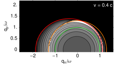
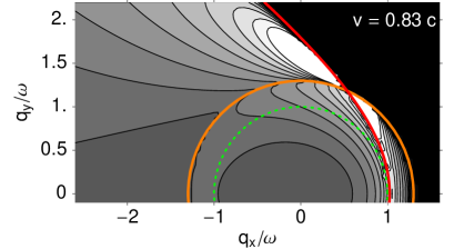
Figure 1: Spectrum of electromagnetic energy per area $U(\omega,{\bf q})$ between two dielectric bodies, one moving at velocity $v$ along the $x$-axis, at a fixed frequency $\omega$. Parameters: zero temperature, refractive index $n=1.3$ (for both bodies in their respective rest frames, frequency-independent for simplicity), distance $a=0.4/\omega\approx 0.064$ free-space wavelengths. The contours give the dimensionless quantity $U(\omega,{\bf q})$ in steps of $0.1$ between $0$ and $1.3$, higher values are clipped (white area), same scale in both panels. Dotted Green circle (radius $q=\omega$): free-space light cone; orange circle (radius $q=n\omega$): propagating photons in the dielectric at rest (‘polariton cone’). Red ellipse (hyperbola): polariton cone in moving dielectric, as seen from the laboratory frame. (left panel) Velocity below Cherenkov threshold $v_{c}=c/n$: the polariton cone is an ellipse. (right panel) $v$ above Cherenkov threshold: the polaritons of the moving dielectric fill two hyperboloids. A non-zero energy spectrum, but with less structure, is found on the other hyperboloid at $q_{x}>q_{x1}\approx 5.9\,\omega$ [Eq.(E.27)].

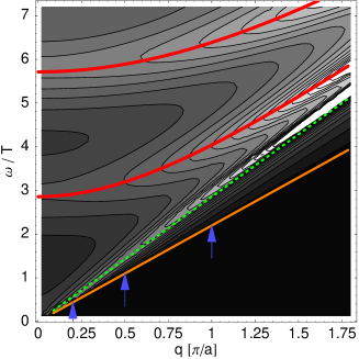
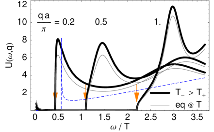
Figure 2: Energy spectrum between a hot dielectric and a cold metallic plate. (left panel) The contours give the dimensionless spectrum $U(\omega,q)$ in steps of $1$ from $0$ to $17$. Red lines: modes in a perfectly reflecting cavity. Dotted green line: light cone $\omega=q$, orange line: polariton cone in the dielectric $\omega=q/n$. The blue arrows mark the cuts shown in the (right panel): energy density vs. frequency $\omega$. Thin lines: two different temperatures (same as left panel), thin gray lines: global equilibrium at the average temperature $T=\frac{1}{2}(T_{+}+T_{-})$, dashed line: free-space spectrum at $T=0$.
Parameters (for a reference temperature $T=300\,{\rm K}$): dielectric at $T_{-}=390\,{\rm K}$ with index $n=1.3$, metal at $T_{+}=210\,{\rm K}$ with impedance $\zeta(\omega)$ such that the skin depth at $\omega=T$ is $\approx 31\,{\rm nm}$. We calculate the impedance from a Drude conductivity with relaxation time $\tau=1.1/T\approx 28\,{\rm fs}$. We have taken a relatively large distance $a=1.1\,\lambda_{T}$ in order to push the cavity resonances (red lines) into the thermal spectral range ($\lambda_{T}=1/T\approx 7.6\,\mu{\rm m}$).

To illustrate the general case, we use Eq.(E.7) and the representation (VI.7) for $\hat{D}^{K}(\Omega;z,z^{\prime})$. In addition, we integrate the energy density over the cavity volume $-a/2<z<a/2$ in order to reduce the number of relevant parameters. The resulting spectrum $U(\omega,{\bf q})$ of the energy per area is dimensionless and plotted in the following as a function of frequency $\omega$ and wave vector ${\bf q}$. We consider for illustration purposes two complementary situations: (a) two dielectric bodies with frequency-independent permittivity (index) $\varepsilon=n^{2}$ at zero temperature $T_{\pm}=0$, the upper one moving at velocity $v$ along the $x$-axis. Situation (b) is taken in mechanical equilibrium ($v=0$) at two different temperatures $T_{+}\neq T_{-}$. One body is metallic, the other one dielectric as before.

Fig.1 illustrates the momentum distribution $U(\omega,{\bf q})$ of the energy spectrum in the ${\bf q}$ plane, at fixed frequency $\omega$. The parameters of the bodies are given in the caption. By inspection of the formulas, we find that the surface sources have a spectral support inside the ‘polariton cone’ where the medium wave vector $q_{z\varepsilon}$ is real [see Eq.(III.5)], i.e., $q\leq n\omega$ (orange circle). If the dielectric is moving, the border of the polariton cone is described by the equation $q_{z\varepsilon}^{\prime}=0$ or explicitly

$$[1-(nv)^{2}]q_{x}^{2}+2(n^{2}-1)v\omega q_{x}+q_{y}^{2}=(n^{2}-v^{2})\omega^{2}$$ (E.26)

For small enough velocity $v$, this describes an ellipse (left panel, red) that intersects the $q_{x}$ axis at

$$q_{x1,2}=\omega\frac{v\pm n}{1\pm nv}$$ (E.27)

Above the Cherenkov threshold, i.e., $v>1/n$, Eq.(E.26) describes two hyperbolas (right panel, red line). It is interesting that the simple setting of a dielectric in fast motion creates a situation quite similar to so-called hyperbolic or indefinite media. These have been studied recently; they show similar dispersion relations in the bulk and are approximately realized in meta-materials with an anisotropic dielectric response Smith_2004 ; Smolyaninov_2010 ; Guo_2012 ; Biehs_2012 .

A setting with two temperatures is illustrated in Fig.2: a hot dielectric facing a cold metal, both at rest. Here, cylindrical symmetry holds and the energy spectrum $U(\omega,q)$ depends only on the modulus $q$ of the parallel wave vector. In the $q\omega$-plane, one identifies the light and polariton cones (dotted green and orange), and the resonances of the planar cavity (red lines). The latter are quite weak because the dielectric plate is a poor reflector. The right panel in Fig.2 shows broad peaks in the energy density at these resonances, as well as sharper features just inside the polariton cone (arrows). The spectrum differs from a global equilibrium situation (thin gray lines). This difference becomes small if $T_{\pm}$ are close, as expected, but also for a highly conducting metal. The energy density is positive everywhere because we did not subtract the vacuum energy density (dotted blue line). The latter eventually dominates at large frequencies.

References

• (1) H. B. G. Casimir, Proc. Kon. Ned. Akad. Wet. 51, 793–95 (1948).
• (2) D. A. R. Dalvit, P. W. Milonni, D. Roberts, and F. da Rosa (eds.), Casimir physics, Lecture Notes in Physics, Vol. 834 (Springer, Berlin Heidelberg, 2011).
• (3) J. Schwinger, J. Math. Phys. 2(3), 407–32 (1961).
• (4) L. V. Keldysh, Sov. Phys. JETP 20(4), 1018–26 (1965), [Zh. Eksp. Teor. Fiz. 47(4), 1515–27 (1964)].
• (5) M. Janowicz, D. Reddig, and M. Holthaus, Phys. Rev. A 68, 043823 (2003).
• (6) Y. Sherkunov, Phys. Rev. A 72, 052703 (2005), 75, 012705 (2007); 79, 032101 (2009).
• (7) V. Mkrtchian, Armen. J. Phys. 1, 229–233 (2009).
• (8) J. W. Negele and H. Orland, Quantum Many-Particle Systems (Westview Press, 1988).
• (9) M. Bordag, D. Robaschik, and E. Wieczorek, Ann. Phys. (N.Y.) 165(1), 192–213 (1985).
• (10) H. Li and M. Kardar, Phys. Rev. Lett. 67(23), 3275–78 (1991).
• (11) H. Li and M. Kardar, Phys. Rev. A 46(10), 6490–6500 (1992).
• (12) T. Emig, A. Hanke, R. Golestanian, and M. Kardar, Phys. Rev. Lett. 87, 260402 (2001).
• (13) T. Emig, A. Hanke, R. Golestanian, and M. Kardar, Phys. Rev. A 67, 022114 (2003).
• (14) T. Emig and R. Büscher, Nucl. Phys. B 696(3), 468–91 (2004).
• (15) M. Born and E. Wolf, Principles of Optics (Pergamon Press, Oxford, 1970).
• (16) M. Soltani, J. Sarabadani, F. Kheirandish, and H. Rabbani, Phys. Rev. A 82, 042512 (2010).
• (17) R. O. Behunin and B. L. Hu, J. Phys. A 43, 012001 (2010).
• (18) R. O. Behunin and B. L. Hu, Phys. Rev. A 82, 022507 (2010).
• (19) A. Kamenev and A. Levchenko, Adv. Phys. 58(3), 197–319 (2009).
• (20) A. Altland and B. Simons, Condensed Matter Field Theory (Cambridge University Press, 2010).
• (21) G. Pieplow, H. R. Haakh, and C. Henkel, Int. J. Mod. Phys. Conf. Ser. 14, 460–66 (2012).
• (22) E. M. Lifshitz and L. P. Pitaevskii, Statistical Physics (Part 2), 2nd edition, Landau and Lifshitz, Course of Theoretical Physics, Vol. 9 (Pergamon, Oxford, 1980).
• (23) W. Eckhardt, Opt. Commun 41(5), 305–09 (1982).
• (24) E. M. Lifshitz and L. P. Pitaevskii, Physical Kinetics (Butterworth-Heinemann, Oxford, 1991).
• (25) C. Henkel, K. Joulain, J. P. Mulet, and J. J. Greffet, J. Opt. A: Pure Appl. Opt. 4(5), S109–14 (2002).
• (26) V. G. Polevoi, Sov. Phys. JETP 71(6), 1119–24 (1990).
• (27) A. A. Kyasov and G. V. Dedkov, Nucl. Instr. Meth. Phys. Res. B 195(3-4), 247–58 (2002).
• (28) G. V. Dedkov and A. A. Kyasov, Tech. Phys. Lett. 28(12), 997–1000 (2002).
• (29) G. Pieplow and C. Henkel, New J. Phys. 15, 023027 (2013).
• (30) V. L. Ginzburg, Phys. Uspekhi 39(10), 973–82 (1996).
• (31) T. G. Philbin and U. Leonhardt, New J. Phys. 11, 033035 (2009).
• (32) J. M. Jauch and K. M. Watson, Phys. Rev. 74(8), 950–57 (1948).
• (33) G. V. Dedkov and A. A. Kyasov, Surf. Sci. 604(5-6), 562–67 (2010).
• (34) J. B. Pendry, New J. Phys. 12, 033028 (2010).
• (35) G. Barton, J. Phys.: Condens. Matter 23, 355004 (2011).
• (36) V. B. Beresteckii, E. M. Lifshitz, and L. P. Pitaevskii, Quantum Electrodynamics (Pergamon Press, Oxford, 1982).
• (37) M. F. Maghrebi, R. Golestanian, and M. Kardar, Quantum Cherenkov Radiation and Non-contact Friction, arXiv:1304.4909, 2013.
• (38) L. D. Landau, E. M. Lifshitz, and L. P. Pitaevskii, Electrodynamics of continuous media, 2nd edition (Pergamon, Oxford, 1984).
• (39) I. A. Dorofeyev and E. A. Vinogradov, Phys. Rep. 504(2-4), 75–143 (2011).
• (40) S. M. Rytov, Theory of Electrical Fluctuations and Thermal Radiation (Publishing House, Academy of Sciences USSR, Moscow, 1953).
• (41) V. Sopova and L. H. Ford, Phys. Rev. D 66(4), 045026 (2002).
• (42) D. R. Smith, P. Kolinko, and D. Schurig, J. Opt. Soc. Am. B 21(5), 1032–43 (2004).
• (43) I. I. Smolyaninov and E. E. Narimanov, Phys. Rev. Lett. 105, 067402 (2010).
• (44) Y. Guo, C. L. Cortes, S. Molesky, and Z. Jacob, Appl. Phys. Lett. 101(13), 131106 (2012).
• (45) S. A. Biehs, M. Tschikin, and P. Ben-Abdallah, Phys. Rev. Lett. 109(10), 104301 (2012).